the Creative Commons Attribution 4.0 License.
the Creative Commons Attribution 4.0 License.
 | 31 Jan 2024
The 4D reconstruction of dynamic geological evolution processes for renowned geological features
Zhibin Liu
Xulei Wang
Shanjun Liu
Yunqiang Li
The three-dimensional (3D) visualization of geological structures and the dynamic simulation of geological evolutionary processes are helpful when studying the formation of renowned geological features. However, most of the existing 3D modeling software is based on raster models, which are unable to generate smooth geological boundaries. This work proposes a 3D temporally dynamic (i.e., four-dimensional (4D)) modeling method using parametric functions and vector data structures, which can dynamically build geological evolutionary vector models of well-known geological features. First, we extract the typical features of different kinds of geological formations and represent them using different parameters. Next, we select appropriate parametric functions to simulate these geological formations according to the characteristics of the individual structures. Then, we design and develop 4D vector modeling software to simulate the geological evolution of these features. Finally, we simulate an area with complex geological structures and select six real-world geological features, such as the Piqiang Fault in China and the Eye of the Sahara in the Sahara Desert, as case studies. The modeling results show that a regional geological evolutionary model that contains smooth boundaries can be established within minutes using this method. This work will support studies into the formation of renowned geological features in terms of providing visualizations and will make the representation of geological processes more intuitive in 3D.
- Article
(9641 KB) - Full-text XML
- BibTeX
- EndNote


Geological relics are features on the surface of the earth that manifested at some point during the earth's geological history. The analysis of regional geological evolutionary processes is central to the study of how geological relics formed. Regional geological evolution refers to the process of continuous change and transformation of a geological body due to the action of certain regional forces (be they external, internal, or man-made). Eventually, these forces alter the composition and structure of the local stratigraphic units and can change the surface morphology. Understanding the evolutionary processes that impact geological formations is critical to the study of geological evolution, because not only do these processes control the formation and evolution of fractures but also determine the spreading and superposition of other geological structures. The analysis of geological evolutionary processes also plays a crucial role in determining structural morphology, assessing bioaccumulation, and assessing coalbed gas and the abundance of mineral resources (Favre et al., 2015; Li et al., 2021; Rahbek et al., 2019; Zhai and Santosh, 2013; Zhou et al., 2022). Therefore, studying the geological and structural evolution of a region and simulating it can help people better understand how the geology of the region developed.
The traditional method of studying geological evolutionary processes is to analyze the data directly and then visualize the results obtained from the analysis in the form of geological cross-sections and profiles (Bozzano et al., 2008; van Hinsbergen et al., 2020). Some researchers also use static 3D models for these visualizations. A common method of interpretation involves using the survey data to develop a geological model for a specific moment in time and then extracting cross-sections along arbitrary directions within the 3D model (Abdullah et al., 2022; Adelu et al., 2019), which makes the interpretation process much easier. Essentially, the evolutionary process is still represented within the cross-section. However, subsurface geological phenomena are 3D by nature, and two-dimensional (2D) profiles cannot clearly express the complete evolution of the subsurface. These specialized 2D depictions of the evolutionary processes are not sufficient visual representations of the geologist's ideas and knowledge. They are only convenient for discussing and disseminating knowledge among peers and experts (Lidal et al., 2012). These products remain inaccessible to general audiences and make communicating ideas challenging. This is a problem since geologists prefer to be able to communicate their results in a way that can be understood by nonexperts and decision makers alike.
Therefore, the numerical simulations are also applied to geological evolutionary studies. This involves conducting simulation experiments for each phase of structural movement and adjusting the simulation parameters as the experiments progress. Finally, the actual evolutionary processes operating within the modeled domain are obtained (Chen et al., 2010; Wu et al., 2022). There are also scholars who use existing software, such as some by Adobe, to manually draw and animate the geological evolution process to facilitate communication (Geology – an Introduction, 2012). However, these methods present their own challenges. They are not automatically generated and are time-consuming to generate, and because of a lack of generality between individual models, the researcher may be required to start over for different geological regions, which leads to highly repetitive workflows.
Natali et al. (2012) proposed a method for synthesizing 3D models from 2D sketches. Based on this, Lidal et al. (2013) proposed a sketch-based approach to reconstruct geological evolutionary processes, which allows for the model process to be visualized and for the reasoning behind it to be more clearly conveyed. This approach can quickly construct a 3D geological evolutionary model from hand sketches. However, the final model obtained by this method only adds a depth to the 2D image and the structure along the depth direction cannot be simulated. Jessell and Valenta (1966) and Jessell et al. (2022) proposed an integrated orthorectification technique for simulating the geophysical response of 3D structures and geological bodies that have undergone multiple stages of deformation. This method can simulate the deformation history of a region by including a series of historical events and the model can then obtain the corresponding geological data. Cockett et al. (2016) created a learning tool, Visible Geology, capable of exploring the evolutionary processes of different geological bodies in one-dimensional (1D), 2D, and 3D space. However, these techniques all have some drawbacks and the method used to simulate geological structures is too simple. For example, the generated folds can only run through the whole model, the intrusive rocks are represented as a simple layer of vertical strata, and the models are all raster models, which cannot smoothly depict geological boundaries (Zhu et al., 2022). Therefore, there has been a lack of a 4D vector modeling method for the simulation of geological evolutionary processes. This method includes more modules available for feature construction and can quickly reconstruct dynamic geological evolutionary processes, which can then be communicated to a general audience.
Geological evolutionary processes are generally inferred by geological experts based on scattered data and their own knowledge. Therefore, it is difficult to clearly represent a complete evolutionary process with only 2D pencil and paper drawings. It will not only take a lot of time to model each process, but the geological data for each process cannot be obtained to support this endeavor. Here we propose a method to quickly construct a model that simulates geological evolutionary processes according to the need for the process to be visually expressed. First, this model is generalized and parameterized for various complex geological formations that may have occurred during geological evolution. Then, different parameter functions are used to simulate the different kinds of geological formations. Second, each kind of geological structure is modularized, and a tetrahedron field is used to organize the whole model so that it can easily incorporate a geological structure module to the current model. This method can model geological evolution quickly and dynamically based on our software. Finally, the key operations of changing geological morphology are stored for each step of the geological timeline, which can easily replicate the entire evolution process. Additionally, each operation in the history timeline is exported for subsequent reproduction and modification. Using this technique, geologists can quickly construct a simplified history of geotectonic motion for a region based on the geological information considered (such as the evolution of the regional geology).
In this study, we modularized five geological structures, including tilt, fold, fault, simple unconformity, and intrusive rocks, which can be superimposed in any order. This article is structured as follows: Sect. 2 presents the rationale for the generalization of each geological formation, Sect. 3 describes the simulation methods used for each formation, Sect. 4 performs a typical case simulation, Sect. 5 discusses recommendations for future research, and Sect. 6 presents the conclusion.
First, this study generalizes some basic geological formations, and different kinds of geological structures are parameterized according to the basic elements of geological formations. This enables the model to differentiate geological structures and to separate them into different modules, thus ensuring that a diversity of geological structures is expressed within the model so as to better simulate the diverse forms of geological structures found in nature.
2.1 Stratigraphic data
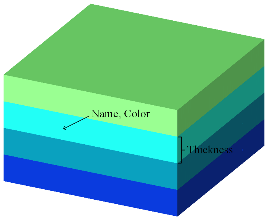
A stratum is a layer or group of rock layers that has some uniform characteristics and properties and is clearly distinguishable from the units above and below. In this study, we simulate the simplest sedimentary stratum by reducing sedimentary strata that may have some variable thickness to a uniform thickness. Therefore, for the simplified stratigraphy, a stratum can be described by the following three parameters (Fig. 1): name, which denotes the name of the stratum; color, which indicates the color used to represent the stratum and is also used to represent a certain stratum characteristic or certain group of stratum characteristics; and thickness, which refers to the thickness of this homogeneous stratum.
2.2 Geological structure data
2.2.1 Folds
In nature, fold refers to a stratum that has been subjected to strong forces and structural stress that results in continuous wavy and undulating morphology. The portion of the fold that is bent upwards is called an anticline, and a syncline is where the fold is bent downwards. In general, folds are rarely formed by only one force and are often the result of at least horizontal or inclined compressional forces and gravity. The formation of folds in nature may involve more complex forces, resulting in a variety of fold forms. Therefore, based on geological terminology, this work selectively simplifies and parameterizes fold structures by using fold elements that describe the shape and occurrence of folds. The basic components of folds (Fig. 2a) include the following:
- –
The core of the fold, which indicates the rock layer at the center of the fold.
- –
The limb, which refers to the area where the sides of the fold are relatively straight.
- –
The hinge zone, which refers to the curved portion where the two wings of the fold join. Here the morphology can be categorized as circular, sharp angled, box shaped, or knee shaped. Additionally, folds can be described, for example, as arch-like folds, chevron folds, box folds, fan folds, or flexures.
- –
The hinge, which refers to the location of maximum bending on the fold surface. Hinges are mostly straight lines but may also be curved or folded lines, and its yield is horizontal, inclined, or upright, which represents the variability of the fold along the direction of its extension.
- –
The axial plane is where the hinge of the adjacent folded surface is connected to form a hypothetical marker surface, which is mostly flat and straight but can also be curved. The intersection of the axial plane with the ground or any other plane is called the axial trace.
- –
The inflection point is the dividing point between the dorsal and diagonal vectors along the continuous fold waveform, i.e., the point where the curvature of the fold is zero.
- –
The apex line (also called the ridge line) and trough line refer to the lines that connect the highest points of the same anticline and the lowest points of the same syncline, respectively.
We first simplify folds into periodic oscillatory global folds according to the geological characteristics of folds. For the hinge zone, only the more common rounded, pointed prismatic, and boxed shapes are considered in this study. This study simplifies the hinge as a straight, horizontally oriented line. Depending on the subsequent tilt of the geological structure, the orientation can be changed to inclined or vertical. This work simplifies the axial plane to a flat surface and similarly makes the apex and trough lines straight. Therefore, the fold becomes a periodic fold according to the simplification method, with each cycle having the same morphology, and for a single cycle, it is described by the following five parameters (Fig. 2b): height, which is the vertical distance from the hinge to the inflection point; position, which is the position of the entire fold in the horizontal direction and is represented by the distance of the inflection point from the origin; cycle length, which is the distance covered by a single cycle in a fold; angle, which is the inclination of the axis surface and is characterized by the angle between the axis surface and the horizontal surface; and shape, which is the shape of the hinge zone and indicates the transition between sharp-angled and box-shaped folds, and the midpoint represents the circular fold.
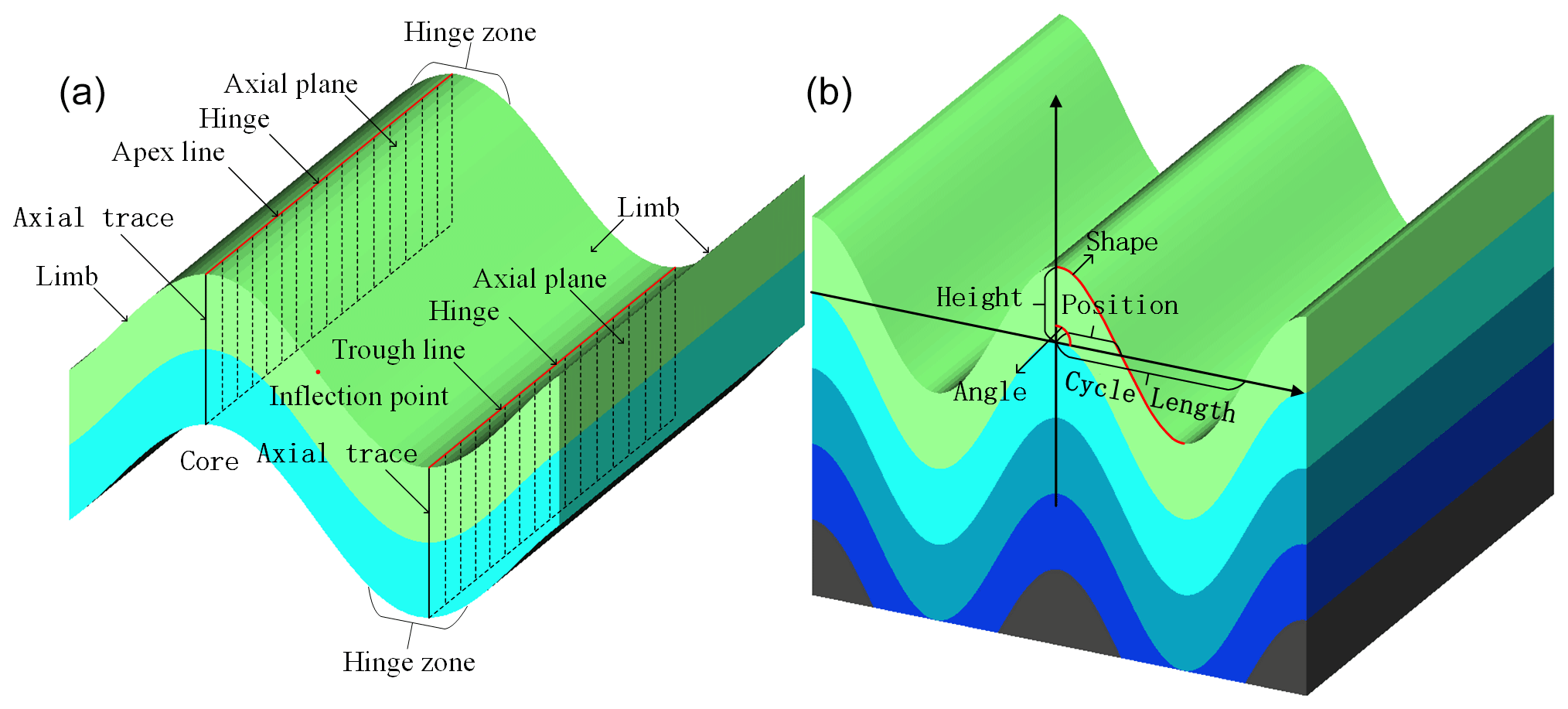
Figure 2Fold structure generalization schematic: (a) fold elements and (b) fold parameterization principle.
2.2.2 Partial folds
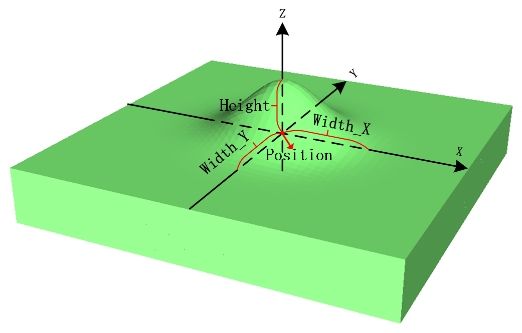
In practice, folds do not necessarily run through the entire study area, and thus it is not possible to consider only the global fold. It is also necessary to implement the ability to add a local fold at any position in the study area. In this work, we simplify the partial folds and consider them only as raised or recessed for a distance around the selected position. Therefore, with reference to the definition of the fold parameters, the partial folds are described by the following four parameters based on the geological terminology and simplification process (Fig. 3): position, which refers to the coordinates of the center of the fold (X, Y) and is used to indicate the position of the added fold; height, which is the vertical distance from the topmost part of this local fold to the position point; width_X, i.e., the X direction fold degree parameter, which is the influence range of the partial fold in the X direction and is used to indicate the maximum distance of this partial fold along the x axis; and width_Y, which is the Y direction fold degree parameter, defined similarly to width_X.
2.2.3 Tilts
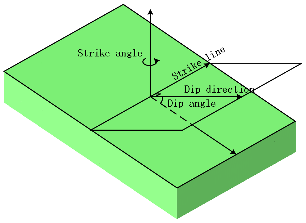
The tilt structure is a rock formation that has a certain angle between the rock plane and the horizontal plane after the structure changes. If the tilt direction and dip angle of a set of tilted rock formations in a certain area are largely the same, it is called a single-slope structure, which is the simplest form of tilt. There are three main types of tilted structure rock formations: fold structures with only a single wing, a disk of fault structures, or faults caused by uneven uplift or downwards movement in the region. Determining the orientation of tilted rock formations is the basis for studying tilted geological formations. Tilt is determined by measuring the direction of extension of the rock plane in 3D space and the angle with a geodetic level (horizontal plane). Tilt measurements consist of three elements of orientation – strike, dip, and dip angle (Fig. 4) – described as follows:
- –
The straight line where the rock layer intersects the horizontal plane is called the strike line, and the direction indicated by the strike line is the direction of the rock layer, which indicates the extension direction of the rock layer in space.
- –
Dip refers to the line on the rock formation that is perpendicular to the strike line and extends downwards along the slope (i.e., the true tilt line). The projection of the true tilt line in the horizontal plane is the strike line and the direction indicated by the strike line is the tendency of the rock formation.
- –
The dip angle is the angle between the true inclination line and the true tilt line.
This study simplifies and parameterizes the tilted structure based on the geological characteristics of the tilted structure and the three elements of orientation. First, the tilted structures are reduced to the simplest single-slope structures. Since it is known that the tendency line and the strike line are perpendicular to each other based on the character of the orientation, the following two parameters (Fig. 4) can be used to describe the tilted structures: strike angle, which is the angle between the strike line, and due north represents the orientation of the strike element; and dip angle, which is the angle between the inclination line and the tilt line, which also indicates the angle between the tilted rock formation. The horizontal plane represents orientation of the dip angle.
2.2.4 Faults
A fault is a geological formation in which a rock layer or a rock body is fractured by force and the rock masses on both sides are significantly displaced relative to each other along the ruptured surface. Faults are common features in the earth's crust, and they vary in size and scale, from large faults extending hundreds to thousands of meters along the strike to small faults of only a few tens of centimeters. Faults are some of the most important structures related to the movement of the earth's crust. Geometric elements of faults are the basis of fault geometry studies and include the fault surface, fault line, fault disk, and fault distance (Fig. 5a). The fault plane constitutes the ruptured surface of the fault, that is, the surface formed by significant relative sliding of rock bodies along both sides of the fault. The fault plane is generally composed of a series of rupture surfaces or secondary fault zones and is, therefore, also called the fault zone or fracture surface. Similarly, we can describe the spatial location of the fault surface in terms of the three orientation elements. The fault line refers to the intersecting line between the fault surface and the ground, and the direction of the fault line is the strike of the fault. The fault wall is the location of relative displacement on both sides of the fault and is divided into the hanging wall and lower foot wall. Distance of displacement is the distance between the two fault walls and the location of relative sliding along the fault plane. Faults can be divided into three categories, compressional faults, tensional faults, and torsional faults. Additionally, faults can be classified according to their mechanical properties and the relative motion of the fault disk; these are normal faults, reversed faults, parallel faults, and hinge faults.
We simplify the fault surface into a plane and express its location with three elements of orientation according to the fault elements and fault classification. We simplify the relative motion of both disks of the fault as translational motion considering the simplicity of parameter expression. Although all faults in nature have some rotation, the angle is generally not large. Therefore, only normal faults, reversed faults, parallel faults, and their combination of fault types are considered in this work (Fig. 6). Thus, the fault can be described by the following parameters (Fig. 5b):
- –
Orientation parameters, such as the tilted structure, are used to describe the orientation of the fault plane, namely, the two variables strike angle and dip angle.
- –
Position, the location parameter, is used to describe the center location of the fault plane in the study area.
- –
Moving angle, the relative sliding angle, is used to describe the moving direction of the hanging wall relative to the foot wall.
- –
Moving distance, i.e., slip distance, is used to describe the distance of fault elements such as the distance between two walls where relative slip occurs.
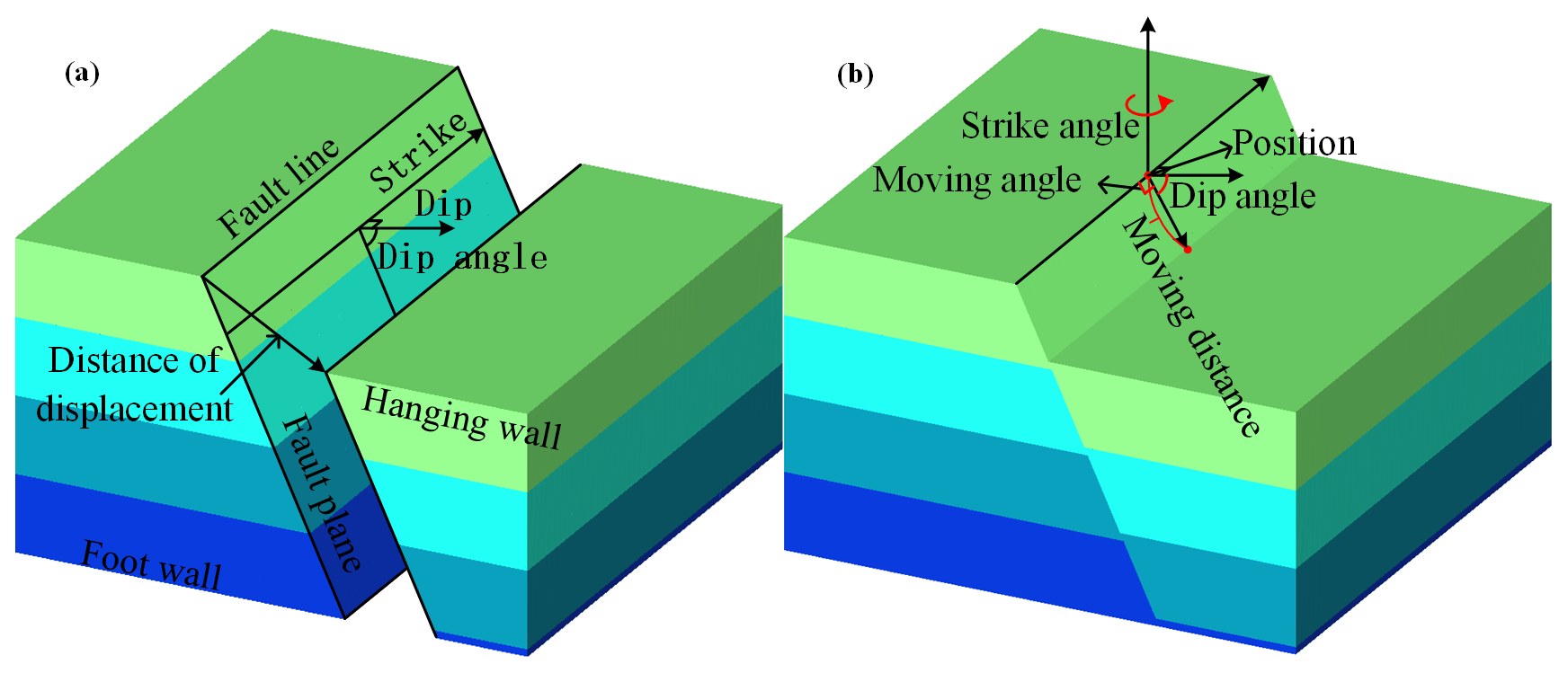
Figure 5Fault structure generalization schematic: (a) fault elements and (b) fault parameterization principle.
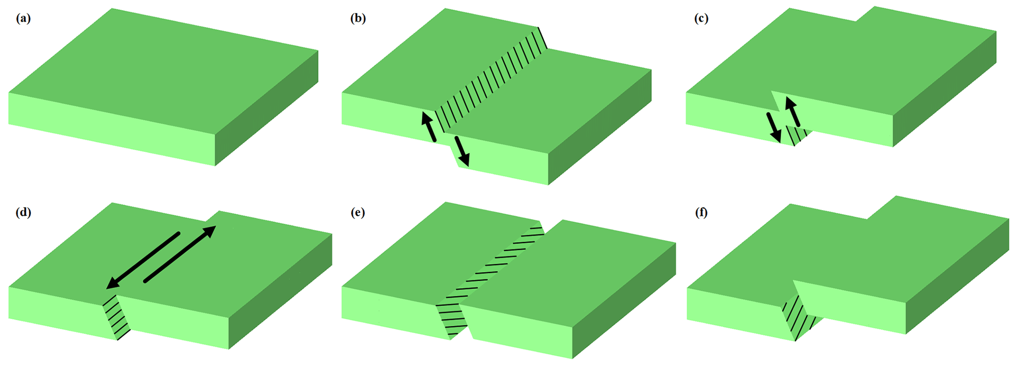
Figure 6Fault combination type: (a) normal rock formation, (b) normal fault, (c) reversed fault, (d) parallel fault, (e) parallel normal fault, and (f) parallel reversed fault.
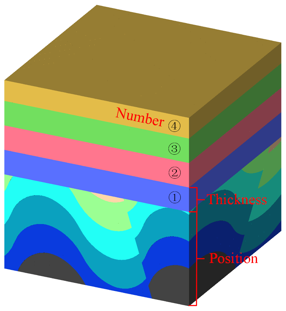
2.2.5 Unconformities
Unconformities describe stratigraphic relationships between two sets of adjacent strata of different ages above and below where depositional interruptions or stratigraphic deficiencies have occurred. An unconformity is generally classified as being either an angular unconformity or a pseudo-conformity (also known as disconformity). An angular unconformity refers to two sets of strata that are in contact at an angle, and a pseudo-conformity refers to two sets of strata that are in roughly parallel contact. The interface between two sets of strata in contact is called the erosion surface (also called the unconformity surface).
We first simplify the contact surface, i.e., the unconformity plane, to a horizontal plane according to the characteristics of the unconformity, and then the set of strata above the contact surface are simplified according to the simple sedimentary stratigraphy presented in this paper (Sect. 2.1). Therefore, the following parameters are used to describe the unconformity structure (Fig. 7): position, i.e., the height position parameter, which refers to the position of the horizontal plane within the model area; number, i.e., the number of strata, which refers to the number of layers in a set of sedimentary strata above the contact; and thickness, which refers to the thickness of each layer of a set of sedimentary strata above the contact.
2.2.6 Intrusive rocks
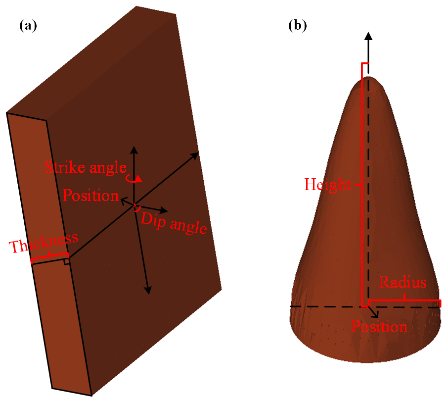
Intrusive rocks refer to the rocks formed when the pressure of the overlying rock layer decreases, and the magma invades the rock layer or fissures in the crust from below and then gradually cools and solidifies within the earth. Intrusive rocks can be divided into stocks, apophyses, dikes, sheets, and batholiths according to different occurrences. In this study, only stock and dikes are considered. Since batholiths and apophyses rarely appear, these two categories are not considered at this time. Simulating the other two categories according to their morphology reveals that the stocks are unconformable intrusions that extend downwards in a trunk-like pattern on a larger scale, while dikes, also known as “rock walls”, are a more commonly distributed intrusive vein. Dikes are similar to slab-like rocks filled with fissures that cut across the rock layer and intersects the laminae obliquely, which is a kind of intrusive unconformity. Therefore, the shape of the dikes is slab-like and the stock is columnar.
We simplify the dikes into flat plates and the strains into synapses according to the shape of the veins and strains. Therefore, the following parameters can be used to describe each of these two intrusive rock forms: dikes (Fig. 8a) can be described based on their orientation parameters (i.e., strike angle and dip angle), position, and thickness. The strike and dip angles refer to the tilted structure of the dike and are used to describe the dike posture, while the position parameter describes the central location of the dike and thickness describes the dike thickness. Stocks (Fig. 8b) can be described in terms of their position, radius, and height. The position parameter refers to the planar location of the centroid of the stock. The radius parameter refers to the radius of the bottom end of the stock and is used to describe the extent of the stock, and the height parameter describes the maximum elevation to which the rock has intruded.
3.1 Construct strata
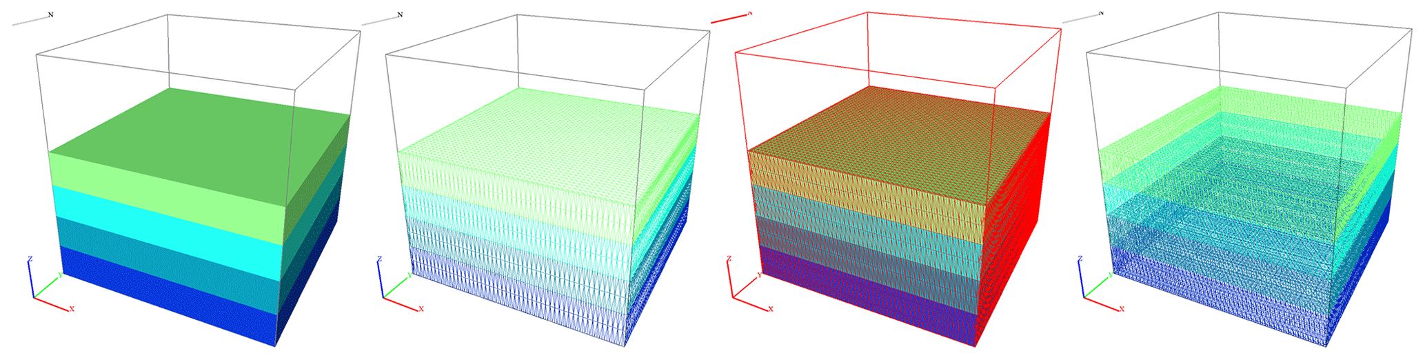
The strata are the basis of the whole evolutionary process, and all methodological modules of geological formations are carried out on the strata. Therefore, for the numerical representation of the geological body, a suitable data model is needed. Here we use a tetrahedral model (Fig. 8) to construct the stratigraphic model as opposed to a hexahedral model (Bagley et al., 2016) or other model type. There are several advantages of organizing within tetrahedral forms compared with other models. First, a tetrahedral raster field can contain more triangular surfaces with the same accuracy and can represent the geological model more precisely. Second, calculating the intersection of a face with a tetrahedron is much easier. Third, the tetrahedron can be divided iteratively. The space of a tetrahedron can be continually divided into two parts, which can still be represented by the tetrahedron. Fourth, the tetrahedral raster field provides a better structural basis for model analysis and model operators such as arbitrary planar sectioning, excavation in different ways, and volume statistics (Guo et al., 2021). The above advantages provide the possibility of repeatedly adding geological formations, ensuring that regardless of the operation being carried out, the whole model is still represented by tetrahedron.
3.2 Folds
3.2.1 Global folds
In the 3D geological model, we simulate the folding action by introducing a vertical shear model. The shear action is defined by the combination of displacement field and rotational field . Considering the different forms of folds (mainly arch-like folds, chevron folds, and box folds are considered), the displacement field is defined as a complex superposition of three functions. The arch-like fold is defined as a cosine function (Eq. 1), the chevron fold is defined as a jagged segmented periodic function (Eq. 2), and the box fold is defined as a segmented combined higher-order periodic function (Eq. 3):
where A, ω, and φ are chosen within a certain range and these three parameters represent the height of the fold, the degree of the fold, and the position of the fold. Then, f1, f2, and f3 are combined by a shape parameter δ in the range to obtain the shearing fields where −1 represents the chevron folds, 0 represents the arch-like folds, 1 represents the box shape, and the shapes are combined using Eq. (4):
Then, the simulation of the fold axial plane angle α is realized by using the combination of the plane function (Eq. 5) and the rotation fields RY and S0. First, S0 and f4 are combined to obtain the final displacement field S1 according to Eq. (6), then the rotation of the axial plane angle is realized using the rotate field RY (Eq. 7):
where RY(θY) is a 3D rotation matrix rotated about the Y axis and θY is the rotation angle around the y axis. Using this rotation field to rotate the final displacement field by the −α angle around the y axis, i.e., , the axis plane is successfully tilted by the α angle. This displacement field is only used to create the shape of the fold along the X direction.
However, the above methods can only simulate folds along the X direction and cannot simulate folds in any other direction. Therefore, this study further makes use of the rotation equation around the z axis (Eq. 8) to enable the folds to be added in any direction.
The rotation field is a 3D rotation matrix rotating around the z axis, and θz is the angle around the Z direction, chosen within a certain range. Here we construct the following rotation field (Eq. 9) using the rotation matrix so that the axes of the rotation field translate to the center point of the model . The rotational field is used in several subsequent constructions and will not be frequently repeated:
Using the combination of the shear displacement field and the rotation field in Eq. (10), we can add a fold structure to the original geological model (Fig. 10a, in Eq. (10) to obtain a new folded geological model (Fig. 10e–g; in Eq. 10):
Figure 10b–d show the fold preview morphology of the fold model (Fig. 10e, f, g). We can clearly see the pattern of the fold to be added. By choosing the displacement field parameters A, ω, φ, and α, and the rotation field parameter θ, we can add any overall fold configuration with different bending structures that we need to the model. In Fig. 10, panels b and e, c and f, and d and g are the fold surface preview and fold simulation results of arch-like folds, chevron folds, and box folds, respectively.
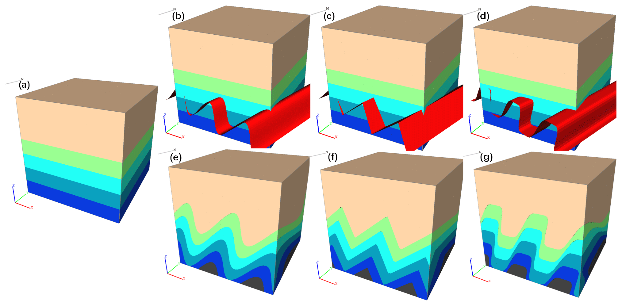
Figure 10The fold structure effect: (a) original geological model, (b) arch-like fold preview, (c) chevron fold preview, (d) box fold preview, (e) arch-like fold result model, (f) chevron fold result model, and (g) box fold result model.
3.2.2 Partial folds
We have implemented the fold module, but the fold module runs through the overall model. In fact, folds generally do not occur evenly in the whole study area according to the different geological characteristics, but there will be partial folds. Thus, the global folding module alone is not sufficient for the evolution of most geological situations. Therefore, in this study, the Gaussian function Eq. (11) is used to propose the local translation field to realize the partial fold module (Wu et al., 2020) according to the morphology of the partial fold definition:
where A, σx, and σy are selected within a certain range as parameters to control the form of the partial fold, A controls the pleat height, and σx and σy control the degree of pleat intensity in the X and Y directions; the larger the fold is, the more intense. (Xo,Yo) is the center point of the fold, and the default is the center point of the model but can also be replaced by selected points. Therefore, the translation field realized by this method can add local folds along the X direction or Y direction.
Similarly, the rotational field is further utilized to enable the addition of local folds in any direction. The rotational field is detailed in Eq. (9) and will not be repeated here.
Combining the above displacement field and rotation field , we obtain Eq. (12). Therefore, by using Eq. (12), we can add a fold structure to the original geological space (Fig. 11a; in Eq. 12) to obtain a new folded geological space (Fig. 11c; in Eq. 12):
Figure 11b shows a preview of the partial fold. By the above method, we can add different morphological structures to the model at any position we need for local fold construction. With the above methods, we can add partial folds of different morphologies and structures to the model at any position.
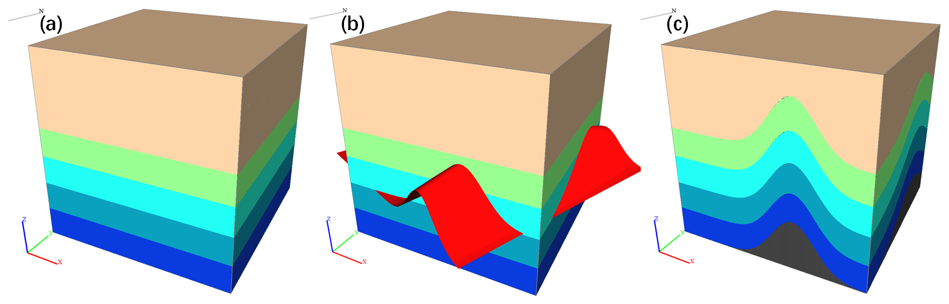
Figure 11Adding the partial fold: (a) original geological model, (b) partial fold preview, and (c) partial fold result model.
3.3 Tilts
The stratigraphic tilt structure is realized by rotating the 3D structural model, and the rotation angle, i.e., the tilt angle of the model, is determined by two angles or rotation around one z axis (rotation matrix in Eq. 8) and one y axis (rotation matrix in Eq. 13):
The overall 3D model is then rotated around the center of the model to achieve the desired angle by the two rotation fields (Eqs. 9 and 14). The principle is similar to that of the partial fold rotation field, which is not repeated here:
By rotating the two rotation fields and along the axis of the model midpoint (Eq. 15), a new tilted 3D geological structure (Fig. 12c; in Eq. 15) can be obtained by adding a tilted structure from any angle to the original 3D geological structure (Fig. 12a; in Eq. 15):
Figure 12b shows a preview of the surface of the tilt angle. By combining the above method with the tetrahedral raster field, the addition of the tilted geological structure can be realized while ensuring that the topological relationship remains unchanged.
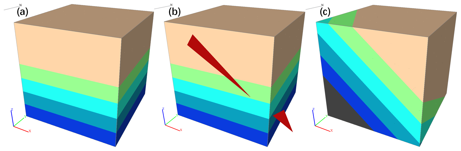
Figure 12Adding the tilt effect: (a) original geological model, (b) tilt preview, and (c) tilt result model.
3.4 Faults
Faults are an important type of geological structure. Here we use the moving tetrahedron method (Guo et al., 2021) to divide the stratigraphy within the tetrahedron grid field according to the specified fault plane. Then, the two parts obtained after the division are interwoven to simulate the fault. In order to make the selection of parameters more intuitive, we use a plane (Eq. 16) parallel to the y axis and a rotational field (Eq. 9) rotating around the z axis to determine the appropriate fault plane:
where a is the slope of the plane, determined by the dip of the fault plane, and b is the location parameter of the fault plane, which can change the spatial location of the fault plane. The rotation field can rotate the fault surface to the corresponding angle according to the strike and dip of the fault plane; therefore, the plane can express the fault plane at any angle and the fault structure can move in any direction. Then, adding another rotational field on the fault plane can change the displacement direction of fault.
Additionally, a point p(Xo,YoZo) on the fault plane and a vector parallel to the X–O–Z plane and the fault plane (the vector orientation varies with the rotation angle of the selected rotation field on the fault plane and defaults to a downwards orientation) and a vector normal to the fault plane at that point are obtained before the parameters of the fault plane are selected. The point p and the two normal vectors vary accordingly with the selected fault surface parameters so that the point p is always on the surface, m is always along the fault surface, and n is always normal to the fault surface.
Furthermore, before selecting each parameter of the fault plane, we define point on the fault plane, a vector across point p and parallel to the X–O–Z plane and the fault plane, and a normal vector of the fault plane across point p. The point p and the two vectors vary accordingly with the selected fault plane parameters, ensuring that the point p is always on the surface, m is always along the fault surface and n is always the normal vector of the fault plane.
After the parameters of the fault surface are determined, the point p on the fault surface and the two vectors are also determined. Then, point p and normal vector n are brought into Eq. (17) to obtain the point normal expression:
After obtaining the equations of the fault surface, we used the moving tetrahedron method to divide the 3D geological structure organized by the tetrahedral grid field into two parts according to the fault surface; part 1 is above the fault surface and part 2 is below. Then, the whole of part is moved along the direction of vector m by a distance δ (entered when selecting each parameter of the fault plane) to obtain (Eq. 18). The direction of m is downwards by default, which in this work indicates a normal fault. The −m vector is used if a reversed fault is selected, though this can also be modified according to the rotation angle of the rotational field located on the plane to achieve different directions and thus simulate a walking slip fault. Finally, the two parts are combined by stratigraphic correlation to obtain the final fault model:
Using the above method, we can obtain a new geological structure (Fig. 13c) after simulating the occurrence of normal faults (Fig. 13b1), reverse faults (Fig. 13b2), or parallel faults (Fig. 13b3) at any location of the original geological structure (Fig. 13a), where Fig. 13b is a preview of the surface when selecting the location of the fault plane.
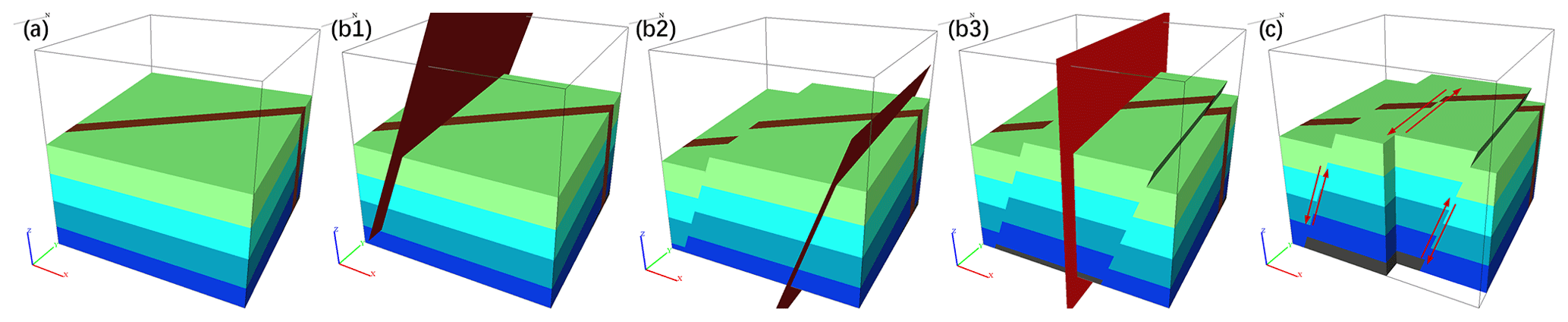
Figure 13Adding the fault: (a) original geological model, (b1) normal fault preview, (b2) reverse fault preview, (b3) parallel fault preview, and (c) fault result model.
3.5 Unconformities
Stratigraphic unconformities are also an important and frequently occurring structural phenomenon, and it is necessary to understand the underlying causes before simulating them. The development of unconformity surfaces starts with the deposition of older strata, followed by crustal movement and the exposure of older strata to surface erosion, and finally the deposition of newer strata according to the principle of unconformity structure parameterization above. Simply put, the surface is eroded first and then material is subsequently deposited.
Therefore, following this feature, we use a similar method to add a series of new sedimentary strata to the original geomorphic body. However, the model is cut at the location of the additions using a method that simulates the fault structure before adding the unconformity, and only the lower part is retained to simulate denudation. The cutting operation simply divides the original geological body at the location where stratigraphy will be added using a plane parallel to X–O–Y. (The detailed procedure is described in the simulated faults section and will not be described here.)
By using this cut-then-add method, we can simulate a simple unconformity within the original geological structure (Fig. 14a) to obtain a new 3D geological structure (Fig. 14c). Figure 14b shows a preview of the added unconformity, and we can preview and modify the location, number of strata, and thickness of the strata to be added.
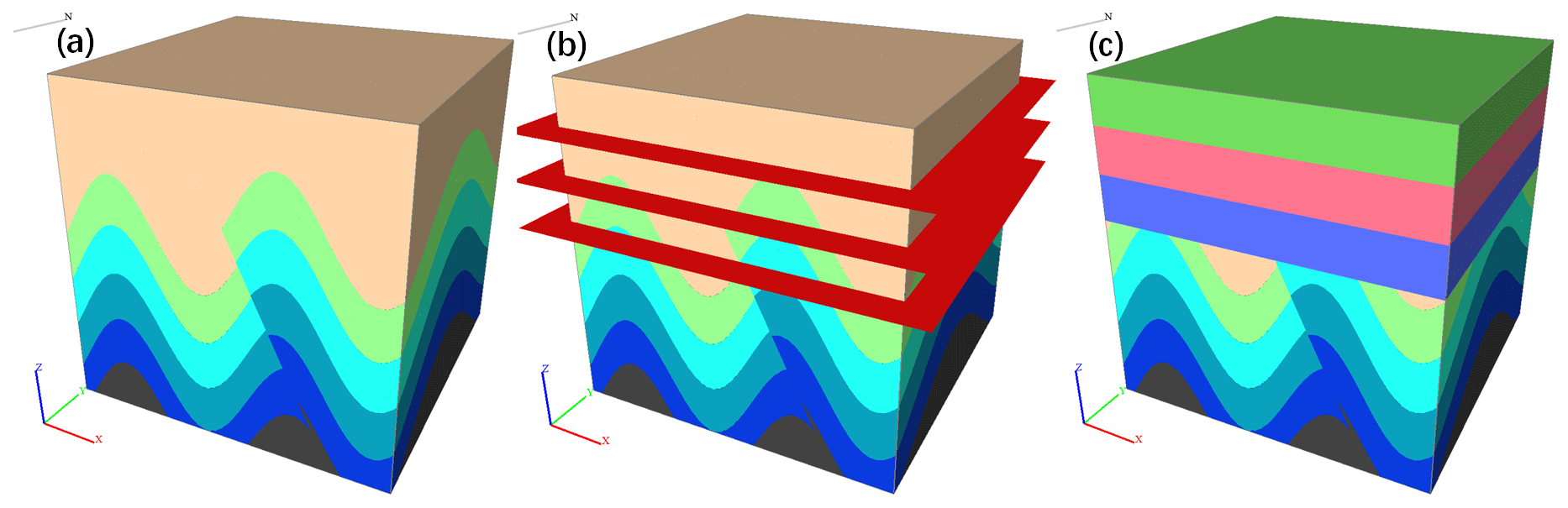
Figure 14Adding the unconformity: (a) original geological model, (b) unconformity preview, and (c) final unconformity model result.
3.6 Intrusive rocks
We use two parallel planes (Eq. 19) and (Eq. 20) with δ intervals to represent the dike and use one Gaussian plane (Eq. 21) to represent the stock according to the shape characteristics of the dike and stock discussed above. The two parallel planes are used to cut the structure to obtain a model body of a certain thickness, and then the geological properties of this model body are changed to an intrusive dike. The Gaussian surface is used to simulate the stock thereby dividing the model using the Gaussian surface to obtain a columnar body and similarly changing the geological properties of this geological body to reflect the intrusive stock:
By using the above two simple functions to cut and then change the properties, we can successfully add the intrusive dike or stock to the original geological structure (Fig. 15a) to obtain a new geological body (Fig. 15c and e, where (c) is a dike and (e) is a stock). Figure 15b and d show the preview of intrusive rocks to be added, which can be added according to the change in parameters such as location and morphology of the intrusive rocks.
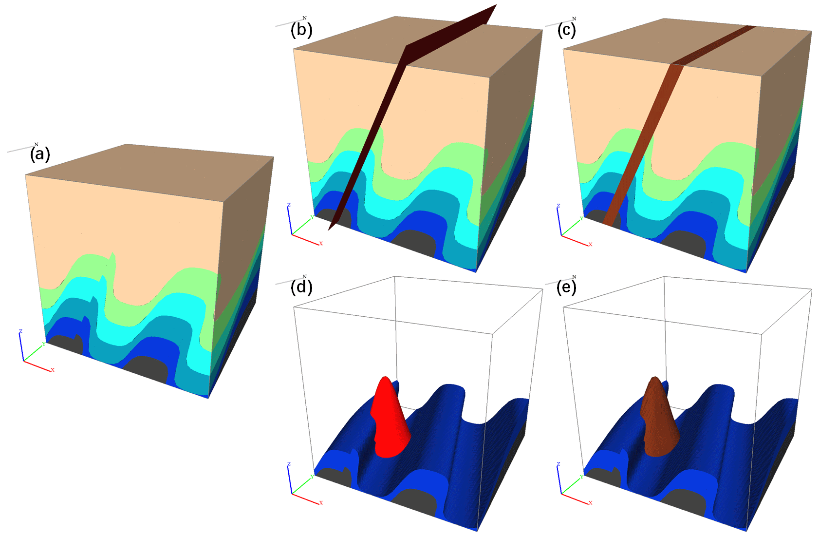
Figure 15Adding the intrusive rock (dike and stock): (a) original geological model, (b) intrusive dike preview, (c) intrusive stock preview, (d) intrusive dike result model, and (e) intrusive stock result model.
We developed a 4D geological structure evolution vector modeling program using the Qt 5.9.1 (2023) framework (https://www.qt.io/, last access: 5 October 2023) based on the simulation method presented in this work. Then, we conducted the case studies below using this software. The geological models obtained from the simulations in this section were constructed using a laptop computer (AMD Ryzen9 5900HX 3.3 GHz, 16 GB of RAM, and an NVIDIA GeForce RTX 3060). Case 1 simulates the construction of a complex geological structure based on a series of geological events. Case 2 selects six typical geological features in the world and simulates their evolutionary processes. First, we infer the historical evolutionary process of typical complex geological formations and then simulate the evolutionary process by using the method developed by this study. Finally, each geological event and corresponding geological model can be clearly viewed according to the historical timeline provided by the model to reveal the 4D reconstruction of geological features. Thus, the formation process of complex geological structures in the region can be intuitively and clearly understood. We can also save the final modeled processes for review, modification, and editing.
4.1 Case 1: simulation of complex regional geological and structural evolutionary processes
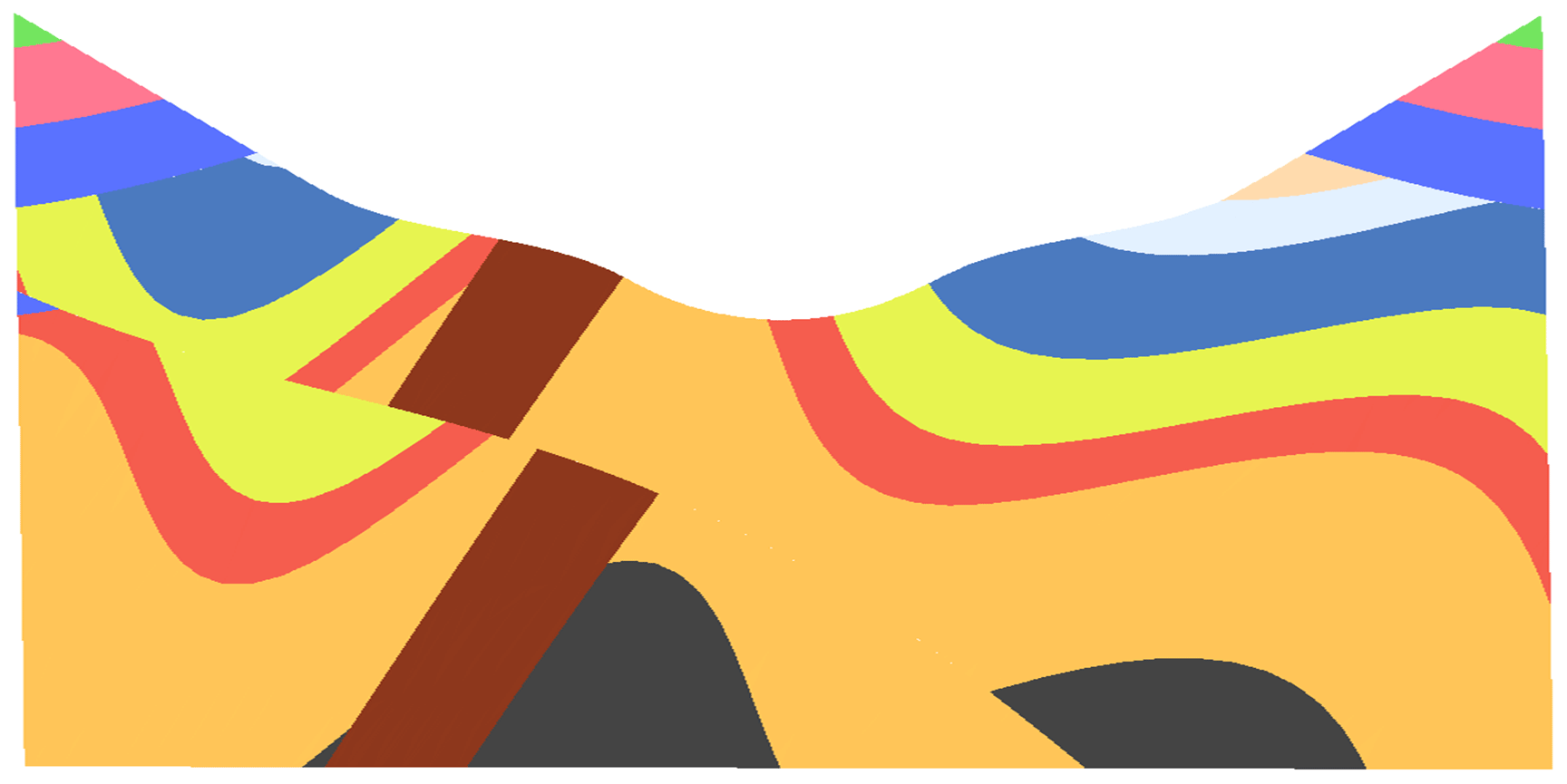
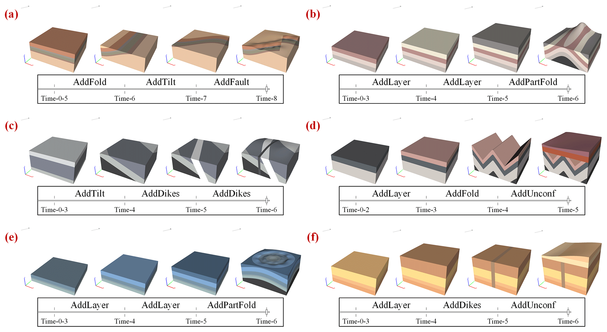
If we want to study the evolutionary process of features in complex regions with many different types of geological structures, we generally deconstruct the existing geology from a geological profile (Fig. 16), which requires not only strong professional knowledge but also a certain degree of spatial approximation. It is also difficult to extrapolate feature evolution moving forwards through time according to the information within the geological section.
In contrast, using the forwards simulation software presented in this paper, it is easy to construct historical geological events according to feature evolution. Combining the temporal dimension and the process of regional structure development, the model clearly and visually shows the forms of interaction between new geological events and pre-existing geology and structures. For example, the existing regional geological history was developed from a series of stratigraphic depositional events, folding, tilting, unconformities, diking, faulting, and stocking. The results of a series of events simulated using the geological evolution modeling program presented in this paper are shown in Fig. 17. The software presented here also has different built-in terrain functions, including flat land, hills, ridges, valleys, and cliffs, and we choose the valley terrain in this case (Fig. 17i).
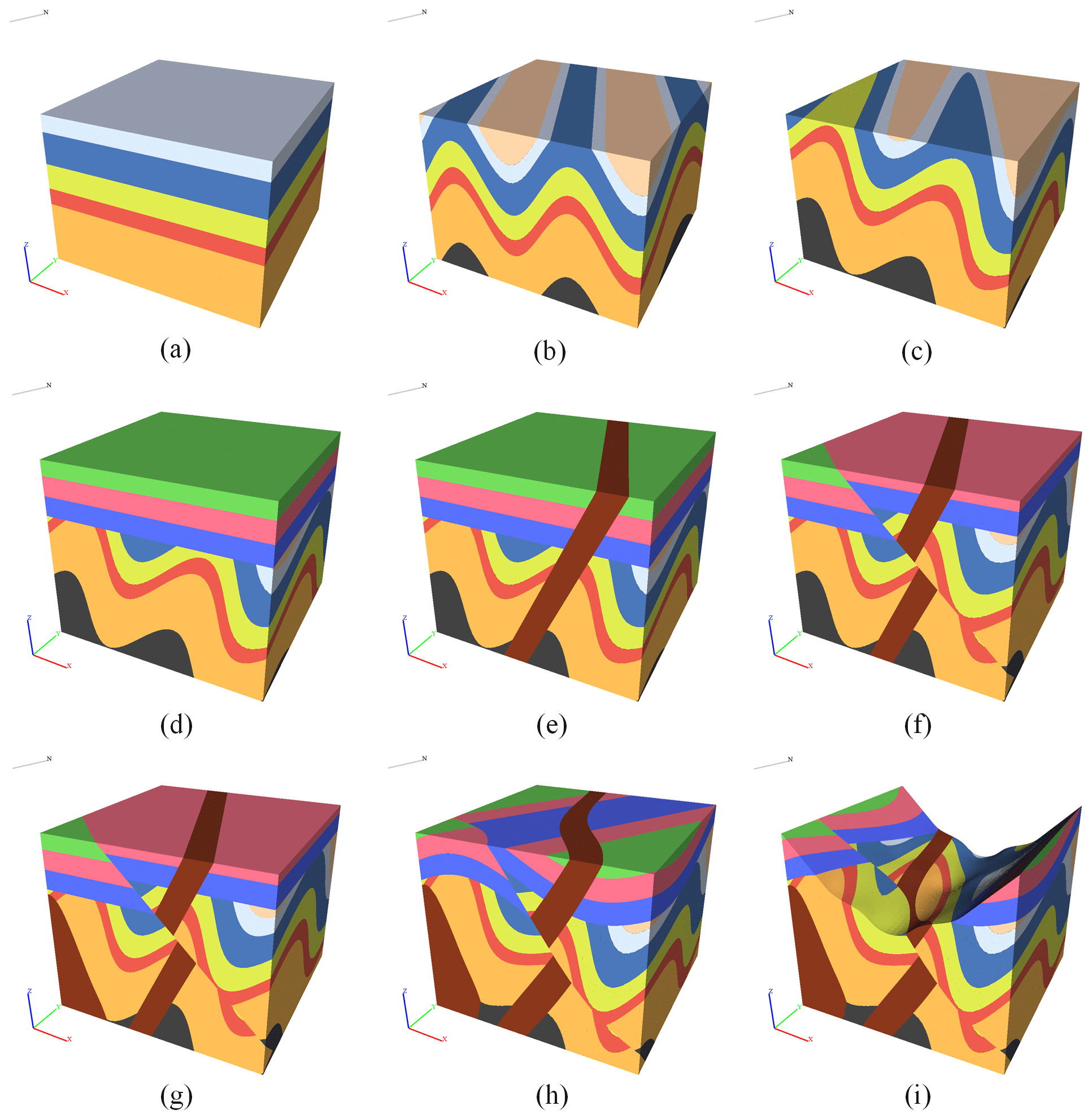
Figure 17Complex regional geological and structural evolutionary process simulation results: (a) strata, (b) fold, (c) tilt, (d) unconformity, (e) dike, (f) fault, (g) stock, (h) fold, and (i) valley terrain.
Based on the simulation results, it can be concluded that this method can sufficiently simulate the evolutionary process of complex geological structures. It is easy to add various geological events using the methods outlined in this article due to the modularity of the model process. The user can add arbitrary construction events based on the inferred historical evolution and check the correctness of the inferred evolution based on the results of the combined events. This can only be achieved in a simulation that progresses forwards through time, because we can clearly see the effect of each process in the subsequent geological formations that overprint on the previous geological formations. For example, in Fig. 18a and b, the folded and tilted geological structure is folded in front and tilted at the back. The effect is different if the tilt is in front and the fold is behind (e.g., see Fig. 18c and d).
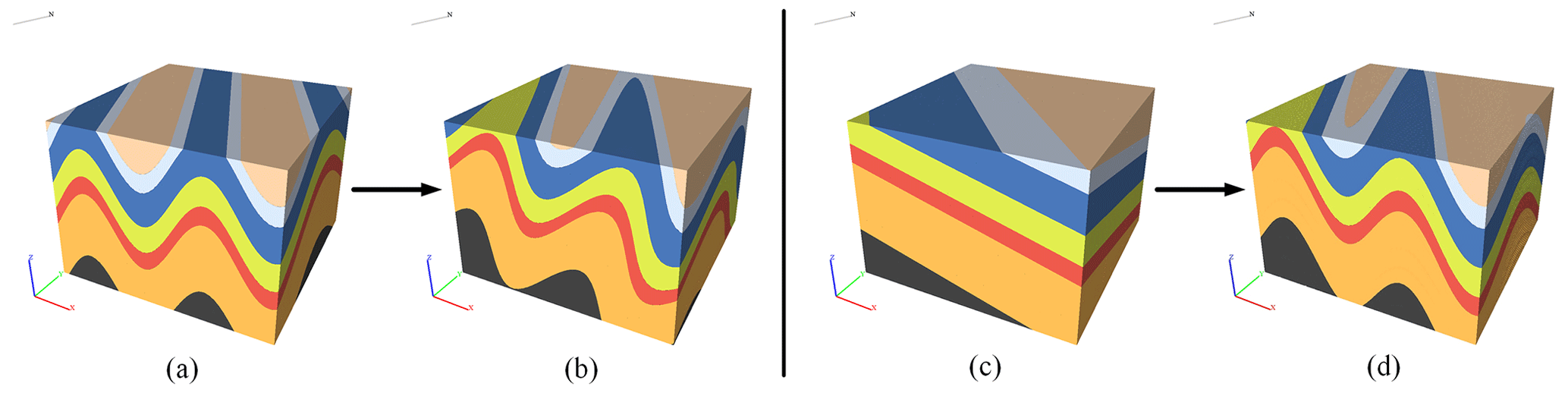
Figure 18Different sequences of geological structural development and the influence on the results. Panels (a, b) show that the tilted structure occurs after the folded structure and (c, d) show that the tilted structure occurs in front of the folded structure.
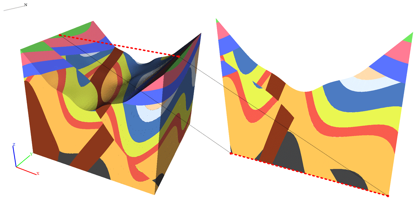
The software also provides the ability to view the history of the model in series via the model timeline and freely creates sections after generating the final model. Thus, it is possible to view the historical evolution of the model dynamically (Fig. 19) by bringing up the model timeline. The timeline records each geological event that affected the model and the time it occurred. (User inputs, such as time node shown in Table 1, can be changed.) It can help people more intuitively understand the correlation between 2D sections and 3D geological event processes when combined with the function of generating corresponding sections by freely selecting two points on the final model.
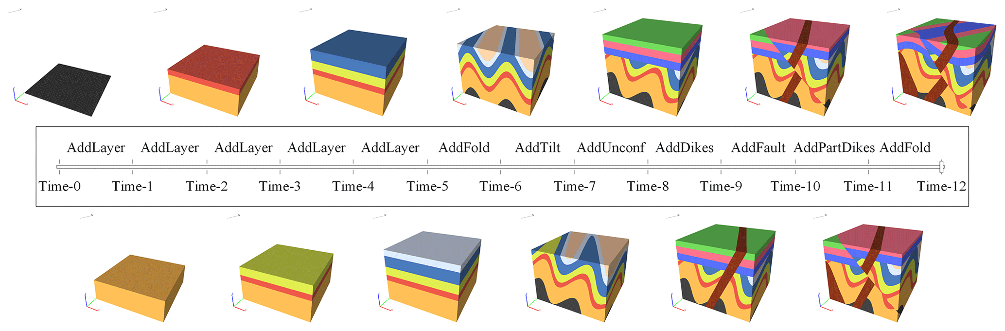
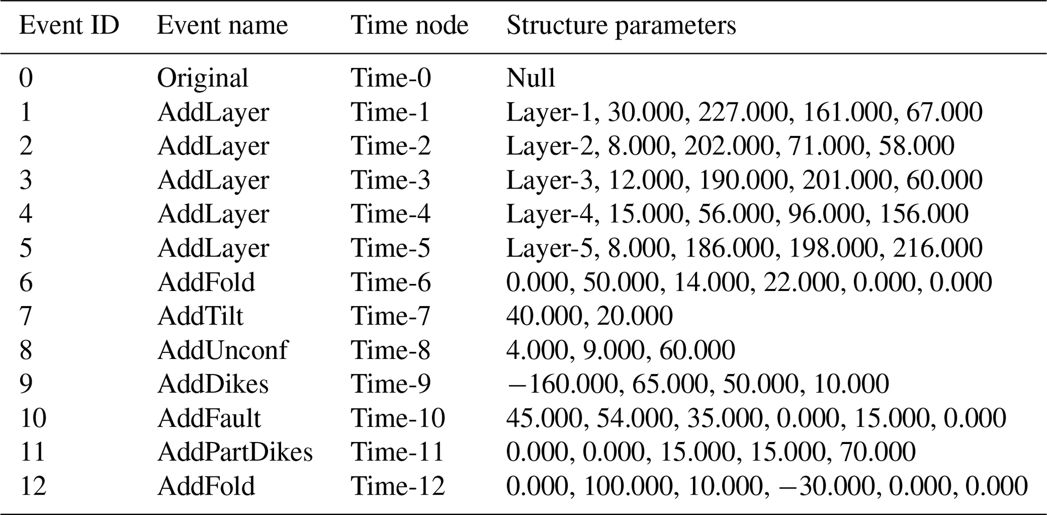
Finally, the model's geological event process also supports saving and importing, allowing the user to save the entire historical evolution of the final model (i.e., each geological event affecting the model) as a historical process table file (Table 1), and the software supports reopening the file to easily reproduce the evolutionary process. This means that if only the data for a geological event are available, we can generate simulation results by directly inputting these deterministic results into the file. Furthermore, we can fine tune the saved evolutionary process file to quickly modify the parameters of a particular geological event, and we can also automatically generate table files via scripting to enable rapid generation of a great quantity of simulated geological models.
4.2 Case 2: simulating the evolutionary process of typical geological features
The simulation software presented in this work was used to simulate typical geological features from six geological sites from around the world (Fig. 20):
- a.
The Piqiang Fault, which is located in the Tarim Basin of Xinjiang in China. This is a northwest-trending strike-slip fault in which the reddish, greenish, and brownish bands are continental Devonian sandstones, Silurian deeper marine sediments, and Cambro-Ordovician limestones, respectively.
- b.
Sheep Mountain in Wyoming, USA, which is a partially folded structure.
- c.
Kosterhavet National Park on Yttre Ursholmen Island in the Koster Islands in Sweden contains multiple stages of pyrogenic intrusion. An igneous intrusion is first cut by a pegmatite dike, which in turn is cut by a dolerite dike.
- d.
Located in Telheiro Beach in Portugal is a typical angular geological unconformity positioned between the schists and metagreywackes of the “Brejeira Formation” from the Upper Carboniferous and new red sandstones of the “Grés de Silves Formation” from the Triassic.
- e.
The Richat Structure, also named the “Eye of the Sahara”, is a prominent circular geological feature in the Sahara's Adrar Plateau. Initially, it was thought to be caused by a meteorite impact, but it lacked the impact signature of a subsidence ring and evidence of stratigraphic overturning; thus, the possibility of a meteorite impact was negated. However, other scholars thought it was caused by a volcanic eruption, but this theory was also rejected because of the lack of volcanic rock or a dome of igneous rocks. Currently, academics generally agree that it is a highly symmetrical and deeply eroded geological dome (Matton and Jébrak, 2014).
- f.
Located in Makhtesh Ramon in the Negev Desert in Israel is a feature formed by a dike and unconformities. Additionally, the area is recognized as a heritage site by the Council for Conservation of Heritage Sites in Israel.
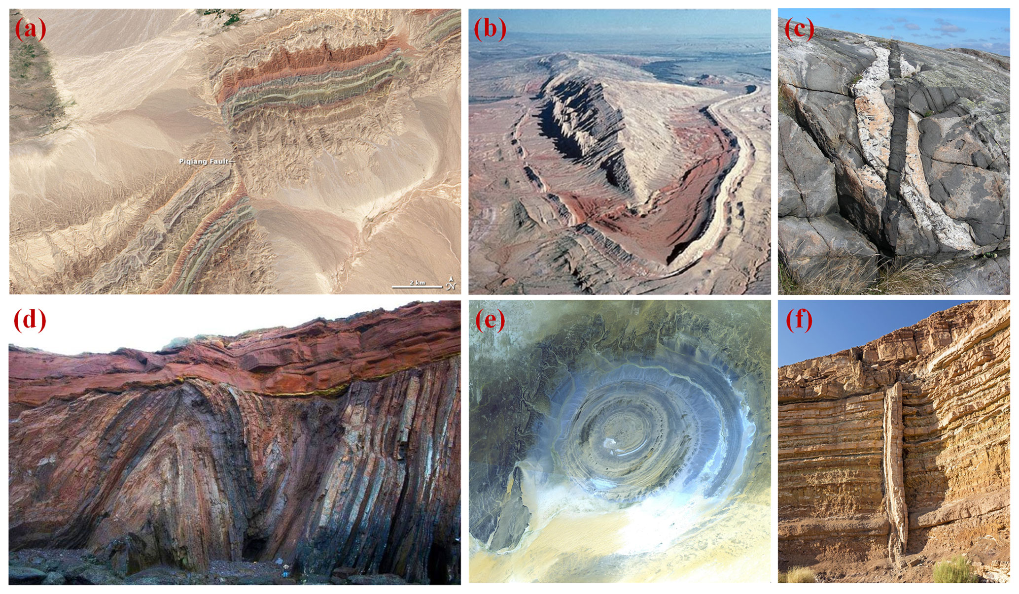
Figure 20Geological sites and typical features. Figure sources: (a) Piqiang Fault, China (https://commons.wikimedia.org/wiki/File:Piqiang_Fault,_China_detail.jpg?uselang=en, last access: 3 January 2023); (b) Sheep Mountain, United States (https://www.geowyo.com/ancient-river-channel--sheep-mountain.html, last access: 3 January 2023); (c) Multiple Igneous Intrusion Phases, Sweden (https://commons.wikimedia.org/wiki/File:Multiple_Igneous_Intrusion_Phases_Kosterhavet_Sweden.jpg, last access: 3 January 2023); (d) Angular Unconformity, Portugal (https://www.geologyin.com/2015/01/amazing-angular-unconformity.html, last access: 3 January 2023); (e) Richat Structure, Ouadane, Mauritania (https://commons.wikimedia.org/wiki/File:ASTER_Richat.jpg?uselang=en, last access: 3 January 2023); and (f) Geological dike, Makhtesh Ramon, Israel (https://commons.wikimedia.org/wiki/File:ISR-2016-Makhtesh_Ramon-Geological_dike.jpg, last access: 3 January 2023).
First, we must analyze and obtain their geological evolution to model the structural evolution of the aforementioned geological sites (Fig. 20). The geological sites selected in this paper all have typical structural forms; therefore, we mainly analyze the formation process of these typical structures prior to the simulation:
- a.
The Piqiang Fault is on the northwest side of the Bachu Fault zone and is connected to the Bachu Uplift in the south. Because of the uplift in the south, the stratigraphy of the area shown tends to dip to the north of the strike-slip fault (Turner et al., 2011).
- b.
This is a partial fold, but with erosion of relatively weak parts on both sides. The harder sandstone in the interior is cut into a ridge, while the weaker shale around it is eroded (Bellahsen and Fiore, 2005).
- c.
According to the description given by the source, this is an igneous intrusion cut by a pegmatite dike, which in turn is cut by a dolerite dike, and stratigraphic tilting occurred before the intrusion began.
- d.
This is a typical angular unconformity that began when the underlying strata were formed, which were then folded by crustal movement before finally being eroded and redeposited to form the overlying new strata.
- e.
This feature is a symmetrical and deeply eroded geodome. The circular distribution of ridges and valleys is interpreted to have been formed by differential erosion of alternating hard and soft rock layers uplifted as a dome by underlying Cretaceous alkaline igneous complexes (Matton et al., 2005).
- f.
This feature was formed by the superposition of a dike and an unconformity; the dike occurred first, according to the image, and then the unconformity followed.
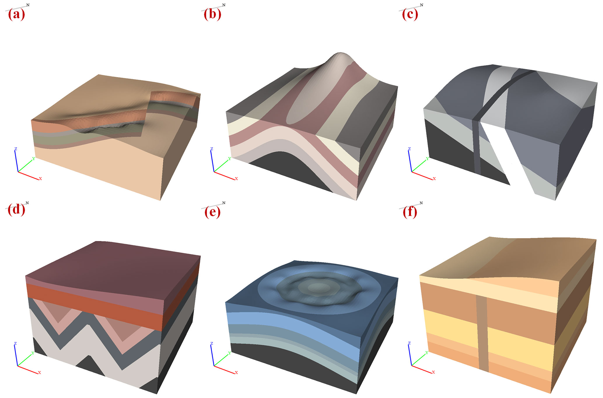
The structural evolutionary processes of the above geological features were simulated using the simulation software presented in this paper, and the results of the simulation are shown in Fig. 21. The results show that the structural evolutionary sequence of common geological features can be correctly and quickly simulated using the geological evolution simulation software. If only the time of model generation is considered, the modeling times of (a)–(f) are 22, 17, 29, 16, 14, and 15 s, with an average of only 18 s. Through the timelines provided by the software (the timelines for the geological features are shown in Fig. 22), the formation process and principle of typical geological structures in geological features can be dynamically observed and the 4D reconstruction of the evolution process of geological features can be achieved. This enables users to more clearly and intuitively understand the morphology and modes of action of local structures.
This paper proposes a method to simplify and express various types of basic geological formations and establishes regional geological evolutionary process simulation and visualization software based on this method, which can assist geologists in explaining the evolutionary processes of geological features. The fact that geologists find it very difficult to visualize these processes in 3D is a very common problem; therefore, these processes are still often expressed in 2D section form for geological interpretation. In practical applications, subsurface geological phenomena are by nature 3D, and it is difficult to clearly express the evolution of geological formations in 3D space using 2D sections. Our method makes it possible to represent the evolutionary geotectonic processes in a 3D environment. With two case studies, we also show that the method presented in this paper can support the rapid simulation of regional geotectonic evolutionary processes in 3D space.
Our proposed method supports the simulation of geological structures in any direction and angle within the X, Y, and Z coordinate frame and can generate vector models with smooth boundaries as compared with other methods capable of visualizing geotectonic evolutionary processes in a 3D environment. Our method summarizes and simplifies each geological structure and incorporates it into a corresponding module, which greatly facilitates the ability of the end user to simulate the structure. Additionally, the method in this paper utilizes different parameter functions to express various geological formations, and the parameter functions are directly applied to the stratigraphy when adding formations. Therefore, it is more convenient to extend and enrich the individual structures by introducing new parameter functions or modifying the existing ones.
We use a tetrahedral grid to arrange strata and structures, and then the vector model is constructed. Therefore, it is possible to extract geological data that cannot be extracted by a raster model, such as geological boundary data. We also provide the free cutting function, which can easily obtain the geological section in any direction along the simulation model (Fig. 23). The software also preserves the interface of each geological structure so that we can generate a great quantity of simulated geological models quickly by writing scripts, and together with the geological simulation data generated, we can automatically generate a great quantity of geological models, along with their corresponding geological data, which can then be used as a training set for deep learning applications.
Our method certainly has some limitations. For example, in this study we simplified individual stratum to a uniform thickness, and although the width and thickness of a stratum should vary, for the sake of simplicity, this paper simplifies the geological strata to have uniform thicknesses. However, this simplification is only applicable when the strata within a region do not undergo erosion and maintain a consistent thickness. Thus, this simplification poses challenges in simulating strata erosion. Similarly, this paper simplifies fault planes as planar surfaces, which limits the ability to simulate curved fault surfaces. Additionally, when considering intrusive rocks, the method used in this study focuses on common occurrences while neglecting the batholiths and apophyses. Therefore, there are limitations in simulating intrusive rocks using the method. Although this method provides many parameters that can add variety to the geological elements, the final product is still far more regular that would be observed in reality. Therefore, the simulation model presented here is not as precise as the model built from actual data. However, this model depicts the evolutionary process that is not reflected in the model developed from actual data. Our subsequent research may be to add more types of elements and further enrich the model to add more possibilities. In future research, it is recommended to consider using appropriate parameter functions to represent geological strata and fault planes, allowing for the nonuniform thickness of strata and simulation of curved fault surfaces. This would overcome the limitations of the current approach and provide more accurate representations of geological formations. Additionally, for different forms of intrusive rocks, modularization using suitable parameter functions can be implemented to improve the applicability of simulating intrusive rocks. This method would enhance the representation of intrusive rock formations and capture the complexities associated with their formation processes.
We parameterized and modularized various geological structures and developed a 4D vector modeling program, which can quickly simulate the evolution of geological structures. We then conducted experiments from two perspectives. First, we simulated the evolution of complex regional geological formations and actual well-known geological features. The results showed that software developed by this study can be used to quickly model the evolution of complex geological structures and simulate the evolution of actual geological features. Finally, the 4D spatial and temporal evolution of regional geological formations was realized. This model can also dynamically present the regional geological evolutionary processes and reveal the interactions between structures over time via the timeline feature of the program. The system presented in this paper was developed around the idea of using several representative parameters to express various geological structures and encapsulate those structures within different modules. Therefore, it is more convenient to add subsequent structures and provide additional detail to a single structure.
The source code of the 4D geological structure evolution vector modeling is available at https://doi.org/10.5281/zenodo.7498592 (Liu and Guo, 2023).
The model data and terrain data of the cases in this paper are available at https://doi.org/10.5281/zenodo.7498592 (Liu and Guo, 2023).
The video of the program built in this paper is available at https://doi.org/10.5281/zenodo.7498592 (Liu and Guo, 2023).
JG and ZL conceived the study. JG provided funding support and ideas. ZL and XW were responsible for the research method and program development. XW and YL helped to improve the modeling method and software. LW and SL helped to improve the manuscript. All authors read and approved the paper.
The contact author has declared that none of the authors has any competing interests.
Publisher's note: Copernicus Publications remains neutral with regard to jurisdictional claims made in the text, published maps, institutional affiliations, or any other geographical representation in this paper. While Copernicus Publications makes every effort to include appropriate place names, the final responsibility lies with the authors.
The authors would like to thank the reviewers for their valuable suggestions that increased the quality of this paper.
This research has been supported by the National Natural Science Foundation of China (grant no. 42172327), the State Key Laboratory of Disaster Prevention & Mitigation of Explosion & Impact (grant no. LGD-SKL-202209), and the Fundamental Research Funds for the Central Universities (grant no. N2201022).
This paper was edited by Mauro Cacace and reviewed by Mauro Cacace and one anonymous referee.
Abdullah, E. A., Abdelmaksoud, A., and Hassan, M. A.: Application of 3D Static Modelling in Reservoir Characterization: A Case Study from the Qishn Formation in Sharyoof Oil Field, Masila Basin, Yemen, Acta Geol. Sin.-Engl., 96, 348–368, https://doi.org/10.1111/1755-6724.14766, 2022.
Adelu, A. O., Aderemi, A. A., Akanji, A. O., Sanuade, O. A., Kaka, S. I., Afolabi, O., Olugbemiga, S., and Oke, R.: Application of 3D static modeling for optimal reservoir characterization, J. Afr. Earth Sci., 152, 184–196, https://doi.org/10.1016/j.jafrearsci.2019.02.014, 2019.
Bagley, B., Sastry, S. P., and Whitaker, R. T.: A Marching-Tetrahedra Algorithm for Feature-Preserving Meshing of Piecewise-Smooth Implicit Surfaces, Procedia Engeer., 163, 162–174, https://doi.org/10.1016/j.proeng.2016.11.042, 2016.
Bellahsen, N. and Fiore, P. E.: The Growth of Sheep Mountain Anticline: Comparison of Field Data and Numerical Modes, Stanford Digital Repository, http://purl.stanford.edu/yv876np7540 (last access: 18 January 2024), 2005.
Bozzano, F., Bretschneider, A., and Martino, S.: Stress–strain history from the geological evolution of the Orvieto and Radicofani cliff slopes (Italy), Landslides, 5, 351–366, https://doi.org/10.1007/s10346-008-0127-2, 2008.
Chen, L., Tang, D. B., Liu, X. B., Oliveira, M., and Liu, C. Q.: Evolution of the ring-like vortices and spike structure in transitional boundary layers, Sci. China Phys. Mech., 53, 514–520, https://doi.org/10.1007/s11433-010-0129-7, 2010.
Cockett, R., Moran, T., and Pidlisecky, A.: Visible Geology: Creative Online Tools for Teaching, Learning, and Communicating Geologic Concepts, American Association of Petroleum Geologists, https://doi.org/10.1306/13561985M1113671, 2016.
Favre, A., Packert, M., Pauls, S. U., Jahnig, S. C., Uhl, D., Michalak, I., and Muellner-Riehl, A. N.: The role of the uplift of the Qinghai-Tibetan Plateau for the evolution of Tibetan biotas, Biol. Rev. Camb. Philos. Soc., 90, 236–253, https://doi.org/10.1111/brv.12107, 2015.
Geology – an Introduction: E-learning module about geology, http://folk.uib.no/nglhe/Emodules/GeoIntroMod.swf (last access: November 2012), 2012.
Guo, J. T., Wang, X. L., Wang, J. M., Dai, X. W., Wu, L. X., Li, C. L., Li, F. D., Liu, S. J., and Jessell, M. W.: Three-dimensional geological modeling and spatial analysis from geotechnical borehole data using an implicit surface and marching tetrahedra algorithm, Eng. Geol., 284, 106047, https://doi.org/10.1016/j.enggeo.2021.106047, 2021.
Jessell, M., Guo, J., Li, Y., Lindsay, M., Scalzo, R., Giraud, J., Pirot, G., Cripps, E., and Ogarko, V.: Into the Noddyverse: a massive data store of 3D geological models for machine learning and inversion applications, Earth Syst. Sci. Data, 14, 381–392, https://doi.org/10.5194/essd-14-381-2022, 2022.
Jessell, M. W. and Valenta, R. K.: Structural geophysics: Integrated structural and geophysical modelling, in: Structural Geology and Personal Computers, edited by: De Paor, D. G., Computer Methods in the Geosciences, Pergamon, 303–324, https://doi.org/10.1016/S1874-561X(96)80027-7, 1996.
Li, J. Z., Tao, X. W., Bai, B., Huang, S. P., Jiang, Q. C., Zhao, Z. Y., Chen, Y. Y., Ma, D. B., Zhang, L. P., Li, N. X., and Song, W.: Geological conditions, reservoir evolution and favorable exploration directions of marine ultra-deep oil and gas in China, Petrol. Explor. Dev., 48, 60–79, https://doi.org/10.1016/S1876-3804(21)60005-8, 2021.
Lidal, E. M., Hauser, H., and Viola, I.: Geological storytelling: graphically exploring and communicating geological sketches, Proceedings of the International Symposium on Sketch-Based Interfaces and Modeling, 11–20, https://doi.org/10.2312/SBM/SBM12/011-020, 2012.
Lidal, E. M., Natali, M., Patel, D., Hauser, H., and Viola, I.: Geological storytelling, Comput. Graph.-UK, 37, 445–459, https://doi.org/10.1016/j.cag.2013.01.010, 2013.
Liu, Z. and Guo, J.: The 4D Reconstruction of Dynamic Geological Evolution Processes for Renowned Geological Features, Zenodo [code, data set and video], https://doi.org/10.5281/zenodo.7498592, 2023.
Matton, G. and Jébrak, M.: The “eye of Africa” (Richat dome, Mauritania): An isolated Cretaceous alkaline–hydrothermal complex, J. Afr. Earth Sci., 97, 109–124, https://doi.org/10.1016/j.jafrearsci.2014.04.006, 2014.
Matton, G., Jébrak, M., and Lee, J. K. W.: Resolving the Richat enigma: Doming and hydrothermal karstification above an alkaline complex, Geology, 33, 665–668, https://doi.org/10.1130/G21542AR.1, 2005.
Natali, M., Viola, I., and Patel, D.: Rapid Visualization of Geological Concepts, 2012 25th SIBGRAPI Conference on Graphics, Patterns and Images, 22–25 August 2012, 150–157, https://doi.org/10.1109/SIBGRAPI.2012.29, 2012.
Rahbek, C., Borregaard, M. K., Antonelli, A., Colwell, R. K., Holt, B. G., Nogues-Bravo, D., Rasmussen, C. M. O., Richardson, K., Rosing, M. T., Whittaker, R. J., and Fjeldsa, J.: Building mountain biodiversity: Geological and evolutionary processes, Science, 365, 1114–1119, https://doi.org/10.1126/science.aax0151, 2019.
Qt 5.9.1: Tools for Each Stage of Software Development Lifecycle: https://www.qt.io/, last access: 5 October 2023.
Turner, S. A., Liu, J. G., and Cosgrove, J. W.: Structural evolution of the Piqiang Fault Zone, NW Tarim Basin, China, J. Asian Earth Sci., 40, 394–402, https://doi.org/10.1016/j.jseaes.2010.06.005, 2011.
van Hinsbergen, D. J. J., Torsvik, T. H., Schmid, S. M., Maţenco, L. C., Maffione, M., Vissers, R. L. M., Gürer, D., and Spakman, W.: Orogenic architecture of the Mediterranean region and kinematic reconstruction of its tectonic evolution since the Triassic, Gondwana Res., 81, 79–229, https://doi.org/10.1016/j.gr.2019.07.009, 2020.
Wu, L. X., Lu, J. C., Mao, W. F., Hu, J., Zhou, Z. L., Li, Z. W., Qi, Y., and Yao, R. B.: Sectional fault-inclination-change based numerical simulation of structure stress evolution on the seismogenic fault of Madoi earthquake, Chin. J. Geophys., 65, 3844–3857, https://doi.org/10.6038/cjg2022P0988, 2022.
Wu, X. M., Geng, Z. C., Shi, Y. Z., Pham, N., Fomel, S., and Caumon, G.: Building realistic structure models to train convolutional neural networks for seismic structural interpretation, Geophysics, 85, Wa27–Wa39, https://doi.org/10.1190/geo2019-0375.1, 2020.
Zhai, M. G. and Santosh, M.: Metallogeny of the North China Craton: Link with secular changes in the evolving Earth, Gondwana Res., 24, 275–297, https://doi.org/10.1016/j.gr.2013.02.007, 2013.
Zhou, Q. X., Wang, S. M., Liu, J. Q., Hu, X. G., Liu, Y. X., He, Y. Q., He, X., and Wu, X. T.: Geological evolution of offshore pollution and its long-term potential impacts on marine ecosystems, Geosci. Front., 13, 101427, https://doi.org/10.1016/j.gsf.2022.101427, 2022.
Zhu, J., Zhou, X., Zhang, G., and Wang, Q.: Quaternary Depositional Framework of the Xiong’an New Area: A 3D Geological Modeling Approach Based on Vector and Grid Integration, Sustainability, 14, 3409, https://doi.org/10.3390/su14063409, 2022.
- Abstract
- Introduction
- Principle of constructive parameterization
- Methodology of structural simulation
- Case study
- Discussion
- Conclusions
- Code availability
- Data availability
- Video supplement
- Author contributions
- Competing interests
- Disclaimer
- Acknowledgements
- Financial support
- Review statement
- References