An updated parameterization of the unstable atmospheric surface layer in the Weather Research and Forecasting (WRF) modeling system

The accurate parameterization of atmospheric surface layer processes is crucial for weather forecasts using numerical weather prediction models. Here, an attempt has been made to improve the surface layer parameterization in the Weather Research and Forecasting model version 4.2.2 (WRFv4.2.2) by implementing similarity functions proposed by Kader and Yaglom (1990) to make it consistent in producing the transfer coefficient for momentum observed over the tropical region (Srivastava and Sharan, 2015). The surface layer module in WRFv4.2.2 is modified in such a way that it contains the commonly used similarity functions for momentum (φ_m) and heat (φ_h) under convective conditions instead of the existing single functional form. The updated module has various alternatives of φ_m and φ_h, which can be controlled by a flag introduced in the input file. The impacts of utilizing different functional forms have been evaluated using the bulk flux algorithm as well as real-case simulations with the WRFv4.2.2 model. The model-simulated variables have been evaluated with observational data from a flux tower at Ranchi (23.412° N, 85.440° E), India, and the ERA5-Land reanalysis dataset. The transfer coefficient for momentum simulated using the implemented scheme is found to agree well with its observed non-monotonic behavior in convective conditions (Srivastava and Sharan, 2021). The study suggests that the updated surface layer scheme performs well in simulating the surface transfer coefficients and could be potentially utilized for the parameterization of surface fluxes under convective conditions in the WRF model.

1 Introduction

Inadequate representation of near-surface turbulent processes adds significant uncertainty in both climate projections and seasonal weather forecasts obtained from atmospheric models (Bourassa et al., 2013). Most of the numerical weather prediction and general circulation models utilize Monin–Obukhov similarity theory (MOST; Monin and Obukhov, 1954) to parameterize surface turbulent fluxes. To estimate these fluxes and near-surface atmospheric variables, the theory utilizes similarity functions of momentum (φ_m) and heat (φ_h) often prescribed as functions of ζ (stability parameter). However, the exact functional forms for these functions have not been provided by MOST; rather it suggests some asymptotic predictions under near-neutral to very stable and unstable conditions. Over the years, researchers have developed many functional forms for these functions based on the different experiments, conducted over different locations and having separate expressions for stable and unstable stratifications (Webb, 1970; Businger et al., 1971; Carl et al., 1973; Dyer, 1974; Hicks, 1976; Holtslag and De Bruin, 1988; Brutsaert, 1992; de Bruin, 1999; Wilson, 2001; Cheng and Brutsaert, 2005; Grachev et al., 2007; Gryanik et al., 2020; Srivastava et al., 2020).

In most of the atmospheric models, the commonly used similarity functions under convective conditions are those proposed by Businger (1966) and Arch J. Dyer (1965, unpublished work; see Businger, 1988) and referred to as Businger–Dyer (BD) functions. However, these functional forms are unable to follow the classical free convection limit. The study by Rao et al. (1996) suggests that MOST using Businger relations is unable to define a transfer coefficient for momentum (C_D) consistent with its observed behavior, specifically at low-wind convective conditions, indicating that MOST needs to be modified in the (nearly) windless free convection limits. As a result, a revised scaling of heat flux for weakly forced convection in the atmosphere has been proposed by Rao and Narasimha (2006). Later, the issues of using BD functions in the surface layer scheme based on the fifth-generation Pennsylvania State University – National Centre for Atmospheric Research Mesoscale Model (MM5) of a regional-scale model (Weather Research and Forecasting; WRF) have been reported in a study by Jiménez et al. (2012). They implemented the new scheme (referred to as revised MM5 scheme; Jiménez et al., 2012) in the WRF modeling system and replaced the BD functions by those proposed by Fairall et al. (1996) (F96) under convective conditions. F96 functions are the combination of BD functions and the functions suggested by Carl et al. (1973), and they are valid for the entire range of atmospheric instability. Note that the most recent version of the WRF model still utilizes F96 functions under convective conditions.

Srivastava and Sharan (2015) analyzed the observed behavior of C_D over an Indian land surface and suggested that the observed C_D shows non-monotonic behavior with −ζ, unlike the behavior of predicted C_D from the MOST-based parameterization with commonly used φ_m and φ_h (Businger et al., 1971; Carl et al., 1973; Fairall et al., 1996). Later, a theoretical study by Srivastava and Sharan (2021) revealed that the three-sublayer model based on Kader and Yaglom (1990) is able to predict C_D consistent with its observed non-monotonic behavior. Note that the three-sublayer model has not yet been installed and evaluated in the WRF modeling framework. However, it is already operational in the surface layer scheme (Community Land Model; CLM) of the National Centre for Atmospheric Research Community Atmosphere Model version 5 (NCAR-CAM5) and the regional climate model (RegCM).

The study by Srivastava and Sharan (2021) also analyzed the possible uncertainties associated with the use of different functional forms of φ_m and φ_h under convective conditions. To quantify the impacts of different functional forms, they classified available φ_m and φ_h in four classes based on the exponents appearing in the expressions of φ_m and φ_h as (1) functional forms having the exponents of φ_m and φ_h of $-\mathrm{1}/\mathrm{4}$ and $-\mathrm{1}/\mathrm{2}$, respectively (Businger et al., 1971; Hogstrom, 1996); (2) functional forms having the exponent of φ_m and φ_h of $-\mathrm{1}/\mathrm{3}$ (Carl et al., 1973); (3) functional forms having the exponent of φ_m and φ_h of $-\mathrm{1}/\mathrm{4}$ and $-\mathrm{1}/\mathrm{2}$, respectively, in near-neutral conditions while $-\mathrm{1}/\mathrm{3}$ in very unstable conditions (Fairall et al., 1996; Grachev et al., 2000; Fairall et al., 2003); and (4) functional forms having the exponent of φ_m and φ_h of $-\mathrm{1}/\mathrm{4}$ and $-\mathrm{1}/\mathrm{2}$, respectively, in near-neutral conditions but $\mathrm{1}/\mathrm{3}$ for φ_m and $-\mathrm{1}/\mathrm{3}$ for φ_h in strongly unstable conditions (Kader and Yaglom, 1990; Zeng et al., 1998). This study concludes that utilizing different functional forms of similarity functions in the bulk flux algorithm results in a large deviation in the values of estimated fluxes. The detailed descriptions of different functional forms for φ_m and φ_h considered in different classes are given in Appendix A. We wish to highlight that all available functional forms for φ_m and φ_h under convective conditions fall in one of the classes stated above.

The revised MM5 surface layer scheme of the WRF model version 4.2.2 (WRFv4.2.2) employed φ_m and φ_h based on Fairall et al. (1996), which belong to class 3. As a result, this scheme is not appropriate for producing C_D consistent with its observed behavior, specifically over the Indian land surface, as stated above. Recently Namdev et al. (2023a) argue that the performance of numerical weather prediction (NWP) models varies a lot over different seasons and surface types depending upon the functional behavior of φ_m and φ_h. Thus, to enhance the potential applicability of the WRF modeling framework, this study attempted to incorporate all the commonly used similarity functions under convective conditions along with the Kader and Yaglom (1990) (KY90) functions as well as existing functional forms in the revised MM5 surface layer scheme of WRFv4.2.2. A namelist flag has been introduced in the WRF model to choose between various φ_m and φ_h in the modified scheme. The modified surface layer scheme proposed in this study has been evaluated using offline simulations with a bulk flux algorithm as well as the real-case simulations with WRFv4.2.2 during the pre-monsoon season (March–April–May) of 2009 over a domain centered around the location of the flux tower installed at Ranchi (23.412° N, 85.440° E), India.

2 Methodology and data

2.1 Surface flux computation in the WRF modeling system

The Monin–Obukhov similarity theory serves as the foundation for the surface layer parameterization (revised MM5 scheme) in the WRF model, and the surface turbulent fluxes are calculated based on the bulk approach using bulk transfer coefficients for momentum (C_D) and heat (C_H) (Namdev et al., 2024; Srivastava et al., 2021; Srivastava and Sharan, 2021). Following MOST they are formulated as follows:

$$\begin{array}{}\text{(1)}& {\displaystyle }{C}_{\mathrm{D}}=k^{\mathrm{2}}{\left[\ln \left({\displaystyle \frac{z+z_{\mathrm{0}}}{z_{\mathrm{0}}}}\right)-\left\{{\mathit{\psi }}_{\mathrm{m}}\left({\displaystyle \frac{z+z_{\mathrm{0}}}{L}}\right)-{\mathit{\psi }}_{\mathrm{m}}\left({\displaystyle \frac{z_{\mathrm{0}}}{L}}\right)\right\}\right]}^{-\mathrm{2}},\text{(2)}& {\displaystyle }\begin{array}{rl}{C}_{\mathrm{H}}& =k^{\mathrm{2}}{\left[\ln \left({\displaystyle \frac{z+z_{\mathrm{0}}}{z_{\mathrm{0}}}}\right)-\left\{{\mathit{\psi }}_{\mathrm{m}}\left({\displaystyle \frac{z+z_{\mathrm{0}}}{L}}\right)-{\mathit{\psi }}_{\mathrm{m}}\left({\displaystyle \frac{z_{\mathrm{0}}}{L}}\right)\right\}\right]}^{-\mathrm{1}}\\ & \cdot {\left[\ln \left({\displaystyle \frac{z+z_{\mathrm{h}}}{z_{\mathrm{h}}}}\right)-\left\{{\mathit{\psi }}_{\mathrm{h}}\left({\displaystyle \frac{z+z_{\mathrm{h}}}{L}}\right)-{\mathit{\psi }}_{\mathrm{h}}\left({\displaystyle \frac{z_{\mathrm{h}}}{L}}\right)\right\}\right]}^{-\mathrm{1}},\end{array}\end{array}$$

in which k is the von Karmann constant; z₀ and z_h are the roughness lengths for momentum and heat, respectively; ψ_m and ψ_h are the integrated similarity functions for momentum and heat, respectively; and L is the Obukhov length scale.

Their determination based on MOST using integrated forms of the similarity functions is explained in Appendix B. In the following, the default similarity functions used in the WRF model are explained and other functions are introduced in Sect. 2.2.

The default version of the revised MM5 scheme in the WRF model utilizes similarity functions suggested by Cheng and Brutsaert (2005) under stable atmospheric conditions (ζ>0), which are developed using the CASES-99 dataset. The integrated forms of functions proposed by Cheng and Brutsaert (2005) are

$$\begin{array}{}\text{(3)}& {\displaystyle }{\mathit{\psi }}_{\mathrm{m}}\left(\mathit{\zeta }\right)=-a\ln \left(\mathit{\zeta }+{\left[\mathrm{1}+{\mathit{\zeta }}^b\right]}^{\mathrm{1}/b}\right),\mathit{\zeta }>\mathrm{0},\text{(4)}& {\displaystyle }{\mathit{\psi }}_{\mathrm{h}}\left(\mathit{\zeta }\right)=-c\ln \left(\mathit{\zeta }+{\left[\mathrm{1}+{\mathit{\zeta }}^d\right]}^{\mathrm{1}/d}\right),\mathit{\zeta }>\mathrm{0},\end{array}$$

where d=1.1, c=5.3, b=2.5, and d=6.1.

On the other hand, the similarity functions for an unstable atmospheric surface layer (ζ<0) are those proposed by Fairall et al. (1996; F96). The corresponding integrated functional forms ψ_m and ψ_h are defined as

$$\begin{array}{}\text{(5)}& {\mathit{\psi }}_{\mathit{\alpha }}\left(\mathit{\zeta }\right)={\displaystyle \frac{{\mathit{\psi }}_{{\mathit{\alpha }}_{\mathrm{BD}}}\left(\mathit{\zeta }\right)+{\mathit{\zeta }}^{\mathrm{2}}{\mathit{\psi }}_{{\mathit{\alpha }}_{\mathrm{conv}}}\left(\mathit{\zeta }\right)}{\mathrm{1}+{\mathit{\zeta }}^{\mathrm{2}}}},\mathit{\alpha }=m,h,\end{array}$$

where ${\mathit{\psi }}_{{\mathit{\alpha }}_{\mathrm{BD}}}$ and ${\mathit{\psi }}_{{\mathit{\alpha }}_{\mathrm{conv}}}$ denote the integrated functional forms based on Businger et al. (1971) and Carl et al. (1973), respectively. The expressions for ${\mathit{\psi }}_{{\mathit{\alpha }}_{\mathrm{BD}}}$ and ${\mathit{\psi }}_{{\mathit{\alpha }}_{\mathrm{conv}}}$ are

$$\begin{array}{}\text{(6)}& {\displaystyle }\begin{array}{rl}{\mathit{\psi }}_{{\mathrm{m}}_{\mathrm{BD}}}\left(\mathit{\zeta }\right)& =\mathrm{2}\ln \left({\displaystyle \frac{\mathrm{1}+x}{\mathrm{2}}}\right)+\ln \left({\displaystyle \frac{\mathrm{1}+x^{\mathrm{2}}}{\mathrm{2}}}\right)\\ & -\mathrm{2}{\tan }^{-\mathrm{1}}x+{\displaystyle \frac{\mathit{\pi }}{\mathrm{2}}},\end{array}\text{(7)}& {\displaystyle }{\mathit{\psi }}_{{\mathrm{h}}_{\mathrm{BD}}}\left(\mathit{\zeta }\right)=\mathrm{2}\ln \left({\displaystyle \frac{\mathrm{1}+x^{\mathrm{2}}}{\mathrm{2}}}\right),\end{array}$$

in which $x={\left(\mathrm{1}-\mathrm{16}\mathit{\zeta }\right)}^{\mathrm{1}/\mathrm{4}}$ and

$$\begin{array}{}\text{(8)}& \begin{array}{rl}{\mathit{\psi }}_{{\mathit{\alpha }}_{\mathrm{conv}}}& ={\displaystyle \frac{\mathrm{3}}{\mathrm{2}}}\ln \left(y^{\mathrm{2}}+y+\mathrm{1}/\mathrm{3}\right)\\ & -\sqrt{\mathrm{3}}{\tan }^{-\mathrm{1}}\left(\mathrm{2}y+\mathrm{1}/\sqrt{\mathrm{3}}\right)+{\displaystyle \frac{\mathit{\pi }}{\sqrt{\mathrm{3}}}},\end{array}\end{array}$$

with $y={\left[\mathrm{1}-{\mathit{\beta }}_{\mathrm{m},\mathrm{h}}\mathit{\zeta }\right]}^{\mathrm{1}/\mathrm{3}}$. The values of the constants β_m and β_h are taken as 10 and 34 based on Grachev et al. (2000).

2.2 Implementation of different similarity functions

In this section, we briefly describe the implementation of different similarity functions for unstable stratification in the surface layer parameterization of WRFv4.2.2. Note that two sets of functional forms, namely those suggested by Carl et al. (1973) and the three-sublayer model proposed by Kader and Yaglom (1990) for convective conditions, have not been included and tested in the surface layer scheme of the WRF modeling framework.

2.2.1 Functions by Businger et al. (1971) (BD71)

Similarity functions suggested by Businger et al. (1971) are based on the KANSAS dataset (Izumi, 1971). These functions do not satisfy the classical free convection limit as predicted by MOST. They are already implemented in the old version of the MM5 surface layer scheme (Grell et al., 1994) in the WRF model. The integrated functional forms (ψ_m and ψ_h) for φ_m and φ_h stated in Eqs. (A1) and (A2) (Appendix A) are given in Eqs. (6) and (7).

2.2.2 Functions by Carl et al. (1973) (CL73)

Carl et al. (1973) proposed an expression of similarity functions φ_m and φ_h valid for the stability range $-\mathrm{10}\le \mathit{\zeta }\le \mathrm{0}$. The expressions for φ_m and φ_h are given in Eqs. (A3) and (A4) (Appendix A). The similarity functions proposed by Carl et al. (1973) have not been analyzed in the surface layer scheme of the WRF model. The integrated forms (ψ_m and ψ_h) of similarity functions φ_m and φ_h are given by Eq. (8).

2.2.3 Functions by Kader and Yaglom (1990) (KY90)

Kader and Yaglom (1990) introduced a three-sublayer model for convective conditions. The three sublayers are categorized based on ζ values as (1) the dynamic sublayer which corresponds to near-neutral conditions, (2) the dynamic convective sublayer which corresponds to moderately unstable conditions, and (3) the free convective conditions. The present study utilized φ_m and φ_h expressions given in Eqs. (A9) and (A10) (Appendix A) that are being used in the surface layer scheme (CLM4.0; Zeng et al., 1998) of the NCAR-CAM5 model. The corresponding integrated forms for φ_m and φ_h are

$$\begin{array}{}\text{(9)}& {\displaystyle }{\mathit{\psi }}_{\mathrm{m}}\left(\mathit{\zeta }\right)=\left\{\begin{array}{ll}{\mathit{\psi }}_{\mathrm{m}\mathrm{1}}\left({\mathit{\zeta }}_{\mathrm{m}}\right)+\ln \frac{\mathit{\zeta }}{{\mathit{\zeta }}_{\mathrm{m}}}-\mathrm{1.14}& \\ \left[{\left(-\mathit{\zeta }\right)}^{\mathrm{1}/\mathrm{3}}-{\left(-{\mathit{\zeta }}_{\mathrm{m}}\right)}^{\mathrm{1}/\mathrm{3}}\right],& \mathit{\zeta }\le -\mathrm{1.574}(={\mathit{\zeta }}_{\mathrm{m}}),\\ {\mathit{\psi }}_{\mathrm{m}\mathrm{1}}\left(\mathit{\zeta }\right)=\mathrm{2}\ln \left(\frac{\mathrm{1}+x}{\mathrm{2}}\right)& \\ +\ln \left(\frac{\mathrm{1}+x^{\mathrm{2}}}{\mathrm{2}}\right)-\mathrm{2}{\tan }^{-\mathrm{1}}x+\frac{\mathit{\pi }}{\mathrm{2}},& -\mathrm{1.574}<\mathit{\zeta }<\mathrm{0},\end{array}\right.\text{(10)}& {\displaystyle }{\mathit{\psi }}_{\mathrm{h}}\left(\mathit{\zeta }\right)=\left\{\begin{array}{ll}{\mathit{\psi }}_{\mathrm{h}\mathrm{1}}\left({\mathit{\zeta }}_{\mathrm{h}}\right)+\ln \frac{\mathit{\zeta }}{{\mathit{\zeta }}_{\mathrm{h}}}-\mathrm{0.8}& \\ \cdot \left[{\left(-\mathit{\zeta }\right)}^{-\mathrm{1}/\mathrm{3}}-{\left(-{\mathit{\zeta }}_{\mathrm{h}}\right)}^{-\mathrm{1}/\mathrm{3}}\right],& \mathit{\zeta }\le -\mathrm{0.465}\left(={\mathit{\zeta }}_{\mathrm{h}}\right),\\ {\mathit{\psi }}_{\mathrm{h}\mathrm{1}}\left(\mathit{\zeta }\right)=\mathrm{2}\ln \left(\frac{\mathrm{1}+x^{\mathrm{2}}}{\mathrm{2}}\right),& -\mathrm{0.465}<\mathit{\zeta }<\mathrm{0},\end{array}\right.\end{array}$$

where $x={\left(\mathrm{1}-\mathrm{16}\mathit{\zeta }\right)}^{\mathrm{1}/\mathrm{4}}$.

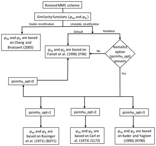
Note that all the functions stated above have been newly installed in the revised MM5 surface layer scheme of WRFv4.2.2 and can be used in place of F96 functions already employed in the model. Here, we have introduced a new surface layer module where different options for φ_m and φ_h can be controlled using an appropriate value of the namelist parameter (psimhu_opt). The parameter psimhu_opt is added under the physics section of the namelist file. The variable psimhu_opt can have values 0, 1, 2, and 3 for different options for functions F96 (default), BD71, CL73, and KY90, respectively. A brief structure and different choices for psimhu_opt based on newly installed and default functional forms of φ_m and φ_h in the default and modified revised MM5 scheme are shown in Fig. 1.

Figure 1 Flowchart to provide a brief description of different options for similarity functions in the modified surface layer scheme that can be controlled by namelist variable psimhu_opt.

2.3 Characteristics of default and newly installed similarity functions

The expressions of φ_m and φ_h for different functional forms utilized in this study are stated in Appendix A. Figure S1 in the Supplement shows the variation in different (a) φ_m and (b) φ_h under moderately to strongly unstable conditions. It is evident from Fig. S1 that all the different functional forms provide similar values of φ_m and φ_h in near-neutral to moderately unstable conditions (up to $\mathit{\zeta }=-\mathrm{0.1}$ approximately). However, at higher instabilities one can expect noticeable differences between different functional forms of φ_m and φ_h. Note that the functional forms for φ_m corresponding to BD71 and CL73 decrease continuously with increasing instability; however, φ_m corresponding to KY90 functional forms shows decreasing behavior in near-neutral to moderately unstable conditions and attains a minimum at $\mathit{\zeta }=-\mathrm{1.574}$, and, as the instability further increases, it starts increasing with −ζ (Fig. S1a). This implies that φ_m based on class 4 functions shows non-monotonic behavior which contradicts the classical MOST prediction. On the other hand, in the case of φ_h, all the functional forms provide continuously decreasing behavior of φ_h from near-neutral to moderately unstable conditions (Fig. S1b).

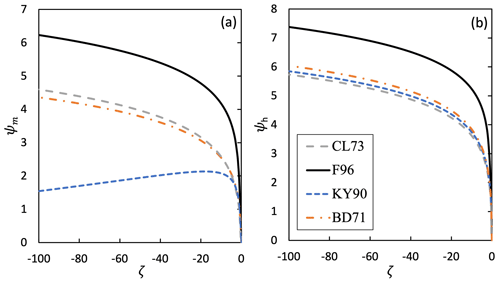
Figure 2 Integrated similarity functions ψ_m,h(ζ) for momentum and heat for default (F96; black line) and newly installed (BD71, CL73, and KY90; orange, gray, and blue lines, respectively) functions for unstable atmospheric surface layer.

Figure 2 illustrates the variation in default (F96) and newly installed integrated similarity functions ψ_m and ψ_h (BD71, CL73, and KY90) with respect to −ζ. One can see from Fig. 2a that ψ_m corresponding to F96, BD71, and CL73 functional forms increases continuously with −ζ in moderately to strongly unstable conditions. However, a non-monotonic behavior has been found for ψ_m corresponding to the KY90 functions implying it first increases with −ζ and reaches a maximum at $\mathit{\zeta }=-\mathrm{1.574}$ and then starts decreasing as instability further grows. On the other hand, ψ_h corresponding to all the considered functional forms increases continuously in near-neutral to strongly unstable conditions. However, the rate of increase is slightly higher for F96 in comparison to the other three functions (BD71, CL73, and KY90), whose results are very similar to each other (Fig. 2b).

2.4 Observational data for model evaluation

For the evaluation of different simulations corresponding to newly installed similarity functions, observational data derived from the micrometeorological tower installed at Ranchi (India) have been utilized (Srivastava and Sharan, 2019; Srivastava et al., 2020, 2021). The dataset (Ranchi data) is derived from an instrument mounted on a 32 m tall tower at the Birla Institute of Technology Mesra in Ranchi, India (Dwivedi et al., 2015), with an average elevation of 609 m above sea level in a tropical region. The site has a few buildings in between the east and northwest, agricultural land in between the northwest and west, and a residential area and dense trees in between the southeast and east. The site also has a relatively flat area in between southeast and west which is free from any obstacle (Srivastava and Sharan, 2015). A fast response sensor (CSAT3 sonic anemometer) at a height of 10 m with an average elevation 609 m above sea level provides the temperature and the three components of wind at a 10 Hz frequency. The eddy covariance technique (Stull, 1988) is used to estimate heat and momentum fluxes at 1 h time resolution; however the hourly temperature at 2 m is determined by averaging temperature observations available at a temporal scale of 1 min from the slow response sensors located at logarithmic heights on the same tower. We have utilized hourly data for considered variables. Apart from this we have also utilized the ERA5-Land reanalysis dataset available at 0.10° × 0.10° spatial resolution to evaluate the spatial distribution of the model-simulated near-surface atmospheric variables. For consistency, we have regridded the model output to the same grid resolution of the reanalysis and observed datasets.

3 Numerical simulations

To analyze the impacts of newly installed similarity functions together with the existing functional forms in the surface layer scheme of WRFv4.2.2, the performance of the default and newly installed similarity functions is investigated in two steps. The first one is independent of the WRF model. Namely, we apply Eq. (B8) (Appendix B) to iteratively determine C_D and C_H as a function of ζ by prescribing the bulk Richardson number (Ri_B) and surface roughness parameters for momentum (z₀) and heat (z_h). The value of ζ is estimated by calculating the root of least magnitude of Eq. (B8) for a given value of Ri_B. Once ζ is calculated and then utilizing it in Eqs. (B9) and (B10), the values of C_D and C_H can be estimated. We call this in the following the offline simulation. For the computation, z is taken as 10 m and Ri_B is in the range $-\mathrm{2}\le {\mathit{Ri}}_{\mathrm{B}}\le \mathrm{0}$. The offline simulations are carried out over three different surface types by considering surface roughness (z₀) to be 0.01 m (smooth surface), 0.1 m (transition surface), and 1 m (rough surface) to analyze the impact of the roughness of the underlying surface on the simulation of ζ, C_D, and C_H.

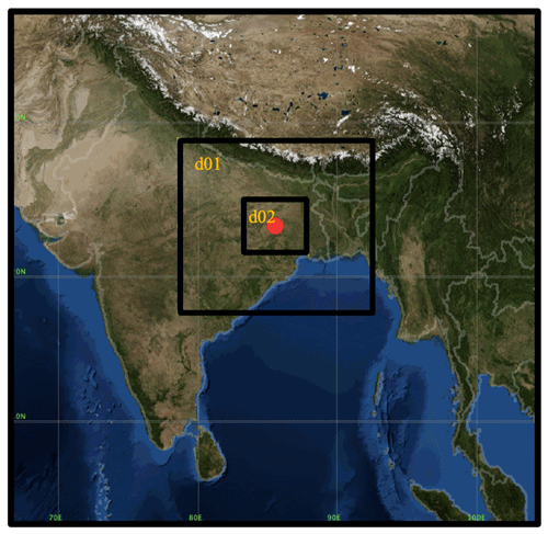
Figure 3 Spatial distribution of domain used for the simulations using the WRF model. The spatial resolution for domains d01 and d02 is 6×6 and 2×2 km², respectively. The domain d02 covers an area of 446×392 km² around the center point.

The second step is to apply all the parameterizations of the similarity functions in the WRF model version 4.2.2 over an Indian land site whose output is compared then with the observations during the pre-monsoon (March–April–May; MAM) season of the year 2009. The simulations have been conducted over a nested domain centered around the location of a micrometeorological tower installed at Ranchi (23.412° N, 85.44° E), India (Fig. 3). Domain d01 (6×6 km²) consists of 233 east–west and 210 north–south grid points, and domain d02 (2×2 km²) consists of 223 east–west and 196 north–south grid points which cover a 1398×1260 and a 446×392 km² spatial area around the center point, respectively. Each domain was configured with 50 vertical eta levels from the surface to the top of the atmosphere. We kept five vertical levels below 100 m height. Initial and boundary conditions were taken from an ERA5 global atmospheric reanalysis dataset at a resolution of 0.25° × 0.25°, and boundary conditions were forced every 6 h. For land use and land cover (LU/LC) information, we have used a dataset from MODIS (Moderate Resolution Imaging Spectroradiometer; Friedl et al., 2002). Various physical parameterizations utilized in the simulations are listed in Appendix C. In this study, four sets of simulations were carried out, as given in Table 1.

Table 1 Description of various simulations conducted in this study.

Note that the revised MM5 surface layer scheme has lower limits on the values of u_∗ (>0.001 m s⁻¹) and U (>0.1 m s⁻¹) that allow nocturnal values of u_∗ at night and control Ri_B values to be inordinately high, respectively (Jiménez et al., 2012). However, the stability parameter ζ or Ri_B is not restricted in the revised MM5 surface layer scheme, which gives complete freedom to the WRF model to show its sensitivity to the tested similarity functions (Jiménez et al., 2012). Moreover, some of the large-eddy simulation (LES) studies reported in the literature suggest that the friction velocity cannot be zero when the mean wind drops to zero; i.e., there should be a minimum friction velocity that is proportional to the w_∗ (Schumann, 1988). For this purpose, the existing version of the revised MM5 scheme sets 0.001 m s⁻¹ as the minimum value of u_∗ based on the recommendations by Jiménez et al. (2012). Thus, to avoid the complexity that arises when mean wind drops to zero, the updated revised MM5 scheme proposed in the present study also utilizes a minimum value of u_∗ (>0.001 m s⁻¹) as suggested by Jiménez et al. (2012) in the existing version of the revised MM5 scheme. Moreover, the scheme uses constant values of z₀, while the values of z_h are calculated from the expression suggested by Brutsaert (1982).

The whole simulation period is divided into segments of 4 d with 24 h overlapping time between different segments to ensure continuity. The model is initialized at 00:00 UTC of the first day of each simulation and runs for 96 h. In order to avoid the potential spin-up problems at the beginning of the simulation, we discard the first day of each simulation as spin-up time and consider the last 3 d for the analysis (Jiménez et al., 2010, 2012).

For the evaluation of the real-case simulations, different statistical parameters such as mean absolute error (MAE), root mean square error (RMSE), mean bias (MB), index of agreement (IOA), different measures of correlation coefficient (CC), mean bias percent (bias %), and standard deviation of the model-predicted output normalized by that of the observations are used. A brief description of the performance indicators for validation utilized in the present study is given in Appendix C.

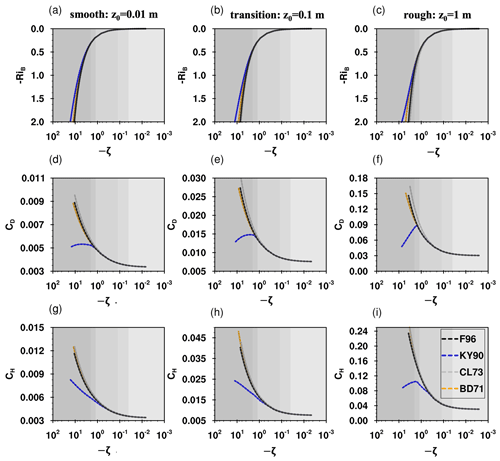
Figure 4 Variation in ζ with Ri_B (a–c), C_D (d–f), and C_H (g–i) with ζ calculated from the bulk flux algorithm (offline simulation) for different functional forms of ψ_m and ψ_h corresponding to BD71, CL73, KY90, and F96 forms for smooth (z₀=0.01 m; a, d, g), transition (z₀=0.1 m; b, e, h), and rough (z₀=1.0 m; c, f, i) surfaces. The background color corresponds to different sublayers in convective conditions (Kader and Yaglom, 1990), from the dynamic sublayer ($\mathrm{0}\ge \mathit{\zeta }>-\mathrm{0.04}$; light gray) to the free convective sublayer ($\mathit{\zeta }<-\mathrm{2}$; dark gray).

4 Results

4.1 Offline simulations

To analyze the functional dependence of ζ, C_D, and C_H on the utilized forms of similarity functions, the offline simulations independent of the WRF model have been conducted utilizing newly installed functions (BD71, CL73, and KY90) together with F96 functions existing in the default version of the surface layer scheme of the WRF model for three different roughness lengths for momentum (z₀), which are representative of smooth (z₀=0.01 m), transition (z₀=0.1 m), and rough ( z₀=1.0 m) surfaces. The results for ζ (Fig. 4a, b, and c) with Ri_B, C_D (Fig. 4d, e, and f), and C_H (Fig. 4g, h, and i) with ζ across various surface types and sublayers have been analyzed. The different sublayers associated with convective stratification include dynamic (DNS), dynamic and dynamic convective transition (DNS-DCS), dynamic convective (DCS), dynamic convective and free convective transition (DCS-FCS), and free convective (FCS) (Srivastava and Sharan, 2021). Note that the sublayers DNS ($-\mathrm{0.04}\le \mathit{\zeta }\le \mathrm{0}$) and DNS-DCS transition ($-\mathrm{0.12}\le \mathit{\zeta }<-\mathrm{0.04}$) correspond to weakly to moderately unstable conditions, while sublayers DCS ($-\mathrm{1.20}\le \mathit{\zeta }<-\mathrm{0.12}$), DCS-FCS ($-\mathrm{2.0}\le \mathit{\zeta }<-\mathrm{1.20}$), and FCS ($\mathit{\zeta }<-\mathrm{2.0}$) belong to moderately to strongly convective conditions (Srivastava and Sharan, 2015).

It is found that the simulated values of ζ at smaller values of Ri_B (i.e., in DNS to DCS) from different forms of similarity functions are almost identical to the F96 functional forms (Fig. 4a–c). Moreover, results from the BD71, CL73, and F96 functions are even similar at higher instabilities (i.e., the whole range of ζ values), while they differ strongly from values obtained using the KY90 functions (Fig. 4a–c). Notably, BD71, CL73, and F96 functional forms predict relatively smaller absolute values of ζ for a given value of Ri_B. However, KY90 functions are found to produce a relatively larger magnitude of ζ for a given value of Ri_B. This behavior is found to be consistent for all ratios $z/z_{\mathrm{0}}$ (Fig. 4a–c) representative of smooth, transition, and rough surfaces. A relatively larger magnitude of ζ for a given value of Ri_B and the smaller values of ψ_m and ψ_h (Fig. 2) in KY90 functional forms imply that the momentum and heat fluxes predicted using KY90 functions will be smaller than those anticipated in BD71, CL73, and F96 functional forms.

Figure 4d–f show the variation in C_D with ζ estimated using BD71, CL73, KY90, and F96 functional forms over different surfaces. Notice that the C_D values calculated from BD71, CL73, and F96 forms of functions are relatively higher than those produced by KY90 functional forms and continue to rise as instability progresses from DCS to FCS. It is important to highlight that C_D estimated using KY90 functions shows a non-monotonic behavior, which is consistent with the observed behavior of C_D over the Indian region reported in the literature (Srivastava and Sharan, 2019, 2021). Note that this non-monotonic behavior is consistent for all three cases of different roughness lengths (Fig. 4d–f).

On the other hand, across all three surfaces, one can see that the values of C_H estimated from all four functional forms increase with increasing instability (Fig. 4g–i), while the rate of increase of C_H in KY90 functions is relatively slower. Moreover, BD71, CL73, and F96 functions predict almost similar values over all three types of surfaces. Noticeably, C_H estimated using KY90 functions also exhibits non-monotonic behavior with ζ over rough surfaces, which contradicts the predictions of the other three functional forms. In addition, it is important to note that C_D and C_H predicted by KY90 functional forms are found to be bounded by twice their near-neutral values, while the other functional forms predict continuously increasing values of C_D and C_H with increasing instability.

Note that the error caused by different values of z₀ can be so large that the stability dependence of using different forms of similarity functions is less important in the computation of C_D and C_H. As a result, three different values of z₀ have been chosen, similar to a recent study by Srivastava and Sharan (2021), which are representative of smooth (z₀=0.01 m), transition (z₀=0.1 m), and rough (z₀=1.0 m) surfaces to account for the impacts of using different z₀ on the estimation of C_D and C_H from different functional forms of similarity functions in offline simulations.

Moreover, Fig. 4 depicts the offline simulations with equal values of z₀ and z_h, while in the revised MM5 surface layer scheme available in the WRF model, the values of z₀ and z_h are not the same. Thus, we have also attempted to discuss the results from the offline simulations with different values of z_h, assuming z₀=0.1 m. Figure S2 shows the variation in ζ with Ri_B, C_D, and C_H with ζ calculated from the bulk flux algorithm using similarity functions corresponding to BD71, CL73, KY90, and F96 with different values of z_h while z₀ is fixed. The values of z_h are taken such that the ratio $\ln (z_{\mathrm{0}}/z_{\mathrm{h}})$ assumes 0.1, 1, 2, 3, and 4. Figure S2 clearly shows that the estimated values of ζ are similar in near-neutral to moderately unstable conditions for all values of z_h; however, relatively smaller values have been found as the ratio $\ln (z_{\mathrm{0}}/z_{\mathrm{h}})$ increases for each form of similarity function. Since the computation of C_D does not involve the values of z_h (Eq. B9), the estimated values of C_D for each form of similarity function are found to be approximately the same for different values of z_h. However, in the case of C_H, differences are clearly visible if one uses different values of z_h. The estimated C_H using various similarity functions behaves similarly for different values of z_h, while the magnitude decreases as the ratio $\ln (z_{\mathrm{0}}/z_{\mathrm{h}})$ increases.

Hence, it is evident that the BD71, CL73, and F96 functional forms predict values of ζ, C_D, and C_H that are almost the same over all three different surface types. However, using KY90 functions compared to other commonly used φ_m and φ_h, one can expect a significant reduction in the estimated values of transfer coefficients in moderately to strongly unstable stratification.

4.2 Results of the WRF model using different sets of integrated similarity functions

In this section, observational and reanalysis datasets have been used to analyze the simulations performed with WRFv4.2.2 utilizing newly installed and default φ_m and φ_h. The model-simulated output has been extracted at the location of the flux tower and compared against the observations derived from the flux tower installed at Ranchi (23.412° N, 85.440° E), India. The mean spatial patterns of certain variables averaged over daytime (04:00–12:00 UTC) have been compared against the ERA5-Land reanalysis dataset. Further, to assess the effects of newly installed functions under free convective conditions, the mean spatial patterns of considered variables averaged across strongly convective conditions (hours in which $\mathit{\zeta }<-\mathrm{10}$ over most of the domain) have been analyzed against respective hours of ERA5-Land reanalysis data. Bilinear interpolation has been used to interpolate the model output to the same grid resolution as the ERA5-Land data in order to allow a consistent comparison.

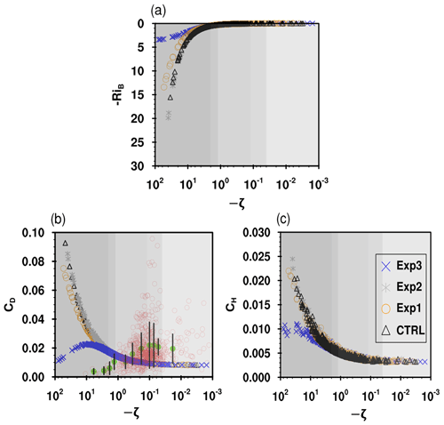
Figure 5 Variation in model-simulated ζ with Ri_B (a), C_D (b), and C_H (c) with ζ from different experiments using different ψ_m and ψ_h corresponding to F96 (CTRL), BD71 (Exp1), CL73 (Exp2), and KY90 (Exp3) under convective conditions. The red circles in (b) denote the observed C_D with ζ at the location of the flux tower. The mean values of observed C_D in each sublayer are shown with solid green circles along with standard deviations in the form of error bars. Depending upon the data availability, two or three bins of equal width are chosen in each sublayer. The background color corresponds to different sublayers in convective conditions (Kader and Yaglom, 1990), from the dynamic sublayer ($\mathrm{0}\ge \mathit{\zeta }>-\mathrm{0.04}$; light gray) to the free convective sublayer ($\mathit{\zeta }<-\mathrm{2}$; dark gray).

4.2.1 Evaluation against observations derived from the flux tower installed at Ranchi (India)

Figure 5 depicts the variation in (a) ζ with Ri_B, (b) C_D, and (c) C_H at the first model level with ζ from different experiments (Exp1, Exp2, and Exp3) and the CTRL simulation. Although the absolute values of the parameters differ from each other due to the different prescribed roughnesses, the variation in ζ with Ri_B, C_D, and C_H with ζ is very similar to the offline results. Note that, at the moment, due to the inaccessibility of long-term data on detailed surface properties such as vegetation structure needed to quantify the roughness length, we do not have access to the precise values of z₀ and z_h at the Ranchi station. Moreover, the values of z₀ and z_h are not directly involved in the estimation of C_D, C_H, and the surface fluxes from the observational data, while they are important in computing these variables using the MOST framework. Thus, the default value of z₀ is used in the revised MM5 surface layer scheme available in the WRF model, which is found to be approximately in the range 0.1–0.2 m at the Ranchi station. We wish to highlight that the z₀ used in the WRF model simulations at the Ranchi station is nearly similar to the case of z₀=0.1 m presented in Fig. 4, and the offline simulations also indicate that the behavior of the estimated C_D and C_H with ζ remains almost the same for different values of z₀ with slightly varying magnitudes. Thus, one can interpret the results of C_D and C_H shown in Figs. 4 and 5 from the offline simulations and the WRF model, respectively, and can compare the WRF-model-simulated C_D with the observed one at the Ranchi station. Although the model simulations and observed data may have a different z₀, the comparison of model-simulated variables with the Ranchi data allows for an impression of the structural behavior of model results as a function of stratification compared with measurements.

It is clear from Fig. 5 that the values of simulated variables are found to be almost identical in DNS to DCS sublayers for all the experiments. Moreover, in FCS, the results obtained from Exp1, Exp2, and the CTRL simulation are found to be nearly similar; however, relatively strong differences have been found in results from Exp3 (Fig. 5a, b, and c). Simulated ζ for a given Ri_B in Exp2 and the CTRL simulation are similar and found to be relatively smaller in magnitude than Exp1 and Exp3 in FCS. However, the absolute values of ζ in Exp3 (KY90 functions) are relatively higher in FCS than in all other experiments.

Figure 5b shows the variation in simulated C_D with ζ from different experiments. Purple circles denote the variation in observed C_D with ζ at the location of the flux tower (Fig. 5b). It is found that the observed C_D increases as the instability increases from DNS to DCS and has the maximum value in the DCS (at $\mathit{\zeta }=-\mathrm{0.1}$ approx.) and then starts to decrease as instability grows further from DCS to FCS. It is evident that C_D simulated using φ_m and φ_h based on class 4 functions (Exp3) exhibits non-monotonic behavior (Fig. 5b), which is consistent with the observed behavior of C_D (Srivastava and Sharan, 2015, 2021). The magnitude of C_D predicted in Exp3 is significantly smaller than that simulated from other experiments as well as the CTRL simulation, specifically in FCS. This may be due to the large differences between the KY90 functional forms of ψ_m and ψ_h and other forms of functions. On the other hand, C_D simulated using φ_m and φ_h based on the first three classes (Exp1, Exp2, and CTRL simulation) increases continuously as instability grows from DNS to FCS (Fig. 5b).

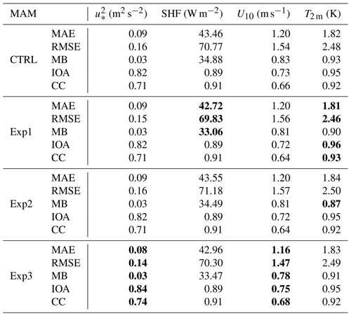
Table 2 Comparison statistics for $u_{\ast }^{\mathrm{2}}$ (m² s⁻²), sensible heat flux (SHF) (W m⁻²), U₁₀ (m s⁻¹), and T_2 m (K) simulated using different experiments together with the CTRL simulation with respect to observations derived from the flux tower at Ranchi (India) for the MAM season. The mean absolute error (MAE), root mean square error (RMSE), mean bias (MB), index of agreement (IOA), and correlation coefficient (CC) are shown. The highest (lowest) values of CC and IOA (MAE, RMSE, and MB) between different experiments are denoted by bold entries.

However, it is found that C_D predicted from the original forms of class 4 functions (Exp3) shows a large disagreement with its observed behavior, as the predicted C_D starts decreasing at ζ lying in FCS, which is different from that observed, i.e., ζ lying in DCS. As a result, the study also highlighted the necessity of fine-tuning the original KY90 functional forms and evaluating their performance in the WRF model with additional observational datasets from various land sites and seasons.

Note that Srivastava and Sharan (2021) tuned the original forms of class 4 functions by enforcing the matching of the point at which both observed and model-predicted C_D attain their maximum value. However, more studies in terms of predicting the observed variation in the non-dimensional vertical gradients of mean wind speed and temperature with ζ are essential to further tune the original KY90 functions for the Indian region using observed data from various locations under different seasons.

Further, we would like to point out that currently no observational datasets are available which show a better agreement with the KY90 functions over the Indian region. However, it is desirable to further validate these functional forms over the Indian region once such observational datasets become available.

We wish to highlight that utilizing KY90 (Exp3) functions in the revised MM5 scheme of the WRF model makes it consistent in predicting C_D with its observed non-monotonic behavior over the Indian region.

The variation in simulated C_H with ζ from different experiments is shown in Fig. 5c. C_H simulated from Exp1–3 as well as the CTRL simulation shows continuously increasing behavior with ζ. The magnitude of simulated C_H from the CTRL simulation and Exp1–2 is relatively higher than that of Exp3 in FCS beyond $\mathit{\zeta }<-\mathrm{10}$ (approximately). It is also evident that at higher instabilities, even C_H shows non-monotonic behavior with ζ (Fig. 5c). We wish to point out that a relatively larger scatter has been found in the values of C_H than C_D. The WRF model utilizes constant values for z₀, while z_h is calculated using expression suggested by Brutsaert (1982). The relatively large scatter in the values of C_H simulated from the WRF model can be due to the parameterization of the ratio of momentum and scalar roughness lengths in the model.

Note that the transfer coefficients C_D and C_H shown in Fig. 5 are at the reference height corresponding to the lowest model grid level, which is ∼12 m in the present study. However, we have also analyzed the behavior of C_D and C_H at 10 m height with ζ and found that they behave similarly to those presented in Fig. 5.

The analysis presented here indicates that the KY90 functions in the revised MM5 surface layer scheme are found to be appropriate in producing non-monotonic behavior of C_D consistent with its observed nature. However, all other functional forms of φ_m and φ_h produce C_D, which increases continuously with ζ from DNS to FCS.

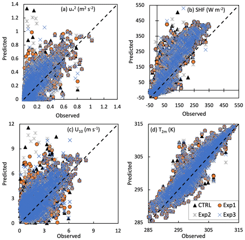
Figure 6 Scatter plot of model-simulated $u_{\ast }^{\mathrm{2}}$ (representative of momentum flux) (a), SHF (sensible heat flux) (b), U₁₀ (wind speed at 10 m height) (c), and T_2 m (temperature at 2 m height) (d) vs. observed values at the location of the flux tower at Ranchi (23.412° N, 85.440° E), India, during the pre-monsoon season (MAM).

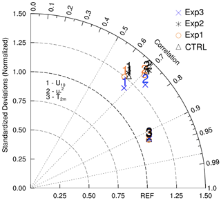
Figure 7 Taylor diagram showing the correlation coefficient and normalized standard deviations for U₁₀, $u_{\ast }^{\mathrm{2}}$, and T_2 m from different experiments together with the CTRL simulation with respect to observations derived from the flux tower installed at Ranchi (23.412° N, 85.440° E), India.

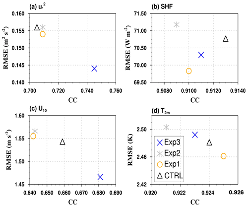
Figure 8 Scatter plot between correlation coefficient (CC) and root mean square error (RMSE) for $u_{\ast }^{\mathrm{2}}$ (a), SHF (b), U₁₀ (c), and T_2 m (d) simulated by various experiments (Exp1–3) together with the CTRL simulation for the pre-monsoon season (MAM) at the location of the flux tower at Ranchi (23.412° N, 85.440° E), India.

To quantify the uncertainties involved in the simulated surface fluxes and certain near-surface variables using KY90 (Exp3) as well as other functional forms (Exp1–2 and CTRL simulation), model simulations have been compared against the observations. Figure 6 compares the model-simulated (a) $u_{\ast }^{\mathrm{2}}$ (m² s⁻²) (representative of momentum flux), (b) SHF (W m⁻²) (sensible heat flux), (c) U₁₀ (m s⁻¹) (10 m wind speed), and (d) T_2 m (K) (2 m temperature) with the observed data obtained from the flux tower at Ranchi (23.412° N, 85.440° E), India. The model output was extracted at a single grid point closest to the flux tower to allow a consistent comparison. In Fig. 7, a Taylor diagram is displayed along with the normalized standard deviations and correlations of considered variables. Figure 8 shows the scatter plot between CC and RMSE for considered variables simulated using different experiments. In the case of $u_{\ast }^{\mathrm{2}}$, Exp1 and Exp2 are found to be comparable to the CTRL simulation, while Exp3 considerably improved the simulation of $u_{\ast }^{\mathrm{2}}$ (Figs. 6a, 7 and 8). Exp3 reduced MAE (RMSE) from 0.09 (0.16) m² s⁻² to 0.08 (0.14) m² s⁻² (Table 2; Figs. 7 and 8) and improved the CC (0.74) and IOA (0.84) for $u_{\ast }^{\mathrm{2}}$ (Table 2). A Q–Q plot is shown in Fig. S3a suggesting that Exp3 (KY90 functions) is found to be slightly better than all other experiments and the CTRL simulation for $u_{\ast }^{\mathrm{2}}$. For SHF, all the experiments are comparable to the CTRL simulation; however, Exp3 shows less scatter than other experiments (Fig. 6a).

In the case of U₁₀, Exp3 shows less scatter and appears to be closer to the observations than other experiments (Fig. 6c). Exp3 noticeably improved the simulation of U₁₀ by reducing MAE (RMSE) from 1.20 (1.54) m s⁻² to 1.16 (1.47) m s⁻² and MB up to 5 % (Figs. 6c, and 7; Table 2). It considerably improved the CC (IOA) for U₁₀ from 0.66 (0.73) to 0.68 (0.75) (Fig. 7 and Table 2). A Q–Q plot (Fig. S3b) reveals that Exp3 is found to be better than all other experiments and the CTRL simulation for U₁₀. Thus, the KY90 functions in the surface layer scheme of the WRF model considerably improve the model in simulating U₁₀ (Figs. 6c, 7, 8, and S2b) at the location of the flux tower. Further, in the case of T_2 m, Figs. 7 and 8 show that all the experiments are found to be comparable with the CTRL simulation.

Note that earlier studies, especially the ones done in the GEWEX Atmospheric Boundary Layer Study (GABLS) model intercomparison projects, have studied the impacts of the similarity functions on the modeled profiles and fluxes (though mostly for stable conditions). However, they learned that applying different stability functions in the surface and boundary layer parameterizations may trigger unnatural kinks in the model-simulated wind speed and temperature profiles. Here, we have analyzed the profiles of U₁₀ and T_2 m simulated from the WRF model using different similarity functions in the surface layer scheme for the occurrence of unnatural kinks in their values. One can see that the U₁₀ predicted from the CTRL simulation, as well as different experiments corresponding to different similarity functions at certain hours, goes higher than that of its observed maximum value (approx. 8 m s⁻¹) (Fig. S4). These relatively higher magnitudes may be linked with some localized weather phenomenon characterized by rapid changes in weather including strong wind, lightning, and thunderstorms and are justifiable. However, the simulated T_2 m from different similarity functions are found to be in line with the observed values across the whole simulation period (Fig. S5). This suggests that the values of U₁₀ and T_2 m predicted from the WRF model are found to be in a justifiable range and no unnatural kinks have been found.

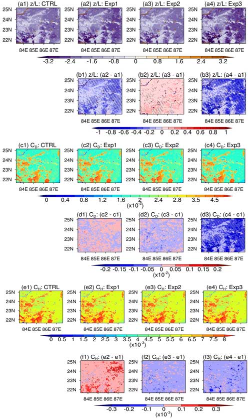
Figure 9 Mean spatial distribution of model-simulated ζ (a), C_D (c), and C_H (e) from different experiments and their differences (b, d, f) with respect to the CTRL simulation averaged during daytime for the whole simulation period. Hatched regions show significant differences at 95 % confidence level in experiments with respect to the CTRL simulation.

4.2.2 Evaluation of mean spatial distribution of simulated variables against ERA5-Land reanalysis data during daytime

In this section, the mean spatial distribution of simulated variables from different experiments, as well as the CTRL simulation averaged during daytime (04:00–12:00 UTC) for the entire simulation period, is compared with the ERA5-Land reanalysis data. Figure 9 depicts the mean spatial patterns of simulated $\mathit{\zeta }\left(=\frac{z}{L}\right)$ (a1–a4), C_D (c1–c4), and C_H (e1–a4) from the CTRL simulation and other experiments, as well as their differences with respect to the CTRL simulation. It is found that the absolute value of ζ simulated in Exp3 (KY90 functions) is relatively smaller than the CTRL simulation (Fig. 9b3) across the whole domain, which is consistent with Fig. 5a, and offline simulations presented in Fig. 4a–c. This could be because the magnitude of KY90 functions (φ_m and φ_h) (Fig. S1) is relatively smaller than the functions employed in the default scheme (CTRL simulation).

On the other hand, Exp1 also provides slightly smaller absolute values of ζ (Fig. 9b1), while Exp2 is almost comparable to the CTRL simulation (Fig. 9b2). Model-simulated C_D is found to be relatively smaller in Exp3 than the CTRL simulation (Fig. 9d3), while Exp1 and Exp2 provide comparable values of C_D to the CTRL simulation (Fig. 9d1–2). In the case of C_H, the simulated values from different experiments are comparable to the CTRL simulation over the whole study domain (Fig. 9f1–3). Note that simulated C_H is found to be comparable in all the experiments, while one can see slight differences in C_D in Exp3 compared to all other experiments, which may be related to the fact that only φ_m functions are involved in the computation of C_D (Eq. 1) and the differences between φ_m corresponding to Exp3 are relatively more than φ_h, as are the differences in C_D. The hatched regions in Fig. 9 show that the differences between simulated variables from different experiments with respect to the CTRL simulation are statistically significant at 95 % confidence level.

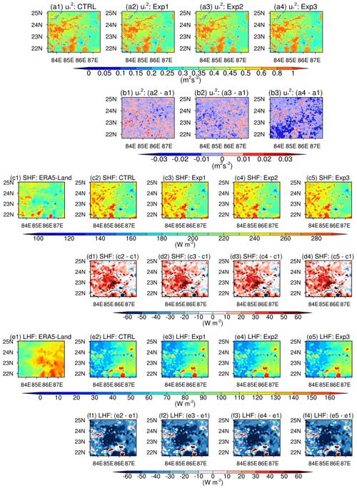
Figure 10 Mean spatial distribution of simulated $u_{\ast }^{\mathrm{2}}$ (a) from different experiments and their differences (b) with respect to the CTRL simulation. SHF (c) and LHF (e) from ERA5-Land reanalysis and simulated using various experiments and their differences (d, f) with respect to ERA5-Land data averaged during daytime for the whole simulation period are shown. Hatched regions show significant differences at 95 % confidence level in experiments with respect to the CTRL simulation.

The slight differences in C_D in Exp3 are reflected further in the simulated $u_{\ast }^{\mathrm{2}}$ m² s⁻² (a measure of momentum flux) (Fig. 10b3). A slight reduction has been found in simulated $u_{\ast }^{\mathrm{2}}$ in Exp3 compared to the CTRL simulation over some parts of the domain (Fig. 10b3), while in Exp1 and Exp2 values are comparable with the CTRL simulation (Fig. 10b1–2). In the case of SHF and latent heat flux (LHF), the mean spatial distribution from all the experiments is found to be consistent with the ERA5-Land reanalysis data, and the magnitude of differences between model simulation and ERA5-Land data is comparable for all the experiments (Table S1 in the Supplement).

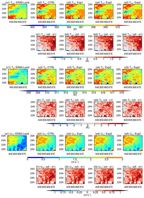
Figure 11 Mean spatial distribution of T_2 m (upper panels), T_S (middle panels), and U₁₀ (lower panels) from ERA5-Land reanalysis (a1, c1, e1, respectively) and different experiments (a2–a5, c2–c5, e2–e5, respectively) and their differences with respect to ERA5-Land reanalysis (b1–b4, d1–d4, f1–f4, respectively) averaged during daytime for the whole simulation period.

For T_2 m (upper panels of Fig. 11), T_S (middle panels of Fig. 11), and U₁₀ (lower panels of Fig. 11), the mean spatial distribution from different experiments and the CTRL simulation agreed well with slightly varying magnitude with the ERA5-Land reanalysis data. One can see a warm bias up to 2 K (3 K) for T_2 m (T_S) simulated from different experiments and the CTRL simulation over most of the domain. For T_2 m, bias, RMSE, and pattern correlation coefficient (PCC) between different experiments together with the CTRL simulation and ERA5-Land reanalysis data are found to be comparable (Table S1). However, Exp3 slightly improved the PCC from 0.50 to 0.51 for T_S (Table S1). Further, in the case of U₁₀, all the simulations exhibit an overprediction over the whole domain (lower panels of Fig. 11: f1–f4), and Exp3 is found to be slightly better than all other experiments as well as the CTRL simulation as it reduced bias % (RMSE) from 32.28 (0.54) m s⁻² to 32.06 (0.53) m s⁻² and improved the PCC from 0.89 to 0.91 (Table S1).

4.2.3 Evaluation of newly installed functions during strongly unstable conditions with respect to ERA5-Land reanalysis data

This section describes the impacts of utilizing different similarity functions (φ_m and φ_h) on simulated variables during highly convective regimes (i.e., $\mathit{\zeta }<-\mathrm{10}$) with respect to the ERA5-Land reanalysis dataset. Since the functional forms of ψ_m and ψ_h are almost identical in near-neutral to moderately unstable conditions, however, in strongly unstable conditions, the differences between different functional forms are more pronounced. Thus, the corresponding differences in the simulated values of considered variables are expected to be more pronounced during highly convective regimes. For this purpose, the model output has been extracted for those hours in daytime which show ζ smaller than −10 over most of the domain and compared with the respective hours of ERA5-Land reanalysis data.

Figure S6 depicts the mean spatial distribution of ζ (a1–4), C_D (c1–4), and C_H (e1–4) as well as their deviations from the CTRL simulation. Notice that the magnitudes of differences for all variables (ζ, C_D, and C_H) in this case are found to be larger than the case of mean spatial patterns averaged during the whole daytime (Sect. 6.2.2). It is evident from Fig. S6b3 that Exp3 produces large absolute values of ζ and smaller values of C_D and C_H (Fig. S6b3, d3, and f3) than all other experiments and the CTRL simulation, while Exp1 and Exp2 are found to be comparable to the CTRL simulation for both C_D and C_H (Fig. S6d1–2 and f1–2).

Table 3 Comparison statistics for T_2 m (K), T_S (K), and U₁₀ (m s⁻¹) simulated using different experiments together with the CTRL simulation with respect to ERA5-Land reanalysis data averaged during strongly unstable stratification (hours during daytime in which ζ is smaller than −10) for the whole simulation period. The mean bias percent (bias %), pattern correlation coefficient (PCC), and root mean square error (RMSE) are shown. The lowest (highest) values of bias and RMSE (PCC) between different experiments are denoted by bold entries.

The model simulations for T_2 m and T_S do not capture the spatial patterns well in comparison to ERA5-Land data (Figs. S7a1–5 and S8a1–5). All experiments, as well as the CTRL simulation, exhibit an overprediction across the whole domain (Figs. S7b1–4 and S8b1–4). We wish to highlight that the differences between various experiments and the CTRL simulation are seen up to 0.5 K for T_2 m (Fig. S7c1–3) as well as T_S (Fig. S8c1–3), which is slightly higher than the case of mean spatial patterns averaged over the whole daytime (upper and middle panels of Fig. 11). For T_2 m, it is evident from Fig. S7 and Table 3 that Exp3 noticeably reduced the bias % (RMSE) from 0.64 (2.13) K to 0.62 (2.10) K and improved the PCC from 0.43 to 0.46 (approximately 6 %). In the case of T_S as well, Exp3 slightly improved the PCC and reduced the bias % (RMSE) from 1.25 (4.01) K to 1.24 (3.97) K (Table 3 and Fig. 12).

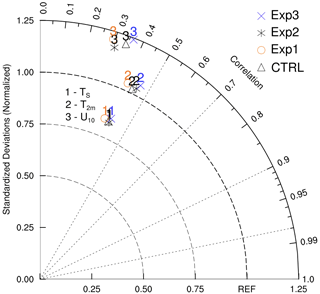
Figure 12 Taylor diagram showing the correlation coefficient and normalized standard deviations for T_S (K), T_2 m (K), and U₁₀ (m s⁻¹) from different experiments together with the CTRL simulation with respect to the ERA5-Land reanalysis dataset averaged during strongly convective conditions (hours during daytime in which ζ is smaller than −10) for the whole simulation period.

For U₁₀, the mean spatial patterns simulated using different experiments agreed well with the ERA5-Land reanalysis data (Fig. S9a1–5), and the magnitude of biases is found to be up to 1 m s⁻¹. Exp3 outperformed all other experiments and the CTRL simulation by lowering the bias % from −4.96 to −0.28 m s⁻¹ and improved the PCC from 0.34 to 0.36 with comparable RMSE values (Figs. S9 and 12; Table 3).

The results presented so far suggest that the changes corresponding to different functional forms of similarity functions in the surface layer parameterization of the WRF model are more pronounced in convective conditions during daytime hours. For the number of grid points over the study domain that are being affected by the changed similarity functions, no fixed pattern was found; however, the changes depend on the considered variable and similarity functions. Furthermore, we observe that the changes are more pronounced in grids that experience strong instability during the daytime.

5 Summary and concluding remarks

In the present study, the revised MM5 surface layer scheme of the WRFv4.2.2 model has been modified to incorporate φ_m and φ_h as suggested by Kader and Yaglom (1990) to make it consistent in producing the transfer coefficient for momentum (C_D) in line with its observed behavior. The revised MM5 scheme is modified in such a way that it contains all commonly used φ_m and φ_h under convective conditions instead of a single functional form. Various alternatives of φ_m and φ_h in the modified scheme can be controlled by a flag (psimhu_opt) that has been introduced in the physics section of the namelist file. The impacts of utilizing different functional forms of φ_m and φ_h in the proposed scheme have been evaluated using offline simulations (with a bulk flux algorithm) as well as real-case simulations with the WRFv4.2.2 model. The model-simulated surface turbulent fluxes and certain near-surface variables have been compared with observational data from a flux tower at Ranchi (23.412° N, 85.440° E), India, and the spatial patterns have been evaluated with the ERA5-Land reanalysis dataset.

Offline simulations indicate that at nearly neutral to moderately unstable conditions, ζ simulated using various functional forms of φ_m and φ_h is comparable, and as the instability grows (free convective conditions), the differences between different experiments become more pronounced. This might be connected to the corresponding variations between different functional forms of similarity functions in the respective regimes. Similarly, for simulated C_D, Exp3 (KY90 functions) demonstrates non-monotonic behavior with −ζ across all three surface types (representing smooth, transition, and rough surfaces), which is consistent with its observed behavior. However, all other experiments and the CTRL simulation indicate continuously increasing C_D with −ζ from near-neutral to free convective conditions over all three surface types, which is inconsistent with its observed behavior over the study domain. The non-monotonic behavior of C_D in Exp3 (KY90 functions) may be associated with the analogous non-monotonic behavior of the corresponding ψ_m in the respective regime.

In real-case simulations, the model-simulated ζ, C_D, and C_H are found to be consistent with the offline simulations. One can see that the variation in C_D in Exp3 (KY90 functions) with −ζ is non-monotonic, as reported in offline simulations and consistent with its observed behavior. This indicates that the KY90 functions in the surface layer scheme of the WRF model make it compatible in producing C_D consistent with its observed behavior over the Indian region. As compared with the observations over Ranchi (India), the simulations using KY90 (Exp3) functions are found to perform better for most of the considered variables compared to all other experiments. Further, in the mean spatial distribution averaged during daytime (04:00–12:00 UTC) over the entire simulation period, the significant increase in absolute value of ζ from Exp3 resulted in a noticeable reduction in the values of C_D and C_H, which further impacted the simulated values of T_S, T_2 m, and U₁₀. When compared with the ERA5-Land reanalysis data, the spatial patterns for T_2 m, T_S, and U₁₀ from Exp3 (KY90 functions) provided more consistent results. A reduction has been found in bias (%) and RMSE values for T_2 m, T_S, and U₁₀. Moreover, in the case of highly convective regime ($\mathit{\zeta }<-\mathrm{10}$), Exp3 (KY90 functions) slightly improved the performance of the model by reducing the bias (%) and RMSE for T_2 m, T_S, and U₁₀ and increasing the correlation to some extent.

Thus, it is concluded that the similarity functions proposed by Kader and Yaglom (1990) (KY90 functions; Exp3) are found to be more appropriate for use in the WRF model as they can simulate C_D that is consistent with its observed behavior and improve the simulation for most of the considered variables over the study domain. However, due to the limited spatial coverage of the domain considered in this study and the limited availability of observational data, KY90 functional forms need to be further evaluated in the WRF modeling framework utilizing observations from other sites. The modified surface layer scheme proposed in this study could enhance the potential applicability of the WRF modeling framework for the community in investigating the role of different functional forms of similarity functions under convective conditions for selected events and case studies such as extreme weather events, heat waves during summer, cyclonic storms, and fog predictions using the WRF model.

Appendix A

Here, the detailed description of commonly used functions (φ_m and φ_h) in numerical models under convective conditions is provided.

Based on Businger (1966) and Arch J. Dyer (1965, unpublished work; see Businger, 1988, for details) the expressions for φ_m and φ_h are as follows:

$$\begin{array}{}\text{(A1)}& {\displaystyle }{\mathit{\phi }}_{\mathrm{m}}=(\mathrm{1}-{\mathit{\gamma }}_{\mathrm{m}}\mathit{\zeta }{)}^{-\frac{\mathrm{1}}{\mathrm{4}}},\text{(A2)}& {\displaystyle }{\mathit{\phi }}_{\mathrm{h}}={\mathit{Pr}}_{\mathrm{t}}(\mathrm{1}-{\mathit{\gamma }}_{\mathrm{h}}\mathit{\zeta }{)}^{-\frac{\mathrm{1}}{\mathrm{2}}},\end{array}$$

in which γ_m=15, γ_h=9, and Pr_t=0.74 is the turbulent Prandtl number. Note that in the case of Dyer (1974) the values are ${\mathit{\gamma }}_{\mathrm{m}}={\mathit{\gamma }}_{\mathrm{h}}=\mathrm{16}$ and Pr_t=1.0. These functions are commonly known as Businger–Dyer (BD) similarity functions, and they do not satisfy the classical free convection limit (Srivastava et al., 2021).

The similarity functions proposed by Carl et al. (1973) under convective conditions are applicable for the range $-\mathrm{10}\le \mathit{\zeta }\le \mathrm{0}$. The expressions for φ_m and φ_h suggested by Carl et al. (1973) are

$$\begin{array}{}\text{(A3)}& {\displaystyle }{\mathit{\phi }}_{\mathrm{m}}=(\mathrm{1}-{\mathit{\beta }}_{\mathrm{m}}\mathit{\zeta }{)}^{-\frac{\mathrm{1}}{\mathrm{3}}},\text{(A4)}& {\displaystyle }{\mathit{\phi }}_{\mathrm{h}}=(\mathrm{1}-{\mathit{\beta }}_{\mathrm{h}}\mathit{\zeta }{)}^{-\frac{\mathrm{1}}{\mathrm{3}}},\end{array}$$

in which ${\mathit{\beta }}_{\mathrm{m}}={\mathit{\beta }}_{\mathrm{h}}=\mathrm{15}$. However, based on various studies reported in the literature β_m and β_h can take different values. For example, Delage and Girard (1992) proposed ${\mathit{\beta }}_{\mathrm{m}}={\mathit{\beta }}_{\mathrm{h}}=\mathrm{40}$; on the other hand, Fairall et al. (1996) suggested ${\mathit{\beta }}_{\mathrm{m}}={\mathit{\beta }}_{\mathrm{h}}=\mathrm{12.87}$.

Fairall et al. (1996, 2003) proposed an interpolation function applicable for the entire range of atmospheric instability, which was based on BD functions and functions suggested by Carl et al. (1973). This interpolation function does not have the gradient form (φ_m and φ_h), as they have interpolated the integrated forms of the functions. We wish to highlight that the revised MM5 surface layer scheme of the Weather Research and Forecasting model version 4.2.2 utilized the interpolation functions suggested by Fairall et al. (1996).

Kader and Yaglom (1990) proposed a three-sublayer model under convective conditions. The dynamic sublayer corresponds to near-neutral conditions in which φ_m=1 and φ_h=Pr_t. Further, in the dynamic convective sublayer, mechanical energy is in the x direction, while buoyancy-induced energy is in the z direction. Thus, in this sublayer, the functional forms for similarity functions, as determined by dimensional analysis, are

$$\begin{array}{}\text{(A5)}& {\displaystyle }{\mathit{\phi }}_{\mathrm{m}}\left(\mathit{\zeta }\right)=A_{\mathrm{u}}(-\mathit{\zeta }{)}^{-\frac{\mathrm{1}}{\mathrm{3}}},\text{(A6)}& {\displaystyle }{\mathit{\phi }}_{\mathrm{h}}\left(\mathit{\zeta }\right)=A_{\mathrm{T}}(-\mathit{\zeta }{)}^{-\frac{\mathrm{1}}{\mathrm{3}}},\end{array}$$

in which A_u and A_T are constants.

Moreover, in the free convective sublayer, buoyancy dominates the mechanical production of energy, and the pressure redistribution term feeds the buoyant energy in the vertical direction into the horizontal direction (Kader and Yaglom, 1990). Thus, in this case, the dimensional analysis suggests

$$\begin{array}{}\text{(A7)}& {\displaystyle }{\mathit{\phi }}_{\mathrm{m}}\left(\mathit{\zeta }\right)=B_{\mathrm{u}}(-\mathit{\zeta }{)}^{\frac{\mathrm{1}}{\mathrm{3}}},\text{(A8)}& {\displaystyle }{\mathit{\phi }}_{\mathrm{h}}\left(\mathit{\zeta }\right)=B_{\mathrm{T}}(-\mathit{\zeta }{)}^{-\frac{\mathrm{1}}{\mathrm{3}}},\end{array}$$

in which B_u and B_T are constants.

Thus, under unstable conditions, φ_m exhibits a non-monotonic behavior with respect to −ζ, as the three-sublayer theory suggested that for sufficiently large values of −ζ, φ_m varies as the $+\mathrm{1}/\mathrm{3}$ power of ζ, in contrast to the case of the free convection limit, where both φ_m and φ_h follow the $-\mathrm{1}/\mathrm{3}$ power law. In the literature, various expressions for φ_m and φ_h are available based on the Kader and Yaglom (1990) three-sublayer model. However, the present study employs φ_m and φ_h based on the expressions implemented in the surface layer scheme (CLM4.0) of the NCAR-CAM5 (Zeng et al., 1998) model. The expressions for φ_m and φ_h utilized in this study are as follows:

$$\begin{array}{}\text{(A9)}& {\mathit{\phi }}_{\mathrm{m}}=\left\{\begin{array}{ll}{\left(\mathrm{1}-\mathrm{16}\mathit{\zeta }\right)}^{-\frac{\mathrm{1}}{\mathrm{4}}},& -\mathrm{1.574}\le \mathit{\zeta }\le \mathrm{0},\\ \mathrm{0.7}{k}^{\frac{\mathrm{2}}{\mathrm{3}}}{\left(-\mathit{\zeta }\right)}^{\frac{\mathrm{1}}{\mathrm{3}}},& \mathit{\zeta }\le -\mathrm{1.574},\end{array}\right.\end{array}$$

and

$$\begin{array}{}\text{(A10)}& {\mathit{\phi }}_{\mathrm{h}}=\left\{\begin{array}{ll}{\left(\mathrm{1}-\mathrm{16}\mathit{\zeta }\right)}^{-\frac{\mathrm{1}}{\mathrm{2}}},& -\mathrm{0.465}\le \mathit{\zeta }\le \mathrm{0},\\ \mathrm{0.9}{k}^{\frac{\mathrm{4}}{\mathrm{3}}}{\left(-\mathit{\zeta }\right)}^{-\frac{\mathrm{1}}{\mathrm{3}}},& \mathit{\zeta }\le -\mathrm{0.465}.\end{array}\right.\end{array}$$

Srivastava and Sharan (2021) classified these commonly used similarity functions stated above into four different classes based on the exponents appearing in the expressions of φ_m and φ_h. The classification is as follows.

Class 1. This class consists of functions having the exponents $-\mathrm{1}/\mathrm{4}$ and $-\mathrm{1}/\mathrm{2}$ for φ_m and φ_h (as in Eqs. A1 and A2), respectively, from near-neutral to strongly unstable conditions. φ_m and φ_h proposed by Businger et al. (1971) and Hogstrom (1996) are the examples of class 1 functions.

Class 2. In this class, the similarity functions (φ_m and φ_h) having the exponent $-\mathrm{1}/\mathrm{3}$ for φ_m and φ_h for the entire range from near-neutral to moderately unstable conditions (as in Eqs. A3 and A4), respectively, are included. The functional forms suggested by Carl et al. (1973) are the example of class 2 functions.

Class 3. φ_m and φ_h having the exponents $-\mathrm{1}/\mathrm{4}$ and $-\mathrm{1}/\mathrm{2}$, respectively, in near-neutral conditions but $-\mathrm{1}/\mathrm{3}$ in strongly unstable conditions are included in this class. φ_m and φ_h based on Fairall et al. (1996), Grachev et al. (2000), and Fairall et al. (2003) are some examples of class 3 functions.

Class 4. Functional forms of φ_m and φ_h having the exponents $-\mathrm{1}/\mathrm{4}$ and $-\mathrm{1}/\mathrm{2}$, respectively, in near-neutral conditions but $\mathrm{1}/\mathrm{3}$ for φ_m and $-\mathrm{1}/\mathrm{3}$ for φ_h in strongly unstable conditions are classified in this class (as in Eqs. A9 and A10). The three-sublayer model for φ_m and φ_h suggested by Kader and Yaglom (1990) (Zeng et al., 1998) is one of the examples of functions in this class.

Appendix B

This section consists of a brief description of the computation of surface turbulent fluxes in the revised MM5 surface layer scheme. In a homogeneous surface layer, the dimensionless wind and temperature gradients are defined as

$$\begin{array}{}\text{(B1)}& {\displaystyle \frac{kz}{u_{\ast }}}{\displaystyle \frac{\partial U}{\partial z}}={\mathit{\phi }}_{\mathrm{m}}\left(\mathit{\zeta }\right),\text{(B2)}& {\displaystyle \frac{kz}{{\mathit{\theta }}_{\ast }}}{\displaystyle \frac{\partial \mathit{\theta }}{\partial z}}={\mathit{\phi }}_{\mathrm{h}}\left(\mathit{\zeta }\right),\end{array}$$

where L denotes the Obukhov length scale and U is the wind speed at height z; k represents the von Karman constant, and its value is taken as 0.4. Integrating Eqs. (B1) and (B2) with respect to z leads to

$$\begin{array}{}\text{(B3)}& {\displaystyle }U={\displaystyle \frac{u_{\ast }}{k}}\left[\ln \left({\displaystyle \frac{z}{z_{\mathrm{0}}}}\right)-\left\{{\mathit{\psi }}_{\mathrm{m}}\left(\mathit{\zeta }\right)-{\mathit{\psi }}_{\mathrm{m}}\left({\displaystyle \frac{z_{\mathrm{0}}}{L}}\right)\right\}\right],\text{(B4)}& {\displaystyle }\left({\mathit{\theta }}_{\mathrm{a}}-{\mathit{\theta }}_{\mathrm{g}}\right)={\displaystyle \frac{{\mathit{\theta }}_{\ast }}{k}}\left[\ln \left({\displaystyle \frac{z}{z_{\mathrm{h}}}}\right)-\left\{{\mathit{\psi }}_{\mathrm{h}}\left(\mathit{\zeta }\right)-{\mathit{\psi }}_{\mathrm{h}}\left({\displaystyle \frac{z_{\mathrm{h}}}{L}}\right)\right\}\right],\end{array}$$

in which ψ_m and ψ_h denote the integrated form of similarity functions φ_m and φ_h. The roughness lengths for momentum and heat are denoted by z₀ and z_h, respectively. The ground and surface air potential temperatures are denoted by θ_g and θ_a, respectively. $\mathit{\zeta }(=\frac{z}{L})$ is the stability parameter and is defined as

$$\begin{array}{}\text{(B5)}& \mathit{\zeta }={\displaystyle \frac{kgz}{{\mathit{\theta }}_{\mathrm{a}}}}{\displaystyle \frac{{\mathit{\theta }}_{\ast }}{u_{\ast }^{\mathrm{2}}}}.\end{array}$$

ψ_m and ψ_h can be calculated from the following expression (e.g., Panofsky and Dutton, 1984):

$$\begin{array}{}\text{(B6)}& {\mathit{\psi }}_{\mathrm{m}}\left(\mathit{\zeta }\right)={\mathit{\psi }}_{\mathrm{h}}\left(\mathit{\zeta }\right)=\underset{\mathrm{0}}{\overset{\mathit{\zeta }}{\int }}{\displaystyle \frac{\mathrm{1}-{\mathit{\phi }}_{\mathrm{m},\mathrm{h},\mathrm{q}}\left({\mathit{\zeta }}^{\prime }\right)}{{\mathit{\zeta }}^{\prime }}}\mathrm{d}{\mathit{\zeta }}^{\prime }.\end{array}$$

The bulk Richardson number (Ri_B) is given by

$$\begin{array}{}\text{(B7)}& {\mathit{Ri}}_{\mathrm{B}}={\displaystyle \frac{g}{\stackrel{\mathrm{‾}}{\mathit{\theta }}}}{\displaystyle \frac{\left({\mathit{\theta }}_{\mathrm{a}}-{\mathit{\theta }}_{\mathrm{g}}\right){\left(z-z_{\mathrm{0}}\right)}^{\mathrm{2}}}{U^{\mathrm{2}}\left(z-z_{\mathrm{h}}\right)}}.\end{array}$$

Substituting the values of U and (θ_a−θ_g) from Eqs. (B3) and (B4) in Eq. (B7), one gets

$$\begin{array}{}\text{(B8)}& {\mathit{Ri}}_{\mathrm{B}}=\mathit{\zeta }\left[{\displaystyle \frac{{\left(\mathrm{1}-\frac{z_{\mathrm{0}}}{z}\right)}^{\mathrm{2}}}{\left(\mathrm{1}-\frac{z_{\mathrm{h}}}{z}\right)}}\right]{\displaystyle \frac{\left[\ln \left(\frac{z}{z_{\mathrm{h}}}\right)-\left\{{\mathit{\psi }}_{\mathrm{h}}\left(\mathit{\zeta }\right)-{\mathit{\psi }}_{\mathrm{h}}\left(\mathit{\zeta }\frac{z_{\mathrm{h}}}{z}\right)\right\}\right]}{{\left[\ln \left(\frac{z}{z_{\mathrm{0}}}\right)-\left\{{\mathit{\psi }}_{\mathrm{m}}\left(\mathit{\zeta }\right)-{\mathit{\psi }}_{\mathrm{m}}\left(\mathit{\zeta }\frac{z_{\mathrm{0}}}{z}\right)\right\}\right]}^{\mathrm{2}}}}.\end{array}$$

Note that Eq. (B8) is a transcendental equation, and for a given value of Ri_B, the corresponding ζ value can be calculated using any iterative method.

The bulk transfer coefficients for momentum (C_D) and heat (C_H) are defined as

$$\begin{array}{}\text{(B9)}& {\displaystyle }{C}_{\mathrm{D}}=k^{\mathrm{2}}{\left[\ln \left({\displaystyle \frac{z+z_{\mathrm{0}}}{z_{\mathrm{0}}}}\right)-\left\{{\mathit{\psi }}_{\mathrm{m}}\left({\displaystyle \frac{z+z_{\mathrm{0}}}{L}}\right)-{\mathit{\psi }}_{\mathrm{m}}\left({\displaystyle \frac{z_{\mathrm{0}}}{L}}\right)\right\}\right]}^{-\mathrm{2}},\text{(B10)}& {\displaystyle }\begin{array}{rl}{C}_{\mathrm{H}}& =k^{\mathrm{2}}{\left[\ln \left({\displaystyle \frac{z+z_{\mathrm{0}}}{z_{\mathrm{0}}}}\right)-\left\{{\mathit{\psi }}_{\mathrm{m}}\left({\displaystyle \frac{z+z_{\mathrm{0}}}{L}}\right)-{\mathit{\psi }}_{\mathrm{m}}\left({\displaystyle \frac{z_{\mathrm{0}}}{L}}\right)\right\}\right]}^{-\mathrm{1}}\\ & \cdot {\left[\ln \left({\displaystyle \frac{z+z_{\mathrm{h}}}{z_{\mathrm{h}}}}\right)-\left\{{\mathit{\psi }}_{\mathrm{h}}\left({\displaystyle \frac{z+z_{\mathrm{h}}}{L}}\right)-{\mathit{\psi }}_{\mathrm{h}}\left({\displaystyle \frac{z_{\mathrm{h}}}{L}}\right)\right\}\right]}^{-\mathrm{1}}.\end{array}\end{array}$$

Once we get C_D and C_H, then the momentum (τ) and sensible heat (H) fluxes are calculated using the following expressions:

$$\begin{array}{}\text{(B11)}& {\displaystyle }\mathit{\tau }=\mathit{\rho }{C}_{\mathrm{D}}{U}^{\mathrm{2}},\text{(B12)}& {\displaystyle }H=-\mathit{\rho }{c}_p{C}_{\mathrm{H}}U\left({\mathit{\theta }}_{\mathrm{a}}-{\mathit{\theta }}_{\mathrm{g}}\right).\end{array}$$

Appendix C

In this section, the details of various physical parameterizations utilized in the real-case simulations using the WRFv4.2.2 model and the different statistical indicators used for model evaluation are explained.

The real-case simulations with the WRFv4.2.2 model utilized the Purdue Lin microphysics scheme (Lin et al., 1983), the YSU (Hong et al., 2006) planetary boundary layer (PBL) scheme, the Kain–Fritsch (Kain, 2004) cumulus scheme, the Dudhia (Dudhia, 1989) shortwave scheme, the rapid radiative transfer model (RRTM) (Mlawer et al., 1997) longwave scheme, the Noah-MP land surface model (Niu et al., 2011), and the revised MM5 surface layer scheme (Jiménez et al., 2012).

In the present study, different statistical indicators have been used for the model evaluation with respect to observations and reanalysis datasets. Statistical parameters such as mean absolute error (MAE), root mean square error (RMSE), mean bias (MB), index of agreement (IOA), and correlation coefficient (CC) are defined as follows:

1. $$\text{MAE}={\displaystyle \frac{\sum _{i=\mathrm{1}}^n\mathrm{|}{p}_i-o_i\mathrm{|}}{n}};$$
2. $$\text{RMSE}=\sqrt{{\displaystyle \frac{\sum _{i=\mathrm{1}}^n(p_i-o_i{)}^{\mathrm{2}}}{n}}};$$
3. $$\text{MB}=\stackrel{\mathrm{‾}}{(p_i-o_i)};$$
4. $$\text{IOA}=\mathrm{1}-{\displaystyle \frac{\sum _{i=\mathrm{1}}^n(o_i-p_i{)}^{\mathrm{2}}}{\sum _{i=\mathrm{1}}^n(\mathrm{|}{p}_i-\stackrel{\mathrm{‾}}{o}\mathrm{|}+\mathrm{|}{o}_i-\stackrel{\mathrm{‾}}{o}\mathrm{|}{)}^{\mathrm{2}}}};$$
5. $$\mathrm{CC}={\displaystyle \frac{\sum _{i=\mathrm{1}}^n\left(p_i-\stackrel{\mathrm{‾}}{p}\right)(o_i-\stackrel{\mathrm{‾}}{o})}{\sqrt{\sum _{i=\mathrm{1}}^n{\left(p_i-\stackrel{\mathrm{‾}}{p}\right)}^{\mathrm{2}}}\sqrt{\sum _{i=\mathrm{1}}^n{\left(o_i-\stackrel{\mathrm{‾}}{o}\right)}^{\mathrm{2}}}}},$$

   in which p_i and o_i represent the predicted and observed time series, respectively, while $\stackrel{\mathrm{‾}}{p}$ and $\stackrel{\mathrm{‾}}{o}$ are the predicted and observed means for a considered variable, respectively;

6. Taylor diagrams exhibit how well patterns match each other in terms of their correlation, ratio of their variances, and root mean square differences (Taylor, 2001);

7. Q–Q plots are a graphical technique used to compare the overall distribution of predicted and observed values for a variable (Venkatram, 1999).

The error or deviation between observed and simulated values is measured by MAE, RMSE, and MB. On the other hand, IOA is used to assess the trend relationship or how closely the magnitudes and signs of the observed values are related to the projected values (Schluenzen and Sokhi, 2008). In order to evaluate the spatial patterns with the ERA5-Land reanalysis dataset, statistical metrics such as mean bias (%), RMSE, and pattern correlation coefficient (PCC) have been used.