An optimal transformation method for inferring ocean tracer sources and sinks

The geography of changes in the fluxes of heat, carbon, freshwater and other tracers at the sea surface is highly uncertain and is critical to our understanding of climate change and its impacts. We present a state estimation framework wherein prior estimates of boundary fluxes can be adjusted to make them consistent with the evolving ocean state. In this framework, we define a discrete set of ocean water masses distinguished by their geographical, thermodynamic and chemical properties for specific time periods. Ocean circulation then moves these water masses in geographic space. In phase space, geographically adjacent water masses are able to mix together, representing a convergence, and air–sea property fluxes move the water masses over time. We define an optimisation problem whose solution is constrained by the physically permissible bounds of changes in ocean circulation, air–sea fluxes and mixing. As a proof-of-concept implementation, we use data from a historical numerical climate model simulation with a closed heat and salinity budget. An inverse model solution is found for the evolution of temperature and salinity that is consistent with “true” air–sea heat and freshwater fluxes which are introduced as model priors. When biases are introduced into the prior fluxes, the inverse model finds a solution closer to the true fluxes. This framework, which we call the optimal transformation method, represents a modular, relatively computationally cost-effective, open-source and transparent state estimation tool that complements existing approaches.

1 Introduction

As the climate warms, the ocean acts as a giant reservoir, absorbing excess heat (Cheng et al., 2022) and exchanging vast amounts of biologically critical gases (Friedlingstein et al., 2022). Accurately projecting future climate change hinges on a deeper understanding of this exchange of properties at the sea surface and the subsequent ocean response via mixing and circulation. Estimates of past changes in air–sea exchange have large uncertainties, hampering efforts to accurately model them. There is broad disagreement between individual atmospheric reanalysis products on the trends in air–sea heat fluxes since the 1970s, particularly outside the equatorial Pacific (Cheng et al., 2022; Friedlingstein et al., 2022; Chaudhuri et al., 2013; Bentamy et al., 2017), and these trends in air–sea heat fluxes do not correspond to in situ observations of the change in ocean temperatures over the same period (e.g. Valdivieso et al., 2017). The same is true for air–sea freshwater flux products, which can deviate significantly from one another and from observations of ocean salinity change (Grist et al., 2016). Therefore, new techniques are needed to translate observations of the changes in the distribution of ocean properties into estimates of the rates of air–sea exchange, mixing and circulation.

Changes in the concentrations of key oceanic properties such as temperature, salinity, oxygen and carbon can be measured directly. From these observations, air–sea fluxes can be inferred by fitting a physical model of the ocean. This is called “inverse modelling” or “state estimation” (Wunsch, 2006). A number of common approaches have been employed in the past to produce oceanic state estimates, including hindcasts, four-dimensional variational assimilation (4D-Var), Green's functions and water-mass-based methods.

Hindcasts are derived by taking a forward-marching numerical model of the ocean, which is initialised with our best guess of the initial distribution of ocean properties and forced at the sea surface by observational estimates of the atmospheric state, including wind, speeds, air, temperature and humidity. This yields a physically consistent estimate of the state of the ocean over a given time. With careful consideration of model drift, hindcasts have been used to produce accurate descriptions (or “state estimates”) of recent ocean temperature changes, and therefore heat fluxes from hindcasts have been interpreted as providing plausible descriptions of recent changes (Drijfhout et al., 2014; Huguenin et al., 2022). However, such hindcasts do not typically describe other tracers such as salinity accurately without surface salinity being restored (Griffies et al., 2009).

Four-dimensional variational assimilation (Wunsch and Heimbach, 2007, also described as the “adjoint method”) is a more sophisticated extension to hindcasts where, during a model run, the state of the model is differentiated with respect to initial and boundary conditions. Through iteration, boundary and initial conditions are adjusted (in effect systematically tuned) to minimise the least-squares difference between the model and observations, leading to as physically consistent a model state as is feasible from which plausible air–sea fluxes can result. Four-dimensional variational assimilation is, however, computationally expensive, meaning that simulations typically focus on the very recent past. For example, the latest data product from the Estimating the Circulation and Climate of the Ocean (ECCO) project covers the period 1992–2017 (Forget et al., 2015). In addition, the state estimate is closely tied to the specific numerical schemes of the model used. For example, if the model's resolution and advection scheme cannot capture a boundary current accurately, then no change to model boundary and initial conditions can change that.

The state estimation approach we propose here is not intended to be a competitor to 4D-Var but rather an alternative approach with distinct use cases. The method we propose is rooted in both ocean transport and water mass theory, both of which we will review briefly in the context of state estimation.

A common approach to ocean state estimation, particularly in terms of ocean tracers, is to consider every point in the ocean at time t as being a mixture of contributions transported from other regions of the ocean at previous times given by a Green function (GF; Haine and Hall, 2002). In its pure form a GF provides a complete description of all aspects of ocean circulation and mixing. A complete GF is too high-dimensional to be solved for using an inverse model (a GF linking each point in space and time to each other point in space and time would be eight-dimensional). That said, GF-based methods have been put to practical use by assuming ocean circulation is steady and by only considering the connection between a limited number of surface patches and interior ocean points (Khatiwala et al., 2009; Zanna et al., 2019).

In practice, a GF is inversely fitted to a set of observational estimates of both surface and interior concentrations or calculated directly based on a steady numerical model. A similar approach is to directly fit a so-called “transport matrix” (Khatiwala, 2007). GF and transport matrix methods have been used to infer transient changes in the air–sea fluxes of properties (such as anthropogenic carbon; Mikaloff Fletcher et al., 2006; Khatiwala et al., 2009) and to infer long-term changes in ocean properties (such as ocean heat content; Zanna et al., 2019; Newsom et al., 2020). In addition to steady-state assumptions, implicit in these approaches is the assumption that the air–sea exchange of properties is proportional to the anomaly of that property at the sea surface. These assumptions can lead to substantial errors and restrict the range of variables that can be described (Wu and Gregory, 2022). We aim to develop a method that does not rely on these assumptions.

A water mass is typically defined as a body of water with distinct thermodynamic and/or chemical properties. Water-mass-based methods are rooted in the fact that only sources and sinks of properties at the sea surface and mixing can change the underlying volumetric distribution of water masses in terms of their properties (Groeskamp et al., 2019). For instance, adiabatic ocean circulation cannot directly change the volume of water that is warmer than a given value. Because sources and sinks of properties and mixing are typically far larger near the sea surface than in the deep ocean, the properties of water masses are often thought to indicate a common formation history.

Traditional box inverse methods (Wunsch, 1978) and their extensions (such as the tracer contour method; Zika et al., 2009) effectively use a water mass approach since properties are conserved within isopycnal layers or along temperature–salinity isocontours on isopycnals. More recently, the unique properties of water mass transformation have been exploited with the thermohaline inverse method (THIM). In THIM, Groeskamp et al. (2014b) frame the inverse problem in terms of the global conservation of volume in multiple tracer (temperature and salinity) coordinates. This approach has been extended to a regional context with the regional thermohaline inverse method (Mackay et al., 2018). However, these methods have not been focused on inferring air–sea exchanges (in those examples, air–sea fluxes are taken as known boundary conditions) or investigating long-term changes.

Water-mass-based methods have been used in a number of studies focused on understanding variability, for example the seasonal cycle of water masses (Groeskamp et al., 2014a; Evans et al., 2014), inter-annual variability in the North Atlantic (Evans et al., 2017; Josey et al., 2009), long-term changes in salinity (Zika et al., 2015a; Skliris et al., 2016) and temperature (Sohail et al., 2021) and the ocean's properties (Sohail et al., 2022; Zika et al., 2021). Here, we will build on these studies and incorporate aspects of Green's function-based methods to develop a general yet relatively simple and intuitive water-mass-based state estimation tool for the changing ocean, termed the optimal transformation method (OTM).

In Sect. 2 we build up the OTM state estimation framework in the most general terms. In Sect. 3 we discuss a specific implementation of OTM and test this implementation using numerical model data. In Sect. 4 we present the state estimates and sensitivity tests. In Sect. 5 we discuss the utility of the framework and present our conclusions.

2 Optimal transformation method

2.1 Prelude

Consider a fluid with a set of conservative tracers $\mathit{C}=[A,B,\mathrm{\dots }{]}^T$, where A(x,t) is a scalar describing the concentration of the first tracer in space (x) and time (t), B(x,t) is the concentration of the second, etc. By “conservative”, we mean that, in the absence of explicit sources and sinks of tracer substances, a parcel of fluid following fluid motion will retain its concentration unless it is irreversibly mixed with other fluid parcels. Furthermore, when a fluid parcel of mass m₁ with concentration C₁ mixes with a fluid parcel of mass m₂ with concentration C₂, the resulting fluid parcel has mass $m=m_{\mathrm{1}}+m_{\mathrm{2}}$ and tracer concentration

$$\begin{array}{}\text{(1)}& {\mathit{C}}_{\mathrm{mix}}={\displaystyle \frac{m_{\mathrm{1}}{\mathit{C}}_{\mathrm{1}}+m_{\mathrm{2}}{\mathit{C}}_{\mathrm{2}}}{m_{\mathrm{1}}+m_{\mathrm{2}}}}.\end{array}$$

For the case of only one tracer variable, any fluid parcel with concentration C_mix can be formed from a linear combination of two other fluid parcels with concentrations C₁ and C₂ so long as $C_{\mathrm{1}}\le C_{\mathrm{mix}}\le C_{\mathrm{2}}$.

We now consider a description of many water masses and many tracers. We describe an “early” set of water masses for an early period of time being converted into a “late” set of water masses some period of time Δt later. Let there be sets of N early water masses with tracer concentrations $\mathit{\{}{\mathit{C}}_{\mathrm{0},\mathrm{1}},$ ${\mathit{C}}_{\mathrm{0},\mathrm{2}},\mathrm{\dots },{\mathit{C}}_{\mathrm{0},N}\mathit{\}}$ and N late water masses with $\mathit{\{}{\mathit{C}}_{\mathrm{1},\mathrm{1}},$ ${\mathit{C}}_{\mathrm{1},\mathrm{2}},\mathrm{\dots },{\mathit{C}}_{\mathrm{1},N}\mathit{\}}$. In both cases the first subscript denotes the point in time (early =0; late =1), and the second denotes the index of the water mass corresponding to that state. To make the mathematics as simple as possible in this section, each water mass has the same mass, m, in the early and late states. We will relax this constraint in the practical implementation of the method (Sect. 3.3).

If the system is closed, the late water masses are constituted from the early water masses. That is, there is some transport matrix whose entries g_ij represent the mass fraction from the ith early water mass used to create the jth late water mass. Applying mass conservation, we have

$$\begin{array}{}\text{(2)}& \mathrm{1}=\sum _{i=\mathrm{1}}^N{g}_{ij}\text{and}\mathrm{1}=\sum _{j=\mathrm{1}}^N{g}_{ij}.\end{array}$$

In Zika et al. (2021), we solved for g_ij by minimizing the amounts of warming and cooling water masses had to undergo, in a root mean square sense, to achieve the observed change in water mass distribution in temperature and salinity coordinates (see also Evans et al., 2014). Using that approach, we were not able to make use of observational estimates of air–sea heat and freshwater fluxes, nor were we able to impose physics-based constraints on mixing-driven transformations.

Here we present a method where the influences of sources and sinks of tracers, circulations and mixing are considered separately, i.e. OTM. We now discuss how mixing and tracer sources and sinks can drive transformation and modify the water mass distribution in tracer space.

2.2 Mixing-driven transformation

Equation (1) describes a situation where two water masses are mixed to form another water mass. More generally, late water masses can be formed from a range of fractional contributions from early water masses. If changes in tracer properties were solely due to fluid mixing, the tracer concentrations of the late water masses would be the mass-weighted mean of the early water masses. That is,

$$\begin{array}{}\text{(3)}& {\mathit{C}}_{\mathrm{1},j}=\sum _{i=\mathrm{1}}^N{g}_{ij}{\mathit{C}}_{\mathrm{0},i}.\end{array}$$

The idea that the properties of the interior ocean water masses are linear combinations of the properties of surface or boundary water masses was used by Tomczak (1981) and subsequent authors such as Gebbie and Huybers (2010) to describe the origins of oceanographic water masses. Unlike traditional water mass analysis, which considers the formation of interior water masses from boundary water masses in steady states, we consider the formation of new water masses from old water masses over time and the influence that sources and sinks of tracers at the sea surface have on that transformation.

2.3 Sources and sinks of tracers

The ocean is not a closed system. Heat and tracer substances are exchanged at the sea surface, and interior sources and sinks of tracers exist due to a range of biological, chemical and physical processes. We will now incorporate such sources and sinks.

The fraction of our ith early water mass which is transported to the jth late water mass can be subjected to a source or sink of a tracer on its route from one to the other. We represent this source as an implied change in tracer concentrations Q_ij along the Lagrangian path taken by the fraction of water g_ij. That is, the fraction of water (g_ij) that leaves the early water mass i with tracer concentration C_0,j can be thought of as having been changed to concentration ${\mathit{C}}_{\mathrm{0},j}+{\mathit{Q}}_{ij}$ by the time it arrives at the late water mass j.

The late water mass j is formed from the mixture of all the fractions of g_ij modified along their respective paths such that its tracer concentration is

$$\begin{array}{}\text{(4)}& {\mathit{C}}_{\mathrm{1},j}=\sum _{i=\mathrm{1}}^N{g}_{ij}\left({\mathit{C}}_{\mathrm{0},i}+{\mathit{Q}}_{ij}\right).\end{array}$$

This provides a complete description of water mass change: the late water masses (C_1,j) are formed as the linear combination of fractions (g_ij) of the early water masses (C_0,i), each modified en route by sources and sinks (Q_ij).

If we knew the transport and sources and sinks, we could use Eq. (4) to predict the late state given the early state as a forward problem. In our case, however, we will frame an inverse problem where we have imperfect knowledge of some of the terms in Eq. (4).

2.4 Solving for the transport matrix and source or sink adjustments

In practice, we do not know any of the four terms in Eq. (4) with certainty for any tracers in the ocean. We can, however, frame Eq. (4) as an inverse problem and adjust the terms within it to find solutions under certain constraints. Many different strategies could be employed depending on the confidence of the user in the different terms and constraints. We will develop and implement one approach we consider relevant to understanding recent multi-decadal changes in ocean temperature and salinity.

For heat and salt, we consider there to be relatively good confidence in observational estimates of C_1,j and C_0,i, poorer confidence in estimates of Q_ij and poor to no confidence in estimates of g_ij. The concentrations C_1,j and C_0,i can be derived from ocean temperature and salinity analyses (e.g. Good et al., 2013). These come with substantial uncertainties (Cheng et al., 2022; Stammer et al., 2021) but have the benefit of essentially being mappings of directly observed quantities. The source or sink term Q_ij can be inferred from air–sea flux products, but these come with larger uncertainties. For example, heat content changes derived from temperature analyses vary by order 0.1 W m⁻² (e.g. 0.05 W m⁻² for 1958–2019, Cheng et al., 2022), while those derived from accumulated air–sea heat fluxes typically have biases of order 1 W m⁻² (e.g. 4 W m⁻² for 1993–2009, Valdivieso et al., 2017). Finally, we know of no direct way of deriving g_ij from observations. Indeed, g_ij could be derived from a data-constrained numerical model, but that would imply that it is indirectly derived from the same data used for C_1,j, C_0,i and Q_ij. We thus consider it reasonable to frame an inverse problem where C_1,j and C_0,i are considered “known”, priors for Q_ij are provided, and g_ij is merely constrained to obey the laws of physics.

We separate the sources and sinks of tracers into a “prior” estimate and an “adjustment” such that ${\mathit{Q}}_{ij}={\mathit{Q}}_{ij}^{\mathrm{prior}}+{\mathit{Q}}_{ij}^{\mathrm{adjust}}$ and Eq. (4) becomes

$$\begin{array}{}\text{(5)}& {\mathit{C}}_{\mathrm{1},j}=\sum _{i=\mathrm{1}}^N{g}_{ij}\left({\mathit{C}}_{\mathrm{0},i}+{\mathit{Q}}_{ij}^{\mathrm{prior}}\right)+\sum _{i=\mathrm{1}}^N{g}_{ij}{\mathit{Q}}_{ij}^{\mathrm{adjust}}.\end{array}$$

We aim to derive a solution for g_ij such that Q_ij is as “close” as possible to ${\mathit{Q}}_{ij}^{\mathrm{prior}}$ (i.e. the air–sea flux adjustment ${\mathit{Q}}_{ij}^{\mathrm{adjust}}$ is as small as possible). We therefore use the following cost function:

$$\begin{array}{}\text{(6)}& \text{[cost]}=\sum _{j=\mathrm{1}}^N{\left|\left|{\mathit{w}}_j\left(\sum _{i=\mathrm{1}}^N{g}_{ij}\left({\mathit{C}}_{\mathrm{0},i}+{\mathit{Q}}_{ij}^{\mathrm{prior}}\right)-{\mathit{C}}_{\mathrm{1},j}\right)\right|\right|}^{\mathrm{2}},\end{array}$$

where w_j is a relevant weighting (see Sect. 2.5). The minimisation of the cost Eq. (6) combined with the constraint Eqs. (2) and (4) is an inverse problem (hereafter “the inverse problem”) or, more specifically, a linear programme for which g_ij can be solved using constrained linear optimisation tools.

Physically, solving for g_ij using Eq. (6) implies that we modify the early water masses with the prior source or sink estimates and then find the geographical rearrangement and mixing of those modified water masses that get us as close as possible to the late water masses.

Solving for g_ij then leads to an estimate of the total source or sink of the tracer experienced in transit to the late water mass j via

$$\begin{array}{}\text{(7)}& \sum _{i=\mathrm{1}}^N{g}_{ij}{\mathit{Q}}_{ij}^{\mathrm{adjust}}={\mathit{C}}_{\mathrm{1},j}-\sum _{i=\mathrm{1}}^N{g}_{ij}\left({\mathit{C}}_{\mathrm{0},i}+{\mathit{Q}}_{ij}^{\mathrm{adjust}}\right).\end{array}$$

The accumulated tracer source following the fluid motion from early water mass i to late water mass j is then ${\mathit{Q}}_{ij}^{\mathrm{prior}}+{\mathit{Q}}_{ij}^{\mathrm{adjust}}$.

To recapitulate, we have described a method where we find the optimal transport matrix g_ij using Eq. (6), and then, from this, we find the adjustment required for tracer sources and sinks using Eq. (7). We call this the optimal transformation method since we are looking for the optimal way in which the waters can be transformed to describe the evolving ocean state given our physical constraints.

OTM is similar to a range of previous water-mass-based inverse analyses such as Evans et al. (2014), Groeskamp et al. (2014b) and Mackay et al. (2018) in that they attempt to solve for a transformation rate, given existing data for the late and early water masses and tracer sources and sinks.

In Sect. 3 we discuss the specific practical considerations of our data inputs, the definitions of the weights (w_j) and the numerical solution. First though we discuss some general considerations of the choice of weights and additional constraints.

2.5 Consideration of weights

Solving Eq. (6) without the weight function (w_j=1) would yield a cost function whereby sources and sinks within all water masses are penalised equally, regardless of their geographical locations.

The purpose of w_j is to favour solutions where the source and sink adjustments are more likely. One case where this is apparent is tracers with little or no interior source or sink, such as conservative temperature (essentially a tracer of heat), salinity (a tracer of freshwater) and anthropogenic tracers such as chlorofluorocarbons. For such tracers, it makes sense to not allow (or at least heavily penalise) fluxes into tracer sources in water masses that do not outcrop. Moreover, if the flux of a tracer per unit area at the sea surface has a known uncertainty, this could be used to derive the weights as the product of the uncertainty per unit area and the area. In this way, adjustments to the tracer sources would incur a higher cost in Eq. (6) for water masses that have a small outcrop and/or have low uncertainties in the fluxes over that outcrop. In our toy examples and our application to data from a climate model, we will only consider the case where the uncertainties in the fluxes are the same in a per unit area sense, so that the weights are proportional to the inverse of the area.

Furthermore, the weight w_j can be different for different properties. It is sensible for w_j to take into account the relative effect of ${\mathit{Q}}_{ij}^{\mathrm{adjust}}$ on different properties in the cost function. For instance, the user may want to penalise a source of salt, which leads to a 1 g kg⁻¹ change in salinity more than a source of heat, leading to a 1 K change in temperature.

2.6 Additional constraints

So far we have discussed the general case where N early water masses are transformed into N late water masses. Since g_ij can be non-zero for all i and j, water can be transported from any water mass on the globe to any other. Since some of these transports will be implausible, it is appropriate to place constraints and/or costs on certain parts of the transport matrix g_ij.

Here, a range of options are possible. For example, a “speed limit” could be defined by permitting water to only travel a certain maximum distance over the time period Δt. More sophisticated connectivity constraints could be imposed based on vertical and horizontal and/or isopycnal and diapycnal excursions, and integrated constraints could be imposed based on energetic considerations. The inverse method described is flexible and allows for such additional constraints to be readily added.

2.7 Toy examples

To help explain and develop an intuition for how the optimal transformation method works and is solved, here we discuss a number of toy examples. To make the examples as simple as possible while still allowing for a range of behaviour, only three water masses with two conservative tracers, salinity S (in grams per kilogram) and temperature T (in degrees Celsius), are considered.

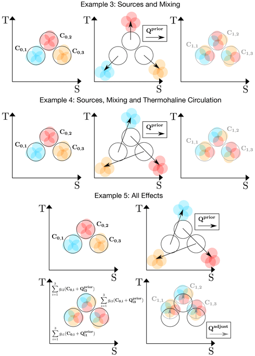
The toy examples below are illustrated in Figs. 1 (for examples 1 and 2) and 2 (for examples 3, 4 and 5).

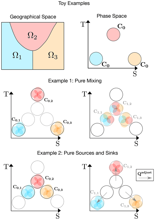
Figure 1 Illustration of the method using toy examples with three early (C_0,i) and three late (C_1,j) water masses in T–S coordinates. The water masses occupy geographical regions given by Ω_0,i. The fraction of the ith early water mass that arrives in the jth late water masses (g_ij) is represented by the coloured circles, each representing one-fourth of the water mass it came from and $\mathrm{1}/\mathrm{12}$ of the total mass in the system. For example, in the pure mixing example, two blue circles from early water mass 1 (i.e. half of water mass 1) arrive in late water mass 1, so that g₁₁=0.5, while one blue circle from early water mass 1 arrives at late water mass 2, so that g₁₂=0.25. Movements in the T–S space induced by sources and sinks are shown as arrows (black: priors, ${\mathit{Q}}_{ij}^{\mathrm{prior}}$; grey: adjustments, ${\mathit{Q}}_{ij}^{\mathrm{adjust}}$).

Figure 2 As in Fig. 1 but for the remaining toy examples.

2.7.1 Example 1: pure mixing

When there is no prior information given regarding the sources and sinks of tracers (${\mathit{Q}}_{ij}^{\mathrm{prior}}=\mathrm{0}$), optimisation of the inverse problem is achieved first by mixing water masses together, and then an adjustment is applied to complete the picture.

Three water masses form a triangle in the T–S space, initially with ${\mathit{C}}_{\mathrm{0},\mathrm{1}}=[\mathrm{0},\mathrm{34.6}]$, ${\mathit{C}}_{\mathrm{0},\mathrm{2}}=[\mathrm{4},\mathrm{35}]$ and ${\mathit{C}}_{\mathrm{0},\mathrm{3}}=[\mathrm{0},\mathrm{35.4}]$ and, at a later time, with ${\mathit{C}}_{\mathrm{1},\mathrm{1}}=[\mathrm{1},\mathrm{34.9}]$, ${\mathit{C}}_{\mathrm{1},\mathrm{2}}=[\mathrm{2},\mathrm{35}]$ and ${\mathit{C}}_{\mathrm{1},\mathrm{3}}=[\mathrm{1},\mathrm{35.1}]$. In this case the triangle contracts over time to form a smaller triangle. Equations (4) and (2) are satisfied for Q_ij=0, with g_ij=0.5 when i=j and g_ij=0.25 otherwise. Here the triangle is contracted by mixing the water masses together.

2.7.2 Example 2: pure sources and sinks

Now consider the case where ${\mathit{C}}_{\mathrm{0},\mathrm{1}}=[\mathrm{1},\mathrm{34.9}]$, ${\mathit{C}}_{\mathrm{0},\mathrm{2}}=[\mathrm{2},\mathrm{35}]$, ${\mathit{C}}_{\mathrm{0},\mathrm{3}}=[\mathrm{1},\mathrm{35.1}]$, ${\mathit{C}}_{\mathrm{1},\mathrm{1}}=[\mathrm{0},\mathrm{34.6}]$, ${\mathit{C}}_{\mathrm{1},\mathrm{2}}=[\mathrm{4},\mathrm{35}]$ and ${\mathit{C}}_{\mathrm{1},\mathrm{3}}=[\mathrm{0},\mathrm{35.4}]$. Here, the triangle expands. Intuitively this cannot be achieved by mixing, which is a convergent process in the T–S space. Indeed, Eq. (4) could be satisfied with Q_ij=0 but only by violating Eq. (2) (effectively, the water masses would need to be “unmixed”). With ${\mathit{Q}}_{ij}^{\mathrm{prior}}=\mathrm{0}$, a minimum cost (Eq. 6) is found with g_ij=1 when i=j and g_ij=0 otherwise. So, the change in water masses is achieved not by mixing the water masses, but instead by translating the corners of the triangle outward via adjustment to the sources and sinks (${\sum }_{i=\mathrm{1}}^N{g}_{ij}{\mathit{Q}}_{ij}^{\mathrm{adjust}}$).

2.7.3 Example 3: sources and mixing

Now consider an example where the three initial water masses do not change between the early and late periods with ${\mathit{C}}_{\mathrm{0},\mathrm{1}}=[\mathrm{1},\mathrm{34.9}]={\mathit{C}}_{\mathrm{1},\mathrm{1}}$, ${\mathit{C}}_{\mathrm{0},\mathrm{2}}=[\mathrm{2},\mathrm{35}]={\mathit{C}}_{\mathrm{1},\mathrm{2}}$ and ${\mathit{C}}_{\mathrm{0},\mathrm{3}}=[\mathrm{1},\mathrm{35.1}]={\mathit{C}}_{\mathrm{1},\mathrm{3}}$. In this case the triangle appears not to move. Now consider prior sources or sinks such that ${\mathit{C}}_{\mathrm{0},\mathrm{1}}+{\mathit{Q}}_{\mathrm{1}j}^{\mathrm{prior}}=[\mathrm{0},\mathrm{34.6}]$, ${\mathit{C}}_{\mathrm{0},\mathrm{2}}+{\mathit{Q}}_{\mathrm{2}j}^{\mathrm{prior}}=[\mathrm{4},\mathrm{35}]$ and ${\mathit{C}}_{\mathrm{0},\mathrm{3}}+{\mathit{Q}}_{\mathrm{3}j}^{\mathrm{prior}}=[\mathrm{0},\mathrm{35.4}]$ for all j. A solution then exists with no cost, according to Eq. (6). That is, a valid solution can be found with mixing alone. This occurs when g_ij=0.5 for i=j and g_ij=0.25 otherwise (as in the pure mixing case). In this solution, the sources and sinks expand the triangle and, according to the transport matrix, the water masses are then mixed together, contracting the triangle to achieve an unchanged water mass distribution.

2.7.4 Example 4: sources, mixing and thermohaline circulation

Consider once again a situation where the three initial water masses are the same for the early and late periods with ${\mathit{C}}_{\mathrm{0},\mathrm{1}}=[\mathrm{1},\mathrm{34.9}]$, ${\mathit{C}}_{\mathrm{0},\mathrm{2}}=[\mathrm{2},\mathrm{35}]$ and ${\mathit{C}}_{\mathrm{0},\mathrm{3}}=[\mathrm{1},\mathrm{35.1}]$ as well as ${\mathit{C}}_{\mathrm{1},\mathrm{1}}=[\mathrm{1},\mathrm{34.9}]$, ${\mathit{C}}_{\mathrm{1},\mathrm{2}}=[\mathrm{2},\mathrm{35}]$ and ${\mathit{C}}_{\mathrm{1},\mathrm{3}}=[\mathrm{1},\mathrm{35.1}]$. Now consider a prior source or sink such that ${\mathit{C}}_{\mathrm{0},\mathrm{1}}+{\mathit{Q}}_{\mathrm{1}j}^{\mathrm{prior}}=[\mathrm{0},\mathrm{35.4}]$, ${\mathit{C}}_{\mathrm{0},\mathrm{2}}+{\mathit{Q}}_{\mathrm{2}j}^{\mathrm{prior}}=[\mathrm{0},\mathrm{34.6}]$ and ${\mathit{C}}_{\mathrm{0},\mathrm{3}}+{\mathit{Q}}_{\mathrm{3}j}^{\mathrm{prior}}=[\mathrm{4},\mathrm{35}]$ for all j. Again, a solution exists with no cost (Eq. 6). However, rather than a symmetric matrix, we have g₁₂=0.5, g₂₃=0.5, g₃₁=0.5 and g_ij=0.25. Here, the transport matrix describes both mixing and clockwise circulation of the water masses in the T–S space. The latter circulation aspect is represented by the anti-symmetric part of the transport matrix. If the water masses are associated with fixed geographical regions, the anti-symmetric part of the transport matrix represents the thermohaline component of the geographical circulation (Zika et al., 2012).

2.7.5 Example 5: all effects

Finally, consider the case where the water masses change in time with ${\mathit{C}}_{\mathrm{0},\mathrm{1}}=[\mathrm{1},\mathrm{34.9}]$, ${\mathit{C}}_{\mathrm{0},\mathrm{2}}=[\mathrm{2},\mathrm{35}]$ and ${\mathit{C}}_{\mathrm{0},\mathrm{3}}=[\mathrm{1},\mathrm{35.1}]$ as well as ${\mathit{C}}_{\mathrm{1},\mathrm{1}}=[\mathrm{2},\mathrm{34.9}]$, ${\mathit{C}}_{\mathrm{1},\mathrm{2}}=[\mathrm{3},\mathrm{35}]$ and ${\mathit{C}}_{\mathrm{1},\mathrm{3}}=[\mathrm{2},\mathrm{35.1}]$. Let us assume prior sources or sinks that describe a steady source–mixing cycle as in the previous example but do not capture the overall warming, i.e. ${\mathit{C}}_{\mathrm{0},\mathrm{1}}+{\mathit{Q}}_{\mathrm{1}j}^{\mathrm{prior}}=[\mathrm{0},\mathrm{35.4}]$, ${\mathit{C}}_{\mathrm{0},\mathrm{2}}+{\mathit{Q}}_{\mathrm{2}j}^{\mathrm{prior}}=[\mathrm{0},\mathrm{34.6}]$ and ${\mathit{C}}_{\mathrm{0},\mathrm{3}}+{\mathit{Q}}_{\mathrm{3}j}^{\mathrm{prior}}=[\mathrm{4},\mathrm{35}]$ for all j. In this case no solution exists without a cost (Eq. 6). With the weights constant, the lowest cost is achieved by the same transport matrix as in the source, mixing and circulation example, with g₁₂=0.5, g₂₃=0.5, g₃₁=0.5 and g_ij=0.25. The remaining adjustment to each water mass (${\mathit{Q}}_{ij}^{\mathrm{adjust}}$) is then simply [0,1] for all i and j. That is, the sources and sinks will satisfy Eq. (4) if 1 °C of warming is added to each water mass. In this example, different weights could lead to differing distributions of the warming across the water masses and consequent changes in the transport matrix.

2.8 Summary of the optimal transformation method

In this section we have outlined a water-mass-based state estimation framework, the optimal transformation method. OTM relates knowledge of changing ocean tracer distributions to transient ocean transport and mixing. We propose an inverse method based on this framework to infer minimal adjustments to prior estimates of tracer sources and sinks.

In the following sections we will discuss one practical implementation of OTM and assess it using data from a historical climate model simulation.

3 Data and implementation

3.1 Synthetic data from a historical climate simulation

In Sect. 2, a general implementation of OTM was presented for any set of tracers. In this work, we demonstrate an implementation of this framework by analysing changes in temperature and salinity (and their associated surface fluxes of heat and freshwater) in a climate model.

We analyse ocean conservative temperature (hereafter temperature or T) and ocean practical salinity (hereafter salinity or S) from a historical simulation of the Australian Community Climate and Earth System Simulator - Climate Model version 2 (ACCESS-CM2) climate model, which forms part of the Australian submission to the Climate Model Intercomparison Project Phase 6 (CMIP6). The Modular Ocean Model (MOM, version 5.1) is used as the ocean component of the coupled ACCESS-CM2 model. We analyse the three-dimensional, monthly averaged conservative temperature and practical salinity field from January 1979 to December 2014 (inclusive) in ACCESS-CM2. Surface fluxes Q_i are obtained from the surface heat and freshwater flux variables (hfds and wfo), except in Sect. 4.3, where a reanalysis product is used instead (see below). Surface flux tendencies are obtained by time-integrating the relevant flux variables over the period of interest and then taking a time derivative over this period, following Sohail et al. (2021, 2022). The early period covers the time from January 1979 to December 1987, and the late period covers the time from January 2006 to December 2014.

Temperature and salinity exhibit a long-term climate drift in ACCESS-CM2 (further explored by Irving et al., 2020). Despite this long-term drift, the heat and freshwater budgets close in the model (that is, the globally integrated cumulative surface flux is equal to the ocean heat and freshwater content change). Provided the heat and freshwater budgets close, the long-term drift in the ACCESS-CM2 model is immaterial for the purposes of validating the OTM state estimation framework laid out in Sect. 2. Thus, we analyse the drifting historical simulation in this work. Further details on the model spin-up, forcing and drift are provided by Bi et al. (2020), Mackallah et al. (2022) and Irving et al. (2020).

To test the performance of the OTM algorithm in a spatially heterogeneous bias, in Sect. 4.3 we apply known air–sea fluxes, ${\mathit{Q}}_{ij}^{\mathrm{prior}}$, from an air–sea reanalysis product, ERA5 (Hersbach et al., 2020). Produced by the European Centre for Medium-Range Weather Forecasts (ECMWF), ERA5 combines a wide range of atmospheric and oceanic observational products with an operational weather forecasting model (the Integrated Forecasting System (IFS), Cy41r2) using 4D-Var data assimilation. The result is a well-constrained, long-term representation of our best estimate of known air–sea fluxes. We assess the two-dimensional, gridded monthly averaged net surface heat and freshwater fluxes in ERA5 from January 1979 to December 2014. The ERA5 surface flux fields are re-binned onto the ACCESS-CM2 native grid prior to assessment with OTM to ensure that the ERA5 global net surface fluxes are captured accurately in the analysis.

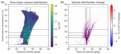
Figure 3 (a) The global distribution of ocean volume in the T–S space, averaged between January 1979 and December 2014, in the historical simulation of the ACCESS-CM2 climate model. (b) Volume distribution change between the time-averaged “early” and “late” periods, defined as January 1979–December 1987 and January 2006–December 2014, respectively. Black boxes show the 16 bins defined using binary space partitioning, each of which contains $\mathrm{1}/\mathrm{16}$ of the volume of the upper 2000 m of the ocean (since these data come from a Boussinesq ocean model, mass and volume are proportional).

3.2 Definition of discrete water masses using binary space partitioning

The global ocean's temperature–salinity (T–S) distribution is an integrated measure of its hydrographic properties, displaying the volume or mass of the ocean with a characteristic temperature and salinity range (Fig. 3).

Our OTM state estimation framework considers the transformation from a set of early water masses to a set of late water masses in tracer and geographical space. We split the ocean into nine basins (following Zika et al., 2021): the polar North Atlantic, sub-tropical North Atlantic, equatorial Atlantic, South Atlantic, Indian, South Pacific, equatorial Pacific, North Pacific and Southern. Only transport between adjacent ocean basins is permitted in the optimisation problem, such that g_ij=0 between water masses in non-adjacent basins. Ideally, the discrete representation should be as fine as possible so as to best describe our T–S distribution (i.e. as many discrete water masses as possible) while also considering the distributions that are representative of different geographical regions. However, computational constraints limit the resolution and number of regions that are possible. Here, we define the discrete water masses using binary space partitioning (BSP), following Sohail et al. (2023).

The BSP algorithm recursively sub-divides the mass-weighted T–S distributions along the T and S axes n times, resulting in 2ⁿ bins which all contain exactly the same mass. BSP represents an improvement over the quadtree coarsening algorithm (as used by Zika et al., 2021) as it results in a pre-determined number of bins which hold exactly the same volume. Note that the BSP coarsening presented here is a two-dimensional equivalent of the one-dimensional tracer–percentile framework introduced by Sohail et al. (2021, 2022). Further information on binary space partitioning and its applications in oceanography is provided in Sohail et al. (2023).

3.3 Implementation of the inverse model

We recursively sub-divide the T–S distribution of the top 2000 m of the global ocean in ACCESS-CM2 four times to yield 2⁴=16 classifications of equal volume or mass globally (since ACCESS-CM2's ocean component is Boussinesq, volume and mass are proportional to one another). We further partition these 16 T–S classifications into each of the nine basins defined above over the full ocean depth. This produces what we define as our 144 early and 144 late water masses. Each water mass has different tracer concentrations (${\mathit{C}}_{\mathrm{0},i}=[T_{\mathrm{0},i},S_{\mathrm{0},i}]$ and ${\mathit{C}}_{\mathrm{1},j}=[T_{\mathrm{1},j},S_{\mathrm{1},j}]$) and, due to the splitting by region, different masses (m_1,i and m_0,i). Figure 4 shows the mean temperature and salinity of each of these water masses (white dots), together with the volume (colour) and T–S ranges (rectangles) in each basin.

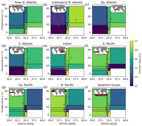
Figure 4 Volume (colours) and mean T and S of each of the 16 bins in each of the nine basins analysed in the early period. Each rectangle represents the range of T–S values covered by one of the water masses. The colour of the rectangle represents the volume of water in that bin in that basin. Each white point contained within a rectangle is located at the average T–S value of the water in that bin in that basin.

Each water mass has a corresponding “mask”, with ${\mathrm{\Omega }}_i(x,y,z,t)$ defining its geographical location with time (Ω_i=1 within the water mass and Ω_i=0 outside; x, y and z are latitude, longitude and depth, respectively). The outcrop area of water mass i at time t is then $\iint {\mathrm{\Omega }}_i(x,y,\mathrm{0},t)dA$, and A_i is the time average of that area (defined below).

The following hard constraints are placed on the entries of the transport matrix g_ij (note that the variable early and late masses m_0,i and m_1,i have been incorporated into the constraints below):

$$\begin{array}{}\text{(8)}& {\displaystyle }\mathrm{0}\le g_{ij}\le \mathrm{1};\text{(9)}& {\displaystyle }{m}_{\mathrm{1},j}=\sum _{i=\mathrm{1}}^N{m}_{\mathrm{0},i}{g}_{ij};\text{(10)}& {\displaystyle }{m}_{\mathrm{0},i}=\sum _{j=\mathrm{1}}^N{m}_{\mathrm{1},j}{g}_{ij};\text{(11)}& {\displaystyle }{\mathit{C}}_{\mathrm{1},j}{m}_{\mathrm{1},j}=\sum _{i=\mathrm{1}}^N{\mathit{C}}_{\mathrm{0},i}{m}_{\mathrm{0},i}{g}_{ij},\text{ where }{A}_j=\mathrm{0};\text{(12)}& {\displaystyle }{g}_{ij}=\mathrm{0}\text{ if }{\mathrm{\Omega }}_i\text{ and }{\mathrm{\Omega }}_j\text{ are not in the same or adjacent regions.}\end{array}$$

The above enforce mass conservation (Eqs. 8–10), tracer conservation away from the surface boundary (Eq. 11) and the inability of water to move further than the adjacent basin (Eq. 12).

A transport matrix g_ij is then sought which minimises the following cost function:

$$\begin{array}{}\text{(13)}& \mathrm{\text{[cost]}}=\sum _{j=\mathrm{1}}^N{\left|\left|{\mathit{w}}_j\left(\sum _{i=\mathrm{1}}^N{m}_{\mathrm{0},i}{g}_{ij}\left({\mathit{C}}_{\mathrm{0},i}+{\mathit{Q}}_{ij}^{\mathrm{prior}}\right)-m_{\mathrm{1},j}{\mathit{C}}_{\mathrm{1},j}\right)\right|\right|}^{\mathrm{2}},\end{array}$$

with

$$\begin{array}{}\text{(14)}& {\mathit{w}}_j={\displaystyle \frac{\mathrm{1}}{A_j}}\left[{\displaystyle \frac{\mathrm{1}}{\text{SD}\left(T\right)}},{\displaystyle \frac{\mathrm{1}}{\text{SD}\left(S\right)}}\right].\end{array}$$

Effectively, w_j leads Eq. (13) to search for the smallest residual source or sink per unit outcrop area and normalises the impact of temperature and salinity on the residuals relative to their global standard deviations. The additional constraint on g_ij (Eq. 11) ensures that changes to water masses that do not outcrop are achieved purely by redistribution and mixing. In one of the cases we will discuss below (where ${\mathit{Q}}_i^{\mathrm{prior}}=\mathrm{0}$), our optimiser does not find a feasible solution with this constraint when A_i=0 for some i values. In that case, we set a floor on those areas as the minimum non-zero A_j found for all j. This was, in that specific case, the most permissive area constraint we could justify for the problem.

We set the prior change in the tracer concentration driven by tracer sources and sinks to the same value for all early water masses i regardless of their path to the late water masses j (so ${\mathit{Q}}_{ij}^{\mathrm{prior}}$ becomes ${\mathit{Q}}_i^{\mathrm{prior}}$). We calculate this by integrating the known model air–sea fluxes over the outcrop region of the early water mass and over the time interval between the early and late periods such that

$$\begin{array}{}\text{(15)}& {\mathit{Q}}_i^{\mathrm{prior}}={\displaystyle \frac{\mathrm{1}}{m_{\mathrm{0},i}(t_{\mathrm{1}}-t_{\mathrm{0}})}}\underset{t_{\mathrm{0}}}{\overset{t_{\mathrm{1}}}{\int }}\iint {\mathrm{\Omega }}_i(x,y,\mathrm{0},t)\mathbf{q}(x,y,t)\mathrm{d}x\mathrm{d}y\mathrm{d}t,\end{array}$$

where t₀ and t₁ are the midpoints of the early and late periods. Above, $\mathbf{q}(x,y,t)=\left[\text{hfds}\right(x,y,t),-S_{\mathrm{0}}\text{wfo}(x,y,t\left)\right]+\text{bias}$, where “bias” is a bias we will introduce in some cases to see what effect incorrect air–sea flux data have on the inverse solution. The above time integral is from the midpoint of the early period to the midpoint of the late period since it is related to the change in average water mass properties between the two periods. (Integrating from the start of the early period to the end of the late period would overestimate the sources and sinks.)

In our implementation of the optimisation (Eq. 13), we aim to minimise the average adjustment to the tracer sources and sinks in a per unit area sense. For this reason we calculate the average outcrop area using the same integral limits as the sources and sinks such that

$$\begin{array}{}\text{(16)}& A_i={\displaystyle \frac{\mathrm{1}}{t_{\mathrm{1}}-t_{\mathrm{0}}}}\underset{t_{\mathrm{0}}}{\overset{t_{\mathrm{1}}}{\int }}\iint {\mathrm{\Omega }}_i(x,y,\mathrm{0},t)\mathrm{d}x\mathrm{d}y\mathrm{d}t.\end{array}$$

Equations (8) to (13) define a conic linear optimisation problem. We solve this numerically with the Python-based cvxpy package, specifying the “MOSEK” optimisation solver with default settings to obtain a transport matrix g_ij which satisfies the constraints described over the time period of interest.

4 Results

When a solution for g_ij is found by minimising Eq. (13), an adjustment to the tracer sources and sinks is implied in order to close the tracer budgets. We diagnose this adjustment via

$$\begin{array}{}\text{(17)}& {\mathit{Q}}_j^{\mathrm{adjust}}={\mathit{C}}_{\mathrm{1},j}-{\displaystyle \frac{\mathrm{1}}{m_{\mathrm{1},j}}}\sum _{i=\mathrm{1}}^N{m}_{\mathrm{0},i}{g}_{ij}\left({\mathit{C}}_{\mathrm{0},i}+{\mathit{Q}}_i^{\mathrm{prior}}\right).\end{array}$$

Once the early water masses have been redistributed and mixed by g_ij, ${\mathit{Q}}_j^{\mathrm{adjust}}$ is the remaining change in tracer concentrations required for these mixtures to match the late water mass concentrations, C_1,j. We do not attribute different adjustments to the different fractions of the early water masses that make up the late water masses, so that ${\mathit{Q}}_j^{\mathrm{adjust}}$ is the same for all i.

The inverse solution describing the evolution of ocean water masses is then the transport matrix g_ij and the implied total sources and sinks of the tracer given by Q^prior+Q^adjust. Since, in the case of heat and salt, we attribute the sources and sinks to fluxes at the sea surface, the adjustment term is converted into a flux per unit area and is mapped onto geographical coordinates via

$$\begin{array}{}\text{(18)}& {\mathbf{q}}_{\mathrm{adjust}}(x,y,t)=\sum _{j=\mathrm{1}}^N{\displaystyle \frac{m_j}{A_j(t_{\mathrm{1}}-t_{\mathrm{0}})}}{\mathit{Q}}_j^{\mathrm{adjust}}{\mathrm{\Omega }}_j(x,y,\mathrm{0},t).\end{array}$$

Above, the tracer source required to change water mass j by ${\mathit{Q}}_j^{\mathrm{adjust}}$ is applied as a flux of tracer per unit area. Because we only infer one adjustment flux per water mass, we are not able to infer more detailed variations in the flux over the spatial extent of the water mass outcrop.

The known surface fluxes, ${\mathit{Q}}_i^{\mathrm{prior}}$, are mapped onto the finite water masses obtained from the BSP coarsening (see Fig. 5). As the outcrop area of the water masses is much larger than the original model grid, the resulting remapped surface fluxes are smoother than the raw fields, as shown in Fig. 5.

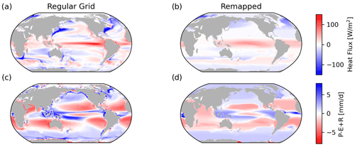
Figure 5 Time-averaged surface fluxes between the early and late periods in ACCESS-CM2, in the original model grid ($\mathbf{q}(x,y,t)$; a and c) and remapped onto the 2ⁿ×9 water masses as defined by BSP in the T–S space (${\mathit{Q}}_i^{\mathrm{prior}}$; b and d). Note that the surface outcrop location of these water masses, averaged over the entire early period, is used for the remapping.

In the remainder of this section we will discuss three applications of the inverse method with the same tracer data but different priors for the tracer sources and sinks. Case 1 shows the “true” tracer sources and sinks from the numerical model, Case 2 shows the true numerical model sources and sinks with a bias added globally, and Case 3 shows the prior sources and sinks set to zero globally.

4.1 Case 1: true source and sink priors

When the true model fluxes are used for Q^prior (bias=0), the inverse method is able to find a solution for g_ij which matches these priors with little Q^adjust necessary (Fig. 6). Quantitatively, the standard deviation of the true fluxes (SD(q_prior); the signal) is [17.6 W m⁻², 1.57 mm d⁻¹], while the standard deviation of the adjustment (SD(q_adjust); the error) is [$\mathrm{9.6}\times {\mathrm{10}}^{-\mathrm{3}}$ W m⁻², $\mathrm{7.4}\times {\mathrm{10}}^{-\mathrm{5}}$ mm d⁻¹], yielding a signal-to-error ratio of, at minimum, order 2000.

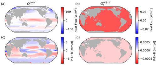
Figure 6 Case 1: time-averaged surface fluxes between the early and late periods in ACCESS-CM2, remapped onto the 16×9 water masses as defined by BSP in the T–S space (${\mathit{Q}}_i^{\mathrm{prior}}$; a and c), and the inferred surface flux adjustment based on changes to the underlying ocean T–S distribution (${\mathit{Q}}_j^{\mathrm{adjust}}$; b and d). Note that the surface outcrop location of the water masses, averaged over the entire early period, is used for the remapping. Note the differences in the colour bar ranges between panels (a) and (c) and panels (b) and (d).

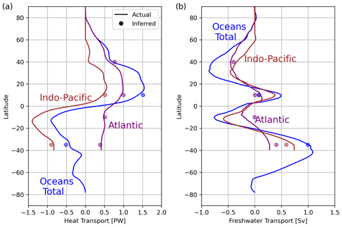
From the inferred transport matrix g_ij, the region-to-region heat and freshwater transport is determined using

$$\begin{array}{}\text{(19)}& {\displaystyle }\text{[heat transport]}=C_p{\mathit{\rho }}_{\mathrm{0}}\sum _{i=\mathrm{1}}^N{m}_{\mathrm{0},i}(T_{\mathrm{0},i}+{\mathit{Q}}_i^{\mathrm{prior}})g_{ij}{\mathit{\delta }}_{ij},\text{(20)}& {\displaystyle }\begin{array}{rl}& \text{[freshwater transport]}=-{\mathit{\rho }}_{\mathrm{0}}/S_{\mathrm{0}}\sum _{i=\mathrm{1}}^N{m}_{\mathrm{0},i}\\ & \cdot (S_{\mathrm{0},i}+{\mathit{Q}}_i^{\mathrm{prior}})g_{ij}{\mathit{\delta }}_{ij},\end{array}\end{array}$$

where C_p is the heat capacity of seawater (3992.1 J kg⁻¹ K⁻¹), ρ₀ is a reference density (1035 kg m⁻³), and S₀ is a reference salinity (35 g kg⁻¹). Above, δ_ij=1 if the flow from i to j implies “positive” transport across a region-to-region boundary (e.g. northward across a zonal section), ${\mathit{\delta }}_{ij}=-\mathrm{1}$ if the flow from i to j implies “negative” transport (e.g. southward), and δ_ij=0 if water masses i and j are not in adjacent regions. We only consider region-to-region boundaries where the total mass transport is zero.

We compare the heat transport in ACCESS-CM2, inferred directly from the model output, to our inverse estimate (based on Eq. 19), and the two match to within standard deviations across the region-to-region boundaries of 17 TW in the Indo-Pacific region and 16 TW in the Atlantic. Comparing the explicitly calculated freshwater transport in ACCESS-CM2 to our inverse estimate, we find that the two match to within standard deviations of 0.14 Sv in the Indo-Pacific region and 0.014 Sv in the Atlantic (Fig. 7).

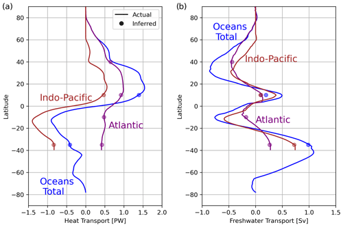
Figure 7 Case 1: meridional (a) heat transport and (b) freshwater transport inferred from the transport matrix g_ij (dots, located at the boundaries between adjacent regions) and from the surface fluxes and ocean heat or freshwater content change in the ACCESS-CM2 model (lines). We have omitted the same figure for Case 2 since the solution is indistinguishable.

It is reassuring that, when applied to consistent tracer source and tracer change data, an accurate solution is confirmed. We now consider what happens when the prior source estimates contain biases.

4.2 Case 2: spatially uniform biased source and sink priors

We add a constant offset to the air–sea fluxes of 5 W m⁻² for heat and 5 mm d⁻¹ for freshwater over the entire dataset (Fig. 8). We then use the biased air–sea fluxes to determine Q^prior and feed this into our inverse model. The inverse model finds a solution for g_ij and Q^adjust via Eq. (17), opposing the bias to within a standard deviation of $\mathrm{2.9}\times {\mathrm{10}}^{-\mathrm{3}}$ mm d⁻¹ and $\mathrm{5.1}\times {\mathrm{10}}^{-\mathrm{2}}$ W m⁻². The implied region-to-region heat transports of the inverse model with biased sources and sinks are virtually indistinguishable from the case without a bias, with a standard deviation that is within $\mathrm{1}\times {\mathrm{10}}^{-\mathrm{2}}$ of the values reported for Case 1 (Fig. 7).

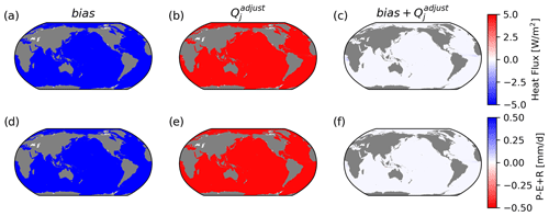
Figure 8 Case 2: constant offset added uniformly to ocean surface fluxes (bias; a and d), the inferred adjustment based on changes to the underlying ocean T–S distribution (${\mathit{Q}}_j^{\mathrm{adjust}}$; b and e) and the sum of the two (c, f). Note that the surface outcrop location of the water masses, averaged over the entire early period, is used for the remapping.

This suggests that the inverse model could be a useful tool for finding a consistent, and potentially more realistic, solution in the presence of biased estimates of air–sea fluxes.

We now consider how the inverse method adjusts the prior fluxes when a reanalysis flux field (ERA5) is imposed as a prior instead of the native model fluxes.

4.3 Case 3: air–sea reanalysis-based source and sink priors

Case 3 offers a more practical test than Cases 1 and 2 in that an incorrect yet plausible air–sea flux field is used as the prior. We use observational estimates of heat and freshwater fluxes (from ERA5; see Sect. 3) to determine Q^prior. We expect differences between these fluxes and the known model fluxes since the model is not a perfect representation of the real climate. This mimics a scenario where we have good knowledge of T and S changes, but air–sea fluxes have large biases which are heterogeneous. In this case, given that we know the true fluxes, we can see how well the inverse model does.

Figure 9 shows that ERA5 suggests warming across all ocean basins except for the Arctic relative to ACCESS and a heterogeneous pattern of freshwater flux change, particularly at middle to low latitudes, where rainfall is more intense on average.

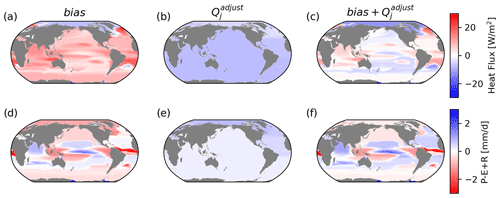
Figure 9 Case 3: the bias (a, d) is the difference between air–sea heat (a–c) and freshwater (d–f) fluxes in ERA5 and ACCESS. Panels (b) and (e) show the inferred adjustment using OTM, and panels (c) and (f) show the sum of the two. With the cost function in OTM minimising adjustments in a per unit area sense, this does not accurately correct the heterogeneous pattern of bias and favours a more spatially uniform adjustment.

The adjustment OTM findings in Case 3 are far more spatially homogeneous than the actual bias (Fig. 9b and e). This is likely due to our cost function weights, which penalise adjustments in a per unit area sense. That being said, some basin-scale patterns are captured well, with less (more) heat (freshwater) adjustment in the Arctic, for example, leading to accurate estimates of meridional transport between basins (Fig. 10).

Figure 10 As in Fig. 8 but for Case 3.

Finally, we consider what the inverse method yields when we ask it to estimate the sources and sinks with priors set to zero.

4.4 Case 4: zero source and sink priors

Cases 1 and 2 mirror toy examples 3 and 4 in Sect. 2. There, Q^prior effectively moved the water masses from their initial state to some intermediate state in tracer coordinates, and then g_ij moved them as close as possible to their final state, with Q^adjust providing the final adjustment. In our final case, we see how the inverse model responds to zero source or sink information, as in toy examples 1 and 2.

We run the inverse model, as in Cases 1 and 2, but for Q^prior=0. The Q^adjust patterns represent the smallest necessary heat and freshwater fluxes that can explain the model's water mass changes in conjunction with the redistribution and mixing achieved by g_ij. Since the model is describing historical climate change, increases in ocean heat content and any increase in the variance of ocean salinity cannot be described by g_ij and are captured in Q^adjust.

The resulting patterns of adjustments to the heat flux are approximately uniform across all the oceans, except for the polar regions (Fig. 11). In the inverse model solution, basin-scale anomalous warming–cooling patterns can be explained by redistribution via g_ij. Only a small, near-uniform warming is required to complete the picture. The patterns of adjustment to freshwater flux show net precipitation in relatively fresh regions of the globe, such as the tropical Pacific and sub-polar oceans, and net evaporation over relatively saline regions such as the sub-tropical oceans and the majority of the Atlantic basin. This is likely because greenhouse forcing in ACCESS-CM2 is consistent with the “wet gets wetter, dry gets drier” paradigm (Durack et al., 2012; Skliris et al., 2016), and the consequent changes in salinity cannot be affected by mixing, which can only make freshwater salty and salty water fresh (Zika et al., 2015b).

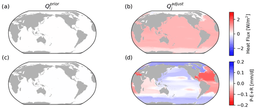
Figure 11 Case 4: surface flux adjustment given no prior source or sink information (${\mathit{Q}}_i^{\mathrm{prior}}=\mathrm{0}$; a and c) and the inferred surface flux adjustment based on changes to the underlying ocean T–S distribution (${\mathit{Q}}_j^{\mathrm{adjust}}$; b and d). Note that the surface outcrop location of the water masses, averaged over the entire early period, is used for the remapping.

The true air–sea fluxes warm the low latitudes and cool the high latitudes far more, and this is largely balanced by the heat transport and mixing represented by g_ij. Practically, a solution can always be added in which sources and sinks are balanced by the transport matrix while still satisfying our hard constraints (a “homogeneous solution” in the language of differential equations), but in the case where Q^prior=0, such additions are penalised since the inverse method searches for the solution with the smallest root mean squared error Q^adjust. These results suggest that, without adequate priors, the inverse method cannot by itself accurately determine the correct total tracer sources and sinks.

Figure 12 summarises the results of the four cases at the basin scale. It shows the net Q^prior (if any), Q^adjust, the divergence of tracer transport described by g_ij and the change in the amount of tracer with time in each region.

Case 1 describes the true budget for the time period considered with the change with time and a small residual of the larger source, sink and divergence terms. Case 2 shows how a small adjustment to the sources and sinks compensates for an imposed error.

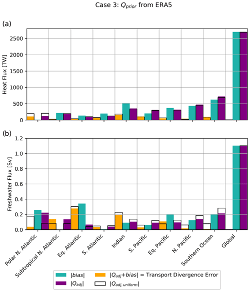
In Case 3 a spatially heterogeneous bias pattern is imposed. Despite the fact that the adjustment does not capture many of the finer geographical details, OTM does offer skill in balancing biases at the basin scale. Figure 13 shows a comparison of the magnitudes of the added bias and adjustment in response to Case 3.

In Case 4, the implied net Q and tracer transport divergence are 1 order of magnitude smaller than in Case 1 at the basin scale, since they are only required to describe the change rather than the large mean balances of sources or sinks and transport or mixing.

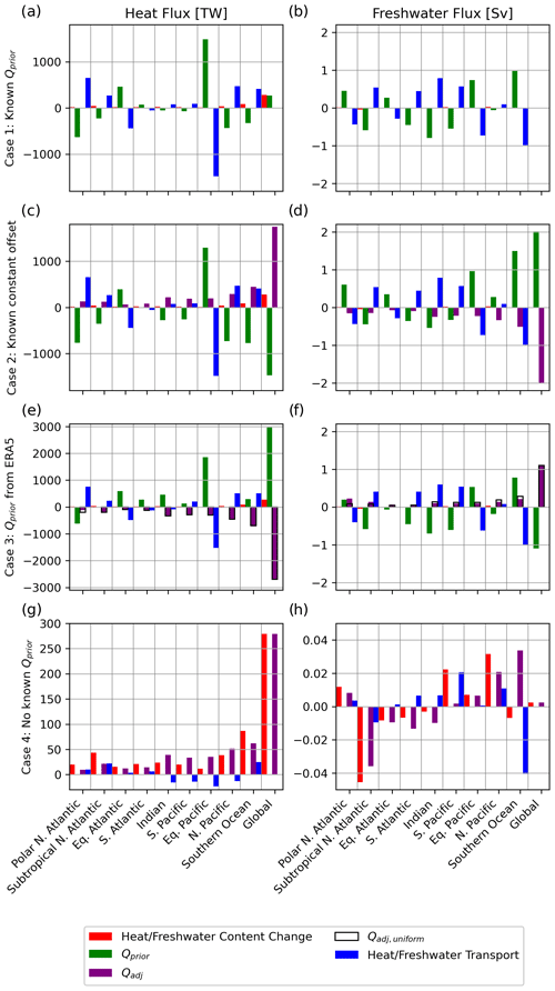
Figure 12 Terms in the heat and freshwater budgets for the four cases explored in this study. In this framework, heat or freshwater content change $={\mathit{Q}}_{\mathrm{adj}}+{\mathit{Q}}_{\mathrm{prior}}$ + heat or freshwater transport. For Case 1, the terms are indistinguishable from their true values in the ACCESS-CM2 model. For Case 3, unfilled bars show what the adjustment fluxes would be if they were globally spatially uniform.

Figure 13 Comparison of bias and adjustment heat (a) and freshwater (b) fluxes for Case 3. In Case 3, ERA5 fluxes are used instead of the models' true fluxes. Unfilled bars show what the adjustment fluxes would be if they were globally spatially uniform.

5 Discussion

Our assessment of the optimal transformation method state estimation framework has not been exhaustive. Our aim has been to describe the framework generally. In any future implementation, a number of choices can be made by the user, including the following:

1. the way in which water masses are defined in both space and time

2. the way in which constraints are placed on the transport matrix g_ij and priors are introduced

3. how adjustments of tracer sources or sinks and other variables impact the cost function.

For choice 1, we used binary space partitioning to objectively divide the tracer space into discrete water masses. However, we used conventional definitions of ocean basins to distinguish the water masses. OTM is not tied to either choice or alternative objective (e.g. machine-learning-based classification), and user-driven approaches (e.g. traditional water mass definitions) can be used. All that is required is that a set of water masses with tracer concentrations for two time periods (or a sequence of time periods) be defined and constraints placed on their connectivity (g_ij).

For choice 2, we chose to give no prior information about the transport matrix (g_ij). Priors for this matrix or stricter constraints on it could be given based on numerical models or observations at key regional boundaries (such as the Rapid Climate Change-Meridional Overturning Circulation and Heatflux Array: RAPID–MOCHA transect in the North Atlantic) and in key ocean gateways. Note, however, that g_ij does not necessarily represent the conventional transport measured at a section. To illustrate this, consider a water mass in the sub-tropical North Atlantic with temperature $T_{\mathrm{0},i}=\mathrm{20}$ °C that is heated due to some air–sea flux with an implied warming over a 40-year period of Q_i=80 °C. Let us assume that the state estimate tells us that 1 % of this water mass travels northward into the sub-polar North Atlantic and mixes with 99 % of the water contained in water mass j (i.e. g_ij=0.01 and g_jj=0.99). Mathematically, the water can be viewed as crossing the regional boundary at a temperature of $T_{\mathrm{0},i}+Q_i=\mathrm{100}$ °C, as used in the calculation for the heat transport (Eq. 19). A more plausible physical interpretation is that water from water mass j is continually mixing with water mass i. The state estimate does not describe where or when this mixing occurs, only that it occurred at some point between the early and late periods. Hence, further work is required to determine how information about the ocean overturning circulation can be used to constrain state estimates and likewise how the state estimate can inform us of the circulation.

For choice 3, in applications to observation-based data, choices should be guided by the uncertainty in the underlying data. For example, we minimised the sources and sinks in a per unit area sense. OTM broadly did a better job of assuming a completely homogeneous pattern of change (see for example the comparison between the unfilled and purple bars in Fig. 13) but did not accurately correct the biased pattern below the basin scale (Fig. 9). It could be that particular regions and/or components of the sources and sinks (e.g. precipitation) are more uncertain than others. These distinct uncertainties can be accounted for through the weight vector w_j.

An additional consideration that we have not explored here is the choice of spatial and temporal resolution. We chose to compare mid-20th century and early 21st century time periods and force these with fluxes integrated between their mid-point times. As the time period becomes longer, the fluxes can take the early water masses further and further apart in the phase space (e.g. extending the vectors in toy example 2). These more extreme water masses are easier for OTM to mix together (via g_ij) to form late water masses. In the most extreme case, air–sea fluxes would only be needed to translate the global centre of mass of the distribution into the tracer space, and g_ij could account for all spatial variation in the transformations. In that case, and in the absence of additional constraints on g_ij, OTM would have no skill in correcting spatial variations in tracer sources and sinks and would only correct the global mean.

6 Conclusions

We have presented a state estimation framework based on water mass theory, termed the optimal transformation method. The framework enables framing of inverse problems where ocean transport and tracer sources and sinks are optimally adjusted to define a self-consistent description of ocean change. We have used temperature and salinity data from a numerical climate model responding to historical natural and anthropogenic forcing over the past half-century to test one application of the framework.

The optimal transformation method draws on concepts in water mass transformation, water mass analysis and ocean tracer transport theory. What results is a set of equations describing how the ocean's multi-variate water mass distribution varies in time. These equations, combined with a transparent set of physically based constraints, allow for the definition of an inverse problem where a solution can be optimised based on deviations from priors.

We implemented an inverse method where the change in the ocean state was known, the ocean transport was unknown, and deviations from prior estimates of tracer sources and sinks were minimised. When given true heat and freshwater fluxes, the inverse solution found a state with near-zero deviation from those priors. Likewise, when given fluxes with a constant bias added, the method reduced the errors from 27.7 % to 1.0 % for heat flux and from 29.0 % to 1.1 % for freshwater flux. When given fluxes with spatially heterogeneous errors, the method did a better job of correcting for that error at the basin scale than a constant compensating offset.

The methods presented may be a useful complement to existing state estimation approaches, having the advantage of being relatively simple (for example when compared to numerical ocean models and ocean data assimilation platforms) and computationally cost-efficient. In particular, the optimal transformation method has shown promise for finding corrections to air–sea fluxes of heat and freshwater so that they plausibly describe the changing ocean state. This implies that the method, leveraged with observations, can help to refine observationally based estimates of the net heat and freshwater flux imbalance in the climate system.