Selecting CMIP6 global climate models (GCMs) for Coordinated Regional Climate Downscaling Experiment (CORDEX) dynamical downscaling over Southeast Asia using a standardised benchmarking framework

Downscaling global climate models (GCMs) provides crucial high-resolution data needed for informed decision-making at regional scales. However, there is no uniform approach to select the most suitable GCMs. Over Southeast Asia (SEA), observations are sparse and have large uncertainties, complicating GCM selection especially for rainfall. To guide this selection, we apply a standardised benchmarking framework to select CMIP6 GCMs for dynamical downscaling over SEA, addressing current observational limitations. This framework identifies fit-for-purpose models through a two-step process: (a) selecting models that meet minimum performance requirements in simulating the fundamental characteristics of rainfall (e.g. bias, spatial pattern, annual cycle and trend) and (b) selecting models from (a) to further assess whether key precipitation drivers (monsoon) and teleconnections from modes of variability are captured, i.e. the El Niño–Southern Oscillation (ENSO) and Indian Ocean Dipole (IOD). GCMs generally exhibit wet biases, particularly over the complex terrain of the Maritime Continent. Evaluations from the first step identify 19 out of 32 GCMs that meet our minimum performance expectations in simulating rainfall. These models also consistently capture atmospheric circulations and teleconnections with modes of variability over the region but overestimate their strength. Ultimately, we identify eight GCMs meeting our performance expectations. There are obvious, high-performing GCMs from allied modelling groups, highlighting the dependency of the subset of models identified from the framework. Therefore, further tests of model independence, data availability and future climate change spread are conducted, resulting in a final subset of two independent models that align with our a priori expectations for downscaling over the Coordinated Regional Climate Downscaling Experiment –Southeast Asia (CORDEX-SEA).

1 Introduction

The Sixth Assessment Report (AR6) of the Intergovernmental Panel on Climate Change (IPCC) underscores with high confidence the escalating water-related risks, losses and damage associated with each increment of global warming (IPCC, 2023). The report specifically notes a projected increase in the frequency and intensity of heavy rainfall, leading to an increased risk of rain-generated localised flooding, particularly in coastal and low-lying cities and regions (Sect. 3, IPCC, 2023). Therefore, climate projections at regional scales are required to inform climate change adaptation strategies and enhance resilience efforts.

Different types of models have been developed and have become fundamental tools for assessing future regional climate changes, including state-of-the-art global climate models (GCMs) and regional climate models (RCMs). GCMs are generally used to explore climate interactions and underpin climate projections through the Coupled Model Intercomparison Project (CMIP; Meehl et al., 2000), an initiative of the World Climate Research Programme (WCRP). However, with a typical horizontal resolution of 50–250 km, GCMs have limited ability to simulate sub-grid weather (e.g. local variance, persistence, topography, etc.) and therefore cannot accurately define local-scale processes and feedbacks (e.g. deep convection, land–atmosphere interactions, etc.). This limits GCMs' ability to simulate aspects of the present-day water cycle and to determine robust future changes for local and regional applications (Maraun and Widmann, 2018; Douville et al., 2021). RCMs dynamically downscale GCM outputs to create higher spatial resolutions of ∼ 2–50 km, providing richer regional spatial information (e.g. small-scale processes and extreme events) for climate assessments and for impact and adaptation studies (Diaconescu and Laprise, 2013; Giorgi and Gao, 2018). However, such experiments are computationally expensive, so it is not practical to choose all GCMs for dynamical downscaling. Thus, a subset of GCMs has to be selected.

The WCRP's Coordinated Regional Climate Downscaling Experiment (CORDEX) initiative delivers dynamically downscaled simulations of various GCMs (Giorgi and Gao, 2018) over 14 regions worldwide. This includes Phase I using CMIP5 (Giorgi et al., 2008) and Phase II, Coordinated Output for Regional Evaluations (CORDEX-CORE; Giorgi et al., 2021), as well as on-going experiments (CMIP6). However, there is no agreed upon approach to selecting which GCMs would be most suitable for dynamical downscaling, either in the recent WCRP guidelines for CMIP6 CORDEX experiments (CORDEX, 2021) or across different CORDEX domains (Di Virgilio et al., 2022; Grose et al., 2023; Sobolowski et al., 2023). In the earliest initiatives, GCMs were eliminated based on their skill at reproducing the current climate for the region of interest, given the fact that the bias in the GCMs can propagate into the RCM through the underlying and lateral boundary conditions (i.e. driven by initial and time-dependent meteorological variables from GCMs; Mote et al., 2011; Overland et al., 2011; McSweeney et al., 2012, 2015). In addition, the selection of GCMs considers the need to generate a reasonable uncertainty range for future climate projections (Mote et al., 2011; Overland et al., 2011). Given the shared physical components of the design of CMIP6 GCMs, there are inherent biases in statistical properties like the multi-model mean or standard deviation of the full ensemble (Boé, 2018; Brands, 2022; Sobolowski et al., 2023). To address this problem, model dependency is also considered. These considerations and methodologies have been integrated into the most recent CMIP6 CORDEX experimental design for specific regions, such as Europe (Sobolowski et al., 2023) or Australia (Di Virgilio et al., 2022) and are recommended for widespread application across other CORDEX domains.

Model evaluation is an essential part of CMIP6 model selection since simulating past performance well is a necessary (but insufficient) condition to have more confidence in future performance. Different metrics are employed to quantify model skill in simulating various climate variables at either global (Kim et al., 2020; Ridder et al., 2021; Wang et al., 2021b; Donat et al., 2023) or regional scales, e.g. in Australia (Deng et al., 2021; Di Virgilio et al., 2022), Europe (Ossó et al., 2023; Palmer et al., 2023), South America (Díaz et al., 2021), Asia (Dong and Dong, 2021) and Southeast Asia (Desmet and Ngo-Duc, 2022; Pimonsree et al., 2023). However, the lack of consistency in the list of metrics used makes it difficult to perform one-to-one comparisons between studies or to track model performance across various regions.

Recently, Isphording et al. (2024) introduced a standardised benchmarking framework (BMF) underpinned by the work of the US DOE (2020), which included a set of baseline performance metrics for assessing model performance in simulating different characteristics of rainfall. The BMF is different from traditional model evaluation in that it defines performance expectations a priori (Abramowitz, 2005, 2012; Best, 2015; Nearing et al., 2018). Under the BMF, a model will not be considered fit-for-purpose if it fails any performance metric. The BMF consists of two tiers of metrics: the first tier includes minimum standard performance metrics related to fundamental characteristics of rainfall, and the second tier allows users to define metrics that help to answer specific scientific research questions. The BMF was initially designed for rainfall but can be widely applied to other climate variables (e.g. surface temperature) depending on the user's purpose (Isphording et al., 2024).

IPCC highlights Southeast Asia (SEA) as a region facing considerable climate change risks from extreme events (e.g. floods, extreme heat, changing precipitation and extremes; IPCC, 2022). However, available regional climate simulations for SEA, particularly from CMIP5 CORDEX-SEA experiments are limited to 13 simulations (Tangang et al., 2020) compared to EURO-CORDEX with 68 simulations (Jacob et al., 2020) or CORDEX-Australasia with 20 simulations (Evans et al., 2021). Consequently, future projections come with a higher degree of uncertainty, especially for rainfall (Tangang et al., 2020; Nguyen et al., 2023). This motivated the CORDEX-SEA community to update their regional climate model simulations with the latest CMIP6 models. Note that over SEA, observations are sparse with large uncertainties, particularly for rainfall (Nguyen et al., 2020), making GCM evaluations more complicated (Nguyen et al., 2022; Nguyen et al., 2023). To date, the performance of various CMIP6 GCMs has been evaluated and ranked over the whole region of SEA (Desmet and Ngo-Duc, 2022; Pimonsree et al., 2023) and its sub-regions, e.g. the Philippines (Ignacio-Reardon and Luo, 2023), Thailand (Kamworapan et al., 2021) and Vietnam (Nguyen-Duy et al., 2023). Although there are groups of GCMs that consistently perform well (e.g. EC-Earth3, EC-Earth3-Veg, GFDL-ESM4, MPI-ESM1-2-HR, E3SM1-0 and CESM2) and poorly (e.g. FGOALS-g3, CanESM, NESM3 and IPSL-CM6A-LR) across the available literature, their ranking varies given inconsistencies in evaluation metrics and observational reference datasets. This creates challenges in conducting direct intercomparisons across the abovementioned studies. In addition, it is crucial to consider other important aspects discussed above (e.g. observational uncertainty, model dependency and future climate change spread) in identifying the list of reliable models over SEA.

In this research, we aim to apply the lessons learnt from CMIP6 selection over different CORDEX domains for SEA by assessing different aspects of models: model performance, model independence, data availability and future climate change spread. We apply the BMF to provide a consistent set of metrics for holistically evaluating model performance and to deal with large observational uncertainties over the region. Focusing on precipitation, where future projections are much more uncertain, the objectives of this research are twofold.

• We aim to evaluate the performance of CMIP6 GCMs in simulating the fundamental characteristics of precipitation, its drivers and teleconnection with modes of variability over SEA using a standardised benchmark framework and to identify a subset of models that meet our performance expectations.

• We aim to retain models that are relatively independent and are representative of the full range of possible projected change for finalising a subset of CMIP6 GCMs for dynamical downscaling over SEA using model independence tests and assessment of climate change response patterns.

The structure of the paper is as follows: Sect. 2 introduces the data and the benchmarking framework employed in this study. The results are presented in three subsections. Section 3.1 focuses on model assessment using the benchmarking framework, Sect. 3.2 examines the spread of future climate change among models and Sect. 3.3 assesses model dependence through cluster analysis. Finally, we conclude with a discussion of our results in Sect. 4 and a summary of the main conclusions in Sect. 5.

Table 1 Information on model components from the CMIP6 GCMs used in this study.

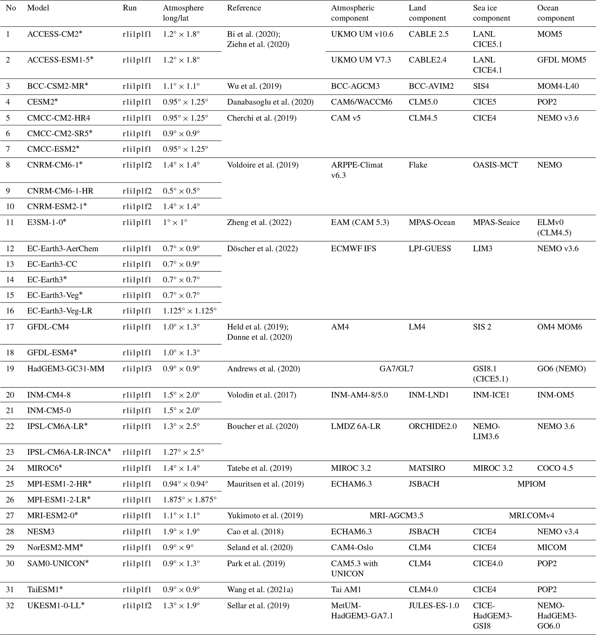
^* The model offers atmospheric variables available in three dimensions every 6 h for dynamical downscaling at the time of analyses.

2 Methods

2.1 Data

2.1.1 CMIP6 GCM data

We use the historical daily data of precipitation, near-surface temperature, 850 hPa wind speed and both monthly and daily sea-surface temperature data from the 32 CMIP6 models listed in Table 1. We consider only models that have a horizontal grid spacing finer than 2° × 2°, which are likely to be more suitable for dynamical downscaling. One simulation (typically the first member r1i1f1p1) is utilised in the benchmarking process to enable a fair comparison. At the time of this analysis, the first member of some models (e.g. the CNRM-family models, UKESM1-0-LL and HadGEM3-GC31-MM) was not available, so another member was utilised.

Table 2 The main characteristics of observational datasets used in this study.

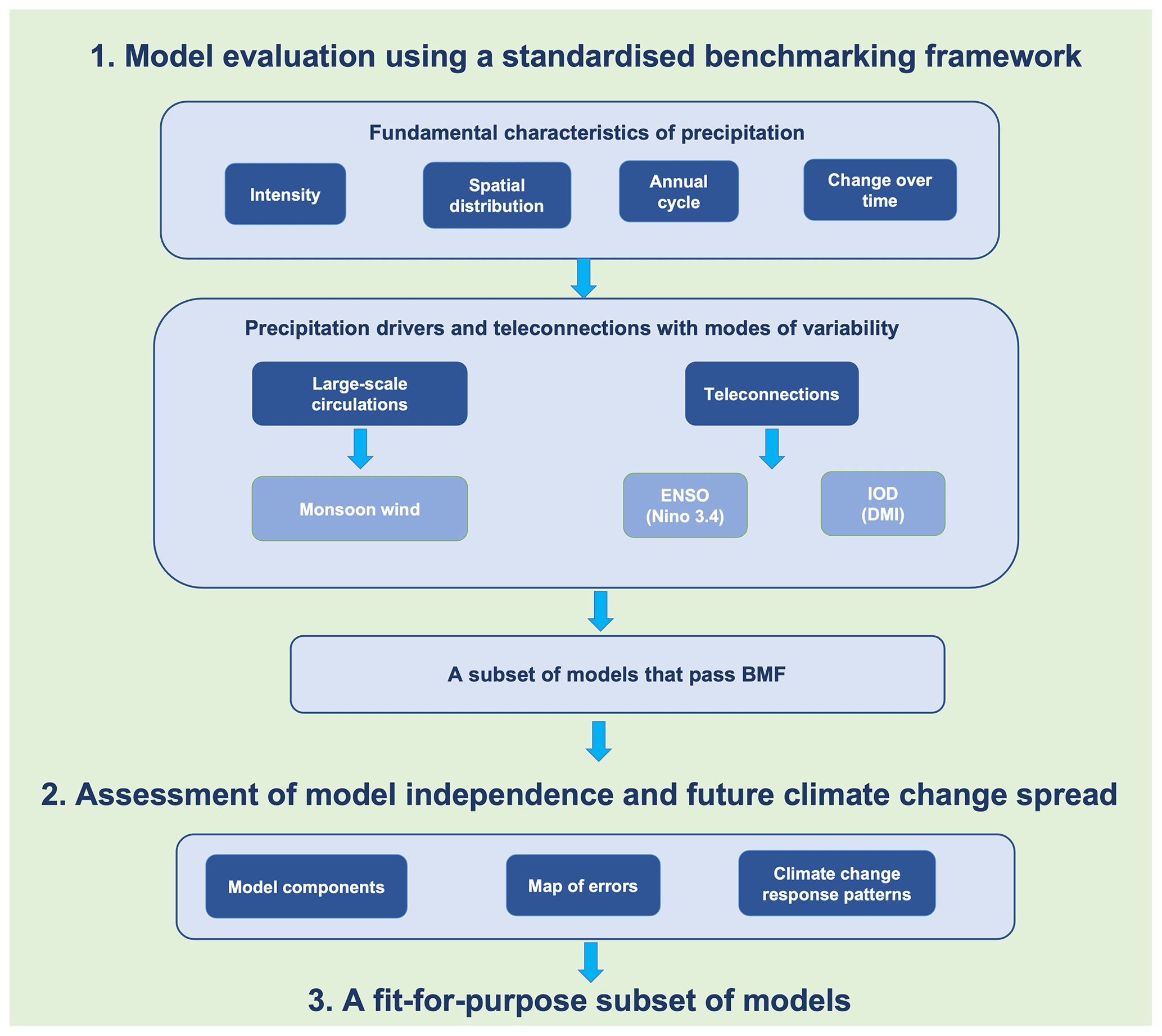
Figure 1 A schematic of the CMIP6 GCM selection process, including (1) model evaluation using a standardised benchmarking framework (BMF) and (2) assessment of model independence and future climate change spread. The BMF includes two steps: minimum standard metrics (MSMs) that assess very basic characteristics of rainfall and second-tier metrics (e.g. versatility metrics) that quantify the model skill of the models that pass the MSMs in simulating precipitation drivers (monsoon) and teleconnections with modes of variability, i.e. the El Niño–Southern Oscillation (ENSO) and Indian Ocean Dipole (IOD).

2.1.2 Observations and reanalyses

Given the large observational uncertainty in precipitation over the region (Nguyen et al., 2022), we use multiple daily observed datasets from different in situ and satellite sources to quantify model skill (Table 2). These datasets have been chosen given their high consistency in representing daily precipitation (Nguyen et al., 2022) and extremes (Alexander et al., 2020; Nguyen et al., 2020) over SEA.

The ERA5 reanalysis (∼ 31 km grid resolution; Hersbach et al., 2020) was used to benchmark model performance in representing the climatology of atmospheric circulation (e.g. metrics related to horizontal wind at 850 hPa level are described in Sect. 2.2).

We acknowledge that different observational sea-surface temperatures (SSTs) have different abilities to capture signals of the modes of variability. Therefore, we utilise multiple SST products (Table 2) to take account of the observational uncertainties in simulating the teleconnection between rainfall and the main modes of variability, including the El Niño–Southern Oscillation (ENSO) and Indian Ocean Dipole (IOD) as described in Sect. 2.2.

2.2 Benchmarking CMIP6 GCMs over Southeast Asia

Given the large uncertainties and model inconsistency in rainfall projections, our main aim is to identify a subset of CMIP6 GCMs that meet our a priori expectations. That is, as a minimum requirement, a model should simulate past rainfall statistics over SEA reasonably well using consistent criteria. Figure 1 illustrates the GCM selection process applied in this research based on a standardised benchmarking framework (Isphording et al., 2024). A subset of CMIP6 GCMs that meet our model performance expectations are identified through a two-step process: (a) selecting models that meet minimum performance requirements in simulating the fundamental characteristics of rainfall (Fig. 1) and (b) selecting models from (a) to further assess performance in simulating precipitation drivers (e.g. monsoon) and teleconnections with modes of variability (Fig. 1).

2.2.1 Minimum standard metrics

The BMF introduces a set of minimum-standard metrics (MSMs): (1) mean absolute percentage error (MAPE), (2) spatial correlation (Scor), (3) seasonal cycle (Scyc) and (4) significant changes (SigT) (Isphording et al., 2024) to assess the skill of climate models in simulating fundamental characteristics of precipitation (e.g. magnitude of biases, spatial distributions, annual cycles and temporal variability). Before exploring complex processes, a model should meet performance expectations for these MSMs. Therefore, we initially calculate the MSMs for precipitation. In addition, we acknowledge that models should produce adequate present-day simulations of other fundamental climate variables like near-surface temperature. Hence, we also apply the MSMs for near-surface temperature in the Supplement. Given the strong seasonality of precipitation in the region (Juneng et al., 2016), the analyses related to precipitation are conducted at a seasonal scale (e.g. the dry season from November–April – NDJFMA – and the wet season from May–October – MJJASO). Meanwhile, temperature analyses are conducted at the annual scale.

Note that in this research, we focus only on precipitation over land given the lack of in situ references over the ocean. Some satellite-derived products provide oceanic precipitation data, but most of their temporal coverage is not sufficiently long to use as a reference. In addition, the observational uncertainties among satellite clusters in estimating oceanic precipitation over SEA are quite substantial, with discrepancies reaching up to 4 mm d⁻¹ (Fig. S1 in the Supplement).

2.2.2 Versatility metrics

The MSMs provide statistical measurements that are not always correlated with future projections (Knutti et al., 2010), given that some models may simulate historical precipitation well for the wrong reasons. A further recommendation is therefore to also assess model performance based on key physical processes (Doe, 2020; Nguyen et al., 2023). This approach offers additional insights into the relative roles of model biases at simulating large-scale environments versus the limitations of model parameterisations in generating precipitation biases. Therefore, we define second-tier versatility metrics to assess the GCMs selected from Sect. 2.2.1 in simulating the complex precipitation-related processes, including drivers and teleconnections with modes of variability.

Monsoon circulation

SEA is situated within the Asian monsoon regime, where atmospheric circulation is modulated by two primary monsoon systems: the Indian monsoon characterised by westerlies from the Bay of Bengal into northern parts of SEA, including the mainland and northern Philippines (along 10° N) during the boreal summer (JJAS) and reversed in direction during the boreal winter (DJF), and the Australian monsoon, e.g. easterlies from Australia to the Maritime Continent (MC) and Papua New Guinea (Chang et al., 2005). These monsoon systems drive regional rainfall seasonality. Therefore, we focus on assessing model skill in simulating the intensity and direction of monsoon wind (e.g. 850 hPa wind) for JJAS and DJF. While wind speed is evaluated using the MAPE and Scor metrics similar to the MSMs for precipitation and temperature, wind direction is quantified using an equation from Desmet and Ngo-Duc (2022):

$$\text{MD}={\displaystyle \frac{{\sum }_i{u}_i\times \mathrm{|}{\mathit{\theta }}_i-{\mathit{\theta }}_{i,\text{ref}}{\mathrm{|}}_{[\mathrm{0},\mathrm{180}]}}{{\sum }_i{u}_i}},$$

where u_i refers to the simulated wind speed at the grid i and θ_i and θ_i,ref are the wind direction at grid i in the simulated and reference data, respectively. $\mathrm{|}{\mathit{\theta }}_i-{\mathit{\theta }}_{i,\text{ref}}{\mathrm{|}}_{[\mathrm{0},\mathrm{180}]}$ is the absolute value of the difference at the ith grid between directions of simulated and reference wind speed (e.g. ERA5). The MD metric allows us to quantify the agreement in wind direction between two datasets in which the impact of high wind speed is taken into account.

ENSO, IOD and teleconnections

Various parts of SEA are also affected by two prominent modes of variability: the El Niño–Southern Oscillation (ENSO; Haylock and McBride, 2001; Chang et al., 2005; Juneng and Tangang, 2005; Qian et al., 2013) and the Indian Ocean Dipole (IOD; Xu et al., 2021) via atmospheric teleconnections. In this research, the teleconnection is defined by the temporal correlation between precipitation anomalies at each grid point and the ENSO–IOD indices.

To track ENSO variability, the Niño3.4 index (5° S–5° N and 160° E–120° W) (Trenberth and Hoar, 1997; Shukla et al., 2011) derived for the 1951–2014 period as area-mean monthly SST anomalies with respect to a 1961–1990 climatology is used. For IOD, we use the dipole mode index (DMI; Saji et al., 1999; Meyers et al., 2007). DMI measures differences in monthly SST anomalies between those in the west equatorial Indian Ocean (10° S–10° N, 50–70° E) and those in the east (90–110° S, 10° S–0° N).

We use a 5-monthly average Niño3.4 and IOD index to remove seasonal cycles. The resulting monthly time series are detrended using a fourth-order polynomial fit to remove the possible influence of a long-term trend and to better preserve high-amplitude (< 10 years) variability (Braganza et al., 2003).

Since ENSO typically matures toward the end of the calendar year (Rasmusson and Wallace, 1983), we consider ENSO developing years as year (0) and use the DJF means to identify ENSO events. Over SEA, ENSO interacts with the monsoon cycle, and due to the varying monsoon onsets between the northern and southern parts of the region, its seasonal evolution differs across regions (Fig. S2). In particular, there is a lagged negative correlation between rainfall and ENSO over the Maritime Continent (MC) and the Philippines, which develops from May to June, strengthens during July–August and reaches its highest correlation during September–October of the developing year (year 0). On the other hand, this negative correlation becomes prominent over the northern parts during the subsequent boreal spring (from March to May of the year +1; Wang et al., 2020; Chen et al., 2023). The negative correlation indicates dry anomalies during El Niño and/or wet anomalies during La Niña. Therefore, in the context of this research, we examine the lead–lag Pearson correlation of the DJF Niño3.4 index in the developing year (year 0) with two different seasonal rainfall patterns: May–October (MJJASO) of the developing year (year 0) and March–May (MAM) of the following year (year +1).

Furthermore, considering the stronger influence of the IOD and its associated teleconnection during SON compared to other seasons (McKenna et al., 2020), we calculated the in-phase Pearson correlation coefficient between the detrended precipitation anomaly and DMI for the SON season. The statistical significance of the correlation coefficient is tested using the Student t test (alpha = 0.05). Note that IOD could exist as part of ENSO (Allan et al., 2001; Baquero-Bernal et al., 2002), and their coexistence could have strong impacts on rainfall variability over many parts of SEA (D'Arrigo and Wilson, 2008; Amirudin et al., 2020), which is not investigated in this study.

The previous literature has often focused on assessing the robustness of rainfall teleconnections (e.g. spatial patterns and amplitudes) across CMIP model ensembles. These assessments typically involve examining agreement in the sign of teleconnections such as through rainfall anomaly composites (Langenbrunner and Neelin, 2013) and regional average teleconnection strength over land (Perry et al., 2020) or a combination of both (Power and Delage, 2018) rather than evaluating the skill of an individual model. However, since rainfall teleconnections across SEA exhibit spatial and seasonal variability, the above metrics may be substantially influenced by internal variability. For high-level qualification, we employ spatial correlation and simplified metrics to assess whether there are significant correlations between teleconnections, as recommended by Liu et al. (2024). We assess the similarity in the number of grid points detecting significant signals between observed and modelled teleconnections using a set of three metrics: hit rate (HR), miss rate (MR) and false-alarm rate (FAR) as follows:

$$\begin{array}{}\text{(1)}& {\displaystyle }\mathrm{\text{HR}}={\displaystyle \frac{\text{Area\hspace{0.17em} with\hspace{0.17em} correct\hspace{0.17em} sign\hspace{0.17em} of\hspace{0.17em} significant\hspace{0.17em} correlation}}{\text{Area\hspace{0.17em} with\hspace{0.17em} significant\hspace{0.17em} correlation\hspace{0.17em} in\hspace{0.17em} OBS}}}\text{(2)}& {\displaystyle }\mathrm{\text{MR}}={\displaystyle \frac{\begin{array}{c}\text{Area\hspace{0.17em} with\hspace{0.17em} significant\hspace{0.17em} correlation\hspace{0.17em} in\hspace{0.17em} OBS\hspace{0.17em} but}\\ \text{with\hspace{0.17em} no\hspace{0.17em} significant\hspace{0.17em} correlation\hspace{0.17em} in\hspace{0.17em} model}\end{array}}{\text{Area\hspace{0.17em} with\hspace{0.17em} significant\hspace{0.17em} correlation\hspace{0.17em} in\hspace{0.17em} OBS}}}\text{(3)}& {\displaystyle }\mathrm{\text{FAR}}={\displaystyle \frac{\begin{array}{c}\text{Area\hspace{0.17em} with\hspace{0.17em} no\hspace{0.17em} significant\hspace{0.17em} correlation\hspace{0.17em} in\hspace{0.17em} OBS}\\ \text{but\hspace{0.17em} with\hspace{0.17em} significant\hspace{0.17em} correlation\hspace{0.17em} in\hspace{0.17em} model}\end{array}}{\text{Area\hspace{0.17em} with\hspace{0.17em} no\hspace{0.17em} significant\hspace{0.17em} correlation\hspace{0.17em} in\hspace{0.17em} OBS}}}.\end{array}$$

These metrics allow us to make sure that the model adequately simulates significant signals across the entire region. While HR ranges from 0 to 1, MR and FAR vary. A desirable model outcome includes a high HR value coupled with low MR and FAR values, indicating the model's ability to adequately capture the significance of the correct signal in the right region (on grid scales) of teleconnections between ENSO and IOD and rainfall pattern.

2.3 GCM independence assessment and future climate change spread

Model independence could be assessed based on model components (e.g. shared atmospheric, land and/or ocean models) and/or model output patterns. In this study, we employ both methods for testing GCM independence. Table 1 provides information on the principal components of the models used in this study. Note that model independence based on this criterion could depend on the model version (e.g. the same model with different levels of complexity). In addition, we acknowledge that the spatial pattern of error maps and future change maps seems to correlate well with model dependency (Knutti et al., 2010; Knutti and Sedláček, 2013; Brunner et al., 2020; Brands, 2022). Therefore, we determine the independence of GCMs simply by calculating the correlation coefficient of historical biases and future projections between models and then apply a hierarchical clustering approach (Rousseeuw, 1987) from this correlation matrix to group models. This cluster analysis has been employed in the previous literature for multiple purposes, e.g. to assess model dependency (Brunner et al., 2020; Masson and Knutti, 2011), spatial patterns of climatology and trends in climate extremes (Gibson et al., 2017), or spatial patterns of precipitation change signals (Gibson et al., 2024).

Note that historical biases are calculated by comparing the climatology of total rainfall over the land area of SEA for the 1951–2014 period to corresponding data from an observed reference. Meanwhile, for future signals, we focus on the relative change (in percentage) between the far future (2070–2099) and the baseline (1961–1990), as suggested by the World Meteorological Organization (WMO). All analyses are conducted for two seasonal periods: the wet MJJASO and dry NDJFMA seasons.

We use the coarsest resolution (i.e. NESM ∼ 216 km or 1.9° × 1.9° resolution) among the 32 GCMs as the target resolution for comparison. All data are interpolated into a spatial resolution of 1.9° × 1.9° using a first-order conservative regridding method (Jones, 1999) to better capture the spatial discontinuity of precipitation (Contractor et al., 2018).

Benchmarking CMIP6 GCMs against observations is conducted over land for precipitation and the teleconnections between precipitation and modes of variability, while 850 hPa winds from ERA5 allow the comparison to also be extended over the ocean.

Hereafter, we select APHRODITE as the primary baseline for all the main figures, as it utilises the greatest number of rain gauges of any dataset. We include the results related to all other observational datasets in the Supplement (Figs. S3–S8) and provide a detailed explanation of related results in the main text for intercomparison purposes.

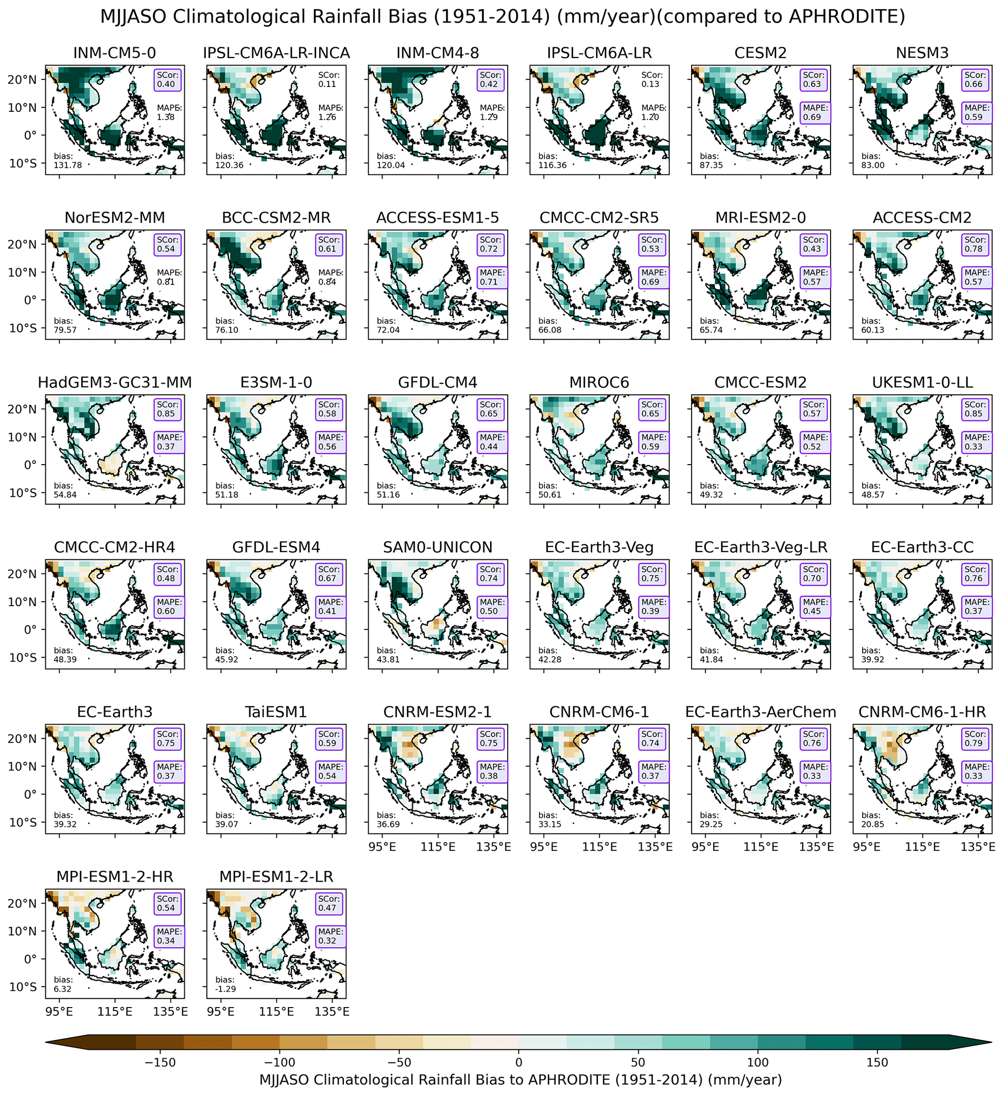
Figure 2 The seasonal climatological (1951–2014) bias (in mm yr⁻¹) for each model against the APHRODITE observational product during the wet season (May–October; MJJASO), ranked from wettest to driest based on regionally averaged bias. The mean absolute percentage errors (MAPEs) and spatial correlations (Scor's) calculated against APHRODITE are shown in the upper-right corner. Values highlighted in purple-coloured boxes indicate values that meet our defined benchmarking thresholds. All analyses are considered at the resolution of the coarsest CMIP6 GCM (i.e. NESM3, ∼ 216 km).

Figure 3 Same as Fig. 2 but for the dry season (November–April; NDJFMA).

3 Results

3.1 Minimum standard metrics (MSMs)

3.1.1 Mean absolute percentage error (MAPE) and spatial correlation (Scor)

We initially assess the performance of CMIP6 GCMs in reproducing the spatial distribution of precipitation using the first two MSMs: MAPE and Scor. Previous studies have emphasised strong seasonal and regional contrasts in rainfall distribution over Southeast Asia (Nguyen et al., 2023). Therefore, we focus on comparing the seasonal climatology (1951–2014) of total rainfall during wet days (e.g. precipitation ≥ 1 mm) between models and APHRODITE for both the wet MJJASO and dry NDJFMA seasons (Figs. 2 and 3, respectively). For MSMs, our strategy is to retain as many models as possible. We establish benchmarking thresholds based on the requirements of downscaling CMIP6 from CORDEX communities and our understanding of reasonable model performance based on current scientific understanding. In particular, GCMs should adequately reproduce the spatial distribution of rainfall without a strong wet or dry bias. In addition, we also identify observational uncertainties through intercomparison of multiple precipitation datasets. Considering variations in model performance across seasons, we also set different thresholds for benchmarking models for different seasons. In particular, due to the better ability of the models to capture spatial variability in precipitation during the dry season compared to the wet season (Desmet and Ngo-Duc, 2022), we adopt a more lenient approach by relaxing our expectation for a spatial distribution metric, setting the Scor threshold ≥ 0.4 for the wet season and ≥ 0.75 for the dry season. However, for the MAPE score, we apply a stricter criterion, as we require models to closely simulate observed rainfall intensity over SEA. For both wet and dry seasons, we set the benchmarking threshold for MAPE at ≤ 0.75. With this threshold, our objective is to identify models capable of capturing the spatial variability in rainfall across at least 40 % (Scor ≥ 0.4) or 75 % (Scor ≥ 0.75) of the domain during wet and dry seasons, respectively, with a wet/dry bias of no more than 75 % compared to observations (MAPE ≤ 0.75) for both seasons.

We first discuss key features of the wet season (MJJASO; Fig. 2). Models are ranked from wettest to driest based on their regionally averaged climatologies (i.e. the average of accumulated precipitation over all land grid points inside the domain). Models that meet our benchmarking thresholds for MAPE and Scor (i.e. calculated against APHRODITE) are highlighted by purple-coloured boxes. In general, CMIP6 GCMs demonstrate a wet bias in terms of regional averages ranging from 6.32 to 131.78 mm yr⁻¹, except for MPI-ESM1-2-LR (−1.29 mm yr⁻¹). However, there is spatial variability in the distribution of wet and dry biases. While most of these models consistently show wet biases over the MC, dry biases are observed in different locations on the mainland across models (e.g. along the west coast in the EC-Earth, IPSL and CMCC families or on the east coast in the CNRM family, as well as in some northern regions such as the MPI family). Among the wettest GCMs, including INM, IPSL, NorESM2-MM and the CESM2 family, the largest biases are predominantly over the MC. Interestingly, most CMIP6 GCMs can capture the spatial variability in rainfall (Scor around or greater than 0.5), except for the IPSL-family simulations (Scor's of 0.11 and 0.13). Using the threshold definitions mentioned above, six models fail to meet these benchmarks, exhibiting obvious grouping by GCM group. For example, IPSL-CM6A-LR and IPSL-CM6A-LR-INCA fail due to their low Scor's (0.13 and 0.11, respectively) and high MAPEs (1.20 and 1.26, respectively). While the INM-CM5-0 and INM-CM4-8 models meet our set expectation in relation to spatial variability, they fail to meet the MAPE threshold due to their overestimation of rainfall across the entire region (e.g. MAPEs ranging from 1.29 to 1.38, respectively). All failed models mentioned exhibit high MAPE values ranging from 0.81 to 1.28.

The corresponding results for the dry season reveal some interesting features (Fig. 3). First, there are substantial similarities in the spatial distribution of climatological rainfall biases across models during this season. CMIP6 GCMs consistently show small biases over Indochina and large wet biases over the MC. A better spatial correlation with observations (i.e. Scor > 0.8) is obtained during the dry season, consistent with previous findings, e.g. CORDEX-CMIP5 RCMs (Nguyen et al., 2022) or CMIP6 GCMs (Desmet and Ngo-Duc, 2022), in highlighting the dependence of model performance on the season. With improved performance in capturing the spatial variation in total precipitation intensity compared to the wet season, all models meet our expected performance in spatial variability. However, INM- and IPSL-family models still fail the MAPE criterion since they exhibit much-higher precipitation intensity than APHRODITE, particularly over the MC. Note that over SEA, APHRODITE is drier than other precipitation products, particularly over the MC (Nguyen et al., 2020).

It is important to note that whether a model passes or fails the benchmarking is strongly dependent on the choice of threshold, as emphasised in Isphording et al. (2024). For instance, more simulations would fail this test if we set a higher threshold for Scor, notably for the MJJASO season case.

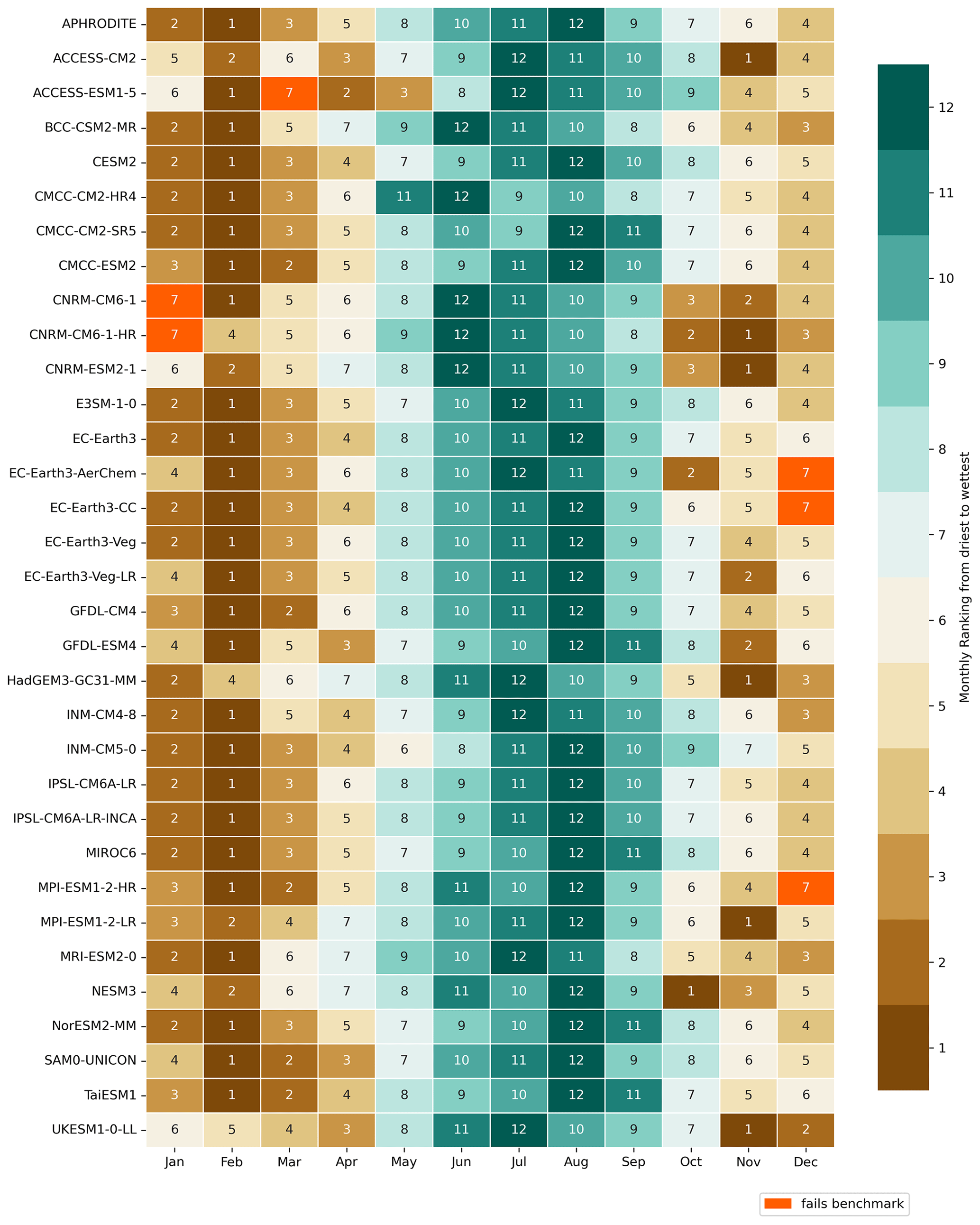
Figure 4 The climatological (1951–2014) average total monthly rainfall over mainland Southeast Asia ranked from driest to wettest for each CMIP6 simulation. Brown shades (1–6) indicate the 6 driest months while teal colours (7–12) indicate the 6 wettest months. The models that failed the benchmarking are highlighted in orange. All analyses are considered at the coarsest CMIP6 GCM resolution (i.e. NESM3, ∼ 216 km).

3.1.2 Seasonal cycle

In this section, we follow the simplified method developed by Isphording et al. (2024) in quantifying the phase and structure of the seasonal cycle. In particular, we rank total monthly precipitation from wettest to driest. We then define the benchmarking threshold such that the 4 wettest and driest observed months must fall within the 6 wettest and driest months simulated by models (Fig. 4).

Overall, most CMIP6 GCMs reproduce the phase well but tend to overestimate precipitation intensity, notably for the observed precipitation peaks during boreal summer (Fig. S3). The INM- and IPSL-family simulations stand out, consistent with the wettest biases observed in spatial patterns (Sect. 3.1.1).

According to the benchmarking threshold definitions, all models meet the benchmark for simulating the 4 wettest observed months. However, six models do not pass the benchmark for simulating the 4 driest observed months, as highlighted in orange in Fig. 4. Specifically, 1 of the 4 driest months according to the APHRODITE dataset (December through March) is ranked as the 6th wettest month (ranked 7th in Fig. 4) by these models.

Figure 5 The observed (top row) and modelled seasonal average total precipitation across Southeast Asia land areas during the wet season (May–October; MJJASO) for the period 1951–2014. The direction of the observed Theil–Sen trend is the benchmark (top row). The Theil–Sen trend line for each of the simulations is plotted in grey if the models fail the benchmark and in purple if they pass. The magnitude of the trend is noted in the top middle, and the results of the Mann–Kendall significance test are noted in the bottom-right corner. Models are sorted based on the magnitude of the spatial average to match the order of Fig. 2. All analyses are considered at the coarsest CMIP6 GCM resolution (i.e. NESM3, ∼ 216 km). All models pass the benchmark.

Figure 6 Same as Fig. 5 but for the boreal dry season (November–April; NDJFMA).

3.1.3 Significant trend

The final MSM aims to explore how rainfall changes over time (Isphording et al., 2024). In this part, we compare the signal of statistically significant simulated and observed trends using the wet (Fig. 5) and dry (Fig. 6) season accumulated precipitation. A Theil–Sen trend is calculated over a 65-year period (1951–2014) and tested at a 5 % significance level using a Mann–Kendall significant test (Kendall, 1975).

There is a significant decreasing trend in observed total precipitation during the wet season (Fig. 5 – top panel), while the dry season has a significant increasing trend (Fig. 6 – top panel). A model fails this benchmark if it exhibits an opposite significant trend to that of the observations. Using this definition, all models pass this benchmark during the wet season, but MRI-ESM2-0 and MPI-ESM1-2-HR fail during the dry season.

Note that the AR6 (Chap. 8, Douville et al., 2021) stated much more confidence in precipitation trends over the MC after 1980. Therefore, we conducted an additional trend calculation (figures not shown) over the 33-year (1982–2014) period for all considered observational products. Although there are differences in the slope of changes among observational products, their direction (not shown) remains the same as the 1951–2014 period.

Table 3 Summary of model performance against the MSMs for precipitation. Models that pass the benchmarks are highlighted in bold.

Table 3 summarises the MSM benchmarking results for the 32 CMIP6 GCMs tested. There are 19 simulations that pass all MSMs and therefore meet the minimum requirements for the purpose of this study.

While the BMF was designed for precipitation, we can also apply the MSMs to other climate variables such as annual mean near-surface temperature (see Figs. S4–S7 and Table S1 in the Supplement). For temperature, we use the APHRODITE daily temperature datasets (version V1204R1 and V1204XR; Yatagai et al., 2012) that span 1961–2015. In general, CMIP6 GCMs show biases in average temperature, with a greater number of GCMs exhibiting cold biases rather than warm biases (Fig. S4). Almost all models succeed in simulating the observed spatial distribution (e.g. Scor's greater than 0.75), phases (e.g. no model fails the benchmarking for the temperature annual cycle; Figs. S5 and S6) and historical trends (e.g. an increasing trend; Fig. S7) in temperature. Overall, models are better at simulating temperature characteristics (e.g. spatial patterns, annual cycles and trends) than precipitation over SEA. Out of the four models that fail the MSMs for near-surface temperature, two INM-family simulations do not meet the expected spatial distribution benchmark (Scor ≥ 0.85), while CNRM-CM6-1-HR and NESM3 show the largest relative errors compared to APHRODITE (MAPE = 0.08). These four models also fail the MSMs for precipitation, as discussed above.

3.2 Versatility metrics – process-oriented metrics

In addition to the MSMs, our aim is to select a subset of GCMs for dynamical downscaling that simulate precipitation mechanisms. Therefore, in the next steps we focus on process-oriented metrics that capture the relationships between precipitation and other variables well.

Figure 7 The spatial distribution of the climatology (1979–2014) of low-level wind circulation during the summer (JJAS; vectors) in ERA5 reanalysis (highlighted by red title) and for individual simulations selected using MSMs. All analyses are considered at the coarsest CMIP6 GCM resolution (i.e. NESM3, ∼ 216 km). Shading indicates the magnitude of the wind (in m s⁻¹). The mean absolute percentage errors (MAPEs) and spatial correlations (Scor's) calculated against ERA5 are plotted in the upper-right corners. The mean of difference in wind direction (MD) referenced to ERA5 is shown in the lower-left corner. Values highlighted in purple-coloured boxes indicate that they meet our defined benchmarking thresholds. Models are ranked from highest to lowest values of MD.

Figure 8 Same as Fig. 7 but for the boreal winter wind (December–February; DJF).

3.2.1 Monsoon wind

We seek to identify models that adequately depict the low-level circulation over SEA during two prominent seasons: boreal summer (June–September; JJAS) and winter (December–February; DJF) by comparing them to ERA5 (Figs. 7 and 8, respectively). To measure the agreement between simulated and observed wind patterns in terms of intensity and direction, we employ three metrics, Scor, MAPE and MD (see Sect. 2.2.2), and we set the benchmarking threshold for each metric in dealing with limited simulations at this versatility stage. In particular, we define the threshold for wind intensity as MAPE ≤ 0.65 to seek models that do not overestimate the amplitude of monsoon wind. In terms of wind structure, we set a stricter benchmarking threshold for Scor of ≥ 0.70, aiming to retain models that adequately represent the distribution of wind intensity across the whole region. Recognising that wind magnitude might be the same at a location but different directions could substantially impact rainfall patterns, we consider a threshold for direction MD of ≤ 20°. This criterion helps to eliminate models where high-speed wind direction deviates significantly from observed patterns.

During summer, ERA5 shows westerly winds flowing from the Bay of Bengal into Indochina, then deviating northward to the northern Philippines (along 10° N). Concurrently, easterly winds from Australia traverse the MC and Papua New Guinea (see Fig. 7). Conversely, in winter, the wind patterns are largely reversed (Fig. 8). The easterly and northeasterly winds from the north pass through the Philippines, reaching the southern coast of Vietnam and the Malaysian peninsula, while westerly winds predominate between the Indonesian islands towards Papua New Guinea.

Overall, the subset of CMIP6 GCMs capture the circulation structure relatively well (Scor's ranging from 0.72 to 0.92 for DJF and from 0.81 to 0.95 for JJAS) but tend to overestimate the wind intensity relative to ERA5, particularly over high-speed wind areas. For example, the westerly component from the Bay of Bengal during JJAS or the easterly component over the MC during DJF is too strong compared to ERA5. These might link with the wet biases discussed in Sect. 3.1. Interestingly, all MSM-selected models for precipitation capture the direction of the main components of JJAS monsoon flow well.

Using the definition of benchmark thresholds mentioned above, all models meet our expectations for wind intensity (MAPE) during the summer season but two fail for the winter season (i.e. MAPEs of 0.79 for CMCC-CM2-HR4 and 0.69 for MIROC6). Interestingly, only one model fails the benchmarking for wind spatial distribution and direction: CNRM-ESM2-1 (MD is 21.67 during DJF; Fig. 8).

3.2.2 Rainfall teleconnections with modes of variability

The rainfall teleconnection for DJF ENSO is examined for two different seasons. We look at the extended summer season of the developing year (MJJASO of year 0) and the boreal spring of the following year (MAM of year +1), while the precipitation–IOD teleconnection is analysed for boreal autumn (SON). To benchmark CMIP6 GCMs, three metrics (HR, MR and FAR; see Sect. 2.2.2) are calculated for each GCM considering the thresholds ≥ 0.5 for HR and ≤ 0.65 for MR and FAR, given the limited number of simulations used at this stage.

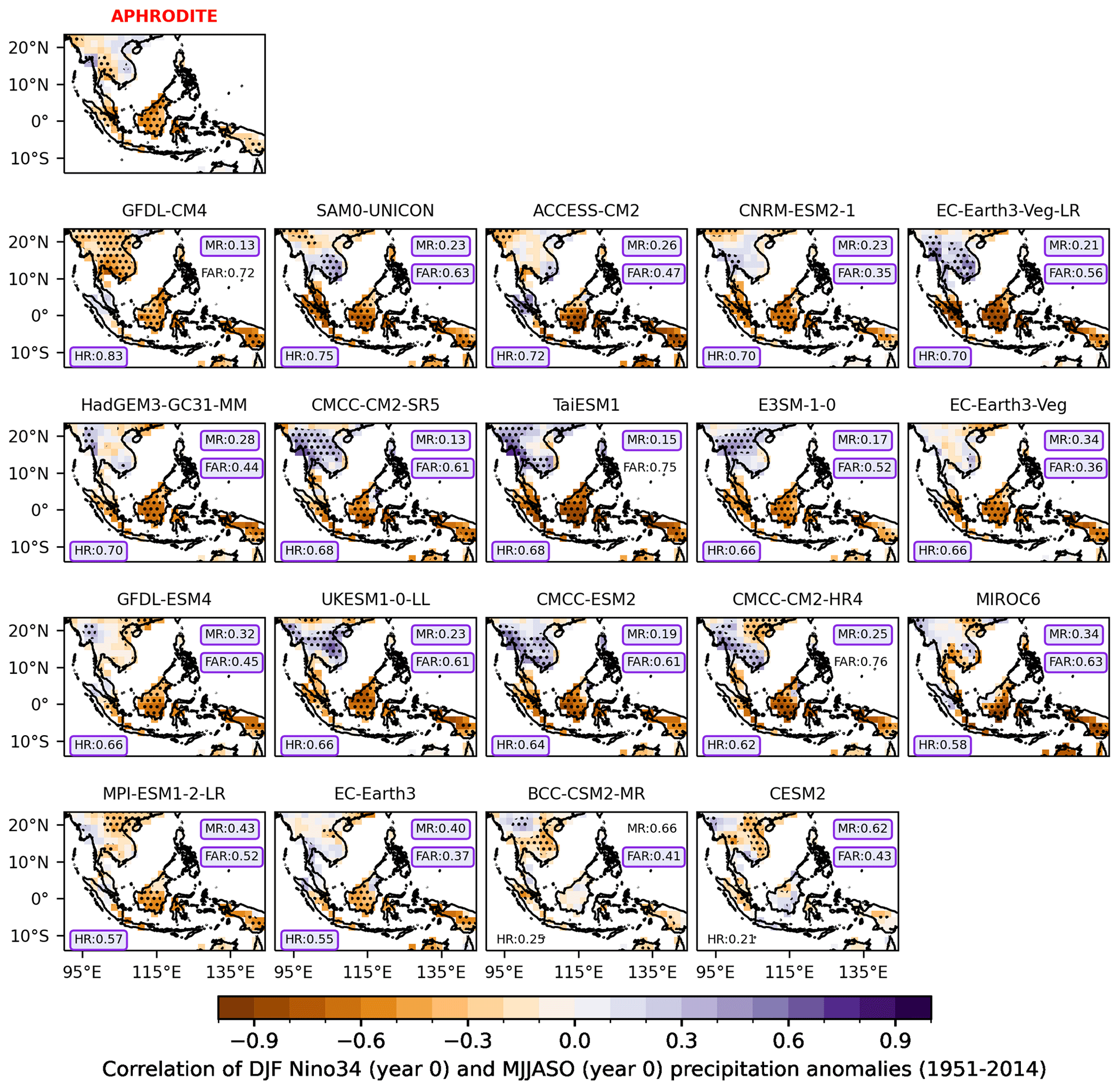
Figure 9 Lead correlation coefficients of the boreal summer (May–October; MJJASO year 0) rainfall with the mature phase of ENSO (December–January–February; DJF year 0 of Niño3.4 indices) for observations from APHRODITE with HadISST: individual CMIP6 GCM models during the period 1951–2014. The stippling indicates the grid points where the correlation coefficient is statistically significant at a 95 % confidence level according to the Student t test. The hit rates (HRs), miss rates (MRs) and false-alarm rates (FARs) calculated against APHRODITE are shown in the bottom-left and upper-right corners. All analyses are considered at the coarsest CMIP6 GCM resolution (i.e. NESM3, ∼ 216 km). Values highlighted in purple-coloured boxes indicate values that meet our defined benchmarking thresholds. Models are ranked from highest to lowest values of HR.

Figure 10 Similar to Fig. 9 but for the lag correlation coefficients of the mature phase of ENSO (December–January–February; DJF year 0 of Niño3.4 indices) with the boreal spring (March–April–May; MAM year +1) rainfall for (top) observations from APHRODITE with HadISST and individual CMIP6 GCM models during the period 1951–2014. Models are ranked from highest to lowest values of HR. All analyses are considered at the coarsest CMIP6 GCM resolution (i.e. NESM3, ∼ 216 km).

Figure 11 Correlation coefficients of the boreal autumn (September–October–November; SON) rainfall with IOD (DMI) for observations from APHRODITE with HadISST and for individual CMIP6 GCMs during the period 1951–2014. The stippling indicates the grid points where the correlation coefficient is statistically significant at a 95 % confidence level according to the Student t test. The hit rates (HRs), miss rates (MRs) and false-alarm rates (FARs) calculated against APHRODITE are plotted in the bottom-left and upper-right corners. Values highlighted in purple-coloured boxes indicate values that meet our defined benchmarking thresholds. Models are ranked from highest to lowest values of HR. All analyses are considered at the coarsest CMIP6 GCM resolution (i.e. NESM3, ∼ 216 km).

The results for observations and CMIP6 GCMs selected from MSMs are shown in Figs. 9–11. The observed teleconnections vary widely by region and season. In general, ENSO-induced summer rainfall variability is dominant over the MC (e.g. Sumatra and Java; Fig. 9), while spring variability is dominant over Indochina, northern Borneo and Philippines (Fig. 10), which agrees with the evolution and seasonal circulation migration mentioned in the previous literature (Juneng and Tangang, 2005; Supari et al., 2018; Wang et al., 2020). On the other hand, IOD-induced rainfall variability is more pronounced during the SON season over the MC (Fig. 11).

CMIP6 GCMs (Fig. 10) demonstrate reasonable accuracy in simulating the spatial distribution of the ENSO teleconnection but tend to overestimate its strength, particularly over regions where observed temporal correlation coefficients are non-significant. During MJJASO of the developing year, most models successfully reproduce significant negative signals over the MC (e.g. high HR values ranging from 0.66 to 0.7 and low MR values less than 0.4). During boreal spring of the following year (MAM of year 1), the ENSO signals in CMIP6 GCMs match the observed pattern better than those during MJJASO of the developing year (Fig. 9), particularly over Indochina. Higher values of HR and lower MRs are found in most CMIP6 GCMs. This is consistent with the previous literature that highlights that GCMs tend to overestimate ENSO variability across much of the equatorial Pacific (McKenna et al., 2020) and produce a poor representation of the ENSO life cycle (Taschetto et al., 2014; McKenna et al., 2020) and interaction between ENSO and IOD (McKenna et al., 2020; Planton et al., 2021). Note that certain models consistently perform well across seasons, such as EC-Earth3-Veg, EC-Earth3-CC, GFDL-ESM4 or HadGEM3-GM31-MM, while others, like BCC-CSM2-MR and CESM2, exhibit less-favourable performance in capturing ENSO teleconnections over the region (Figs. 9 and 10). Eight out of the 19 models, including the EC-Earth3 family, ACCESS-CM2, E3SM1-0, GFDL-ESM4, HadGEM3-GCM31-MM, MPI-ESM1-2-LR, SAM0-UNICON and UK-ESM1-0-LL, meet the ENSO teleconnection benchmark. Among models that did not pass the benchmark, many indicate an overestimation of observed non-significant ENSO signals (FAR) over the mainland during the MJJASO of year 0 (e.g. the FARs of CMCC-CM2-HR, TaiESM1 and GFDL-CM4 are 0.76, 0.75 and 0.72, respectively) or over the MC during MAM of the following year (e.g. the FARs of CMCC-CM2-SR5, EC-Earth3-Veg-LR and CMCC-ESM2 are 0.84, 0.77 and 0.74, respectively).

Interestingly, the precipitation–IOD teleconnection shows some notable similarities among the 18 CMIP6 GCMs considered at the versatility metrics stage (Fig. 11). Most models capture the significant negative correlation over Java and southern Borneo, resulting in high HR values (ranging from 0.58 to 0.75). An exception is CESM2, which produces non-significant signals over the entire region (Fig. 11). Interestingly, models that demonstrate weak performance in simulating ENSO teleconnections (e.g. BCC-CSM2-MR, CESM2 and CMCC-CM2-HR) also struggle to accurately simulate the IOD teleconnection. Using the same threshold definitions as established for assessing the ENSO teleconnection, we identify 14 out of 18 models that pass the benchmarking for IOD teleconnection.

Table 4 Summary model performance against the versatility metrics that focused on precipitation drivers and modes of variability (ENSO and IOD teleconnections). Models that meet or exceed the benchmarks are highlighted in bold. All analyses are considered at the coarsest CMIP6 GCM resolution (i.e. NESM3, ∼ 216 km).

Given the large observational uncertainty, particularly in rainfall estimation over the region (Nguyen et al., 2020, 2022), we apply the BMF using different reference datasets while maintaining a consistent benchmarking threshold definition. This evaluation identifies a similar list of models meeting the minimum standards of performance (Table S1). However, exceptions are noted; for instance, MPI-ESM1-2-LR fails to meet the MSMs when compared with GPCC_FDD_v2018 (short name: GPCC_v2018) but passes with other references. Similarly, NorESM2-MM exhibits varying performance across different observational products. However, even if these two models are included in the subsequent selection steps, they fail to meet one or more versatility metrics. For instance, MPI-ESM1-2-LR fails the IOD–teleconnection benchmark (Fig. 11 and Table 4), while NorESM2-MM fails the ENSO–teleconnection benchmark (Fig. S9).

It is acknowledged that different SST products vary in capturing the teleconnection. Figure S8 indicates the notable similarities among SST products in capturing the response of precipitation with modes of variability over SEA, except for the teleconnection between DJF (year 0) ENSO and MJJASO (year 0) precipitation. However, despite the diversity in SST products, the final selection of models passing the BMF remains the same.

Table 4 summarises the results of benchmarking 19 CMIP6 GCMs selected from the MSM for the versatility metrics. At the point of applying the BMF, we find eight models (ACCESS-CM2, E3SM1-0, EC-Earth3, EC-Earth3-Veg, GFDL-CM4, HadGEM3-GC31-MM, SAM0-UNICON and UKESM1-0-LL) that meet our expectations in simulating precipitation drivers and teleconnections with modes of variability. This could be due to the fact that IOD is an ENSO artefact (Dommenget, 2011).

Figure 12 CMIP6 GCM climate change signal (2070–2099 relative to 1961–1990) over mainland Southeast Asia during (a) the wet season (MJJASO) and (b) the dry season (NDJFMA). The analyses are conducted for the GCMs that simulated at least monthly near-surface air temperature (tas) and precipitation (pr) for the SSP3-7.0 scenario. Note that some models that did not simulate tas or pr for SSP3-7.0 (e.g. E3SM1-0, HadGEM3-GCM31-MM and SAM0-UNICON) are not plotted.

3.3 Future climate change signals and model dependence

In this section, we examine the climate change signals from CMIP6 GCMs that provide at least mean temperature and precipitation data for the Shared Socioeconomic Pathway (SSP3-7.0) scenario across two distinct seasons (see Fig. 12). Note that some models, such as CNRM-CM6-1-HR and EC-Earth3-Veg-LR (listed in Table 1), do not offer the sub-daily data (e.g. atmospheric variables in three dimensions at 6 h intervals) required for dynamical downscaling at the time of writing. Nevertheless, we include these models in our analysis to gain insights into the future climate change responses of CMIP6 GCMs. Interestingly, while temperature projections show general agreement regarding an increasing trend (ranging from 2.1 to 5.1 °C), precipitation projections exhibit large variation in both signal and magnitude (ranging from −4.3 % to 12.9 %). Therefore, we cannot see the linear relationship between the change in regional total precipitation and temperature. Among the eight models that pass our BMF a priori expectations, there are only five models that provide at least data for monthly near-surface temperature (tas) and precipitation (pre), and they are distributed across the wide range of temperature and precipitation signals over SEA. They include the wettest models in both seasons with mid-range projected temperatures, e.g. EC-Earth3 (10 % and 3.6 °C) and EC-Earth3_Veg (8.9 % and 3.4 °C) for the MJJASO season (Fig. 12a), UKESM1-0-LL as the model with the largest increase in temperature (e.g. 5.1 °C during the MJJASO season), GFDL-ESM4 as the model with larger response in precipitation and lower warming (e.g. −11.2 % and 2.5 °C during the MJJASO season), and ACCESS-CM2 as the model with a high-range temperature and mid-range precipitation response (e.g. 4.9 % and 4.2 °C during the MJJASO season).

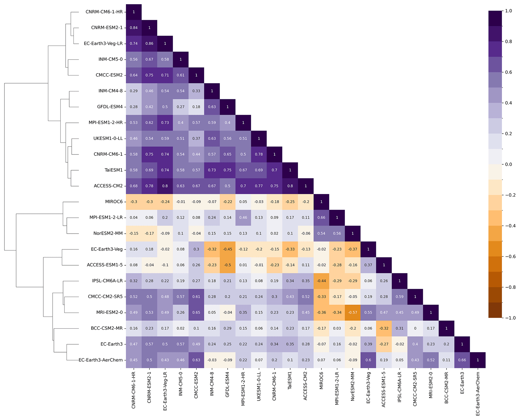
Figure 13 Dendrogram with hierarchical clustering applied to a matrix of spatial correlation coefficients between CMIP6 climate models for the long-term changes (2070–2099 SSP3-7.0 relative to 1961–1990) in total precipitation during the wet season (MJJASO). The matrix is plotted for GCMs that simulated at least monthly near-surface air temperature (tas) and precipitation (pr) for the SSP3-7.0 scenario only. Models are clustered using Ward's linkage criterion.

Figure 14 The same as Fig. 13 but for the dry season (November–April; NDJFMA).

The dendrogram and matrix of spatial correlations between CMIP6 GCMs are shown for Southeast Asia for climatological bias (Figs. S10 and S11) and long-term changes (Figs. 13 and 14) in total precipitation. As before, we focus on the wet (MJJASO) and dry (NDJFMA) seasons. Historical correlations highlight notable similarities between models in historical bias maps (mostly significant and greater than 0.5), except UK-ESM1-0-LL, which shows poorer relationships with other models (e.g. correlation coefficients with other models are less than 0.5; Figs. S10 and S11). However, there is higher independence in projection maps compared with that in historical maps. This interesting feature needs further investigation.

Clustering analysis indicates three main spatial change clusters for the MJJASO season, as shown in the dendrogram (Fig. 13). This indicates similarities in the spatial patterns of the climate change response maps (e.g. correlations greater than 0.5) not only among models from the same families, e.g. among the Met Office GCM-based family (i.e. UKESM1-0-LL, ACCESS's family) and in model families that share the same model components (e.g. the UK-ESM1-0-LL and EC-Earth3 families share the same ocean model, NEMO3.6; Table 1) but also in less obvious families like the CNRM and INM families or the EC-Earth-based and GFDL-based simulations. An exception is EC-Earth-Veg-LR, which appears in different main clusters compared with other EC-Earth-based simulations. As indicated in the MJJASO dendrogram, the BMF-passing models that have data available for dynamical downscaling are in two main clusters, including the EC-Earth3–EC-Earth-Veg–GFDL-ESM4 cluster and the UKESM1-0-LL–ACCESS-CM2 cluster.

Figure 14 indicates two main spatial change clusters in the dry season. Interestingly, some models from the same family (e.g. EC-Earth3 and EC-Earth-Veg) still belong to the same main cluster but span different branches of the dendrogram. This might be related to the different role of internal variability in determining the level of uncertainty for precipitation during different seasons and needs further investigation. Interestingly, among models that pass the BMF, EC-Earth3 and EC-Earth-Veg appear on a main cluster, while UKESM1-0-LL, ACCESS-CM2 and GFDL-ESM4 are in the other main cluster for the NDJFMA dendrogram. This highlights the dependence of the clustering analysis on the season.

We acknowledge that a model's good performance in simulating historical climate conditions does not necessarily guarantee similar accuracy in future climate projections, a well-recognised issue in climate modelling (Herger et al., 2019). However, there are no arguments in the literature suggesting that models with weaker skill in simulating historical climatology perform better in future projections. On the contrary, we believe that models demonstrating good performance in both statistical and process-based metrics are more likely to provide credible future projections, given their proven ability to accurately simulate the physical mechanisms responsible for generating rainfall in the region.

In general, based on our evaluation of model performance, model dependence and future climate change spread, we identify two independent groups of models to use for dynamical downscaling over SEA, that is, EC-Earth3–EC-Earth-Veg and ACCESS-CM2–UKESM1-0-LL. Models from these two groups also offer the atmospheric variables in three dimensions at 6 h intervals required for dynamical downscaling (Table 1). Given the inconsistency of classification of GFDL-ESM4 during different seasons and metrics, we suggest considering GFDL-ESM4 with caution.

4 Discussion

Our results somewhat differ from traditional model evaluation studies like Desmet and Ngo-Duc (2022), which ranks models by evaluation metrics and identifies a list of the best models including EC-Earth3, EC-Earth3-Veg, CNRM-CM6-1-HR, FGOALS-f3-L, HadGEM3-GC31-MM, GISS-E2-1-G, GFDL-ESM4, CIESM-WACCM and FIO-ESM-2-0. First, rather than ranking models, our aim is to retain models that meet our predefined expectations (e.g. benchmarking thresholds). Second, the list of examined models is different since we especially focus on models with a resolution greater than 2° to avoid the impacts of coarser resolutions in GCMs on dynamical downscaling. Furthermore, while Desmet and Ngo-Duc (2022) combine model performance in simulating surface climates (e.g. precipitation and near-surface temperature) and climate processes (e.g. low-level atmospheric circulation), our focus is solely on precipitation, its drivers and teleconnections with modes of variability.

We acknowledge that the list of models passing the BMF might change depending on how the benchmarking thresholds are defined. Isphording et al. (2024) note that the definition of the benchmarking thresholds for the MSMs and versatility metrics can be subjective, and they should be chosen to fit the purpose of the study while incorporating strong scientific reasoning. The strategy employed here involves defining the benchmarking thresholds based on our knowledge of observational uncertainty over the region. In addition, we aim to give each model the benefit of doubt, thus retaining a broad range of plausible future climate change responses. In particular, in the initial step of the BMF framework, we are generous in defining the benchmark threshold for the wet season given the lower model performance compared to the dry season. This approach results in 19 out of 32 models passing the MSMs. Subsequently we employ versatility metrics to cover a more process-based assessment. Given that previous studies have highlighted the overestimation of GCMs in simulating precipitation drivers and their teleconnections and limited possible simulations at this stage, we also set relaxed thresholds for various metrics to maximise the number of models passing the BMF. We feel this is a pragmatic approach to retain a reasonable sample size and explore plausible futures. However, we acknowledge that dynamical downscaling experiments often require significant computing resources and only a small subset of GCMs should be pre-selected. Therefore, we narrow down our selection of 8 GCMs for further assessment using metrics related to model dependency and future climate change spread.

Previous studies suggest the potential impact of smoothing the extreme values when interpolating to coarser resolutions, which might affect the skill score metrics used to measure percentage errors in a simulation relative to a reference (i.e. MAPE). Although we observe a higher number of failed models for the same skill when conducting the BMF at the GCM original resolutions (Table S4), we identify a similar subset of models meeting all minimum performance requirements (Table S4). This suggests that the coarser resolution of ∼ 210 km used for benchmarking is not the main reason behind the results of quantifying model skill used in this study. This is in line with Nguyen et al. (2022), where they demonstrate that model components (e.g. configurations in different schemes) are the main reason behind the model biases rather than model resolution.

The relationship between model structures and model biases is investigated in the model dependency section using cluster analysis. We acknowledge that grouping of models might changes for not only the periods and seasons considered (as discussed in Sect. 3.3) but also the metrics considered. Interestingly, using mean percentage changes as distance measure between models, we identify similar main clusters of EC-Earth3–EC-Earth-Veg and ACCESS-CM2–UKESM1-0-LL among models that passed the BMF (Figs. S12 and S13). This subset of models is suitable for dynamical downscaling over Southeast Asia.

The customised BMF implemented in this study offers a consistent framework for model evaluation across the whole CORDEX-SEA domain. The framework can be further developed and applied extensively to sub-regions of interest, in particular within the upcoming Climatic hazard Assessment to enhance Resilience against climate Extremes for Southeast Asian megacities (CARE for SEA megacities) project of CORDEX-SEA. In this project, each megacity can identify their climate priority and the associated metrics to select a fit-for-purpose subset of models. This framework could also be implemented in impact-related projections over SEA for credible future projections for particular sectors: agriculture, forestry, water, etc.

5 Conclusion

In this paper, we apply the insight gained from the CMIP6 selection process for dynamical downscaling across various CORDEX domains to Southeast Asia by encompassing several critical factors: model performance, model independence, data availability and the spread of future climate change projections.

Rather than exhaustively evaluating all performance aspects of the models in simulating the Southeast Asian climate, our focus is on selecting models that simulate precipitation well, including its drivers and teleconnections, given the high uncertainty in rainfall projections over the region. In addition, we apply a novel standardised benchmarking framework – a new approach to identify a subset of fit-for-purpose models that align with a user's a priori performance expectations. This framework has two stages of assessment: statistical-based metrics and process/regime-based metrics, conducted for both the wet (MJJASO) and dry (NDJFMA) seasons.

From the first step we identify 19 GCMs that meet our minimum criteria for simulating the fundamental characteristics (e.g. bias, spatial distribution, seasonality and trends) of seasonal rainfall. GCMs generally exhibit wet biases, particularly over the complex terrain of the Maritime Continent. These models then undergo a second evaluation, focusing on their ability to simulate climate processes and teleconnections with modes of variability. While these models consistently capture atmospheric circulation and teleconnections with modes of variability over the region, they exhibit a tendency to overestimate their strength. Ultimately, our framework narrows down the selection to eight GCMs that meet our model performance expectations in simulating fundamental characteristics of precipitation, key drivers and teleconnections over Southeast Asia. There are obvious high-performing GCMs from allied modelling groups, highlighting the dependency of the subset of models identified from the framework. Consequently, additional tests on model independence, data availability for SSP3-7.0 and the spread of future climate change are conducted. These tests lead to the identification of two independent groups of models (e.g. EC-Earth3-Veg/EC-Earth3 and ACCESS-CM2/UKESM1-0-LL) that align with our a priori expectations for dynamical downscaling over CORDEX-SEA. It is recommended that only one model from each group be chosen to avoid models that are too closely related.