RASCAL v1.0: an open-source tool for climatological time series reconstruction and extension

The reduction of in situ observations over the last few decades poses a potential risk of losing important information in regions where local effects dominate the climatology. Reanalyses face challenges in representing climatologies with highly localized effects, especially in regions with complex orography. Empirical downscaling methods offer a cost-effective and easier-to-implement alternative to dynamic downscaling methods and can partially overcome the aforementioned limitations of reanalyses by taking into account the local effects through statistical relationships. This article introduces RASCAL (Reconstruction by AnalogS of ClimatologicAL time series), an open-source Python tool designed to extend time series and fill gaps in observational climate data, especially in regions with limited long-term data and significant local effects, such as mountainous areas.

Employing an object-oriented programming style, RASCAL's methodology effectively links large-scale circulation patterns with local atmospheric features using the analog method in combination with principal component analysis (PCA).

The package contains routines for preprocessing observations and reanalysis data, generating reconstructions using various methods, and evaluating the reconstruction's performance in reproducing the time series of observations, statistical properties, and relevant climatic indices. Its high modularity and flexibility allow fast and reproducible downscaling. The evaluations carried out in central Spain, in mountainous and urbanized areas, demonstrate that RASCAL performs better than the ERA20C and ERA20CM reanalysis, as expected, in terms of R², standard deviation, and bias. When analyzing reconstructions against observations, RASCAL generates series with statistical properties, such as seasonality and daily distributions, that closely resemble observations. This confirms the potential of this method for conducting robust climate research. The adaptability of RASCAL to diverse scientific objectives is also highlighted. However, as with any other method based on empirical training, this method requires the availability of sufficiently long-term data series. Furthermore, it is susceptible to disruption caused by changes in land use or urbanization processes that might compromise the homogeneity of the training data. Despite these limitations, RASCAL's positive outcomes offer opportunities for comprehensive climate variability analyses and potential applications in downscaling short-term forecasts, seasonal predictions, and climate change scenarios. The Python code and the Jupyter Notebook for the reconstruction validation are publicly available as an open project.

1 Introduction

The origins of meteorological observation can be traced back to ancient civilizations, where people began to notice patterns in the weather and celestial phenomena. However, it was not until the 17th century that systematic weather observations began in earnest with the development of instruments such as the mercury barometer and the thermometer by scientists Evangelista Torricelli and Daniel Gabriel Fahrenheit (Barry and Chorley, 2009). An early example of this interest in observing the atmosphere using instruments is the Central England Temperature (CET) record (Manley, 1974), which is one of the longest instrumental temperature records in the world, dating back to 1659. It provides a continuous monthly temperature series for the central England region and is often used as a proxy for temperature variations in western Europe. Other examples of early weather monitoring date back to the 18th century, such as the Paris–Montsouris observations in France (Moisselin et al., 2002), the Zentralanstalt für Meteorologie und Geodynamik in Austria (Vienna) (Auer et al., 2007), the Uppsala University observations in Sweden (Bergström and Moberg, 2002), and the earliest observations recorded for the Iberian Peninsula like those starting in Seville (Spain) in 1780 (Domínguez-Castro et al., 2014). Since these first observations began, the number of surface meteorological observatories worldwide has increased significantly, as shown in Fig. 1a.

The critical role played by surface meteorological stations in climate monitoring and research is emphasized by the Intergovernmental Panel on Climate Change (IPCC) in all its assessments and reports (IPCC, 2021). One of the aspects addressed is the need to maintain high-quality and consistent data following high standards of quality assurance and control (Begert et al., 2005). These kind of procedures are essential to ensure that the data collected are homogeneous, accurate, and reliable. Errors or inconsistencies in the data can lead to erroneous climate assessments and predictions (Yang et al., 2005). Another important fact mentioned is the need for a dense network of surface meteorological stations around the globe to provide comprehensive coverage of different regions and climates. Dense monitoring networks are less common in remote or less densely populated regions or where the environmental conditions are too harsh to operate and maintain the instruments (Dinku, 2019; Fan et al., 2020; Schween et al., 2020).

It has been commonly accepted that surface meteorological stations are still the best way to identify long-term trends and variability in climate. They have also proven to be critical for validating and calibrating other atmospheric databases such as those obtained from satellites or remote sensing instruments (Salio et al., 2015; Emery et al., 2001; Huang et al., 2019). They are also a key element for the development and validation of gridded databases obtained by numerical models such as reanalyses (Molina et al., 2021; Bell et al., 2021; Lavers et al., 2022; Bonshoms et al., 2022). More recently, meteorological measurements have become an essential element of machine learning methods applied to atmospheric modeling.

Figure 1 (a) Total number of operative stations from 1850 to 2023. (b) Balance of decommissioned stations in the same period. The negative value means the stations are no longer operative, and the absolute value represents the number of decommissioned stations. (c) Localization of all stations from 1850 to 2023, with operative stations in 2023 marked in blue and decommissioned stations as of 2023 marked in red. Data were obtained from the Global Historical Climatology Network daily (GHCNd, https://www.ncei.noaa.gov/products/land-based-station/global-historical-climatology-network-daily, last access: 15 November 2023).

Due to the important role played by surface observations in climate assessing and weather forecasting, several countries established and expanded their surface meteorological observatories during the 20th century, trying to cover as much territory as possible (Klein Tank et al., 2002), from several thousand surface stations at the end of the 19th century to several tens of thousands at the end of the 20th century (Fig. 1a). However, as mentioned before, the results are very uneven around the world (Fig. 1c), with important areas of the world still under-monitored.

Contrary to what might be expected, the number of surface meteorological stations has not increased in recent decades at a rate that would fill the gaps in the documented under-monitored areas. Rather, the ratio of operational stations has slowed down and decreased since the 1970s (Fig. 1a). As can be seen, the number of decommissioned stations has increased in recent decades in many regions of the globe, disrupting some historical climate time series.

One potential explanation for this decline in the number of surface stations is the advent of satellites as a novel method for observing the weather and climate. Following the launch of the world's first weather satellite, TIROS-1, in 1960, satellite weather observations became prevalent and began to offer a number of advantages over on-site weather observations, as cited in Purdom and Menzel (1996). For instance, they permit global coverage and cost-effectiveness since they do not necessitate an extensive network of ground-based weather stations to cover vast areas. However, satellite weather observations also have limitations. For example, they have difficulties accurately measuring conditions at the Earth's surface, their data availability is highly dependent on cloud cover, they often exhibit long-term instrument drift, and they have calibration issues in remote areas where surface observations are still unavailable.

Another potential factor contributing to this decline is the increasing use of model reanalysis data to conduct climate research (Dee et al., 2014; Hersbach, 2016). Model reanalyses employ a combination of observational data sources, including in situ surface weather observations, satellite data, and others to generate a gridded and consistent dataset of weather and climate information from the past. The resulting datasets are comprehensive, are homogeneous, and have strong climatological consistency. They cover global areas, enabling analysis where in situ data are not accessible. In many cases, reanalyses are used instead of in situ measurements for climate studies. They are certainly useful for studying broad climate patterns and long-term climate trends, and they could theoretically be used to fill gaps or extend the temporal and spatial coverage of observations. However, they suffer significant losses with regards to temporal and spatial resolution, as well as information relating to local phenomena. Global reanalyses have inherent difficulties in providing fine-scale details that are often missed in the physics of the models or are meaningless at the low resolution considered.

Although it may seem that global weather data are fully accessible through the more precise reanalyses available nowadays, there may be a hidden loss of information about local phenomena that only surface weather stations are able to capture. When historical meteorological data are not continued indefinitely or interrupted, many of the resources invested over decades are lost. In addition to these interrupted time series, there are also numerous surface meteorological observation series of good quality around the world as a result of short-term campaigns or very recent initiatives. These time series also provide a wealth of information on local processes, but their short duration is still insufficient for climatological analyses (Durán et al., 2017).

We have global reanalyses that span the entire 20th century and part of the 21st century, with low resolution and limited phenomena. However, these datasets are sufficient to consider the main drivers that force weather and climate at the surface. In contrast, we have sets of interrupted or recent surface measurements that capture local phenomena, but these are too short to conduct climatological analyses. It thus appears feasible to downscale reanalysis data in order to obtain pseudo-observations that can provide the best of both worlds.

Downscaling has been performed since the inception of reanalysis. Two general approaches to downscaling are dynamical downscaling (DD) and empirical statistical downscaling (ESD). ESD relies on observational data to establish empirical relationships between the large-scale fields provided by the reanalysis and the local phenomena seen in the observations (Wilks, 2011; Bürger, 1996; Boé et al., 2006). These are grouped into model output statistics, perfect prognosis, and weather generators (in which analog models are used). On the other hand, DD is achieved by using higher-resolution physical models that account for lower-scale phenomena nested within the reanalysis fields (Lo et al., 2008; Durán and Barstad, 2018; Wang et al., 2021).

Numerous papers scrutinize the advantages and disadvantages of the various methods (Hewitson and Crane, 1996; Hanssen-Bauer et al., 2003; De Rooy and Kok, 2004). As a rule of thumb, empirical techniques are generally less computationally intensive than physical downscaling and may yield better results at a lower cost. However, empirical downscaling is only feasible when a sufficiently long and uniformly collected dataset of observations is available. Assuming the hypothesis that there is a connection between the large-scale phenomena shown by the reanalysis and the local phenomena captured by the observations is also essential.

Regardless of the chosen downscaling method, combining reanalysis and surface observations to create long and homogeneous time series requires a significant amount of effort. Setting up a dynamic regionalization system can be expensive in terms of both computation and human resources, but even a relatively simple statistically based regionalization method entails a learning curve that may discourage or slow down certain climate studies.

This work introduces and explains RASCAL v1.0 (Reconstruction by AnalogS of ClimatologicAL time series), an open-source tool for climatological time series reconstruction and extension using ESD. The primary goal of RASCAL is to promote and accelerate rigorous climate research in regions where surface meteorological observations are insufficient for climate analysis and where relevant regional and local meteorological processes can only be captured through in situ observations. RASCAL could prove highly beneficial for mountain climate research and other areas with unique microclimates, such as river valleys, forests, caves, or canyons.

This study is organized as follows: Sect. 2 provides a detailed description of the implemented method, while Sect. 3 describes the model structure and implementation. In Sect. 4, we evaluate the performance of the package by downscaling the daily maximum and minimum temperatures and precipitation of four stations near a mountainous region in central Spain. We draw final conclusions and important remarks in Sect. 5.

2 Methods

RASCAL is based on an ESD type known as an analog model or weather generator. This is a widely used technique in climate research (Zorita and Von Storch, 1999). It is based on the premise that large-scale atmospheric conditions tend to produce comparable local weather patterns, allowing the prediction of local conditions for a day without real-time observations. This is done by identifying an analog day from general circulation models (GCMs), such as reanalyses, and assigning its local conditions. This approach allows the study of climate variability over an extended time frame, providing valuable perspectives on long-term patterns and connections between different geographic locations, while also incorporating important local factors in the analysis (Hidalgo et al., 2008; Benestad, 2010; Abatzoglou and Brown, 2012; Saavedra-Moreno et al., 2015; Shulgina et al., 2023).

The analog method is a nonlinear technique that relies on the identification of strong statistical relationships between two fields: the predictor variable extracted from GCM products and the predictand variable obtained from local historical observations. To predict an atmospheric feature (the predictand) for a given day, this method searches for the day with the most similar predictor field in the historical record and uses its atmospheric features to make a prediction, allowing the reconstruction of missing data points (Lorenz, 1969; Horton et al., 2017).

To incorporate the relationship between large-scale meteorological patterns and local weather, the analog method is often combined with principal component analysis (PCA). PCA reduces the high dimensionality of the atmospheric phase space by generating an orthogonal basis of vectors that represent the main directions of variability. As a result, only a limited set of m coefficients, called principal components (PCs), are required to represent the atmospheric state (Wilks, 2011). The resulting set of m coefficients of the PCs at time t are considered the predictor $\mathbf{X}\left(t\right)=\left(X_{\mathrm{1}}\right(t),X_{\mathrm{2}}(t),\mathrm{\dots },X_m(t\left)\right)$ for the local predictand Y(t). For a given day t, the objective is to identify N historical days $t_{\mathrm{1}},t_{\mathrm{2}},t_{\mathrm{3}},\mathrm{\dots },t_N$ such that the predictor X(t) is similar to the predictors X(t_i). The similarity between the predictors in the historical record X(t_i) and the predictor of the day to reconstruct X(t) is measured with the Euclidean distance.

$$\begin{array}{}\text{(1)}& d_X(t,t_i)=\Vert \mathbf{X}\left(t\right)-\mathbf{X}\left(t_i\right)\Vert \end{array}$$

The N days with the smallest distance d_X(t,t_i) constitute an analog pool. Various similarity methods can be used to select the best analog $\widehat{Y}\left(t\right)$ or group of analogs from the pool. The most straightforward method is to choose the day t_i that has the smallest distance d_X(t,t_i) and that is the closest day in the PC space. However, similar synoptic patterns can sometimes produce different local weather if the role of other variables or more complex phenomena is not taken into account. Therefore, assigning the day with the most similar predictor field pattern as the analog day may not always be accurate. To avoid making the reconstruction method too complex, one solution is to select the N closest days from the pool of analogs instead of just one. Then, perform a weighted average of the predictand Y(t_i) by the square of the distance in space of the PCs of those days:

$$\begin{array}{}\text{(2)}& \widehat{Y}\left(t\right)={\displaystyle \frac{\mathrm{1}}{N}}\sum _{i=\mathrm{1}}^N{w}_{i}Y\left(t_i\right),\end{array}$$

where the weight w_i is

$$\begin{array}{}\text{(3)}& w_i={\displaystyle \frac{\frac{\mathrm{1}}{d_X(t,t_i{)}^{\mathrm{2}}}}{{\sum }_{j=\mathrm{1}}^N\frac{\mathrm{1}}{d_X(t,t_j{)}^{\mathrm{2}}}}}.\end{array}$$

This way, the days with a more similar synoptic pattern have more presence in the average, while also considering possible phenomena that have not occurred on the closest day but on the other similar days.

Averaging can impact the distribution of the variable by smoothing the data and removing extreme values. To preserve extremes while still accounting for possible phenomena beyond the similarity of synoptic patterns, bias reduction methods such as quantile mapping can be used. This technique employs a “mapping variable” Z(t) and examines the quantile of the day to reconstruct Q(Z(t)) in the distribution of this variable in the analog pool $\left(Z\right(t_{\mathrm{1}}),Z(t_{\mathrm{2}}),\mathrm{\dots },Z(t_N\left)\right))$. The method first examines the distribution of the predictand variable in the analog pool $\left(Y\right(t_{\mathrm{1}}),Y(t_{\mathrm{2}}),\mathrm{\dots },Y(t_N\left)\right))$ and selects the day t_i that occupies the same quantile as the best analog.

$$\begin{array}{}\text{(4)}& \widehat{Y}\left(t\right)=Y\left(t_i\right),\text{when}Q\left(Y\right(t_i\left)\right)=Q\left(Z\right(t\left)\right)\end{array}$$

This approach improves the representation of extreme events. However, it is crucial to note that the mapping variable must have a strong correlation with the predictand variable. One possible solution is to use the reanalysis predictand variable as the mapping variable.

The analog method fundamentally involves the reorganization of observed time series data, aiming to maintain the statistical characteristics of the original dataset. The efficacy of this method relies on ensuring that the downscaling and training periods exhibit a comparable climatic context (Zorita et al., 1995). The reconstruction capability of the analog method is constrained by the temporal extent and accuracy of historical observations. This means that it cannot replicate unobserved events and, therefore, cannot reproduce new record values in the context of climate change. However, its utility becomes pronounced in scenarios where external climate forcing induces shifts in the frequency of observed phenomena. In essence, it serves as a valuable tool for discerning alterations in the occurrence patterns of documented events.

3 Model structure

Empirical downscaling techniques involve laborious steps that must be carefully addressed to ensure the quality of the local climate series reconstructions, as pointed out in Boateng and Mutz (2023). RASCAL is a Python library that implements the analog method in a clear and simple way. It is an object-oriented library with four main blocks or classes: Station, Predictor, Analogs, and RSkill. This library is a valuable complement to other empirical downscaling libraries, such as pyESD from Boateng and Mutz (2023), which is based on machine learning downscaling methods that focus on generating monthly time series. RASCAL is based on classical statistical methods, which produce results that are easier to interpret physically, and additionally, it is more focused on daily-resolution reconstructions rather than monthly, which allows for the calculation of relevant daily climate indices. This section describes these components and their implementation workflow, as illustrated in Fig. 2.

3.1 Station class

The analog method requires (1) homogeneous time series of observational data and (2) a reanalysis dataset or GCM product that covers both the period to be reconstructed and the period of historical observations. The Station class retains the information about the historical record, including metadata about the observation point such as its name, elevation, latitude, and longitude, as well as the observational data of the variable to be predicted. The historical record must have a daily to sub-daily resolution, and it is assumed to be homogeneous. The data are preprocessed to extract the desired meteorological variable, such as maximum, minimum, mean, or total accumulated, in the form of selected daily quantities.

3.2 Predictor class

The analog method has the benefit of low subjectivity due to its limited parameters for adjustment (Wetterhall et al., 2005). However, selecting and processing the predictor correctly constitute a crucial step for achieving accurate local weather reproduction. The selection should be based on our knowledge of atmospheric dynamics and the local climate of the study area, as pointed out by other authors (Boateng and Mutz, 2023). After selecting a predictor variable that is expected to have a strong relationship to the predictand variable, for instance its main large-scale forcing field, and that is relevant to the proposed scientific question, it is necessary to choose a predictor field domain that can identify relevant synoptic patterns for the study area. These fields should be carefully grouped for each day. Although the analog method is based on recognizing patterns in a single predictor field, it is possible to use multiple variables within the same field. To use vector fields with multiple components or to include different variables, it is necessary to construct a composite field by concatenating each variable on the longitude axis. This results in a single field with dimensions of time, latitude, and number of components × longitude.

These steps are implemented in the class Predictor. It takes as input the paths to the files of the chosen predictor and allows selecting the limits of the field domain and grouping them for each day, taking only 1 h, or computing the sum or the average of all the available hours. The composite field is obtained when the mosaic option is set to True and more than one different variable is detected within the files of the input paths.

Once the predictor field is chosen, the PCA is performed. The PCA is implemented as the method Predictor.pcs(). To perform the PCA it is necessary to calculate the anomalies of the predictor field. In this method it is possible to choose the months of each season and the number of seasons, the number of principal components to be used, and the scaling of the PCs. This scaling will subsequently influence the selection of a pool of the N closest days. This method wraps the Python library EOFs (Dawson, 2016) using xarray (Hoyer et al., 2020), so it has its scaling options, which are (0) un-scaled principal components, (1) principal components scaled to unit variance (divided by the square root of their eigenvalue), and (2) principal components multiplied by the square root of their eigenvalue.

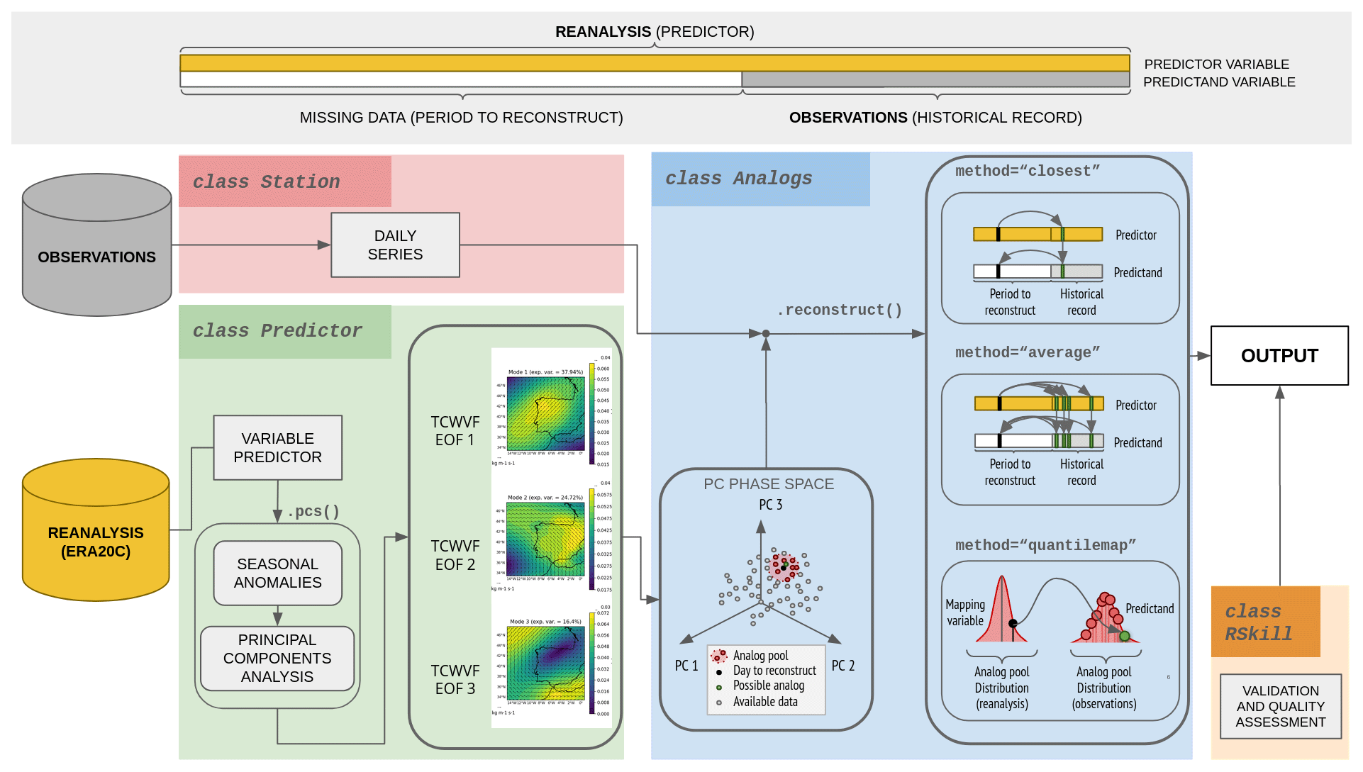
Figure 2 RASCAL main features and workflow. The colored boxes highlight the principal classes, and within them, the featured methods and objects are shown. An example of the EOFs obtained for the total column water vapor flux (TCWVF), used as a precipitation predictor, is included in the Predictor class box.

3.3 Analogs class

After establishing the predictor and determining its synoptic patterns via PCA, the next step is to search for a set of days with similar synoptic patterns for each day, known as the analog pool. After determining the analog pool, the days without observations are reconstructed using one of the following similarity methods: (1) the “closest” method, which selects the closest day in the space of the PCs; (2) the “average” method, which calculates the weighted average of the N closest days; or (3) the “quantile map” method, which chooses the day that corresponds to the same quantile as the day to be reconstructed in another variable called the mapping variable. These steps are implemented in the Analogs class. This object is fed by the historical observations from the Station object and the PC time series of the Predictor object. This object allows the user to select the number of analog days in the pool as pool_size; the number of days to exclude from the pool when testing the reconstruction performance; and whether to exclude the previous, posterior, or both days as vw_size and vw_type arguments. Additionally, it allows the selection of the similarity method. To use the quantile mapping method a mapping variable is required. This variable must be a time series from the reanalysis dataset in the grid point of the station. The Predictor class can be used to obtain this information by setting the domain limits to the station's localization, which is saved in the Station object.

3.4 RSkill class

To assess the quality of a reconstructed time series, it is necessary to clearly state its goal beforehand. RASCAL is designed to produce daily reconstructions to calculate relevant indices, such as days above the 0 °C isotherm or the length of dry spells. However, it is not necessary for the daily reconstructions to be completely in phase with the daily observations when the objective is to evaluate these quantities at coarser temporal resolutions, such as monthly, seasonal, or annual. It is sufficient that their behavior and statistical properties are well-reproduced at these coarser temporal resolutions. To evaluate the skill of the reconstructions, RASCAL is equipped with a skill evaluation class called RSkill. This class contains functions to evaluate the behavior of the reconstructions and assess their added value compared to using the reanalysis data alone. The skill metrics and diagrams included are the following: Taylor diagrams, quantile–quantile diagrams, time series and annual cycle plots, root mean squared error (RMSE), correlation coefficient (R²), mean bias error (MBE), MSE-based skill score (where MSE is the mean squared error), Heidke skill score (HSS), and Brier score (BS).

The MSE-based skill score (Wilks, 2011) is given by

$$\begin{array}{}\text{(5)}& {\mathrm{SS}}_{\mathrm{MSE}}=\mathrm{1}-{\displaystyle \frac{\mathrm{MSE}}{{\mathrm{MSE}}_{\mathrm{r}}}},\end{array}$$

where MSE is the MSE of the reconstruction and MSE_r the MSE of the reference model, in this case the reanalysis. Therefore, the SS_MSE can be interpreted as the relative error reduction of the reconstruction compared to the reanalysis series.

The Heidke skill score (HSS) is implemented in order to assess the performance of the analog method in predicting days where the predictand is above or below a certain threshold compared to the reanalysis, based on a contingency table analysis. The HSS scores events based on their occurrence or absence and determines whether the performance of the tested model is superior to that of the reference model. The HSS is defined as

$$\begin{array}{}\text{(6)}& \mathrm{HSS}\left(r\right)={\displaystyle \frac{r-r_{\mathrm{r}}}{\mathrm{1}-r_{\mathrm{r}}}},\end{array}$$

where r is the proportion of correct forecast (true positive and true negative) of the reconstructed series and r_r the proportion of correct forecast of the reanalysis. The proportion of correct forecast is expressed as

$$\begin{array}{}\text{(7)}& r={\displaystyle \frac{a+d}{a+b+c+d}},\end{array}$$

where a is the number of times that an event is forecasted and observed (true positive), b the number of times that is forecasted but not observed (false positive), c the number of times that is observed but not forecasted (false negative), and d the number of times that is neither forecasted nor observed (true negative).

This score condenses the information on whether the tested model performs better that the reference model with a number in the interval $(-\mathrm{\infty },\mathrm{1}]$. A model that perfectly reproduces the observations gets a score of 1; if it performs as well as the reference model it gets a score of zero, and if the model performs worse than the reference model it gets negative scores.

3.5 RASCAL implementation

Although RASCAL is designed as a Python library, the GitHub repository contains scripts that allow performing reconstructions and skill evaluations without the need to write a script. The multiple_runs_example.py script demonstrates a workflow that reconstructs several stations and variables using different values for the parameters including analog pool size, number of days in the weighted average, and similarity method. There is also a Jupyter Notebook available, named RASCAL_evaluation.ipynb, which evaluates the skill of the reconstructions for daily, monthly, and annual series.

4 Application examples

To test RASCAL performance, we tested the skill of the reconstructions of maximum and minimum temperature and daily precipitation at four different surface stations in the vicinity of the Central System of the Iberian Peninsula (Spain), as shown in Fig. 3. This mountain range is of vital importance as it is the main contributor to the hydrological resources of central Spain due to the high levels of rainfall and snow runoff in spring. This area has been the subject of several studies by authors in recent years (Durán et al., 2013, 2015; Durán and Barstad, 2018; González-Flórez et al., 2022). The reader can refer to these previous works in order to understand the importance of having long time series in this area.

4.1 Observational data

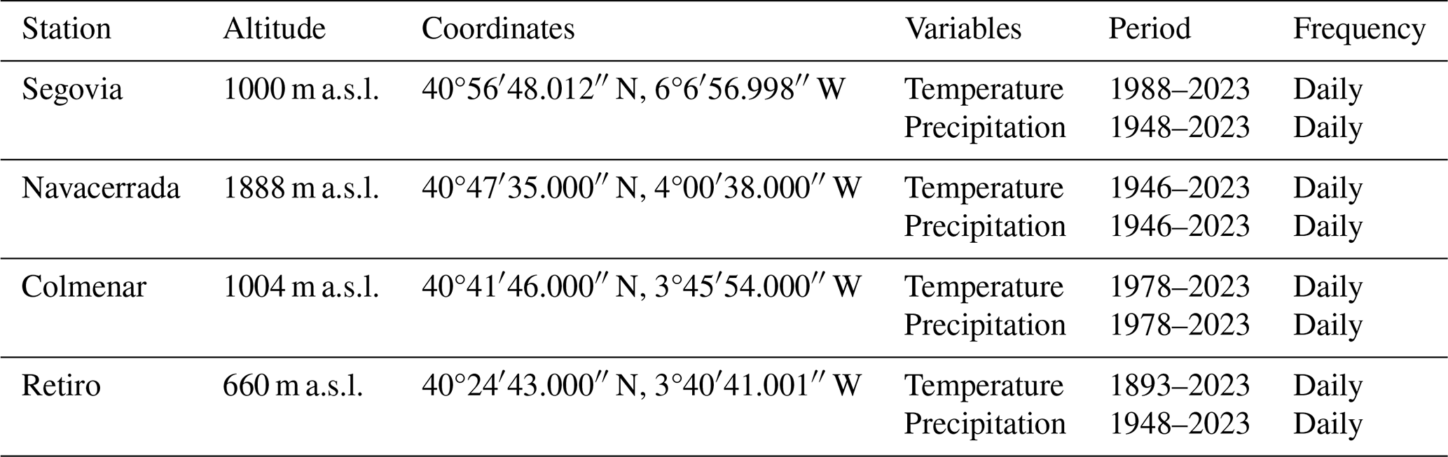
The surface stations used are summarized in Table 1. All of the stations belong to the Spanish Meteorological Agency (AEMET; http://www.aemet.es, last access: 13 September 2023), which has conducted high-quality observations of temperature and precipitation since 1893 and 1948, respectively, for the case of Retiro station located in Madrid. The Navacerrada station is the highest one, situated at 1888 m a.s.l. in the core of Sierra de Guadarrama, an area that has been kept almost unaltered since its installation in 1946. Stations Segovia and Colmenar are located on the northern and southern slopes, respectively, of this mountain massif (Fig. 3). This set of surface meteorological stations was selected based on their long historical records, on the variety of their orography and environments, and on the deep knowledge of this area due to previous research carried out by the authors of this work. Furthermore, they spread across a wide range of altitudes. Of the four datasets, two are particularly long: Retiro and Navacerrada.

Observations have been available at Navacerrada station since 1946. The whole region has remained practically unchanged since then, making it a valuable resource. In contrast, the Retiro station is located in the heart of the city of Madrid, which has undergone significant growth, particularly since the 1960s.

This set of observations can serve as a suitable test bed for evaluating the strengths and weaknesses of RASCAL and its working hypotheses.

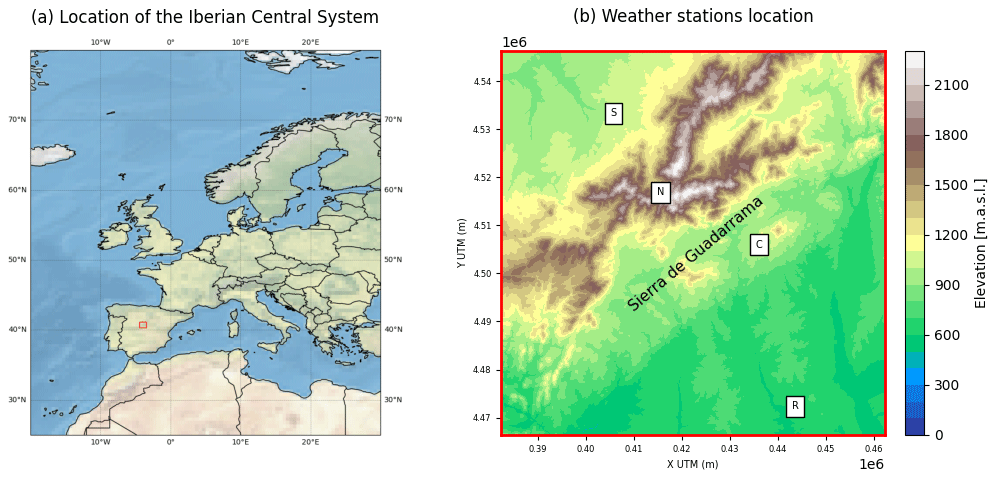
Figure 3 (a) Location of the Iberian Central System. (b) Locations of sites used in this example of application, these being S (Segovia), N (Navacerrada), C (Colmenar), and R (Retiro).

Table 1 Observational data used.

4.2 Reanalysis data

The reconstruction of the time series was performed using ECMWF reanalysis data. Specifically, ERA20C data for the temperature and ERA20CM ensemble data for the precipitation (Poli et al., 2016) were used for the period from 1900 to 2010, with a spatial resolution of 0.75° × 0.75° and a temporal resolution of 3 h.

Principal component analysis was conducted for each season (DJF, MAM, JJA, and SON) individually using geopotential height (GpH) data at 925 hPa as a temperature predictor and TCWVF as the precipitation predictor. The quantile map method used the 2 m temperature and TCWVF to search for analogs in the dataset as the mapping variables. The selection of these predictors was based on their previous use in identifying circulation weather types for precipitation and extreme snow events in the study region, as reported by Durán et al. (2015) and González-Flórez et al. (2022).

4.3 Model evaluation

The reconstructions were performed for all stations using all three similarity methods and varying values of pool size and number of days to average in the average method to account for the possible sensitivity of the results to these parameters. To evaluate the quality of a reconstruction, it is necessary to determine the similarity of the time series to the observations. However, in climate studies it may be more relevant to consider the statistical characteristics of the series. Therefore, it may be more effective to evaluate the ability to reproduce daily distributions, seasonality, seasonal and interannual variability, and relevant indices, such as the number of days below 0 °C or days of precipitation above a certain threshold. RASCAL evaluates the effectiveness of reconstructions for use in climate studies. It assesses the behavior of time series for maximum and minimum temperature, as well as precipitation, and their statistical properties. Additionally, it compares the performance of using the analog method versus using reanalysis data to reproduce observations. To compare its performance against the reanalysis, the temperature data from the reanalysis were corrected with the elevation using the environmental lapse rate (−6.5 °C km⁻¹).

RASCAL includes options to cross-validate when generating the reconstructions. To test the performance of the model in reconstructing gaps in the series and extending to periods distant from the observation period, validation windows are created. These moving windows of N days are taken around each day to be reconstructed, as these are the days that are likely to have the most similar large-scale pattern to the target day and therefore contain the most possible analogs. Excluding these days removes both the large-scale patterns and their associated local meteorological times from the pool of analogs, allowing a better evaluation of the performance of the model and each reconstruction method. For this application case, we excluded 60 d, the 30 d before and after each target day.

4.3.1 Time series skill

Taylor diagrams were implemented in RASCAL to assess the agreement between the reconstructed time series and the observed data. As illustrated in Figs. 4, 5, and 6, these diagrams provide a visual representation of the analysis, displaying the standard deviation and correlation of each time series in comparison to the reference observations.

As depicted in Fig. 4 the precipitation reconstructions outperform the reanalysis precipitation in all the cases for both total monthly and total yearly precipitation. Monthly reconstructions yield better results than the yearly series, with correlation coefficients ranging from 0.4 to 0.8, whereas the yearly series ranges from 0.2 to 0.7. However, for both cases, the reanalysis only shows correlations of 0.4 at best and negative correlations at worst (not visible in the diagram). Panels (c), (f), (i), and (l) display the yearly time series in water years (from October to September), comparing the observations with the reanalysis ensemble and the best reconstruction. The chosen reconstruction has a good correlation coefficient and a standard deviation close to the observations. These panels demonstrate that the correlation and standard deviation are better than the reanalysis and that biases are corrected. An example that illustrates this point is Navacerrada (Fig. 4i), where the reanalysis dry bias may be attributable to a smoothed reanalysis orography that hampers orographic precipitation, an important contributor to total precipitation in this region (Durán et al., 2017).

As evidenced in the difference in the location of points of the same color in the Taylor diagrams, the reconstructions are somewhat sensitive to the pool size selection, as one method with different pool sizes can produce series with different correlations than the observations and standard deviations. However, this sensitivity is not significant enough to be considered a critical determinant in the simulations. Therefore, adjusting this parameter can be useful for subtle modifications.

Additionally, the Taylor diagrams demonstrate how different scientific questions may require different similarity methods. While “average10” shows the strongest correlations, “quantilemap100” exhibits standard deviations closest to the original series, resulting in more similar distributions. Therefore, the choice of reconstruction methods may depend on the specific goals that led to the reconstruction process.

Figure 4 Precipitation time series reconstruction skill for all the stations. The left panels (a, d, g, j) show the Taylor diagrams of the monthly total precipitation series. The central panels (b, e, h, k) show the Taylor diagrams of yearly total precipitation series. The right panels (c, f, i, l) show the time series of observations, reanalysis, and the selected best-performing reconstruction. In the precipitation case the yearly series are based on water years beginning in October and ending in September.

Figure 5 illustrates that the reconstructions of maximum temperatures yield better results than those of precipitation, with correlation coefficients above 0.93 for the monthly mean maximum temperature series and between 0.3 and 0.9 for the yearly mean maximum temperature series. The reanalysis exhibits a very similar behavior to the quantile map reconstructions for this variable, but the latter consistently shows a slight improvement in correlation or standard deviation. The time series in Fig. 5c, f, i, and l show that although the behavior of the reanalysis is very close to the observations, the reconstructions correct the bias for all the stations, even when the reanalysis was corrected with the elevation.

Maximum temperature reconstructions exhibit less agreement between different similarity methods but demonstrate more consistent outcomes for different pool sizes when compared to the precipitation reconstructions. In this case, the quantile map method is recommended for reconstruction over the closest and average methods.

Figure 5 Maximum temperature time series reconstruction skill for all the stations. The left panels (a, d, g, j) show the Taylor diagrams of the maximum temperature monthly mean series. The central panels (b, e, h, k) show the Taylor diagrams of yearly mean series. The right panels (c, f, i, l) show the time series of observations, reanalysis, and the selected best-performing reconstruction.

In Fig. 6a, d, g, and j, the monthly mean minimum temperatures exhibit a similar behavior to the maximum mean temperatures in Fig. 5a, d, g, and j, with correlation coefficients above 0.9 and a slight improvement in the correlation and standard deviation compared to the reanalysis. The yearly mean series (Fig. 5b, e, h, k) also show moderate improvements compared to the reanalysis, with correlations ranging from 0.3 to 0.9. The quantile map method was found to be the most effective for reconstruction. The bias corrections are apparent in Fig. 6c, f, i, and l.

It should be noted that the reconstruction of Retiro in Fig. 6l shows a peculiar behavior, overestimating the mean minimum temperatures before 1945, followed by an underestimation of the temperatures thereafter. This effect does not appear in the maximum temperature reconstructions in Fig. 5l; a possible hypothesis is that this is due to the progressive urbanization of Madrid, where Retiro is located in the city core. This urbanization leads to a change in the land use and to an increase in the heat island effect, which mainly affects the increase in minimum temperatures (Yagüe et al., 1991). This induces a change in the relationship between the local scale and the synoptic scale and therefore in the relationship between the predictor and the predictand, ultimately affecting the temperature trends.

Figure 6 Minimum temperature time series reconstruction skill for all the stations. The left panels (a, d, g, j) show the Taylor diagrams of the maximum temperature monthly series. The central panels (b, e, h, k) show the Taylor diagrams of yearly series. The right panels (c, f, i, l) show the time series of observations, reanalysis, and the selected best-performing reconstruction.

4.3.2 Distributions

To evaluate the statistical properties of a reconstruction, we first examined the distributions of the daily time series in comparison to the observations. Figure 7 displays the quantile–quantile plots of the daily time series for maximum and minimum temperature, as well as precipitation. These plots illustrate the values assigned to the same percentiles for the distributions of the reconstructed and observed time series. When the distributions are identical, the points align along a 45° line. The distribution of the observations is well-represented by the closest and quantile map methods, as shown in the first row of Fig. 7. However, the average method affects the extreme values as expected, narrowing the distribution further as the pool size increases. The poor performance of the reanalysis in representing precipitation distributions is also evident, as it exhibits a skew towards lower values. All methods show a high alignment with the observed data regarding maximum and minimum temperatures, with a slight narrowing in the distribution for the average methods. The impact of bias correction compared to the reanalysis is prominently noticeable in these variables as well.

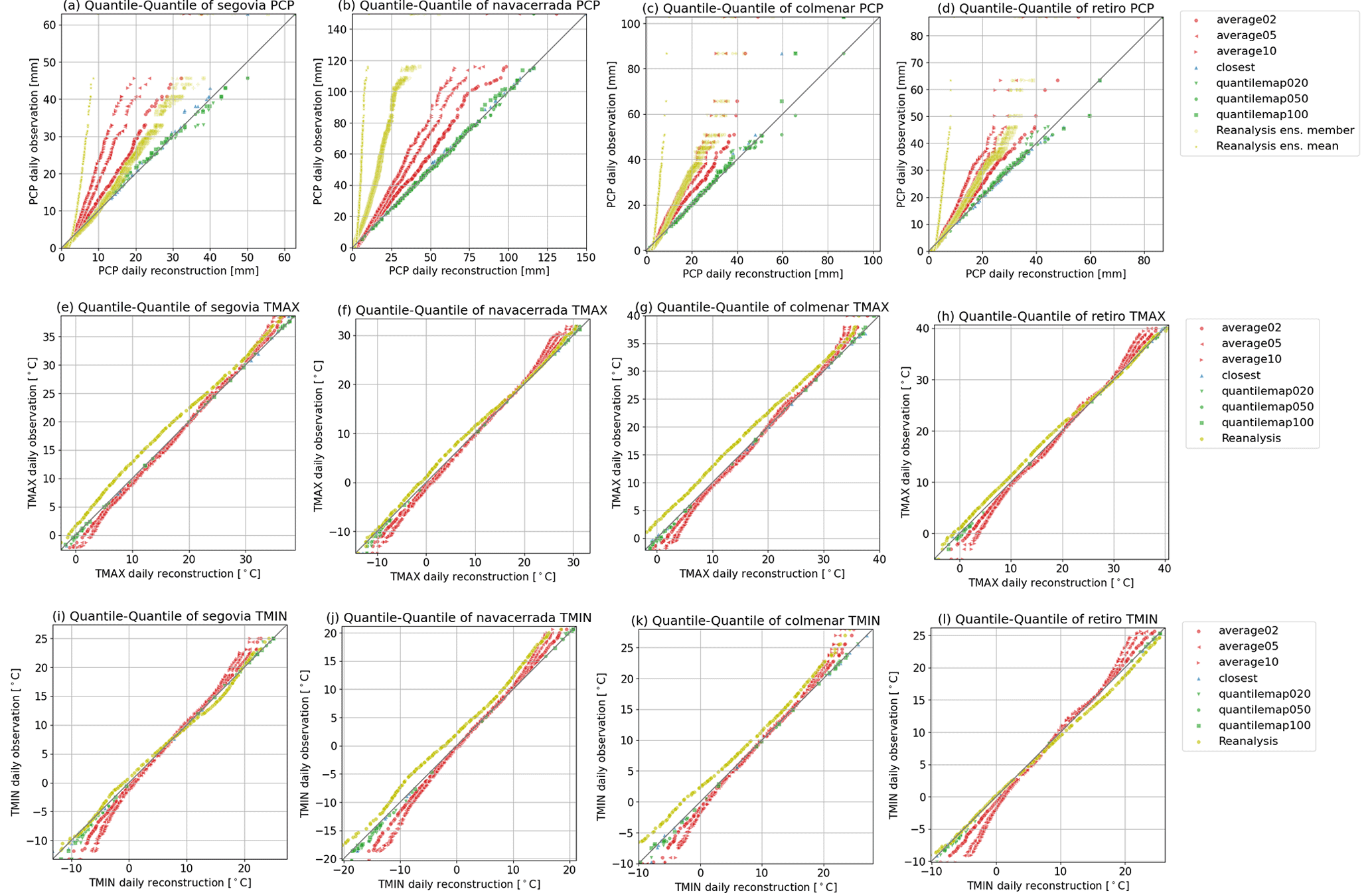
Figure 7 Quantile–quantile plot of the daily time series for all the stations (from left to right) including all the reconstructions and the reanalysis. The first-row panels (a, b, c, d) are for the precipitation, the second row (e, f, g, h) for the maximum temperature, and the third row (i, j, k, l) for the minimum temperature.

4.3.3 Seasonality

Understanding the seasonality of meteorological variables is crucial for climate studies as it enables the identification of recurring patterns and trends throughout the year. As shown in Fig. 8, the seasonal cycles of total monthly precipitation and monthly standard deviation reveal that the reconstructions generally reflect the observations more accurately than the reanalysis. Notably, the quantile map method shows better performance from January to June, while the closest and average methods work better from July to December. These differences between methods are more pronounced in MAM and SON, which are the months of highest variability (Fig. 8e, f, g, h). The standard deviation is well-captured by the quantile map method, with exceptions noted in February and November. Navacerrada once again emerges as the station that benefited the most from the reconstructions. It exhibits the most similar precipitation cycles and standard deviation, outperforming the reanalysis.

Figures 9 and 10 illustrate the annual cycles for maximum and minimum temperatures, respectively. The quantile map method outperforms the closest and average methods, as evidenced by the standard deviation, and is therefore recommended. These results demonstrate that RASCAL is more effective than the reference reanalysis in representing seasonality.

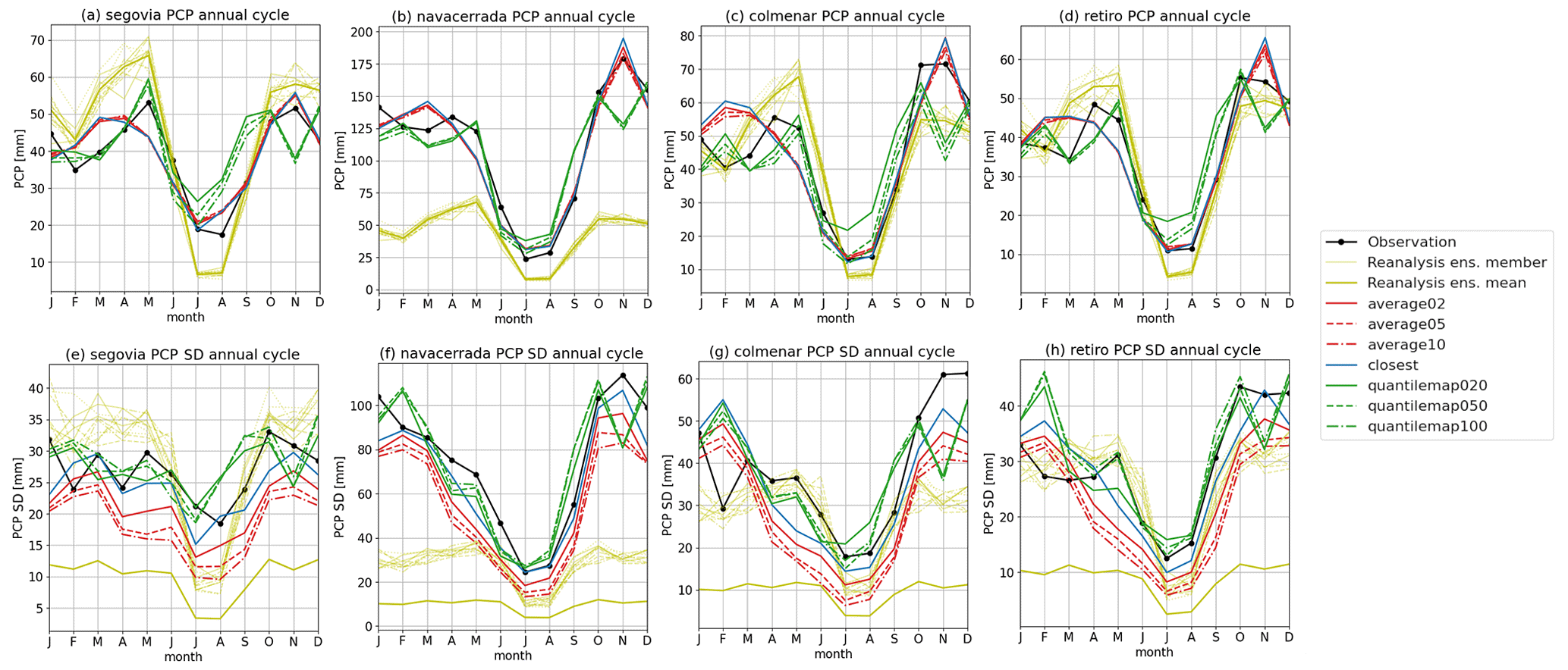
Figure 8 Annual cycle of monthly total precipitation for all the stations (left to right). The first-row panels (a, b, c, d, e) show the cycle for the variable, and the second row (f, g, h, i, j) is for its standard deviation.

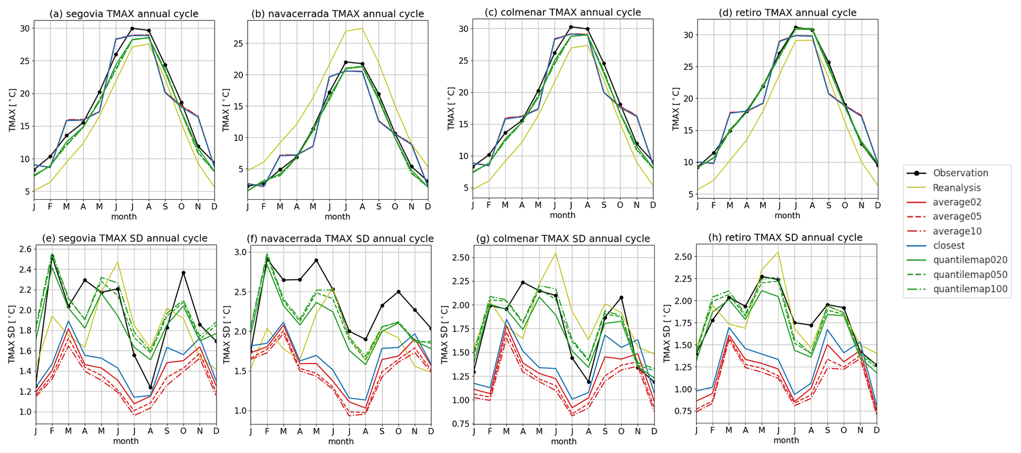
Figure 9 Annual cycle of monthly mean maximum temperature for all the stations (left to right). The first-row panels (a, b, c, d) show the cycle for the variable, and the second row (e, f, g, h) is for its standard deviation.

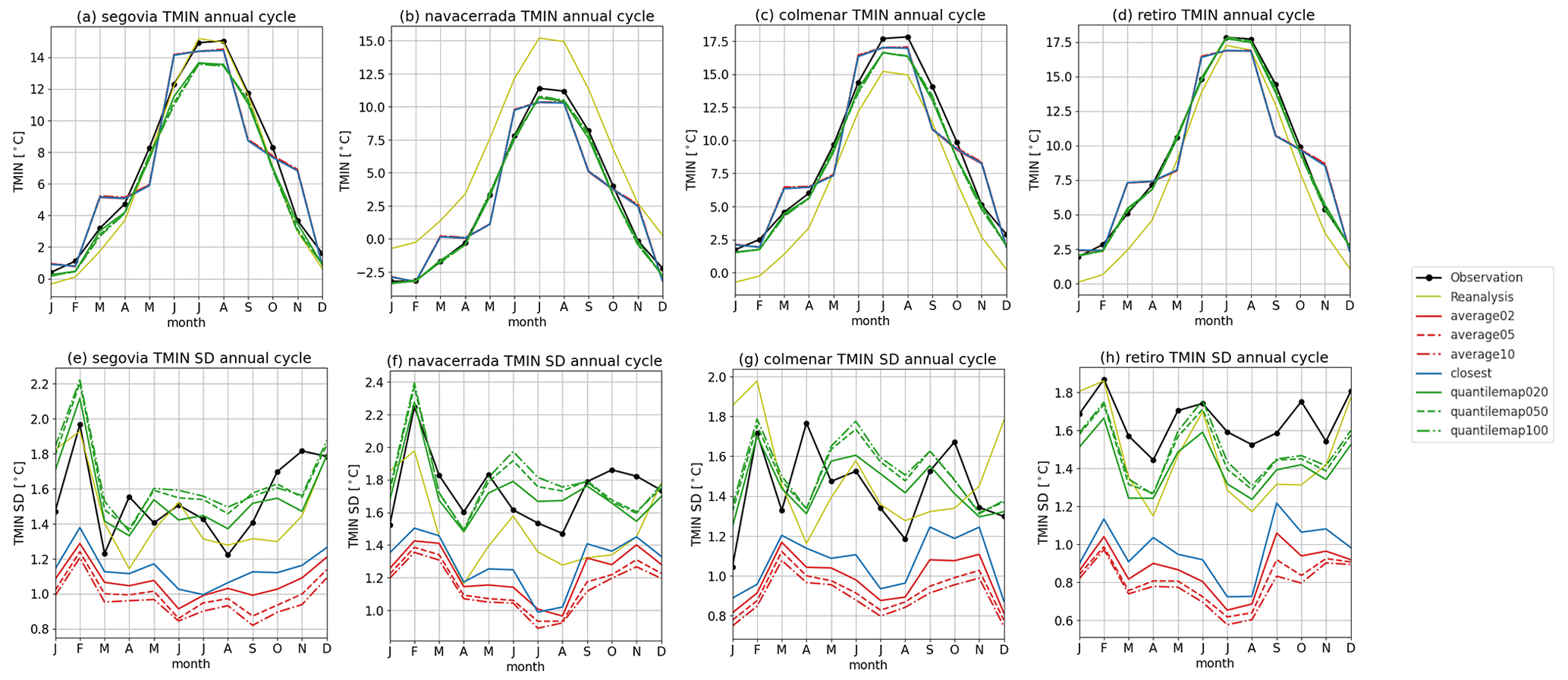
Figure 10 Annual cycle of monthly mean minimum temperature for all the stations (left to right). The first-row panels (a, b, c, d, e) show the cycle for the variable, and the second row (f, g, h, i, j) is for its standard deviation.

4.3.4 Daily indices

In climate studies, it is common to employ indices that condense key climatic features of the study area. These indices are usually based on the comparison of a variable with a fixed threshold or a threshold based on some statistical property, such as a mean value or a percentile (Klein Tank et al., 2009). Consequently, when using climate indices, the focus of a study may not necessarily be on making the reconstructed time series closely resemble the observations, but rather on effectively reproducing these indices. Given that the indices are based on threshold crossings, a dataset characterized by significant biases may result in a misrepresentation of these indices. As demonstrated earlier, the station Navacerrada stands out as the one most positively influenced by the reconstructions. This is due to the fact that the reanalysis provides a deficient representation of precipitation and temperature, mainly due to its pronounced warm and dry bias. Therefore, this station was chosen for the calculation of relevant indices for a mountainous region using the reconstructions, such as days with precipitation exceeding 1 mm (R_1 mm), icing days (IC, days of maximum temperature below 0 °C), and frost days (FD, days of minimum temperature below 0 °C).

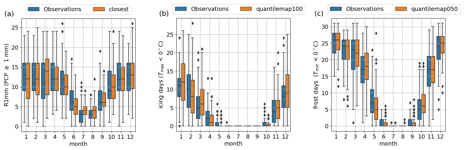
Figure 11 Seasonal cycle of the observations and the best reconstruction of climatological indices in Navacerrada, these being (a) days of PCP ≥ 1 mm (R_1 mm), (b) days of $T_{max}<\mathrm{0}$ °C or icing days (ID), and (c) days of $T_{min}<\mathrm{0}$ °C or frost days (FD).

Table 2 Skill metrics for the best monthly reconstruction in Navacerrada for days of PCP ≥ 1 mm (R_1 mm), icing days (ID), and frost days (FD).

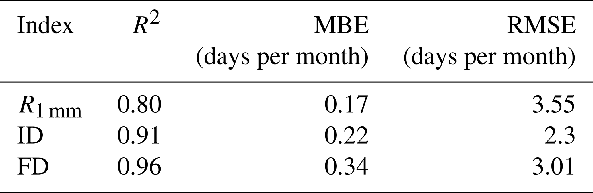
Figure 11 presents the seasonal cycles of the indices for both observations and the optimal reconstruction chosen in Sect. 5.3.1. The aim is to ensure that the reconstructions accurately replicate the climatic characteristics associated with these indices without exhibiting any spurious behavior.

The R_1 mm index in Fig. 11a reveals highly similar distributions across all months, with only a slight overestimation of the median value noted in March, June, and July. Figure 11b also demonstrates very good agreement in the ID index between the reconstruction and observed distributions and median values, although with slightly broader distributions during winter months. Finally, Fig. 11c reaffirms the substantial agreement between observations and distributions for the FD index, highlighting RASCAL's capability to faithfully replicate the seasonal behavior inherent in these indices.

Upon examining the time series skill, Table 2 presents the values for Pearson correlation coefficient (R²), mean bias error (MBE), and root mean square error (RMSE) of the indices. The table highlights the commendable performance of the reconstructions in accurately reproducing these indices, as evidenced by high correlations, particularly for temperature-related indices. Furthermore, the MBE values are significantly low, measuring less than 0.34 d per month, and the RMSE values remain below 3.55 d per month.

5 Conclusions

We have confirmed that a decline of in situ observations is a noteworthy concern as it may result in the loss of crucial information in areas where local effects are relevant to climatology. While the reanalysis provides a homogeneous and comprehensive dataset, its applicability to studying climatologies with highly localized effects, particularly in regions with intricate orography, has been called into question.

In order to mitigate this possible loss of meteorological information based on surface observations, RASCAL has been developed. This is an open-source Python tool designed to fill gaps in observational data, enabling climate studies in regions with limited long-term data. This tool proved to be particularly useful for the test sites, especially in the mountainous areas. It is expected to also be useful in other areas with important local effects or distinctive locations like river valleys, forests, caves, or canyons.

The package presented here utilizes an object-oriented programming (OOP) approach, treating weather stations, predictors, and reconstructions as objects with multiple functional attributes that encompass all necessary functionalities. This has allowed for the execution of all modeling steps with just a few lines of code. The core methodology is based on linking large-scale circulation patterns with local atmospheric features. This linkage is established through the analog method and principal component analysis and has been shown to be more effective than reanalysis in conveying climatic characteristics. It is a faster and less computationally expensive alternative to dynamical downscaling methods and an easier-to-interpret method than machine learning statistical downscaling methods.

The package was evaluated at four stations in Spain, including three near a mountainous area in central Spain and one in a highly urbanized area. The results were compared to the products of the reanalysis ERA20C and ERA20CM. RASCAL outperformed the reanalysis in terms of R², standard deviation, and bias. This improvement was particularly noticeable in the reconstruction of monthly total precipitation, with correlation values reaching 0.8. The reconstructed maximum and minimum temperatures show a slight improvement over the reanalysis in terms of standard deviation and correlation, reaching very high values of correlation of over 0.99. Additionally, the biases present in the reanalysis are significantly corrected by the reconstructions. This is also evident when examining the distributions of daily data. RASCAL is proficient at generating series that closely resemble the observations, unlike the reanalysis, which exhibits skewness towards low precipitation and biases in maximum and minimum temperatures.

The various methods for selecting the best analog have exhibited diverse behaviors when examining the different characteristics of the series. Therefore, it is recommended not to designate a single method as the best possible but to choose it based on the scientific objectives.

Seasonality also demonstrates a marked enhancement compared to the reanalysis. RASCAL produces reconstructions with an annual cycle closely resembling the observations. While the precipitation annual cycle exhibits some disparities during unstable months, such as November and March, the cycles of maximum and minimum temperatures are nearly identical to the observations in every month when using the quantile map method. This method better represents the monthly variability for both precipitation and temperatures.

In climate studies, the use of indices is a common practice to condense key climatic features of a study area. RASCAL has demonstrated its capacity to reproduce indices like days of precipitation above 1 mm, icing days, and frost days well for a station situated in the core of a mountain range. This achievement is particularly noteworthy given the difficult conditions posed by the strong dry and warm biases of the reanalysis in this region, which would otherwise hinder the accurate computation of these indices. The reconstructed data showcase high correlation coefficients with observations, ranging from 0.8 to 0.96. Additionally, consistently low values of MBE and RMSE were observed. These outcomes highlight the significant potential of RASCAL to facilitate climate studies in regions with complex climatic dynamics. These results confirm RASCAL's effectiveness in capturing and reproducing important climatic features for reliable climate research, highlighting its potential in regions with limited long-term weather data.

However, it is important to acknowledge instances where this methodology may have limitations. This approach requires sufficiently long series, as it cannot create reconstructions with data that have not been observed. Additionally, land use changes or urbanization processes can disrupt the intricate relationship between large and small scales, affecting the relationship between predictor and predictand and, ultimately, the quality of the reconstruction.

The implementation of this package has yielded positive results, providing opportunities to conduct comprehensive climate variability analyses within the study area. In a short time, it is expected that we can use RASCAL in the analysis of the climate variability and climate change in the mountainous area of the Central System (Spain). On the other hand, improvements to be implemented in this methodology will be studied once it has been applied to different cases, scenarios, and regions. Finally, whether this package can be extended as a downscaling tool for short- and medium-term numerical forecast, as well as for seasonal prediction and even climate change scenarios, will be analyzed.