A global–land snow scheme (GLASS) v1.0 for the GFDL Earth System Model: formulation and evaluation at instrumented sites

Snowpacks modulate water storage over extended land regions and at the same time play a central role in the surface albedo feedback, impacting the climate system energy balance. Despite the complexity of snow processes and their importance for both land hydrology and global climate, several state-of-the-art land surface models and Earth System Models still employ relatively simple descriptions of the snowpack dynamics. In this study we present a newly-developed snow scheme tailored to the Geophysical Fluid Dynamics Laboratory (GFDL) land model version 4.1. This new snowpack model, named GLASS (Global LAnd–Snow Scheme), includes a refined and dynamical vertical-layering snow structure that allows us to track the temporal evolution of snow grain properties in each snow layer, while at the same time limiting the model computational expense, as is necessary for a model suited to global-scale climate simulations. In GLASS, the evolution of snow grain size and shape is explicitly resolved, with implications for predicted bulk snow properties, as they directly impact snow depth, snow thermal conductivity, and optical properties. Here we describe the physical processes in GLASS and their implementation, as well as the interactions with other surface processes and the land–atmosphere coupling in the GFDL Earth System Model. The performance of GLASS is tested over 10 experimental sites, where in situ observations allow for a comprehensive model evaluation. We find that when compared to the current GFDL snow model, GLASS improves predictions of seasonal snow water equivalent, primarily as a consequence of improved snow albedo. The simulated soil temperature under the snowpack also improves by about 1.5 K on average across the sites, while a negative bias of about 1 K in snow surface temperature is observed.

1 Introduction

Snow is a fundamental component of the global water and energy balance. Over extended regions on Earth, a significant fraction of the water budget is stored over land as snow, so soil moisture, runoff, and water availability for ecosystems and human communities are directly impacted by changes in snow (Cohen and Rind, 1991; Xu and Dirmeyer, 2013). Snow cover also plays an important role in the energy balance at the surface (Qu and Hall, 2014; Thackeray et al., 2018). Compared to other natural surfaces, snow is characterized by the highest reflectivity in the visible range and by exceptionally low heat conductivity. Because of these properties, snow has been shown to significantly affect near-surface temperatures (Armstrong and Brun, 2008; Betts et al., 2014) and to play a primary role in modulating the warming rate of arctic regions (Stieglitz et al., 2003) and permafrost extent (Burke et al., 2013). Thus, the presence of snow fundamentally alters the near-surface temperature and in turn the energy partitioning between the land surface, subsurface, and atmosphere (Henderson et al., 2018). Numerical simulations of snowpacks are used in many scientific applications, ranging from watershed-scale hydrology and flood forecasting (Nester et al., 2012; Blöschl, 1999) to centuries-long, global simulations of the climate system (Kapnick and Delworth, 2013). Given the profound implications of snow for land–atmosphere interactions over extended regions of the Earth, it is paramount that land surface models adequately describe the coupling between snow and soil, vegetation, and the atmosphere.

Fully understanding the implications of snow for land hydrology and the climate system requires a detailed representation of its physical properties in numerical models. The complexity of snow schemes used in land surface modeling varies greatly and has been previously classified in three complexity levels (Boone and Etchevers, 2001; Vionnet et al., 2012). The first class includes the simplest snow models, which consist of either a single snow layer or a composite snow–soil medium. Traditionally these computationally inexpensive snow models have been employed in numerical weather prediction and global climate models. The second class, intermediate-complexity models, addresses several deficiencies in the former class of models by including at least a coarse vertical discretization of the snowpack and by explicitly modeling the liquid-phase water and variations in snow density. Intermediate-detail snowpack models include the European Centre for Medium Range Weather Forecasts (ECMWF) snow scheme (Dutra et al., 2010; Arduini et al., 2019), the Community Land Model (CLM) 4.5 (Oleson et al., 2013), the Canadian Land Surface Scheme (CLASS), the Joint UK Land Environment Simulator (JULES; Best et al., 2011), Snow17 (Anderson, 1976), and WEB-DHM-S (Shrestha et al., 2010).

Finally, the third class consists of detailed snowpack models: these are characterized by a much-finer vertical layering of the snow, which can evolve dynamically with snowfall and snowmelt. Snow microphysical properties are tracked in each snow layer, thus allowing for a more realistic description of physical processes. Such highly detailed snowpack models include SNOWPACK (Bartelt and Lehning, 2002; Lehning et al., 2002b, a), SNTHERM89 (Jordan, 1991), and CROCUS (Brun et al., 1992, 1997; Vionnet et al., 2012). Some models explicitly resolve the propagation of shortwave radiation within the snow layers, for example, the Snow, Ice, and Aerosol Radiative Model (SNICAR; Flanner and Zender, 2005, and Flanner et al., 2007); the Two-stream Analytical Radiative TransfEr in Snow (TARTES; Libois et al., 2013); and Glacier Energy and Mass Balance (GEMB; Gardner et al., 2023). Since higher-detail snow schemes tend to be computationally expensive, applications of snow models targeting long, global-scale numerical simulations of the Earth system must strike a balance between physical detail and computational demands. Despite the need for this tradeoff, it has been recognized that a number of physical processes impacting the evolution of the snowpack should be resolved in land surface models, as they can be relevant for large-scale hydrological studies and for coupled climate simulations. These include the effect of thermal insulation (Cook et al., 2008; Lawrence and Slater, 2010) and the effect of snow microphysics on albedo (Flanner and Zender, 2006; Vionnet et al., 2012; He et al., 2017).

The increasing fidelity of snow processes using detailed snow schemes has been shown to benefit both climate studies (Dutra et al., 2010; Decharme et al., 2016) and numerical weather prediction applications (Arduini et al., 2019), as snow not only impacts the hydrological response but also interacts with the atmosphere through surface temperature and reflectivity.

The snow scheme currently implemented in the Geophysical Fluid Dynamics Laboratory (GFDL) land model (LM) 4.1 (Shevliakova et al., 2024) can be considered a scheme of intermediate complexity: the snowpack is characterized by a fixed number of vertical layers (routinely set to five), each characterized by its temperature and ice and liquid-water content. However, the density of the snow is set to a constant value (currently, 250 kg m⁻³), so the model provides limited information on snow depth. As a consequence, snow heat conductance is also a constant, which can lead to challenges in determining the vertical temperature profile of snow and soil. Finally, no description of snow microphysics is present, so the dependence of physical processes on the snow microstructure (e.g., the evolution of snow optical properties with age and snow compaction) is not accounted for. However, this parsimonious snowpack model has been successfully employed to simulate snow cover at the global scale (Kapnick and Delworth, 2013).

The focus of this work is to present the Global LAnd Snow Scheme (GLASS), a novel snow model developed for LM 4.1. The primary objective of the development of GLASS is to increase the realism of the snow processes in LM 4.1, while at the same time limiting the computational burden of the model so that it can be effectively employed in global Earth system simulations. Key physical processes that were absent in LM 4.1 have been adapted in GLASS from existing parameterizations used in detailed snow schemes. In particular, GLASS now includes the treatment of snow compaction, wind drift effect, and snow aging and accounts for the effects of these processes on snow thermal and optical properties. The evolution of snow properties with snow aging accounts for both dry and wet metamorphism. In GLASS these processes affect not only the growth of snow grains but also the evolution of their shape. This information is in turn employed to evaluate snow albedo, which in GLASS depends explicitly on both the optical size and optical shape of snow grains. While increasing the fidelity of the snow physical processes, GLASS builds on the existing implicit solution scheme for the fluxes between land and atmosphere, which is numerically stable and efficient for the time step (30 min) routinely used in global-scale coupled land–atmosphere simulations. To avoid an excessive increase in the computational demands of the new snow model, the energy balance at the land surface is linearized in LM 4.1. This approach leads to a tradeoff between computational cost and physical realism, as an iterative solution of the energy balance would lead to a considerable increase in computational expense. GLASS is characterized by a dynamic snow vertical-layering structure that allows the efficient tracking of the evolution of snow properties with age, as is currently done by a few high-detail snow schemes such as CROCUS (Brun et al., 1992; Vionnet et al., 2012). A re-layering scheme is used to determine the optimal vertical discretization of the snowpack so as to obtain a proper tradeoff between model detail and computational expense.

After presenting the features of GLASS, we test its performance over a set of sites widely used as benchmark, including in previous snow model intercomparison efforts (Krinner et al., 2018). The dataset used here spans a wide range of climate and terrain conditions so as to characterize the behavior of the model. The evolution of snowpack in vegetated areas constitutes a major source of uncertainty, which carries potentially large implications for constraining the snow albedo feedback over the Northern Hemisphere. We contribute to this challenge by evaluating GLASS at three forested sites that are part of the ESM-SnowMIP project. The remainder of the paper is organized as follows: Sect. 2 describes in detail the model physics and implementation in LM 4.1, including the existing treatment of snow processes. GLASS is presented in detail in Sect. 3. Section 4 describes the experimental setup used in our study as well as the data used as model input and atmospheric forcing and the snow data used for model validation. Results and discussion follow in Sects. 5 and 6, while model limitations and considerations for future research directions are discussed in Sect. 6. Conclusions from this study are featured in Sect. 7.

2 Overview of land and snow processes represented in the GFDL land model

2.1 Land model overview

The land component of GFDL ESM 4.1 (Dunne et al., 2020; Shevliakova et al., 2024), hereafter called LM 4.1, provides a detailed description of the key processes involved in the mass and energy exchanges between land and atmosphere. In LM 4.1, the land domain is discretized in a number of grid cells. To represent the effects of heterogeneity of land–atmosphere interactions and terrestrial biogeochemical processes, the model employs a mosaic approach where each grid cell can be further split into a set of sub-grid tiles: fractions of the grid cell with distinct physical and biogeochemical properties. LM 4.1 resolves the land–atmosphere exchanges of energy, water, and tracers separately for each of the tiles. The evolution of the relevant terrestrial properties – the state of vegetation, albedo, soil moisture and temperature, snow cover, etc. – is also simulated separately for each of the tiles, while allowing for interaction due to land use transitions and other processes that can dynamically change the tiling structure. Such an approach captures the effects that land use has on land–atmosphere physical interactions, as well as on the terrestrial carbon cycle (Shevliakova et al., 2009; Malyshev et al., 2015; Chaney et al., 2018; Zorzetto et al., 2023). Vegetation in the model is dynamic, represented by a set of cohorts with each cohort being a set of plants with similar characteristics, i.e., species, size, and age. Cohorts change as the vegetation assimilates carbon (and undergoes other processes such as mortality and reproduction) and organize themselves in a number of layers, according to the perfect plasticity approximation (PPA) approach (Strigul et al., 2008; Weng et al., 2015; Martínez Cano et al., 2020). In the present application, we employ a configuration of the model where we focus on a single tile that corresponds to each of the sites where point-scale observations were obtained. The time step used in the model for physical processes related to snow, soil, and land–atmosphere interactions is 30 min. In GFDL LM 4.1, the sensible heat (H_g) and evaporation (E_g) fluxes are computed using the bulk formulae driven by the gradient in temperature and specific humidity between atmosphere (T_a, q_a) and the near-surface canopy air layer (T_c, q_c),

$$\begin{array}{}\text{(1)}& {\displaystyle }{H}_{\mathrm{g}}={\mathit{\rho }}_{\text{air}}{c}_p{C}_{\mathrm{D}}\stackrel{\mathrm{‾}}{U}(T_{\mathrm{c}}-T_{\mathrm{a}})\text{(2)}& {\displaystyle }{E}_{\mathrm{g}}={\mathit{\rho }}_{\text{air}}{C}_{\mathrm{D}}\stackrel{\mathrm{‾}}{U}(q_{\mathrm{c}}-q_{\mathrm{a}}),\end{array}$$

where $\stackrel{\mathrm{‾}}{U}$ is the wind above the constant flux layer and C_D is the stability-dependent drag coefficient computed from the Monin–Obukhov similarity theory (Garratt, 1994; Foken and Napo, 2008), c_p is the specific heat of air, and ρ_air is the air density. Within the vegetation canopy, the aerodynamic resistance is computed assuming an exponential wind velocity profile following the approach by Bonan (1996). In the present work, we use the same formulation for turbulent fluxes in all model configurations described below.

2.2 Snow scheme in LM 4.1

The existing snow module part of GFDL LM 4.1 (named current model, LM-CM, or CM throughout this work) can be classified as an intermediate-complexity snow scheme according to the definition by Boone and Etchevers (2001). Fluxes of water and heat in the snowpack and soil continuum are based on the model by Milly et al. (2014). If snow is present on the ground, the snowpack is composed of a fixed number of levels, routinely set to five. Each snow layer is characterized by its temperature and by its liquid and ice mass content. No description of snow microphysics is present, so key snow properties (in particular, snow density and heat conductance) are assumed to be constant. Light does not penetrate the snowpack: shortwave radiation contributes to the surface energy balance, and the resulting net heat flux constitutes the upper-boundary condition for resolving the heat diffusion through the snow layers and the underlying soil. The snow albedo is computed with an empirical formulation based on the bidirectional reflectance distribution function (BRDF) described in Appendix C. This model does not explicitly account for the effects of snow grain size or for the presence of light absorbing particles within the snow but rather yields typical reflectivity values for snow-covered surfaces. The effect of snow metamorphism on its optical properties is mimicked by introducing a dependence of the BRDF model parameters on the temperature of the uppermost snow layer, with warm snow being characterized by reduced reflectivity.

3 The Global LAnd–Snow Scheme (GLASS) in LM 4.1

GLASS was developed building upon the existing LM-CM snow scheme with the objective of including representations of important snow physical processes in the model. For each LM 4.1 model tile, GLASS is a 1D snow model coupled to the soil and multilayer canopy scheme parts of LM 4.1. GLASS simulates the evolution of the snowpack and the exchanges of water and energy with the lower atmosphere and the underlying soil. The vertical discretization of the snowpack is dynamic, with the number and thickness of snow layers being determined by both history (e.g., new snow layers being added on top of the snowpack due to precipitation events) and computational considerations, so snow layers can split and merge, tending toward an optimal vertical profile. In GLASS, each snow horizontal layer is characterized by a number of physical properties. A schematic representation of the snow vertical structure in GLASS is shown in Fig. 1. Energy and mass fluxes at the upper boundary of this medium are determined by liquid and solid precipitation (possibly percolating through canopy layers if vegetation is present), evaporation, or sublimation, and the net heat flux into or out of the snowpack is determined by solving the energy balance at the surface. Shortwave radiation can penetrate the snowpack depending on its thickness and optical properties, as discussed below. At the bottom of the snow column, the boundary condition is given by the flux of heat and water into the underlying soil layers or by runoff.

Figure 1 A schematic representation of the fluxes of energy and water included in the GLASS snow model. The dashed red and green rectangles indicate the energy flux terms contributing to the surface energy balance and the shortwave radiative balance at the surface, respectively. Exchange terms include net longwave (R_Lg) and net shortwave (R_Sg) radiation (with downward and upward radiation denoted by R_Sd and R_Su, respectively), as well as sensible heat flux (H_g), latent heat of sublimation (L_gE_g), and the melting rate at the ground (M_g). Solid (f_s) and liquid (f_l) precipitation rates are also represented. Heat fluxes between layers (H_k) and heat sources due to shortwave radiation absorption (S_k) within the snowpack are also represented, as is the snowpack contribution to runoff (R_sn,l) and liquid-water infiltration into soil (I_sn,l). Fluxes of liquid water (blue arrows) and ice (pink arrows) are also featured, with q_k for liquid flow between the snowpack layers k and k+1. Note that fluxes of heat advected by solid and liquid precipitation, vertical liquid-water flow within the snowpack, infiltration, and runoff are all represented in the model, although for simplicity they are not explicitly represented in this figure.

3.1 Representation of snow at the ground and its vertical discretization

A fine vertical discretization of the snowpack is key to resolving the vertical variation in snow physical properties that affects the overall snowpack mass and energy balance. In GLASS, this requirement is met by employing a vertical structure that can change dynamically, designed to strike a tradeoff between the desire for physical detail and the need to limit the computational requirements of a model used for global-scale simulations. The snowpack, if present, is composed of a variable number n_L of horizontal layers, numbered from the top of the snowpack to the bottom ($k=\mathrm{1},\mathrm{\dots },n_{\mathrm{L}}$). Each snow layer is characterized by a set of physical properties that evolve dynamically. These are the layer's liquid (w_l,k) and ice (w_s,k) contents, its thickness Δz_k, temperature T_k, heat capacity c_k, and heat conductance λ_k. In each layer, we assume that ice and liquid-water components of the snowpack have the same bulk temperature, which can thus be determined by a single heat conservation equation. Additionally, the physical properties of snow grains in each layer are described by three prognostic variables: the snow grain dendriticy δ_k, sphericity s_p,k, and optical diameter d_opt,k. Together, these three prognostic variables identify the optical size and shape of snow grains and are used for albedo calculations. A complete description of the physical properties of each snow layer is provided in Table 1.

Table 1 List of physical variables characterizing the kth snow layer.

In GLASS, the thickness of the snow layers is adaptive to the snow depth and the thermal regime within the snowpack. To accurately represent the snow thermal conductivity, the layers are generally thinner in the region of high thermal variability in gradients (e.g., near the surface, which is subject to high-frequency variation in fluxes, or in the vicinity of the soil surface) and thicker in the middle of the snowpack. The number and thickness of layers is dynamic. Snowfall events of large-enough magnitude can lead to the creation of Δn_L new layers on top of existing snow or bare soil. Similarly to (Vionnet et al., 2012), Δn_L is given by

$$\begin{array}{}\text{(3)}& \mathrm{\Delta }{n}_{\mathrm{L}}=max\left[max(\mathrm{3}-n_{\mathrm{L}},\mathrm{1}),min(\mathrm{5},\lceil a_{\text{fall}}\cdot \mathrm{\Delta }{z}_{\text{fall}}\rceil )\right],\end{array}$$

where Δz_fall is the depth of newly fallen snow [m] and a_fall=100 m⁻¹. Equation (3) ensures that after snowfall, the number of snow layers n_L+Δn_L is at least three. The number of newly created layers Δn_L originating from the snow falling in a single time step can be up to five, depending on the magnitude of the precipitation event. In the case of a weak precipitation event, instead of creating new layers according to Eq. (3), the precipitating snow mass is added to the existing snowpack's uppermost layer, if any (this happens if the newly deposited snow depth is up to half the depth of the uppermost existing snow layer). In this case, we denote the part of the solid precipitation rate f_s that contributes to the existing top snow layer $f_{{\mathrm{s}}_{\mathrm{1}}}$ so that $f_{{\mathrm{s}}_{\mathrm{1}}}=f_{\mathrm{s}}$ in the case of weak snowfall that does not lead to the creation of new snow layers and $f_{{\mathrm{s}}_{\mathrm{1}}}=\mathrm{0}$ otherwise. In addition to snowfall, other physical processes (e.g., sublimation, snow compaction, and snowmelt) can modify the thickness of existing snow layers. To avoid dealing with a snowpack composed of an excessive number of thin layers, GLASS performs a re-layering of the snowpack at each time step, with the objective of avoiding excessive costs in computation time and memory as well as potential numerical instabilities originating from dealing with very small snow layers resulting from snowmelt or sublimation.

The model optimizes the vertical layering of the snowpack by comparing the current layers with an optimal vertical distribution of snow layers defined for the current snow depth value. The optimal distribution of layers is designed with the objective of maintaining relatively thin layers close to the surface, in order to better resolve heat diffusion and snowpack properties, and coarser layers at depth so as to limit the overall number of layers. This is achieved by first specifying the optimal thickness of the top and bottom layers. Below the first specified top layer, the optimal layers increase in thickness with a given constant ratio (set to 1.5 in the current model configuration) until they reach a specified maximum thickness (1 m in the default configuration used here). These parameter values were selected in order to restrain the number of layers for computing efficiency, while allowing for relatively thin layers close to the surface so as to better represent the vertical heterogeneity of snow properties and the temperature gradient close to the snow surface. There is no maximum number of snow layers set in the model.

At each model time step, the current snowpack vertical structure is compared with the optimal one, and differences are minimized through merging and splitting of existing snow layers. To merge or split the layer k, GLASS examines a penalty function 𝒫_ℒ that, given boundaries of the layers z_k, k=0…n_L, returns a value indicating how far the current distribution is from the optimal configuration:

$$\begin{array}{}\text{(4)}& {\mathcal{P}}_{\mathcal{L}}=\sum _{i=\mathrm{0}}^{n_{\mathrm{L}}-\mathrm{1}}{\left(z_{i+\mathrm{1}}-z_i-{\mathcal{D}}_{\mathcal{L}}\left(z_i\right)\right)}^{\mathrm{2}},\end{array}$$

where 𝒟_ℒ(z) is the optimal layer thickness at depth z given the current snow depth. The model loops through the existing snow layers and for each layer compares the current value of 𝒫_ℒ with the corresponding metric evaluated after merging the current layer with the next. If after the merging of the layers the new value of the error metric is lower, the two layers are merged, unless the layers are not otherwise prohibited from merging because they have significantly different physical properties. Similarly, in a second loop GLASS attempts to split each layer by comparing the metric 𝒫_ℒ with that relative to a new profile obtained by splitting a layer in two. Any time this comparison leads to a decrease in the metric 𝒫_ℒ, the layer is split in two before examining the next. Two layers can be merged only if their physical properties are not too dissimilar. In the current application, we allow the merging of layers k and k+1 only if their differences in grain sphericity, optical diameter, and snow density are below given thresholds (namely, $|s_{\mathrm{p},k}-s_{\mathrm{p},k+\mathrm{1}}|<\mathrm{0.2}$, $|d_{\text{opt},k}-d_{\text{opt},k+\mathrm{1}}|<\mathrm{1}\times {\mathrm{10}}^{-\mathrm{4}}$ m, and $|{\mathit{\rho }}_k-{\mathit{\rho }}_{k+\mathrm{1}}|<\mathrm{30}$ kg m⁻³). Thus, in the process of merging snow layers for computational purposes, the vertical heterogeneity of snow physical properties is taken into account and is preserved to some extent. At each time step, the vertical-layering profile of the snow is compared to this theoretical optimal profile. The distance of each layer from the optical thickness at that depth is compared to that of the profiles obtained from splitting and merging each layer with its neighbors. If such operations lead to a vertical profile that is closer to the optimal one, the split or merge operation is performed on the snow layers. While there is no upper limit on the number of layers, this approach allows us to control the evolution of the snow vertical profile.

3.2 Energy balance at the surface

Figure 1 provides a schematic representation of the physical processes included in the snow model. The energy balance at the surface is coupled with that of the snow or soil underneath and the vegetation layers and canopy air above, and it can be expressed [W m⁻²] as

$$\begin{array}{}\text{(5)}& R_{\text{sg}}^{*}+R_{\text{lg}}-H_{\mathrm{g}}-L_{\mathrm{g}}{E}_{\mathrm{g}}-G-L_{\mathrm{f}}{M}_{\mathrm{g}}=\mathrm{0},\end{array}$$

where R_lg is the longwave net radiative flux at the surface, L_f is the latent heat of water fusion, L_g the latent heat of evaporation or sublimation, E_g the rate of evaporation or sublimation, G the heat flux into or out of the ground, and M_g the melting rate of water at the surface (if >0, otherwise it is the freezing rate). In the presence of deep-enough snowpacks (snow depth $h_{\mathrm{s}}>h_{\text{sw},\text{min}}=\mathrm{0.02}$ m by default), the net shortwave radiation R_sg is absorbed within the snowpack instead of contributing to the surface energy balance and thus $R_{\text{sg}}^{*}=\mathrm{0}$. In the case of thinner snowpacks, $R_{\text{sg}}^{*}=R_{\text{sg}}$. Similarly, the latent heat carried by precipitation is accounted for in the energy balance of the underlying snowpack or soil where precipitation accumulates. Equation (5) is solved together with the equations of mass and energy balance of canopy air, the energy balance of any vegetation canopy layers, and the mass balance of any liquid or solid water intercepted by canopy layers.

In order to run efficiently in long, global-scale simulations, the solution of this system of equations must avoid excessive computational costs and be numerically stable for relatively large time steps (the present application uses a 30 min time step, which corresponds to the physics time step in a typical GFDL atmospheric model configuration). To avoid numerical instabilities, the system is solved using a fully implicit scheme. This is done by linearizing the system of equations around the current value of its prognostic variables. These are the temperatures of the ground, vegetation canopies, and canopy air; mass of liquid or frozen water intercepted by the canopies; and the specific humidity of canopy air. The solution of this system of equations conserves energy and water mass as required by long Earth-system simulations. However, the rate M_g of water melting or freezing at the surface of the snowpack (if present) or at the ground surface (if snow is absent) imposes a significant non-linearity on Eq. (5) since this term is constrained by the amount of liquid or frozen water that can undergo phase change in the snowpack or in the upper soil layer. In this case, following the procedure by Milly et al. (2014), the single nonlinear Eq. (5) is solved in order to obtain the change in temperature at the surface of the ground (or if the snowpack is present, the temperature at the top of the snowpack), T_g, which in turn is used to obtain the tendencies of all other prognostic variables of the problem from the linearized system. The solution of Eq. (5) uses the current liquid or solid mass available (in the snowpack if present or in the uppermost soil level otherwise) to provide a constraint for the change in phase rate M_g. The new temperature T_g+ΔT_g obtained by the solution of Eq. (5) will then be propagated downward through the snowpack by solving the vertical heat diffusion process implicitly.

3.3 Snowpack mass balance

In GLASS, the evolution of the snowpack is computed by solving the energy and mass conservation equations for each snow layer. The model representation of all physical processes is energy and mass conserving, as required for century-long simulations. The mass balance of total (liquid and frozen) water for the entire snowpack reads

$$\begin{array}{}\text{(6)}& {\displaystyle \frac{\mathrm{d}{W}_{\text{sn}}}{\mathrm{d}t}}=f_{\mathrm{l}}+f_{\mathrm{s}}-E_{\mathrm{g}}-I_{\text{sn},\mathrm{l}}-R_{\text{sn},\mathrm{l}},\end{array}$$

where $W_{\text{sn}}=W_{\text{sn},\mathrm{l}}+W_{\text{sn},\mathrm{s}}$ [kg m⁻²] is the total water content of the snowpack (i.e., the snow water equivalent), with $W_{\text{sn},\mathrm{s}}={\sum }_{k=\mathrm{1}}^{n_{\mathrm{L}}}{w}_{\mathrm{s},k}$ and $W_{\text{sn},\mathrm{l}}={\sum }_{k=\mathrm{1}}^{n_{\mathrm{L}}}{w}_{\mathrm{l},k}$. The flux terms on the right-hand side of Eq. (6) [$\mathrm{kg}{\mathrm{m}}^{-\mathrm{2}}{\mathrm{s}}^{-\mathrm{1}}$] represent the liquid (f_l) and solid (f_s) effective precipitation rates (i.e., net of any canopy interception), the snow sublimation rate (E_g), the liquid-water flux to the underlying soil (I_sn,l), and the contribution to the grid cell runoff from the snowpack (R_sn,l). If snow is present on the ground, only sublimation occurs in GLASS. The mass balance in Eq. (6) is solved by adding any new snow layers created by fresh snowfall according to Eq. (3) and by solving the balance of liquid and frozen water for each snow layer. The liquid mass balance for snow layer k reads

$$\begin{array}{}\text{(7)}& {\displaystyle \frac{\mathrm{d}{w}_{\mathrm{l},k}}{\mathrm{d}t}}=q_{\mathrm{l},k-\mathrm{1}}-q_{\mathrm{l},k}+M_k,\end{array}$$

where M_k is the total melt (or freeze) rate in layer k, $q_{\mathrm{l},k-\mathrm{1}}$ is the flow rate from layer k−1 to layer k, and q_l,k is that from layer k to k+1. The boundary conditions for Eq. (7) are q₀=f_l at the top of the snowpack and $q_{n_{\mathrm{L}}}=I_{\text{sn},\mathrm{l}}$ at the bottom of the snowpack. For the solid mass balance in layer k, we have

$$\begin{array}{}\text{(8)}& {\displaystyle \frac{\mathrm{d}{w}_{\mathrm{s},k}}{\mathrm{d}t}}=-M_k+E_{{\mathrm{g}}_k}+f_{{\mathrm{s}}_k},\end{array}$$

where $E_{{\mathrm{g}}_k}=E_{\mathrm{g}}$ if k=1, else $E_{{\mathrm{g}}_k}=\mathrm{0}$, and $f_{{\mathrm{s}}_k}=f_{{\mathrm{s}}_{\mathrm{1}}}$ if k=1, else $f_{{\mathrm{s}}_k}=\mathrm{0}$. Here $f_{{\mathrm{s}}_{\mathrm{1}}}$ is the fraction of effective solid precipitation that does not create new snow layers according to Eq. (3). Note that in GLASS the total snowmelt M_k is computed in two steps: first, when solving the surface energy balance implicitly, an estimate of the total melt is obtained and the corresponding latent energy flux contributes to the energy balance at the snow surface. Then, when solving the vertical water flow and surface energy balance through the snowpack, additional melting or freezing can occur in order to satisfy thermodynamic constraints (i.e., the thermodynamic equilibrium of each layer is computed, which can lead to additional melting or freezing occurring).

3.4 Snowpack energy balance

The vertical energy balance in the snowpack is expressed as

$$\begin{array}{}\text{(9)}& {\displaystyle \frac{\partial H_{\text{sn}}}{\partial t}}={\displaystyle \frac{\partial q_{\mathrm{h}}}{\partial z}}+S_z,\end{array}$$

with H_sn being the energy content of the snow, S_z the local source term due to shortwave radiation absorbed within the snowpack, and q_h the vertical heat flux given by

$$\begin{array}{}\text{(10)}& q_{\mathrm{h}}=-\mathit{\lambda }{\displaystyle \frac{\partial T}{\partial z}}+c_{\mathrm{l}}{q}_{\mathrm{l}}(T_{\mathrm{l}}-T_{\mathrm{F}}),\end{array}$$

where T_l is the temperature of the vertical water flow of rate q_l, T(z) is the local snow temperature and depth z, T_F is the freezing temperature of water, λ is the snow thermal conductivity, and c_l the specific heat of liquid water. The boundary condition at the top of the snow (z=0) is given by the net heat flux at the surface from Eq. (5) and by the effective liquid precipitation rate $q_{\mathrm{l}}{|}_{z=\mathrm{0}}=f_{\mathrm{l}}$ and its temperature $T_{\mathrm{l}}{|}_{z=\mathrm{0}}=T_{\text{pr},\mathrm{l}}$.

The bottom-boundary condition (at z=z_b) between snow and soil reads

$$\begin{array}{}\text{(11)}& {\displaystyle }\begin{array}{rl}{\displaystyle }-\mathit{\lambda }& {\displaystyle }{\left.\left({\displaystyle \frac{\partial T}{\partial z}}\right)\right|}_{z=z_{\mathrm{b}},\text{soil}}\\ {\displaystyle }& {\displaystyle }=\mathit{\lambda }{\left.\left({\displaystyle \frac{\partial T}{\partial z}}\right)\right|}_{z=z_{\mathrm{b}},\text{snow}}+c_{\mathrm{l}}\left(T_{\mathrm{l}}{|}_{z=z_{\mathrm{b}}}-T_{\mathrm{F}}\right)I_{\text{sn},\mathrm{l}}\end{array}\end{array}$$

and additionally $T{|}_{z=z_{\mathrm{b}},\text{snow}}=T{|}_{z=z_{\mathrm{b}},\text{soil}}$.

3.5 Numerical solution for the energy balance of the snowpack

Following the approach already used in LM 4.1 (Milly et al., 2014), we solve the energy conservation within the snowpack by separating “dry” processes (heat conduction and sublimation from the top layer) from “wet” processes, i.e., those related to the vertical flux of liquid water. The heat content of a snow layer is defined with respect to ice at freezing temperature – i.e., for snow layer k, the heat content is defined as

$$\begin{array}{}\text{(12)}& H_{\text{sn},k}=(c_{\mathrm{l}}{w}_{\mathrm{l},k}+c_{\mathrm{s}}{w}_{\mathrm{s},k})(T_k-T_{\mathrm{F}})+L_{\mathrm{f}}{w}_{\mathrm{l},k},\end{array}$$

where c_s and c_l are the specific heats of solid and liquid water, respectively [$\mathrm{J}{\mathrm{kg}}^{-\mathrm{1}}{\mathrm{K}}^{-\mathrm{1}}$], and L_f is the latent heat of fusion of water at freezing point [J kg⁻¹]. The vertical heat diffusion equation is solved by discretizing the equation over the vertical layer structure of the snowpack.

For layer k we have

$$\begin{array}{}\text{(13)}& c_k{\displaystyle \frac{\partial T_k}{\partial t}}=H_{k-\mathrm{1}}(T_{k-\mathrm{1}},T_k)-H_k(T_k,T_{k+\mathrm{1}})+S_k,\end{array}$$

where $c_k=c_{\mathrm{l}}{w}_{\mathrm{l},k}+c_{\mathrm{s}}{w}_{\mathrm{s},k}$, H_k is the downward heat flux through the bottom of the layer k to layer k+1, and S_k represents the heat source term in layer k from the absorption of solar radiation. We linearize fluxes around their values at the beginning of the time step:

$$\begin{array}{}\text{(14)}& {\displaystyle }\begin{array}{rl}{\displaystyle }{H}_k& {\displaystyle }=H_{\mathrm{0},k}+{\displaystyle \frac{\partial H_k}{\partial T_k}}\mathrm{\Delta }{T}_k+{\displaystyle \frac{\partial H_k}{\partial T_{k+\mathrm{1}}}}\mathrm{\Delta }{T}_{k+\mathrm{1}}\\ {\displaystyle }& {\displaystyle }=H_{\mathrm{0},k}+{\mathrm{\Lambda }}_k\mathrm{\Delta }{T}_k-{\mathrm{\Lambda }}_k\mathrm{\Delta }{T}_{k+\mathrm{1}},\end{array}\end{array}$$

where Λ_k is the heat conductance between the snow layers, defined next.

3.6 Heat conductance between snow layers

For two consecutive snow layers, k and k+1, each with its own thickness (Δz_k) and heat conductivity (λ_k), the resistance to the downward heat flux between layers can be expressed as

$$\begin{array}{}\text{(15)}& {\displaystyle \frac{\mathrm{1}}{{\mathrm{\Lambda }}_k}}={\displaystyle \frac{\mathrm{\Delta }{z}_k}{\mathrm{2}{\mathit{\lambda }}_k}}+{\displaystyle \frac{\mathrm{\Delta }{z}_{k+\mathrm{1}}}{\mathrm{2}{\mathit{\lambda }}_{k+\mathrm{1}}}}={\displaystyle \frac{\mathrm{1}}{\mathrm{2}}}{\displaystyle \frac{{\mathit{\lambda }}_k\mathrm{\Delta }{z}_{k+\mathrm{1}}+{\mathit{\lambda }}_{k+\mathrm{1}}\mathrm{\Delta }{z}_k}{{\mathit{\lambda }}_k{\mathit{\lambda }}_{k+\mathrm{1}}}}.\end{array}$$

The downward heat flux from layer k to k+1 is therefore $H_k={\mathrm{\Lambda }}_k(T_k-T_{k+\mathrm{1}})$. The thermal conductivity of the snowpack λ_k [$\mathrm{W}{\mathrm{m}}^{-\mathrm{1}}{\mathrm{K}}^{-\mathrm{1}}$] is parameterized as a function of snow density ρ_k in each layer [kg m⁻³] using the parameterization proposed by Calonne et al. (2011) and Sun et al. (1999) and used, e.g., in Arduini et al. (2019). In this formulation, the total snow thermal conductivity is the sum of two terms. The first is a quadratic function of density representing the actual snow thermal conductivity (Calonne et al., 2011), while a second term accounts for the additional heat advected by water vapor (Sun et al., 1999):

$$\begin{array}{}\text{(16)}& {\displaystyle }\begin{array}{rl}{\displaystyle }{\mathit{\lambda }}_k& {\displaystyle }={\mathit{\lambda }}_{\mathrm{c},k}+{\mathit{\lambda }}_{\text{wv},k}\\ {\displaystyle }& {\displaystyle }=(a_{\mathrm{1}}{\mathit{\rho }}_k^{\mathrm{2}}-a_{\mathrm{2}}{\mathit{\rho }}_k+a_{\mathrm{3}})+{\displaystyle \frac{P_{\mathrm{0}}}{P_{\mathrm{a}}}}\left(b_{\mathrm{1}}-{\displaystyle \frac{b_{\mathrm{2}}}{T_k-b_{\mathrm{3}}}}\right),\end{array}\end{array}$$

where $a_{\mathrm{1}}=\mathrm{2.5}\times {\mathrm{10}}^{-\mathrm{6}}$ $\mathrm{W}{\mathrm{m}}^{\mathrm{5}}{\mathrm{K}}^{-\mathrm{1}}{\mathrm{kg}}^{-\mathrm{2}}$, $a_{\mathrm{2}}=\mathrm{1.23}\times {\mathrm{10}}^{-\mathrm{4}}$ $\mathrm{W}{\mathrm{m}}^{\mathrm{2}}{\mathrm{K}}^{-\mathrm{1}}{\mathrm{kg}}^{-\mathrm{1}}$, a₃=0.024 $\mathrm{W}{\mathrm{m}}^{-\mathrm{1}}{\mathrm{K}}^{-\mathrm{1}}$, $b_{\mathrm{1}}=-\mathrm{0.06023}$ $\mathrm{W}{\mathrm{m}}^{-\mathrm{1}}{\mathrm{K}}^{-\mathrm{1}}$, b₂=2.5425 W m⁻¹, and b₃=289.99 K. P_a is the near-surface atmospheric pressure and P₀=1000 hPa. In this application, we use Eq. (16) for λ_k as it accounts for the effects of water vapor. As an alternative, we also implemented the snow heat conductance formulation proposed by Yen (1981) used, e.g., in Lafaysse et al. (2017). In this case the effective snow heat conductance is expressed as

$$\begin{array}{}\text{(17)}& {\mathit{\lambda }}_k=max\left\{a_{\mathit{\lambda }}{\left({\displaystyle \frac{{\mathit{\rho }}_k}{{\mathit{\rho }}_{\mathrm{w}}}}\right)}^{\mathrm{1.88}};{\mathit{\lambda }}_{min}\right\},\end{array}$$

with a_λ=2.22 ($\mathrm{W}{\mathrm{m}}^{-\mathrm{1}}{\mathrm{K}}^{-\mathrm{1}}$) and ${\mathit{\lambda }}_{\text{min}}=\mathrm{4}\times {\mathrm{10}}^{-\mathrm{2}}$ ($\mathrm{W}{\mathrm{m}}^{-\mathrm{1}}{\mathrm{K}}^{-\mathrm{1}}$), which are made to match the pure ice heat conductance λ_i with an appropriate choice of a_λ.

3.7 Snow sublimation

The rate of sublimation is computed by solving the nonlinear equation for the surface energy balance, Eq. (5). In the case where a snowpack is present, we assume that the entire water vapor flux comes from sublimation, even if liquid water is present in the snowpack. While this is a simplified assumption, we note that the amount of liquid water present in the snow layers is limited, as we will discuss in Sect. 3.10. The sublimating ice is lost from the uppermost snow layer. In the model, the heat diffusion through the snowpack and sublimation are resolved separately in two consecutive steps. However, since in reality the two phenomena occur simultaneously, the change in heat content of the top snow layer associated with sublimating snow must account for the simultaneous change in the layer's temperature due to vertical diffusion of heat. Therefore, this nonlinear interaction between heat diffusion and heat flux due to sublimating snow is accounted for in GLASS by correcting the layer's temperature to ensure that energy is conserved when both processes are considered as occurring simultaneously. The change in the snowpack energy content is given by two contributions due to mass lost from the uppermost layer and by its change in temperature due to vertical heat diffusion. Due to the implicit numerical scheme used, evaporation and sublimation are linearized around the current temperature value, and their value depends on the surface temperature tendency. To ensure energy conservation, a temperature correction Δ^*ET₁ must be applied to the uppermost snowpack layer since evaporation is computed before the temperature is updated for the current model time step. This is given by

$$\begin{array}{}\text{(18)}& {\displaystyle }\begin{array}{rl}{\displaystyle }& {\displaystyle }[c_{\mathrm{l}}{w}_{\mathrm{l},\mathrm{1}}+c_{\mathrm{s}}(w_{\mathrm{s},\mathrm{1}}+\mathrm{\Delta }{w}_{\mathrm{s},\mathrm{1}}\left)\right](T_{\mathrm{1}}+\mathrm{\Delta }{T}_{\mathrm{1}}+{\mathrm{\Delta }}^{*E}{T}_{\mathrm{1}})\\ {\displaystyle }& {\displaystyle }\begin{array}{rl}{\displaystyle }-(c_{\mathrm{l}}{w}_{\mathrm{l},\mathrm{1}}& {\displaystyle }+c_{\mathrm{s}}{w}_{\mathrm{s},\mathrm{1}})T_{\mathrm{1}}=\\ {\displaystyle }& {\displaystyle }(c_{\mathrm{l}}{w}_{\mathrm{l},\mathrm{1}}+c_{\mathrm{s}}{w}_{\mathrm{s},\mathrm{1}})\mathrm{\Delta }{T}_{\mathrm{1}}+c_{\mathrm{s}}\mathrm{\Delta }{w}_{\mathrm{s},\mathrm{1}}{T}_{\mathrm{1}},\end{array}\end{array}\end{array}$$

where the left-hand side is the change in energy content of the uppermost snow layer, and the two terms on the right-hand side are the change in energy content of the layer due to temperature vertical diffusion and due to sublimation. In Eq. (18), ΔT₁ is the change in temperature in the top snow layer obtained by solving the vertical heat conduction equation, and $\mathrm{\Delta }{w}_{\mathrm{s},\mathrm{1}}=E_{\mathrm{g}}\mathrm{\Delta }t$ is the change in mass of the top snow layer due to sublimation. From Eq. (18) we can solve for Δ^*ET₁:

$$\begin{array}{}\text{(19)}& {\mathrm{\Delta }}^{*E}{T}_{\mathrm{1}}={\displaystyle \frac{c_{\mathrm{s}}\mathrm{\Delta }{w}_{\mathrm{s},\mathrm{1}}}{c_{\mathrm{l}}{w}_{\mathrm{l},\mathrm{1}}+c_{\mathrm{s}}(w_{\mathrm{s},\mathrm{1}}+\mathrm{\Delta }{w}_{\mathrm{s},\mathrm{1}})}}\mathrm{\Delta }{T}_{\mathrm{1}}.\end{array}$$

3.8 Implicit change in phase

Melting imposes an upper limit on the temperature profile in the snowpack since snow temperature should not exceed the melting point. If the solution of the heat equation produces a temperature higher than the freezing temperature (i.e., T_k>T_F for some snow layer k), then the excess energy required to increase the layer temperature by the amount $\mathrm{\Delta }{T}_{*,k}=T_k-T_{\mathrm{F}}$ is instead used to melt a snow mass equal to

$$\begin{array}{}\text{(20)}& \mathrm{\Delta }{w}_{\mathrm{s},k}=min\left\{w_{\mathrm{s},k},{\displaystyle \frac{(c_{\mathrm{s}}{w}_{\mathrm{s},k}+c_{\mathrm{l}}{w}_{\mathrm{l},k})\mathrm{\Delta }{T}_{*,k}}{L_{\mathrm{f}}}}\right\},\end{array}$$

where L_f=334 J kg⁻¹ is the latent heat of fusion of ice, and the expression in the numerator is the specific heat of layer k. For mass conservation, $\mathrm{\Delta }{w}_{\mathrm{l},k}=-\mathrm{\Delta }{w}_{\mathrm{s},k}$. Therefore, the heat required for the phase change is $F_{\mathrm{m},k}=L_{\mathrm{f}}\mathrm{\Delta }{w}_{\mathrm{s},k}<\mathrm{0}$. The new equilibrium temperature $T_{\mathrm{F}}+\mathrm{\Delta }{T}_k^{\left(u\right)}$ of the snow layer is then computed by evaluating the energy conservation equation for layer k:

$$\begin{array}{ll}{\displaystyle }(c_{\mathrm{s}}& {\displaystyle }{w}_{\mathrm{s},k}+c_{\mathrm{l}}{w}_{\mathrm{l},k})\mathrm{\Delta }{T}_{*,k}+w_{\mathrm{l},k}{L}_{\mathrm{f}}=\\ \text{(21)}& {\displaystyle }& {\displaystyle }\left(c_{\mathrm{s}}\right(w_{\mathrm{s},k}+\mathrm{\Delta }{w}_{\mathrm{s},k})+c_{\mathrm{l}}(w_{\mathrm{l},k}-\mathrm{\Delta }{w}_{\mathrm{s},k}\left)\right)\mathrm{\Delta }{T}_k^{\left(u\right)}{\displaystyle }& {\displaystyle }+(w_{\mathrm{l},k}-\mathrm{\Delta }{w}_{\mathrm{s},k})L_{\mathrm{f}},\end{array}$$

which can be solved for the new snow layer equilibrium temperature. Similarly, in the case of T_k<T_F, if $w_{\mathrm{l},k}>\mathrm{0}$, additional energy is provided to the layer by freezing the available liquid water. Again, the amount of energy is limited by the amount of liquid water available for freezing. The temperature of the meltwater is then T_F, while for ice it is T_k<0. Thus, in the case of freezing we have $\mathrm{\Delta }{T}_k^{\left(u\right)}<\mathrm{0}$ and $F_{\mathrm{m},k}=L_{\mathrm{f}}\mathrm{\Delta }{w}_{\mathrm{l},k}>\mathrm{0}$. In the following, we justify our choice of numerical method to solve the snowmelt. The implicit numerical solution of heat conduction through the snowpack must occur in two steps: first, the heat fluxes through the snow as well as their tendencies are calculated, and only in a second step is the temperature profile updated layer by layer. It is therefore possible that when updating the temperature profile, snow layers that were fully frozen become warmer than freezing, and similarly, snow layers that contain water in liquid phase can experience temperatures below freezing. When this happens, the resulting change in phase is computed according to Eqs. (20) and (21). However, solving the phase change according to this procedure, which in the following we call implicit melt or IM, can be problematic in the presence of large time steps, which can produce appreciable temperature increments within the snowpack. In GLASS we use an alternative approach called explicit melt or EM. When solving the nonlinear surface energy balance for the ground temperature balance, we simultaneously compute an estimate for the melt term (M_g) as discussed in Sect. 3.2. By adopting this approach, when we solve the vertical heat diffusion, the heat fluxes we obtain are already consistent with this tentative melt estimate. In the second heat diffusion step, the vertical temperature profile is again updated as in the case of IM, and similarly, additional changes in phase can occur based on the phase and temperature of the existing snow layers. However, since in this approach the tentative melt M_g has already been evaluated, these additional melting or freezing correction terms are generally smaller, and therefore we expect the numerical solution to be less dependent on the time step. Since Earth system models generally run for relatively large time steps (30 min in our land model), in the following we investigate the behavior of the IM and EM approaches for different time steps in order to test their suitability for our application.

3.9 Snowfall and snowpack solid water balance

In the case of snowfall, if (i) there is already snow on the ground and (ii) the new depth Δz_fall is smaller than a threshold (set to half the depth of the uppermost snow layer before the frozen precipitation event), then the new snow is added to the existing layer and no additional layers are created. The density of fresh snow is used to compute Δz_fall, and this snow depth is added to the thickness of the existing layer, so the resulting density of the merged layer will be a weighted average of the of new and existing snow (note, snow density ρ_k is a derived model variable, and it is computed as $w_{\mathrm{s},k}/\mathrm{\Delta }{z}_k$). If instead there is no initial snow on the ground or if the amount of new snow is larger than the set threshold, a number of fresh snow layers are created as discussed in Sect. 3.1. The properties assigned to the freshly fallen snow are computed following Vionnet et al. (2012): the density ρ_fall of new snow is

$$\begin{array}{}\text{(22)}& {\mathit{\rho }}_{\text{fall}}=a_{\mathit{\rho }}+b_{\mathit{\rho }}(T_{\mathrm{a}}-T_{\mathrm{F}})+c_{\mathit{\rho }}{\stackrel{\mathrm{‾}}{U}}^{\mathrm{1}/\mathrm{2}},\end{array}$$

a three-parameter expression in which fresh-snow density is expressed as a function of the mean wind velocity ($\stackrel{\mathrm{‾}}{U}$) and the atmospheric temperature (T_a), with T_F=273.15 K the freezing point of water. Parameters used in Eq. (22) are a_ρ=109 kg m⁻³, b_ρ=6 $\mathrm{kg}{\mathrm{m}}^{-\mathrm{3}}{\mathrm{K}}^{-\mathrm{1}}$, and c_ρ=26 $\mathrm{kg}{\mathrm{m}}^{-\mathrm{7}/\mathrm{2}}{\mathrm{s}}^{-\mathrm{1}/\mathrm{2}}$, setting a minimum snow density of 50 kg m⁻³. The temperature of the fresh snow is equal to that of precipitation, which in the current model configuration is set equal to the temperature of the lower atmosphere. The optical diameter of fresh snow is set to the constant value of $d_{\text{opt},\text{fall}}={\mathrm{10}}^{-\mathrm{4}}$ [m], as recommended by Carmagnola et al. (2014). The (dimensionless) sphericity of fresh snow is computed as was done by Vionnet et al. (2012):

$$\begin{array}{}\text{(23)}& s_{\text{fall}}=min\left[max\left(\mathrm{0.08}\stackrel{\mathrm{‾}}{U}+\mathrm{0.38},\mathrm{0.5}\right),\mathrm{0.9}\right],\end{array}$$

where $\stackrel{\mathrm{‾}}{U}$ is the mean wind speed [m s⁻¹]. Once the density is known, the newly fallen snow depth can be computed from the snowfall rate as $\mathrm{\Delta }{z}_{\text{fall}}=f_{\mathrm{s}}\cdot \mathrm{\Delta }t/{\mathit{\rho }}_{\text{fall}}$.

3.10 Rainfall and the snowpack liquid balance

After updating the snow temperature profile and performing the solid mass balance, the mass balance for the liquid phase is performed. In this stage, the liquid-water balance is evaluated sequentially for all snow layers from the top of the snowpack down, coupled with energy conservation to determine any changes in water phase and temperature originating from the vertical water flow. For the top layer, liquid precipitation is added to the layer. Then, the new thermal equilibrium of the snow layer is computed, determining the new layer temperature and the new mass of liquid and solid water. Finally, the new solid-phase properties are used to determine the pore space available for liquid water within the ice matrix of the layer. As was done by Vionnet et al. (2012), the maximum water-holding capacity in each layer $W_{\text{liq},\text{max},k}$ is set to

$$\begin{array}{}\text{(24)}& W_{\text{liq},\text{max},k}=\mathrm{0.05}{\mathit{\rho }}_{\mathrm{w}}\mathrm{\Delta }{z}_k\left(\mathrm{1}-{\displaystyle \frac{{\mathit{\rho }}_{\mathrm{s},k}}{{\mathit{\rho }}_{\mathrm{i}}}}\right),\end{array}$$

with ρ_s,k the density of the snow layer (solid phase only), ρ_i=917 kg m⁻³ the density of ice, and ρ_w the density of liquid water.

3.11 Snow metamorphism

The snow microstructure in each snow layer k is characterized by three parameters (the layer index k will be omitted in the rest of this section for simplicity): snow optical diameter d_opt, snow dendricity δ, and snow sphericity s_p. The optical diameter d_opt represents the diameter of a monodisperse set of spheres with the same surface-to-mass ratio, or surface specific area (SSA). SSA can be obtained from d_opt as $\text{SSA}=\mathrm{6}/(d_{\text{opt}}\cdot {\mathit{\rho }}_{\mathrm{i}})$. We choose to use d_opt as a prognostic variable because, as pointed out by Carmagnola et al. (2014), it can be directly used to parameterize snow albedo. However, the optical shape of snow grains can also have significant impact on the optical properties of the medium (He et al., 2017; Robledano et al., 2023). The evolution of snow microphysical properties here is obtained as a combination of the parameterizations proposed by Brun et al. (1992), Carmagnola et al. (2014), and Flanner and Zender (2006). In GLASS, all three snow grain properties (grain dendriticy, grain sphericity, and optical diameter) are prognostic variables.

The parameterization of Flanner and Zender (2006), called F06 in the following, is used to model the effects of dry-snow metamorphism on d_opt. In this formulation, the time evolution of the snow optical diameter is computed as a function of snowpack temperature, vertical temperature gradient, and snow density. A parametric equation is used to predict the rate of change in snow effective radius,

$$\begin{array}{}\text{(25)}& {\displaystyle \frac{\mathrm{d}r}{\mathrm{d}t}}={\left.\left({\displaystyle \frac{\mathrm{d}r}{\mathrm{d}t}}\right)\right|}_{t=\mathrm{0}}{\left({\displaystyle \frac{\mathit{\tau }}{r-r_{\mathrm{0}}+\mathit{\tau }}}\right)}^{\mathrm{1}/\mathit{\kappa }},\end{array}$$

where $\left(\frac{\mathrm{d}r}{\mathrm{d}t}\right){|}_{t=\mathrm{0}}$, τ, and κ are parameters derived from a lookup table (here made available in Zorzetto et al., 2024) as functions of snow density, temperature, and temperature gradient. This parameterization was developed by Flanner and Zender (2006) using a physically based model describing the evolution of snow-specific surface area due to dry aging. The optical diameter of fresh snow is taken to be that corresponding to an SSA of 60 m² kg⁻¹. This equation predicts an effective radius in µm, which is then converted to the optical diameter d_opt [m] used in GLASS. For wet snowpacks, the additional size increase in snow grains due to wet metamorphism is described using the model put forward by Brun et al. (1992), in which grain size evolution is given by

$$\begin{array}{}\text{(26)}& {\displaystyle \frac{\mathrm{d}r}{\mathrm{d}t}}={\displaystyle \frac{{\mathrm{10}}^{\mathrm{18}}{C}_{\mathrm{1}}{\mathit{\theta }}_{\mathrm{B}}^{\mathrm{3}}}{\mathrm{4}\mathit{\pi }{r}_{\mathrm{0}}}},\end{array}$$

where $C_{\mathrm{1}}=\mathrm{4.22}\times {\mathrm{10}}^{-\mathrm{13}}$ and ${\mathit{\theta }}_{\mathrm{B}}=w_{\mathrm{l}}/(w_{\mathrm{s}}+w_{\mathrm{l}})$ is the snow liquid fraction. Brun et al.'s equation here is expressed in terms of snow grain radius [µm], which in our model is then converted to snow optical diameter [m]. In addition to the optical diameter, the snowpack layers are characterized by two additional parameters describing the shape of snow grains: dendricity δ and sphericity s_p. These are both dimensionless quantities ranging from 0 to 1. Fresh-fallen snow is assumed to be in a dendritic state, with a dendricity value decreasing over time due to the combined effects of wind drift and metamorphism. When the dendricity parameter approaches zero, the snow reaches a non-dendritic state. Similarly, s_p=1 indicates perfectly spherical particles and s_p=0 completely non-spherical particles, i.e., faceted snow crystals.

The evolution of s_p and δ due to wet- and dry-snow metamorphism is described according to the model by Brun et al. (1992). In the case of wet-snow metamorphism, we have

$$\begin{array}{}\text{(27)}& {\displaystyle \frac{\mathrm{d}\mathit{\delta }}{\mathrm{d}t}}=-{\displaystyle \frac{\mathrm{1}}{\mathrm{16}}}{\mathit{\theta }}^{\mathrm{3}}\text{(28)}& {\displaystyle \frac{\mathrm{d}{s}_{\mathrm{p}}}{\mathrm{d}t}}={\displaystyle \frac{\mathrm{1}}{\mathrm{16}}}{\mathit{\theta }}^{\mathrm{3}},\end{array}$$

with $\mathit{\theta }=\mathrm{100}\cdot w_{\mathrm{l}}/(w_{\mathrm{l}}+w_{\mathrm{s}})$ the percent liquid fraction. For dry metamorphism, the evolution equations for s_p and δ are, in the case of a mild temperature gradient ($G=|\mathrm{d}T/\mathrm{d}z|\le \mathrm{5}$ K m⁻¹),

$$\begin{array}{}\text{(29)}& {\displaystyle \frac{\mathrm{d}{s}_{\mathrm{p}}}{\mathrm{d}t}}={\mathrm{10}}^{\mathrm{9}}{e}^{-\mathrm{6000}/T}\text{(30)}& {\displaystyle \frac{\mathrm{d}\mathit{\delta }}{\mathrm{d}t}}=-\mathrm{2}\times {\mathrm{10}}^{\mathrm{8}}{e}^{-\mathrm{6000}/T}.\end{array}$$

While in the case of an intermediate or steep temperature gradient ($G=|\mathrm{d}T/\mathrm{d}z|>\mathrm{5}$ K m⁻¹), they are

$$\begin{array}{}\text{(31)}& {\displaystyle \frac{\mathrm{d}{s}_{\mathrm{p}}}{\mathrm{d}t}}=-\mathrm{2}\times {\mathrm{10}}^{\mathrm{8}}{e}^{-\mathrm{6000}/T}{G}^{\mathrm{0.4}}\text{(32)}& {\displaystyle \frac{\mathrm{d}\mathit{\delta }}{\mathrm{d}t}}=-\mathrm{2}\times {\mathrm{10}}^{\mathrm{8}}{e}^{-\mathrm{6000}/T}{G}^{\mathrm{0.4}}.\end{array}$$

These equations hold for the case of dendritic snow. When the snow reaches a non-dendritic state, dendricity remains zero while sphericity continue evolving in time, and snow effective radius also evolves according to Eqs. (25) and (26). Note that in the case of weak temperature gradients, the time evolution of dendricity and sphericity have opposite signs: as the snow ages, the dendricity decreases, while snow grains tend towards a rounder shape. However, this is not the case in the presence of sharp vertical temperature gradients: in this case, the snow grains tend to become faceted crystals instead of spheres, so the sphericity also decreases with snow aging.

3.12 GLASS snow albedo model

In GLASS, in addition to the BRDF albedo model (see Appendix C) we employ the albedo parameterization proposed by He et al. (2018b), derived based on a stochastic radiative transfer model. In this formulation, snow albedo in the visible (b is VIS) and near-infrared (b is NIR) bands is expressed as a function of snow grain shape and size as

$$\begin{array}{}\text{(33)}& {\displaystyle }\begin{array}{rl}{\displaystyle }{\mathit{\alpha }}_b=& {\displaystyle }{b}_{\mathrm{0}}(b,\mathit{\delta },s_{\mathrm{p}})+b_{\mathrm{1}}(b,\mathit{\delta },s_{\mathrm{p}})R_n\\ {\displaystyle }& {\displaystyle }+b_{\mathrm{2}}(b,\mathit{\delta },s_{\mathrm{p}})R_n^{\mathrm{2}}-\mathrm{\Delta }{\mathit{\alpha }}_b,\end{array}\end{array}$$

where

$$\begin{array}{}\text{(34)}& R_n={\log }_{\mathrm{10}}\left({\displaystyle \frac{R_{\mathrm{e}}{\mathit{\varphi }}_b\left(\mathit{\mu }\right)}{R_{\mathrm{0}}}}\right),\end{array}$$

with R_e the snow grain effective radius defined as $R_{\mathrm{e}}=\mathrm{3}{V}_{\mathrm{s}}/\left(\mathrm{4}{A}_{\mathrm{s}}\right)$, where V_s and A_s are the snow grain volume and the projection of its surface area average across all directions, respectively. R₀=100 µm is a reference snow grain effective radius. The grain radius can be related to the SSA as $R_{\text{SSA}}=\mathrm{3}/{\mathit{\rho }}_{\mathrm{i}}/\text{SSA}$. For convex shapes R_SSA=R_e, while for Koch snowflakes R_SSA=0.544R_e. The model parameters b₀, b₁, and b₂ depend on the band and on the shape of the snow grains and are tabulated in He et al. (2018b). The correction term Δα_b accounts for the effect of impurities deposited on old snow. While this phenomenon will be examined separately in future extensions of this study, here we use a simple correction similar to that used in Vionnet et al. (2012) for alpine site conditions. We evaluate the decrease in visible albedo as $\mathrm{\Delta }{\mathit{\alpha }}_{\text{VIS}}=min\left\{\mathrm{0.2},\mathrm{0.2}\text{age}/\mathrm{60}\right\}$. There is no correction in the near-infrared band, so Δα_NIR=0. In Eq. (34), ϕ_b is a correction factor for direct light depending on the cosine of the solar zenith angle μ. While for diffuse light ϕ_b=1, in the case of direct radiation, the dependence of snow albedo on the direction of incident radiation is accounted for following Marshall (1989),

$$\begin{array}{}\text{(35)}& {\mathit{\varphi }}_b\left(\mathit{\mu }\right)=(\mathrm{1}+a_{\mathit{\theta },b}\mathrm{\Delta }\mathit{\mu }{)}^{\mathrm{2}},\end{array}$$

with $a_{\mathit{\theta },b}=\mathrm{0.781}$ for visible band (b is VIS) and $a_{\mathit{\theta },b}=\mathrm{0.791}$ for the near-infrared band (b is NIR), and $\mathrm{\Delta }\mathit{\mu }=\mathit{\mu }-{\mathit{\mu }}_{\mathrm{D}}$, where μ=cos θ and μ_D=0.65 correspond to θ=49.5°. Grain shape has been recognized to play an important role in determining the optical properties of the snow medium (Robledano et al., 2023). He et al. (2018a) developed the parameterization defined by Eq. (33) for different snow grain shapes, idealizing snow as a collection of either (a) spheres, (b) spheroids, (c) hexagons, or (d) Koch snowflakes. In GLASS, snow microphysical properties are represented through three variables: grain sphericity, dendricity, and optical diameter. These three parameters are used to characterize the effect of snow grain shape on snow reflectivity. In particular, a grain size with dendricity larger than 0.5 is considered for radiative balance purposes to be a Koch snowflake. Conversely, non-dendritic or weakly dendritic snow is modeled as a collection of spheroids, hexagonal crystals, or spherical particles. For the high-sphericity parameter (s_p>0.8), we compute snow albedo using the parameters relative to a collection of spheres in Eq. (33). For non-spherical or weakly spherical snow, the parameters relative to a collection of hexagons are used. In the remaining case (non-dendritic snow with sphericity larger than 0.2 but smaller than 0.8) the spheroid case is used. This approach allows us to capture the effect of snow grain shape on the optical properties of the snowpack. To our knowledge, this is the first time a snow model developed for Earth system model simulations includes a prognostic description of snow grain shape and its effect on snow optical properties. Numerical studies have shown that accounting for shape can impact snow optical properties depending on snow optical diameter and content of impurities (He et al., 2017).

In GLASS, when snow is thick enough, shortwave radiation penetrates the snowpack. The absorbed radiation is distributed exponentially within the snowpack if this is thick enough (d>0.02 m) as

$$\begin{array}{}\text{(36)}& Q_{\mathrm{s}}\left(z\right)=\sum _{b=\mathrm{1}}^{\mathrm{2}}(\mathrm{1}-{\mathit{\alpha }}_b)R_{\mathrm{s},b}{e}^{-{\mathit{\beta }}_{b}z}.\end{array}$$

The heat Q_s(z) absorbed at snow depth z can be then integrated to obtain the heat source terms S_k for each snow layer k as required to solve the vertical energy balance in Eq. (13). The penetration of light in the snow is evaluated as in CROCUS for our two bands (VIS and NIR). For visible light, ${\mathit{\beta }}_{\text{VIS}}=\mathrm{0.003759}\mathit{\rho }{d}_{\text{opt}}^{-\mathrm{0.5}}$, with density and optical diameter averaged over the near-surface layer of the snowpack up to 3 cm. For the NIR band, β_NIR=400 m⁻¹. These values follow the values proposed by Jordan (1991) and by Shrestha et al. (2010).

3.13 Model step summary

Figure 2 provides a schematic representation of the computational steps performed to update the state of the snowpack at each model time step, summarized in panels (a)–(g). Due to the nature of the implicit solution adopted for the energy and water balance, the heat diffusion through the snowpack must be solved in two separate steps. In a first snow model (step 1, panel b), the heat fluxes through the snowpack are computed starting from the lower boundary, accounting for possible heat sources within the snowpack (e.g., due to shortwave radiation absorption). In this first step, an estimate of the ice available for melting is also computed. Then, the surface energy balance is performed, according to Eq. (5) (panel d). Solving this equation yields the tendency for the surface temperature ΔT_g as well as the amount M_g of melting ice or freezing water, depending on its sign. This information is then used in the second model step (step 2, in panel e) of the snow energy and mass balance: the temperature profile in the snow is first updated based on the upper-boundary tendency ΔT_g and the vertical fluxes obtained in step 1 (panel e, E1). The mass of liquid and ice in the snowpack is then updated based on the estimate of water changing phase (M_g) previously computed (E2). Note that after this step it is still possible that the solution of the heat equation yields above-freezing temperatures in some snow layers or below-freezing temperatures in layers where liquid water is present, which are resolved with an additional change in phase. This implicit melt is then applied by evaluating the thermal equilibrium of each snow layer (E3): in the case of layers with solid ice and temperatures above freezing, a new equilibrium temperature is computed, and the excess heat is used to melt part of the available ice. Conversely, in the case of layers containing liquid water and below-freezing temperatures, liquid water is frozen until thermal equilibrium is reached.

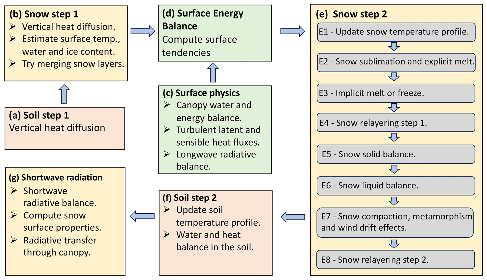
Figure 2 A schematic representation of the main model steps in GLASS and their interface to other relevant physical processes in GFDL LM 4.1.

After performing the energy balance, the following steps are computed. Fresh snow is added to the snowpack in the presence of snowfall (E5). The model first tries to add the new snow to the uppermost existing layer. If the snowfall mass exceeds a threshold, a variable number of layers is added to the top of the snowpack. We then perform the liquid balance in the snowpack (E6): liquid precipitation is added to the top layer. The maximum liquid-water capacity of the layer is computed as a fraction of the layer pore space, given by Eq. (24). If this liquid-water content is exceeded, the excess water flows vertically to the underlying layers. This step is followed by the sequential solution of the liquid-water balance for all snow layers down to the bottom of the snowpack. In panel (e, E7), we perform in sequence snow compaction (described in Appendix B) and wet- and dry-snow metamorphism and evaluate the effect of wind drift (see Appendix A). Finally, at each time step we also re-layer the snowpack in two steps (panel e, E4 and E8), trying to merge or split existing layers based on their distance from the optimal layering structure for the given snow depth, as discussed in Sect. 3.1. After computing this second snow physics step, the new integral properties of the near-surface snow layer are computed. The near-surface layer is defined as the top 3 cm or the entire snowpack, whichever is smaller. These properties are then used to compute snow albedo (panel g) as discussed in Sect. 3.12.

4 Data and methods

4.1 Forcing and validation data

To test model performance, we employ a reference dataset widely used in the snow modeling community (Ménard et al., 2019) and used, for example, in the SnowMIP project (Krinner et al., 2018; Menard et al., 2021). Details for each observation site are reported in Table 2, and the location of the sites is shown in Fig. 3. The 10 sites span a range of climates, elevations, and terrain types. In particular, three of the sites are forested, while the other seven are characterized by either bare soil or grass and low vegetation. The three forested sites located in the Canadian boreal forest are described in Bartlett et al. (2006).

Table 2 Experimental sites used for model validation.

Figure 3 Sites used for model validation. Information about the sites is reported in Table 2.

For this reason, for the seven sites with little to no vegetation we run the model turning off vegetation. For the three forested sites, the long spinup allows model vegetation to fully develop before starting the historical run with in situ meteorological forcing. We force two of the sites (OJB, OBS) to grow evergreen vegetation, while for the third (OAS) we force deciduous species only, to match the existing vegetation types.

In this dataset, each site includes both in situ meteorological forcing for the observation period (as reported in Table 2) and a locally corrected Global Soil Wetness Project Phase 3 (GSWP3) forcing dataset (Ménard et al., 2019) for the period 1980–2015. This forcing dataset is used here to spin the model up for each station up to the year when the in situ meteorological observational record began. After that point, the experiment is run forcing the model with in situ data. Both GSWP3 and in situ forcing data are at hourly temporal resolution and are interpolated at the model 30 min time step. Atmospheric forcing input to LM 4.1 includes liquid and frozen precipitation, downward radiation (direct and diffuse for both visible and near-infrared bands), longwave radiation, air temperature, humidity, pressure, and wind speed. At the Col de Porte site, measurements are done at a constant height above the snow surface. However, this is not the case for the other sites in the dataset, and the model does not correct for the varying height of the measurements above the surface when calculating turbulent fluxes at the snow surface. The dataset forcing only provides total downward shortwave radiation; in our experimental setup, this was divided between direct and diffuse (0.46 and 0.54 of the total flux, respectively) as well as in the visible and near-infrared bands (0.41 and 0.59, respectively) using average climatological values obtained from the GFDL AM4.0 (Zhao et al., 2018) atmospheric model output.

4.2 Experimental setup

In order to perform a meaningful comparison between model and observations, we need to obtain a suitable initial condition for the state of the land model. This is done by performing a model spinup in which key land variables (e.g., vegetation if present, water and heat content in the soil) evolve driven by the atmospheric forcing observed at each site. We found that for all sites presented here in our model, the soil is not frozen during the summer and that the equilibration times characteristic for equilibrium are reached after less than 20 model years of model run. For model spinup, we use at each study site the corrected GSWP3 data provided by Ménard et al. (2019). The model spinup runs for 200 years from 1781 to 1981, cycling through the forcing for the decade 1981–1991. This allows the soil to equilibrate and vegetation to grow at the sites where it is present, i.e., at the three Canadian Boreal Ecosystem Research and Monitoring Sites (BERMS).

After the spinup, the model is run using GSWP3 forcing data up to the date when in situ forcing measurement starts, which for each site is shown in Table 2. Then, the actual experiment is run for the entire length of the in situ forcing dataset. As the model is designed for long climate simulations, it is important that mass and energy are conserved with good accuracy throughout a simulation. Mass and energy conservation are strictly enforced in the model: in the current application, we run the model checking at each model physics time step (30 min) so that conservation violations do not exceed 10⁻⁷ Kg m⁻² for water and 10⁻⁶ J m⁻² for energy.

4.3 Performance metrics

For a description of statistical model performance metrics, we follow Lafaysse et al. (2017). To assess the improvement in model performance due to the new snow scheme, we compute a set of goodness-of-fit measures. For model configuration i (e.g., i is LM-GLASS or i is LM-CM) we compute the bias (${\widehat{B}}_i$) and root-mean-square error (${\widehat{R}}_i$) as

$$\begin{array}{}\text{(37)}& {\widehat{B}}_i={\displaystyle \frac{\mathrm{1}}{N_i}}\sum _{k=\mathrm{1}}^{N_i}(m_{k_i}-o_k)\end{array}$$

and

$$\begin{array}{}\text{(38)}& {\widehat{R}}_i={\left[{\displaystyle \frac{\mathrm{1}}{N_i}}\sum _{k=\mathrm{1}}^{N_i}(m_{k_i}-o_k{)}^{\mathrm{2}}\right]}^{\mathrm{0.5}},\end{array}$$

where N_i model simulated values ($m_{k_i}$) are compared to N_i observed values (o_k).

5 Results

5.1 Bulk snow properties

Simulating the seasonal evolution of the snowpack over the 10 SnowMIP sites allows the demonstration of the behavior of the land model with the new GLASS snow scheme (LM-GLASS) model over a wide range of climate conditions. Time series of snow water equivalent (SWE; defined here in kg m⁻² of snow) is reported in Fig. 4 for all sites. For each site, we show the last 6 snow years of the simulation, including as a benchmark the results from old snow model LM-CM. Overall, both models appear in good agreement with observations for most stations and simulated snow years. Depending on the station, LM-GLASS produces SWE estimates that are either very similar to the old LM-CM snow scheme or larger in magnitude. The latter is the case for the SWA, SNB, and WFJ sites. In these cases, the larger SWE magnitudes predicted by LM-GLASS are closer to observations. These differences in SWE predictions primarily originate from the difference in modeled snow optical properties, with predicted broadband albedo values that tend to be lower for the LM-CM model. For example, for the SWA site, with some of the largest differences between the two models, the BRDF albedo scheme used in LM-CM leads to a significant underestimation of daily albedo (Fig. 5a). This underestimation is not present in the LM-GLASS albedo scheme. For the three BERMS forested sites (OJP, OBS, and OAS) where the model simulates the effects of a multilayer canopy on radiative fluxes, the SWE predictions of the two models are much closer (Fig. 5b). However, in this case modeled and observed albedo values differ significantly in both LM-GLASS and LM-CM. Arguably, this behavior primarily originates from the fact that the vegetation structure produced for the model at this site does not match the dense canopy of the experimental site.

Figure 4 Comparison of predicted SWE between LM-CM (orange) and LM-GLASS (blue). Manual observations (and automatic observations for sites where these are available) are reported by black markers.

Figure 5 Comparison of predicted daily averaged broadband albedo for the Swamp Angel (SWA) site (a) and the BERMS Old Black Spruce (OBS) site (b). Model results are shown for LM-CM (dashed orange lines) and LM-GLASS (solid blue lines). Daily albedo observations are reported by black markers.

When comparing snow depths predicted by the two models, again LM-GLASS yields generally larger snow depths compared to LM-CM (Fig. 6). This behavior is not limited to the sites characterized by appreciable SWE differences between the two models. For instance, in the case of the three BERMS forested sites, LM-GLASS predicts thicker snowpacks despite predicting virtually the same SWE, indicating lower snow density than the constant value used in LM-CM.

Figure 6 Comparison of predicted snow depth between LM-CM (orange) and LM-GLASS (blue). Manual observations (and automatic observations for sites where these are available) are reported by black markers.

5.2 Model performance metrics over the SnowMIP sites

To quantify the relative performance of the two model configurations, we compute the metrics introduced in Sect. 4.3 for all sites, namely bias and RMSE. To attribute the change in model performance to revised snow optical properties or to other snow physical properties, we compare the old snow scheme (LM-CM) to not only the new snow model (LM-GLASS) but also a version of GLASS in which the original BRDF albedo model is retained (LM-GLASS-BRDF). Error metrics for these three model configurations were computed for daily SWE, snow depth, surface albedo soil temperature, and surface snow temperature for all sites where observations of these variables were available.

The LM-GLASS-BRDF model produces little improvement in SWE compared to LM-CM. A general underestimation of the SWE is observed for both models at all sites. On the other hand, this bias is generally reduced in LM-GLASS simulations, leading to a substantial improvement in SWE estimates, as shown in Fig. 7a.

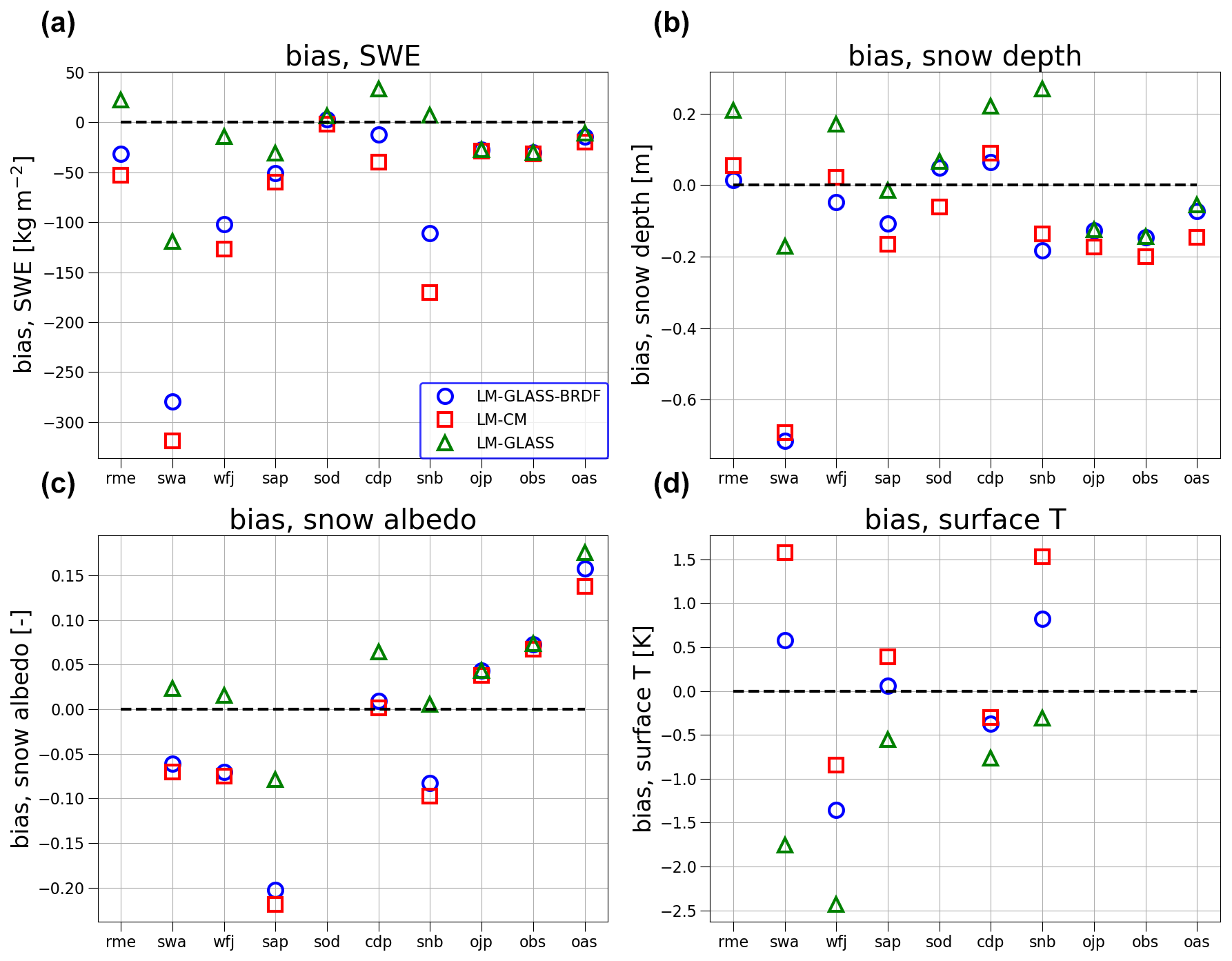
Figure 7 Model bias in SWE (a), snow depth (b), albedo (c), and surface temperature (d) at the 10 SnowMIP sites. Results for each variable are shown for all sites where observations are available.

When considering predictions of snow depth, the difference in performance between the models is less marked compared to SWE results (Fig. 7b). LM-CM generally exhibits a small overestimation, which is mitigated in the case of LM-GLASS-BRDF. In the case of LM-CM, this result implies that the snow density in the model, which is constant, is lower than observations, given the underestimation observed for SWE. When the full LM-GLASS model is considered, multiple sites show modest positive model biases in snow depth. Since SWE predicted by LM-GLASS is the best between the three model configurations, these discrepancies in snow depth also arise from an underestimation in snow density, which in LM-GLASS is primarily driven by the process of snow compaction described in Appendix B.

For daily snow albedo (Fig. 7c), LM-GLASS performs better than both LM-GLASS-BRDF and LM-CM, which generally underestimate daily albedo. An exception to this behavior is observed for two of the BERMS sites, where all models significantly overestimate surface albedo. We argue that this is a consequence of the land model's failure to correctly represent vegetation characteristics and snow–vegetation interactions at these sites, as already shown in the case of albedo at the OBS site reported in Fig. 5b. The effect of the revised albedo model in LM-GLASS is negligible at these forested sites, where a large role is played by the energy balance of canopy layers above the snow. Differences in predicted albedo are very small between LM-CM and LM-GLASS-BRDF. This is not surprising since these two snow schemes have identical BRDF albedo specifications and any differences between the two models thus arise as a consequence of different snow surface temperature values, temperature being the only snowpack property used in the BRDF albedo parameterization.

Finally, biases in snow surface temperature are reported in Fig. 7d for the sites where this variable was recorded. For this variable, the new LM-GLASS model exhibits a larger negative bias compared to LM-CM. Since the bias is also smaller for LM-GLASS-BRDF than for LM-GLASS, this behavior is at least in part connected to the larger surface reflectivity, which however does agree with daily albedo observations, as shown in Fig. 7c. As an example, 3 snow years of daily surface temperature from model simulations and observations for the Col de Porte site are shown in Fig. 8. Here it can be seen that while overall temperature variations are consistent between models and observations, cold-temperature extremes during winter are several degrees lower in the case of LM-GLASS.

Figure 8 Comparison of predicted daily average surface temperature between the LM-CM (dashed orange line) and LM-GLASS (solid blue line) models for the Col de Porte site. Observed values (daily averages) are reported as black markers.

A potential reason for the colder snow surface values predicted by LM-GLASS is that the near-surface snow layers in LM-GLASS can be thinner than those in LM-CM, especially in the case of thick snowpacks. In this case, it is not surprising that thin surface layers with low heat capacity and the increased insulating properties of the underlying snow layers would lead to a colder surface temperature. While this could be a limitation of LM-GLASS, it is also possible that cold temperatures at the surface originate from discrepancies between modeled and actual turbulent fluxes in the atmospheric surface layer. For all the snowpack variables, RMSE was also computed to complement bias and is reported in Fig. 9.

Figure 9 For each model configuration, RMSE metrics for daily SWE (a), snow depth (b), albedo (c), and surface temperature (d) at the 10 SnowMIP sites. Results are reported for all sites where observations are available. Higher RMSE values correspond to poorer model performance.

When examining error metrics in soil temperature, there are important differences between LM-CM and LM-GLASS (Fig. 10). LM-CM exhibits a consistent negative bias of up to −2.5 K at all sites examined here. This bias in soil temperature is greatly mitigated in LM-GLASS. This improvement in soil temperature is also observed in case of LM-GLASS-BRDF, indicating that this behavior is not directly related to the update in snow optical properties. Rather, we argue that the improvement originates in a refined representation of snow heat conductance. LM-GLASS is characterized by not only a finer vertical discretization of the snowpack but also the explicit representation of snow compaction. Snow heat conductance in LM-GLASS is explicitly modeled as a function of snow density. Therefore, the insulating properties of snow with respect to the underlying soil layers are more realistic in LM-GLASS, although a small negative bias remains, indicating that to some extent the actual snow heat conductance could be smaller than that predicted by LM-GLASS. As a representative example of the performance of the models in capturing temperature variations in the underlying soil, we show results for soil temperature at three depths for the Col de Porte site, for which observations are available (Fig. 11). Modeled values are overall consistent with observations, although for the deeper layer, a cold bias is observed for both models. However during the winter season when snow is on the ground, the LM-GLASS-predicted temperatures greatly reduce the cold bias observed for the original model, LM-CM.

Figure 10 Model bias and RMSE for soil temperature. For each site, error metrics were computed for the uppermost soil depth at which observations were available.

Figure 11 Observed and predicted soil temperature for 3 snow years at the Col de Porte site. Observations (black circles) and model-predicted values (LM-CM as dashed orange lines and LM-GLASS as solid blue lines) are reported at three soil depths.

5.3 Implications of the implicit scheme to solve phase change

The treatment of melting and freezing processes can be dependent on the numerical scheme used to resolve these processes. To investigate this issue in LM-GLASS, we examine the differences in the two schemes discussed in Sect. 3.8. SWE predictions obtained from LM-GLASS with the default explicit melt scheme are compared with the same predictions from the implicit scheme. As discussed in Sect. 3.8, in the latter case the change in phase for each snow layer is computed only after the temperature profile is updated from solving the heat transfer through the snowpack implicitly. The differences between explicit and implicit melt schemes are shown in Fig. 12 (panels a and b, respectively). In the case of implicit melt, the modeled SWE exhibits a marked dependence on the time step used in the calculations, with longer time steps leading to an underestimation of the snowmelt. On the other hand, when explicit melt is included in the model as is the case for the default LM-GLASS configuration, this undesirable dependence on the time step effectively disappears. Within the range of time steps examined here (ranging from 5 to 30 min) the results of the explicit melt scheme are closer to the implicit melt results obtained for a 5 min time step. However, while this model time resolution may be attainable for local studies, it is still out of reach for global-scale climate simulations. For a time step of 30 min, which is currently used in global simulations with GFDL LM 4.1, the difference between the two model configurations can become significant.

Figure 12 Time step dependence for the implicit melt (IM) and explicit melt (EM) numerical schemes used for snowmelt. Results are shown for 3 snow years at the Col de Porte site. Manual and automatic SWE observations are reported as black circles and star markers, respectively. Model results obtained by varying the numerical time step used in LM GLASS are reported for each case. Note that in panel (b) the results are virtually independent of the time step, so the three lines overlap.

6 Discussion

A key improvement using LM-GLASS is the increase in winter soil temperature below the snowpack. It has been reported that ESMs participating in the Intergovernmental Panel on Climate Change (IPCC) often underestimate soil temperature, especially at high latitudes (Koven et al., 2013), and this is also the case for the GFDL model. Correcting this bias has important implications for the correct representation of biogeochemical cycles, as warmer soil can lead to climate feedbacks due to the release of greenhouse gases from thawing permafrost. On the other hand, existing cold biases at the snow surface are not resolved in LM-GLASS and are even exacerbated in some cases examined at our experimental test sites. Cold temperatures observed at nighttime are common to other snow models. For example, they have been reported in the CLASS snow model (Brown et al., 2006) and are inevitably heavily dependent upon the atmospheric surface layer scheme used to compute sensible and latent heat fluxes.

According to the classification by Boone and Etchevers (2001), the new LM-GLASS model presented here belongs to the category of high-detail snow schemes. However, the optical properties are characterized by a relatively simple parameterization (based on He et al., 2018b) compared to the fully resolving models such as SNICAR (Flanner and Zender, 2005) or TARTES (Libois et al., 2013). Improvement in snow radiative properties is thus possible. For instance, adding the radiative effect of light absorbing impurities deposited on snow to LM-GLASS will be examined in a companion paper. On the other hand, the snow optical model adopted in GLASS accounts for the effect of snow grain size and shape, which was not done in LM-CM. This development improves predictions of both daily snow albedo and SWE.

Both snow schemes compared here (LM-GLASS and LM-CM) are based on an implicit numerical scheme. This choice is made to ensure numerical stability, given the relatively large time step (∼30 min) used in global climate simulations. However, computations of the phase change within the snowpack is performed according to the explicit melt approach, in which an estimate of the freezing/melting rate is obtained when the surface energy balance is performed. Comparing this approach with a simpler method sometimes used in snow models (i.e., first updating the temperature profile by solving the heat diffusion through the snowpack and only in a second step evaluating freezing or melting rates), we found that in the latter case model predictions are overly dependent on the time step used in the numerical solution. Therefore, this analysis supports the choice of the explicit melt scheme employed in both LM-CM and LM-GLASS. While here the model was applied at point sites so as to mimic observational datasets, GFDL LM 4.1 is routinely employed in global simulations at a relatively coarse resolution (e.g., 1°×1° resolution). In such a case, further research would be necessary to improve the current model with a focus on transitions between snow and no-snow areas, especially over complex terrain. Recent approaches used to model land surface heterogeneity could be useful for this purpose (Chaney et al., 2018; Zorzetto et al., 2023).

Given the increased model complexity of LM-GLASS with respect to LM-CM, it is important to investigate the increased computational cost for the land model. The average increase in runtime for LM-GLASS compared to LM-CM is 7.4 % (with a standard deviation of 7.1 % across the test sites) when considering only the fast 30 min time step of the model in which snow physics is resolved. When considering the change in runtime for the entire land model, we find that the increase in computational cost reduces to 5.6 %. Furthermore, we note that for most of the sites here, the model is run without vegetation, which is a computationally costly component of the land model. We expect therefore that in the presence of vegetation, the relative cost of the LM-GLASS snow model will be lower. For example, when considering only the three BERMS vegetated sites, we found that introducing LM-GLASS increases the cost of the land model only by 3.6 %. Note that these results are only indicative of locations dominated by seasonal snow. However, we note that as snow depth increases, the thickness of the deeper snow layers also increases such that the number of snow layers in LM-GLASS increases relatively slowly with snow depth. We believe additional analysis should be done to assess the performance of GLASS over different settings such as arctic regions and glaciers. Both models compared here tend to have larger biases in the forested sites compared to the other sites, especially for daily surface albedo measured at two of the sites. This is to some extent expected, as vegetation in the model is dynamic and does not necessarily match the real canopy structure at the test sites, which can also be affected by local processes or disturbance history. Interactions of the snowpack and multilayer canopy are a known modeling challenge and should be the focus of future research.

7 Conclusions

We have presented here a new snow model (LM-GLASS) tailored to the GFDL Earth System Model. While maintaining an implicit solution for the energy balance at the snow surface, the new model provides a detailed representation of the snowpack and its interactions with soil, vegetation, and the lower atmosphere. The vertical discretization of the snowpack is now more refined, evolving dynamically based on deposition of fresh snow, sublimation, and snowmelt, and performs within computational constraints. This novel vertical structure allows LM-GLASS to describe vertical variations in snow properties (snow density and grain size and shape), which in LM-GLASS evolve dynamically in each snow layer according to the laws of snow compaction, wind drift, and wet- and dry-snow metamorphic processes.

Analysis of the performance of LM-GLASS and comparison with a simpler snow model (LM-CM) previously used in the GFDL land model showed the relevance of accounting for these additional physical processes. By evaluating the model performance over 10 SnowMIP sites, we found an overall improvement in how the model represents SWE and comparable results for snow depth between the two models. The observed improvement in SWE predictions primarily originates from the updated snow optical properties, which in LM-GLASS explicitly depend on snow optical diameter and grain shape. We found that the BRDF parameterization used in LM-CM tends to underestimate albedo at the test sites in general (by about 0.05 for sites with no vegetation) and thus can lead to overestimating snowmelt.

The largest improvement(and the one more consistent across sites) in model skill was found for soil temperature, which was generally underestimated by about 1.5° C in LM-CM, suggesting an overestimation in heat conductance through the snowpack. In LM-GLASS, soil temperature predictions were on average higher than those obtained from LM-CM during the snow accumulation phase at all sites and were generally closer to observations at sites where these were collected. The increased model complexity of LM-GLASS is due to a combination of refined vertical resolution and additional physical processes resolved in the model. These features lead to a computational cost increase of about 5.6 % for the resulting land model (LM-GLASS) on average over the test sites. The development of a refined snow model and its implementation in an Earth system model paves the way towards multiple future improvements and research directions. First, future work could investigate the performance of the snow scheme globally and in coupled land–atmosphere simulations, necessary to evaluate the strength of any feedbacks originating from the improved realism in snow physics. LM-GLASS is expected to impact land–atmosphere interactions due to the changes in (i) snow albedo, (ii) snow surface temperature, and (iii) soil temperature. The last feature is particularly encouraging, as several ESMs (including the GFDL model) have been found to broadly underestimate soil temperature with important implications, e.g., for permafrost simulation. Finally, future research could further improve the description of snow optical properties harnessing the vertical information on snow grain properties provided by LM-GLASS. Towards this objective, in a companion paper we will present the effects of deposition of light absorbing impurities in LM-GLASS and their effect on snow albedo and snowmelt.

Appendix A: Effect of wind on snow

The effect of wind on snow implemented in GLASS is based on the approach used in CROCUS (Brun et al., 1997; Vionnet et al., 2012), with the only difference being that GLASS tracks three snow variables as prognostic (snow dendricity, sphericity, and optical diameter), consistent with the approach used for snow metamorphism. A mobility index parameter M_0,k quantifies the vulnerability of a snow layer to wind erosion,

$$\begin{array}{}\text{(A1)}& M_{\mathrm{0},k}=\left\{\begin{array}{ll}\mathrm{0.34}(\mathrm{0.75}{\mathit{\delta }}_k-\mathrm{0.5}{s}_{\mathrm{p},k}+\mathrm{0.5})+\mathrm{0.66}{F}_{{\mathit{\rho }}_k}& \\ & \mathrm{\text{for dendritic snow}}\\ \mathrm{0.34}(-\mathrm{0.583}{g}_{\mathrm{s},k}-\mathrm{0.833}{s}_{\mathrm{p},k}+\mathrm{0.833})& \\ +\mathrm{0.66}{F}_{{\mathit{\rho }}_k}& \mathrm{\text{for non-dendritic snow,}}\end{array}\right.\end{array}$$

with $F_{{\mathit{\rho }}_k}=\mathrm{1.25}-\mathrm{0.0042}(max({\mathit{\rho }}_{min},{\mathit{\rho }}_k)-{\mathit{\rho }}_{min})$, with ${\mathit{\rho }}_{min}=\mathrm{50}$ kg m⁻³, and with $g_{\mathrm{s},k}={\mathit{\alpha }}_M(\mathrm{4}-s_{\mathrm{p},k})$, ${\mathit{\alpha }}_M={\mathrm{10}}^{-\mathrm{4}}$. A driftability index is then obtained as $S_{\mathrm{l},k}=-\mathrm{2.868}\exp (-\mathrm{0.085}\stackrel{\mathrm{‾}}{U})+\mathrm{1}+M_{\mathrm{0},k}$, accounting for the effect of the average wind speed $\stackrel{\mathrm{‾}}{U}$, so wind-driven snow transport occurs only for $S_{\mathrm{l},k}>\mathrm{0}$. The effect of wind drift on snow microstructure is accounted for by evolving snow grain properties as a consequence of packing and fragmentation by the wind action. The characteristic timescale of this process for a snow layer is computed as ${\mathit{\tau }}_{\text{WD},k}=\frac{{\mathit{\tau }}_{\text{w0}}}{{\mathrm{\Gamma }}_{\text{WD},k}}$, with ${\mathrm{\Gamma }}_{\text{WD},k}=max(\mathrm{0},S_{\mathrm{l},k}\exp (-{\mathit{\zeta }}_{\text{WD},k}/\mathrm{0.1}\left)\right)$ and τ_w0=48 h. Here ζ_WD,k is a depth scale in the snowpack that accounts for the hardening of overlying layers and reads ${\mathit{\zeta }}_{\text{WD},k}={\sum }_{i<k}\left(\mathrm{\Delta }{z}_i\right(\mathrm{3.25}-S_{\mathrm{l},i}\left)\right)$. The evolution of snow properties due to snow drift is computed as in CROCUS. LM-GLASS evolves sphericity, dendricity, and optical diameter of snow. Additionally, snow density also evolves according to the equation

$$\begin{array}{}\text{(A2)}& {\displaystyle \frac{\mathrm{d}{\mathit{\rho }}_k}{\mathrm{d}t}}={\displaystyle \frac{{\mathit{\rho }}_{\text{max}}-{\mathit{\rho }}_k}{{\mathit{\tau }}_{\text{WD},k}}},\end{array}$$

with ρ_max=350 kg m⁻³. For dendritic snow we have

$$\begin{array}{}\text{(A3)}& {\displaystyle \frac{\mathrm{d}{s}_{\mathrm{p},k}}{\mathrm{d}t}}={\displaystyle \frac{\mathrm{1}-s_{\mathrm{p},k}}{{\mathit{\tau }}_{\text{WD},k}}}\text{(A4)}& {\displaystyle \frac{\mathrm{d}{\mathit{\delta }}_k}{\mathrm{d}t}}={\displaystyle \frac{{\mathit{\delta }}_k}{\mathrm{2}{\mathit{\tau }}_{\text{WD},k}}}\text{(A5)}& {\displaystyle \frac{\mathrm{d}{d}_{\text{opt},k}}{\mathrm{d}t}}={\mathit{\alpha }}_M\left[{\displaystyle \frac{{\mathit{\delta }}_k}{\mathrm{2}{\mathit{\tau }}_{\text{WD},k}}}(s_{\mathrm{p},k}-\mathrm{3})+({\mathit{\delta }}_k-\mathrm{1}){\displaystyle \frac{\mathrm{1}-s_{\mathrm{p},k}}{{\mathit{\tau }}_{\text{WD},k}}}\right],\end{array}$$

while for non-dendritic snow

$$\begin{array}{}\text{(A6)}& {\displaystyle \frac{\mathrm{d}{d}_{\text{opt},k}}{\mathrm{d}t}}=-\mathrm{2}{\mathit{\alpha }}_M{s}_{\mathrm{p},k}{\displaystyle \frac{\mathrm{1}-s_{\mathrm{p},k}}{{\mathit{\tau }}_{\text{WD},k}}}\text{(A7)}& {\displaystyle \frac{\mathrm{d}{s}_{\mathrm{p},k}}{\mathrm{d}t}}={\displaystyle \frac{\mathrm{1}-s_{\mathrm{p},k}}{{\mathit{\tau }}_{\text{WD},k}}}.\end{array}$$

Redistribution of snow across model grid cell or tiles is not implemented at this stage; however, we note that this issue is generally more relevant for local studies on small horizontal scales rather than the grid cell scale of the climate-focused LM 4.1.

Appendix B: Effect of snow compaction

Snow compaction is described following the approach used in the CROCUS model (Vionnet et al., 2012). The mechanical settling of each snow layer $k=\mathrm{1},\mathrm{\dots }{n}_{\mathrm{L}}$ is computed as

$$\begin{array}{}\text{(B1)}& {\displaystyle \frac{\mathrm{d}\mathrm{\Delta }{z}_k}{\mathrm{\Delta }{z}_k}}=-{\displaystyle \frac{{\mathit{\sigma }}_k}{{\mathit{\eta }}_k}}\mathrm{d}t,\end{array}$$

with σ_k the vertical stress due to the weight of overlying snow layers (${\mathit{\sigma }}_j=\frac{\mathrm{1}}{\mathrm{2}}g{\mathit{\rho }}_k\mathrm{\Delta }{z}_k+{\sum }_{j=\mathrm{1}}^{k-\mathrm{1}}g{\mathit{\rho }}_j\mathrm{\Delta }{z}_j$, neglecting the effect of local slope, and with g=9.806 m s⁻²). The snow layer viscosity η_k is parameterized as

$$\begin{array}{}\text{(B2)}& {\mathit{\eta }}_k=f_{\mathrm{1}}{f}_{\mathrm{2}}{\mathit{\eta }}_{\mathrm{0}}{\displaystyle \frac{{\mathit{\rho }}_k}{c_{\mathit{\eta }}}}{e}^{a_{\mathit{\eta }}(T_{\mathrm{F}}-T_k)+b_{\mathit{\eta }}{\mathit{\rho }}_k},\end{array}$$

with ${\mathit{\eta }}_{\mathrm{0}}=\mathrm{7.62237}\times {\mathrm{10}}^{\mathrm{6}}$ $\mathrm{kg}{\mathrm{s}}^{-\mathrm{1}}{\mathrm{m}}^{-\mathrm{1}}$, a_η=0.1 K⁻¹, b_η=0.023 m³ kg⁻¹, and c_η=250 kg m⁻³. The factors $f_{\mathrm{1}}=\mathrm{1}/(\mathrm{1}+\mathrm{60}{\mathit{\theta }}_{\mathrm{L},k})$ and $f_{\mathrm{2}}=min(\mathrm{4},\exp (min(g_{\mathrm{1}},\mathrm{0.5}{g}_{\mathrm{s}}-g_{\mathrm{2}})/g_{\mathrm{3}}\left)\right)$ account for the presence of liquid water and the grain size effects on viscosity, respectively. Here g₁=0.4 mm, g₂=0.2 mm, and g₃=0.1 mm; $g_{\mathrm{s},k}={\mathit{\alpha }}_M(\mathrm{4}-s_{\mathrm{p},k})$ as in (Carmagnola et al., 2014); and ${\mathit{\theta }}_{\mathrm{L},k}=w_{\mathrm{l},k}/\left({\mathit{\rho }}_{w,k}\mathrm{\Delta }{z}_k\right)$ is the liquid-water content of the snow layer.

Appendix C: LM-CM BRDF snow albedo model

For the purposes of computing the surface albedo in the case of little snow on the ground, fractional snow cover is computed based on snow depth as follows:

$$\begin{array}{}\text{(C1)}& f_{\text{snow}}={\displaystyle \frac{h_{\mathrm{s}}}{h_{\mathrm{s}}+h_{\mathrm{s},\mathrm{c}}}},\end{array}$$

where h_s is the total snowpack depth and $h_{\mathrm{s},\mathrm{c}}=\mathrm{0.0167}$ m in a typical model configuration. Equation (C1) is used in all model configurations compared in this paper. We remark that, as noted in Dutra et al. (2010), this formulation for the effective snow fractional area to some extent accounts for the effect of snow density, as it is based on snow depth rather than on SWE, so the same mass of snow generally corresponds to a smaller fractional area in the spring snow melting phase. The snow albedo model used in the current version of the model (GFDL LM 4.1 CM) is based on an empirical bidirectional reflectance distribution function (BRDF) by Schaaf et al. (2002). According to this model, black-sky albedo is expressed as

$$\begin{array}{}\text{(C2)}& {\displaystyle }\begin{array}{rl}{\displaystyle }{\mathit{\alpha }}_{\text{bs}}\left(\mathit{\theta }\right)=& {\displaystyle }{f}_{\text{iso}}(g_{\mathrm{0},\text{iso}}+g_{\mathrm{1},\text{iso}}{\mathit{\theta }}^{\mathrm{2}}+g_{\mathrm{2},\text{iso}}{\mathit{\theta }}^{\mathrm{3}})\\ {\displaystyle }& {\displaystyle }+f_{\text{vol}}(g_{\mathrm{0},\text{vol}}+g_{\mathrm{1},\text{vol}}{\mathit{\theta }}^{\mathrm{2}}+g_{\mathrm{2},\text{vol}}{\mathit{\theta }}^{\mathrm{3}})\\ {\displaystyle }& {\displaystyle }+f_{\text{geo}}(g_{\mathrm{0},\text{geo}}+g_{\mathrm{1},\text{geo}}{\mathit{\theta }}^{\mathrm{2}}+g_{\mathrm{2},\text{geo}}{\mathit{\theta }}^{\mathrm{3}}),\end{array}\end{array}$$

with θ the solar zenith angle. The white-sky albedo reads

$$\begin{array}{}\text{(C3)}& {\mathit{\alpha }}_{\text{ws}}=f_{\text{iso}}{g}_{\text{iso}}+f_{\text{vol}}{g}_{\text{vol}}+f_{\text{geo}}{g}_{\text{geo}}.\end{array}$$

Given the ratio r_dif of direct-to-total shortwave radiation received by the surface, the blue-sky albedo is then obtained as $\mathit{\alpha }\left(\mathit{\theta }\right)=(\mathrm{1}-r_{\text{dif}}){\mathit{\alpha }}_{\text{bs}}\left(\mathit{\theta }\right)+r_{\text{dif}}{\mathit{\alpha }}_{\text{ws}}$. Here the parameters g_i are universal, given in Schaaf et al. (2002) and reported in Table C1, while f_i depend on the specific surface properties. For snow, two set of parameters are used, corresponding to “cold snow”, characterized by surface temperature below 10 °C, and “warm snow” above freezing (0 °C). Within this temperature range, the snow albedo is obtained by linear interpolation between temperatures estimated for cold and warm conditions. This formulation was introduced to mimic the effect of snow aging at different temperatures in the absence of information about snow microphysical properties.

Table C1 Parameters of the BRDF model with j equal to iso, vol, or geo, and b is the model shortwave band.