CHONK 1.0: landscape evolution framework: cellular automata meets graph theory

Landscape evolution models (LEMs) are prime tools for simulating the evolution of source-to-sink systems through ranges of spatial and temporal scales. A plethora of various empirical laws have been successfully applied to describe the different parts of these systems: fluvial erosion, sediment transport and deposition, hillslope diffusion, or hydrology. Numerical frameworks exist to facilitate the combination of different subsets of laws, mostly by superposing grids of fluxes calculated independently. However, the exercise becomes increasingly challenging when the different laws are inter-connected: for example when a lake breaks the upstream–downstream continuum in the amount of sediment and water it receives and transmits; or when erosional efficiency depends on the lithological composition of the sediment flux. In this contribution, we present a method mixing the advantages of cellular automata and graph theory to address such cases. We demonstrate how the former ensure interoperability of the different fluxes (e.g. water, fluvial sediments, hillslope sediments) independently of the process law implemented in the model, while the latter offers a wide range of tools to process numerical landscapes, including landscapes with closed basins. We provide three scenarios largely benefiting from our method: (i) one where lake systems are primary controls on landscape evolution, (ii) one where sediment provenance is closely monitored through the stratigraphy and (iii) one where heterogeneous provenance influences fluvial incision dynamically. We finally outline the way forward to make this method more generic and flexible.

1 Introduction

The timescale of sediment transport along the source-to-sink system from upstream erosion to downstream deposition is relatively short compared to the timescales of other geological processes. However, its large spatial extent on areas and the sometimes great intermittence of activity make it difficult to measure and observe directly (e.g. Sadler, 1981; Jerolmack and Sadler, 2007; Ganti et al., 2011; Schumer et al., 2017). Various models, analogue and numerical, help explore source-to-sink systems at different temporal and spatial scales that complement field observations. Analogue models offer a time compression in scaled experiments to rapidly simulate long time spans with complex physics but relatively simple environmental forcing (Babault et al., 2005; Paola et al., 2009; Guerit et al., 2014). Alternatively, numerical landscape evolution models (LEMs) have the advantage of giving complete control of the simulation. However, they rely mostly on empirical laws and are often limited to specific geoscience problems. For example, the evolution of surface topography over millions of years can be efficiently explored with erosion laws that only indirectly consider sediment transport in their numerical scheme (e.g. Yuan et al., 2019; Hergarten, 2020) or even completely ignore them (e.g. Braun and Willett, 2013) to the benefit of numerical performance. On the contrary, bedrock incision can be advantageously ignored when the focus is a high-resolution modelling of sediment redistribution at very short time-scales (e.g. Sklar and Dietrich, 1998; Croissant et al., 2017; Coulthard et al., 2013; Roelvink and Van Banning, 1995). A major challenge therefore lies in finding the right combination of laws to best address a given problem (Barnhart et al., 2019). That is complicated by the significant impacts of any change in numerical or physical parameters both in terms of quantitative results and computation time (e.g. Campforts et al., 2017; Armitage, 2019; Grieve et al., 2016).

While some process laws are implemented in stand-alone models (e.g. Hergarten, 2020; Braun and Sambridge, 1997; Coulthard et al., 2013), mature frameworks exist to facilitate the combination of different LEM components and to explore their results (e.g. Barnhart et al., 2020; Bovy, 2019; Schwanghart and Scherler, 2014; Mudd et al., 2019). However, these frameworks and models are designed to combine process laws at grid level where, for example local minima, flow routing or river incision are successively and serially solved. This can be a problem when studying more complex source-to-sink systems with multiple processes that are inter-connected. Let us picture a situation where a lake acts as a local sink. Its sediment and water budget depends on all processes involving sediments or water upstream (Fig. 1). Its filling will, in turn, impact the behaviour of the process law downstream by modifying the amount of water and sediments they will transmit. This is incompatible with grids solved independently, or it requires exchange data structures that increase the run-time exponentially. Beside the question of local minima as in the lake example, the role of sediment fluxes is perhaps the most representative example of inter-connectivity. Sediment starving or an abundance of clasts in a river will impede bedrock erosion by a lack of tools or an excess cover (Sklar and Dietrich, 2004; Finnegan et al., 2007; Geurts et al., 2018). The relative strengths of erosive clasts and erodible bedrock can also significantly enhance or diminish the erosion efficiency of a river and trigger local and non-local consequences (e.g. Gailleton et al., 2021; Sklar and Dietrich, 2001, respectively). Alluvial dynamics matter for source-to-sink studies: aggradation–incision cycles in mountain piedmonts can delay sediment delivery to the ocean by >10 kyr, a climatically relevant timescale, and recycle old signals in the sediment stream (e.g. Clift and Giosan, 2014; Malatesta et al., 2018; Dingle et al., 2020). Modulation of sediment fluxes also leads to prominent alluvial terraces and surfaces that are key for landscape interpretation (Bufe et al., 2017; Tofelde et al., 2017; Malatesta and Avouac, 2018). Increasingly fine resolution in stratigraphic studies warrants a renewed attention to the trajectory of sediment tracers across the landscape (Tofelde et al., 2021). Novel radiometric methods enable the exploitation of new sedimentary signatures that require a precise understanding of the rate and path of transport of sediment across landscapes (e.g. Lupker et al., 2017). Modelling sediment fluxes at the level of details that field and analytical studies can now attain benefits from the holistic approach presented here rather than the independent implementation of individual processes.

In this contribution, we propose a novel methodology, CHONK, to develop frameworks that include fine-grained modularity in a cell-based referential, so as to ensure inter-connectivity between LEM properties. CHONK is built to guarantee unconditional access to a common numerical toolkit regardless of the type of geomorphological laws employed. The cell-based referential allows one to track the parameters and/or to explore the dynamic feedback within the different fluxes transported from one cell to another. We demonstrate the potential of integrating cellular automata elements with graph-based finite difference methods to resolve sedimentary dynamics necessary for sedimentological studies of landscape evolution. This contribution presents the core architecture of CHONK, while several collaborative projects employ and apply the framework to address sedimentological and geomorphological challenges. These projects concurrently inform the development of a user-friendly platform to be progressively released in the coming months and years.

First, we concisely present and explain the new method. We then detail the model structure, its different algorithms, and the process laws we picked for the demonstration. Finally, we present and discuss different scenarios demonstrating the capabilities of this new method.

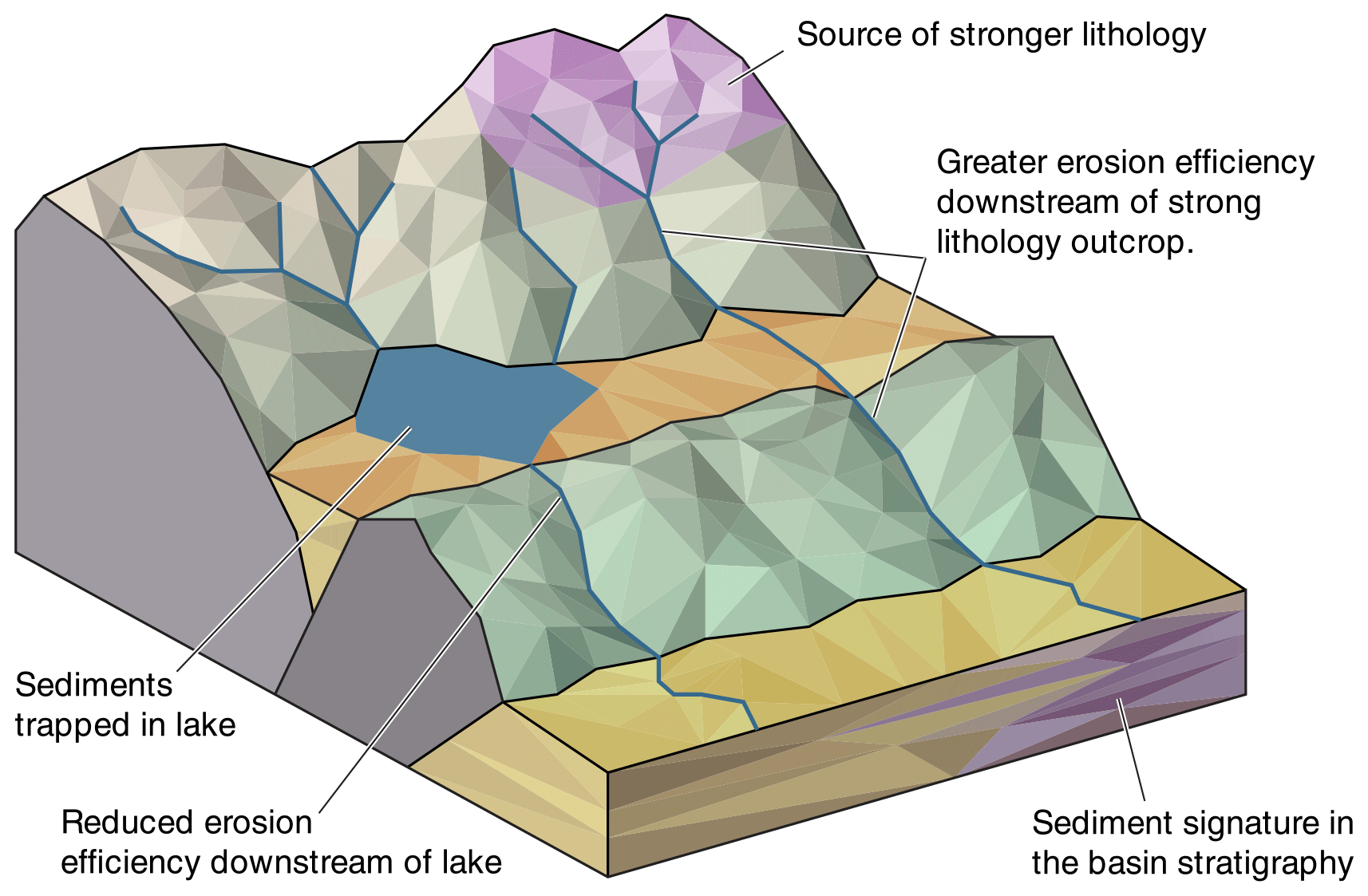
Figure 1 Cartoon landscape highlighting several key attributes of the sedimentary system that CHONK is designed to solve with a novel approach blending cellular automata and graph-based methods. The different domains connected by the river network and hillslope transfers of material highlight the interconnected nature of the different processes.

2 Background and rationale

The new formulation we introduce in this contribution combines the advantages offered by the cellular automata methods (von Neumann, 1951; Wolfram, 1984) and graph-based finite difference methods commonly used in LEMs and frameworks (e.g. Bovy, 2019; Barnhart et al., 2020; Garcia-Castellanos and Jiménez-Munt, 2015; Braun and Willett, 2013). We first briefly define and review the existing methods and framework to explain our rationale for creating a new one.

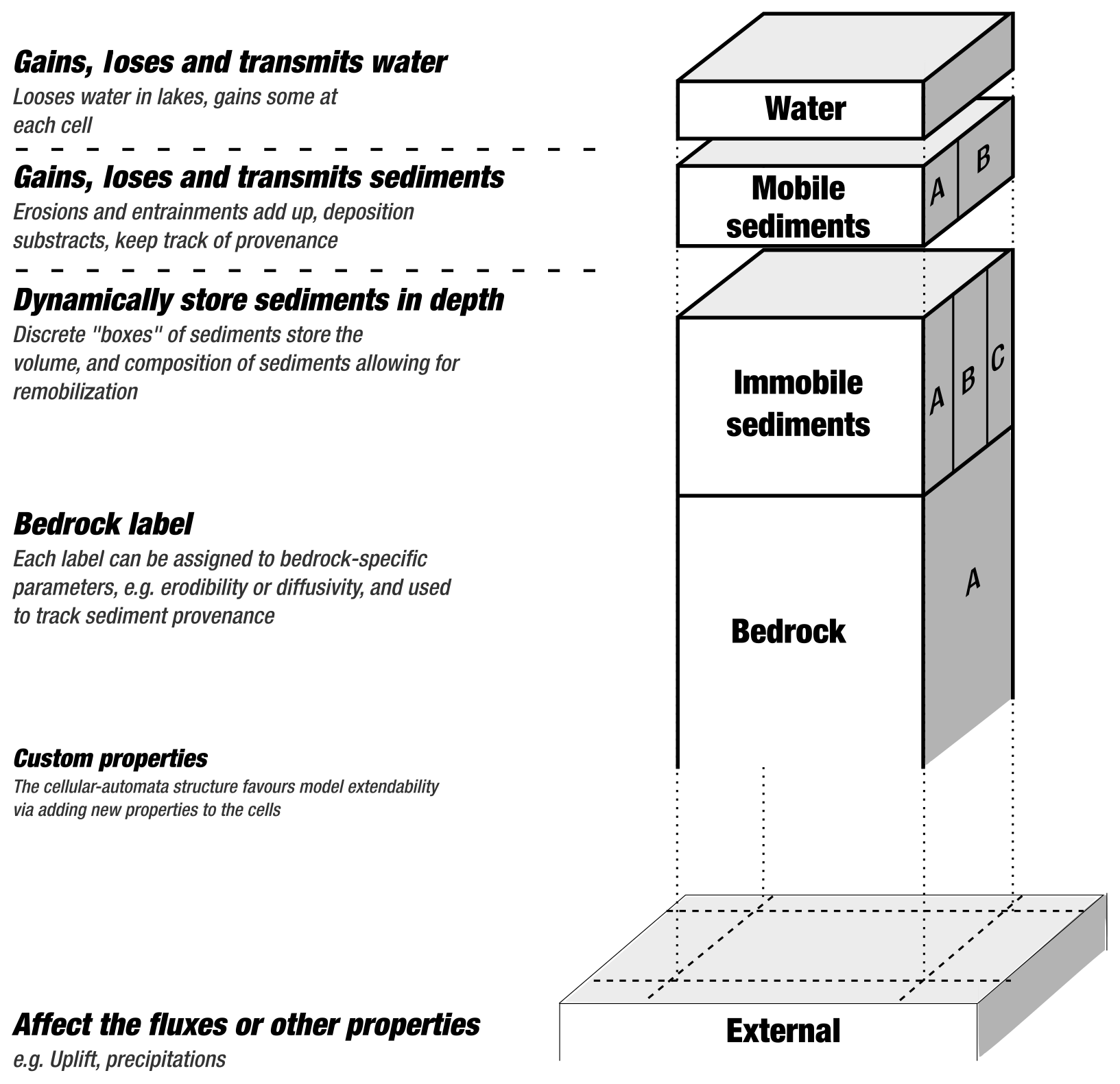
Figure 2 Cartoon illustrating the cellular automata data structure put in place in this model, with an explanation of the cell structure. These cells are then plugged onto a graph, taking advantage of classic LEM algorithms to process the cell in the correct topological order.

2.1 Graph-based frameworks and methods

LEM frameworks typically solve the different components of landscape evolution modelling independently following a graph-based logic applied on data grids. In other words, fluxes and other quantities (e.g. elevation, erosion, water) are discretized on 2D arrays that are calculated and combined successively. Geomorphological processes typically require downstream transfers of fluxes (e.g. drainage area, water or sediments); upstream propagation of numerical schemes (e.g. Braun and Willett, 2013; Campforts et al., 2017); or even successive iterations of both (e.g. Yuan et al., 2019; Hergarten, 2020). LEMs compute those by building a directed acyclic graph (DAG) where each discretized location defines a node (or vertex) with directed link (or edge) towards its downstream neighbour(s). This data structure enables operations such as graph traversals or topological sorting which ensure the required downstream or upstream processing of nodes. LEMs can integrate the graph structure explicitly (i.e. computing the vertex and edge structures), taking advantage of graph theory algorithms such as topological sorting (e.g. Braun and Willett, 2013; Anand et al., 2020) or more sophisticated local-minima processing methods (e.g. Cordonnier et al., 2019; Barnes et al., 2020); they can also use intermediate data structures such as priority queues to navigate in complex, depression-bearing landscapes without having to store edges (e.g. Barnes et al., 2014b); or simply sort nodes by decreasing elevation after eventually processing local minima (e.g. Braun and Sambridge, 1997; Carretier et al., 2016; Hergarten, 2020).

A typical graph-base LEM flow can be illustrated with the stream-power incision model (Howard and Kerby, 1983), a widely used fluvial incision equation where erosion rate is defined as a function of slope and drainage area. LEMs first compute a graph structure to calculate drainage area and weigh it by water influx to have a proxy for water discharge. At this stage, local minima (i.e. lakes, endorheic basins or noise) are filled with water or carved out at this stage in order to ensure flow continuity (e.g. Braun and Willett, 2013; Cordonnier et al., 2019; Barnes et al., 2014b; Salles, 2019). Then the models compute topographic slopes from the previously filled surfaces and finally combine both data grids with an erodibility parameter to calculate fluvial incision rates in each cell. Such grid-based formulation is very flexible and allows for modifications in order to adapt the model to a geoscientific problem. For example adding hillslope diffusion to the workflow (e.g. Roering et al., 1999) would consist in calculating it after fluvial incision and combining the grids of elevation changes at the end of the process. Implementing alternative methods is also straightforward: for example switching from the stream power incision model to a transport-limited one (e.g. Sklar and Dietrich, 1998) only requires replacing the section of the sequential process that deals with the fluvial process.

However, the combination of independently calculated grids reaches its limitations when processes are interdependent (e.g. calculating fluvial incision function of the nature of its upstream sediment input combining all the processes and what could have been stored in potential lakes). Let us consider an example where lakes are of great importance for landscape evolution. They act as intermediate traps in the domain and the amount of sediments and water they may transmit downstream as a function of the overall amount they receive. The influx can only be known if all the processes happening upstream of the lake have been processed. This is not compatible with a sequential treatment of processes and requires specific implementations (e.g. Garcia-Castellanos and Jiménez-Munt, 2015; Salles, 2019) where any modification in the methods or processes requires significant work to redesign its whole implementation. This is not always straightforward, is often highly dependent on the actual numerical format of the LEM and is accompanied by an unavoidable loss of flexibility and modularity.

2.2 Cellular automata method

Cellular automata models are reduced-complexity models designed to tackle discretized problems on networks of connected cells (von Neumann, 1951; Wolfram, 1984). The cells have given properties and states which evolve as a function of the states of their neighbours according to a set of rules. Road traffic modelling by Nagel and Schreckenberg (1992) is a good illustration of cellular automata logic. Cells represent a stretch of road and their properties include, for example the presence or absence of cars, their velocity, or whether they are Honda Jazz. Cells evolve as a function of the presence of cars in their linked counterparts following simple rules to simulate road traffic. Cellular automata methods can also include more sophisticated equations and processes and have been utilized for modelling elements of landscape evolution such as water and sediment fluxes (Coulthard et al., 2013); tracking particles in flow (e.g. Tucker et al., 2016); hillslope evolution (e.g. Tucker and Bradley, 2010; Jyotsna and Haff, 1997); soil erosion (e.g. D'Ambrosio et al., 2001); sediment transport and channel morphology (e.g. Salles et al., 2007). Frameworks exist to take advantage of cellular automata (e.g. Barnhart et al., 2020, partially implemented in Tucker et al., 2016). It is important to note the cells are processed in no particular order and cannot propagate non-local fluxes such as drainage area within a single time step.

2.3 Hybrid solution: cellular automata on a graph

We developed a new formulation combining the advantages of the graph-based and cellular automata methods. The aim is to make generic interactivity between fluxes and processes an intrinsic feature of LEM design. Building on the lake example we used in Sect. 2.1, if a simulation requires the sediment and water budget of a lake, one should be able to edit the processes affecting water and sediment fluxes without having to modify the entire workflow. This requires a number of numerical constraints: (i) fluxes should be defined separately from processes in order to let a theoretically unconditional number of processes affect the fluxes; (ii) the processing of the graph should be as independent as possible of the processes – meaning that the resolving of local minima should not imply they are systematically filled; and (iii) every inter-connected processes should be processed simultaneously within a single location before transmitting fluxes to the next. In this contribution, we present CHONK 1.0, a proof-of-concept for this modelling design with its functional workflow.

To do so, we process a topographic grid from which we calculate a depression-aware graph of downstream/upstream connectivity. The latter does not assume the depression systems will be systematically filled, but instead preprocesses a data structure allowing for different scenarios (i.e. different levels of details in the processing). Every node (i.e. every discretized location as described in Sect. 2.1) on the grid is then treated as a cell only processed in the downstream direction. The properties of the cells are the quantities and fluxes needed by the equations implemented in the model – e.g. elevation, bedrock incision, water, sediment fluxes (Fig. 2). Like cellular automata methods, all the processes affecting fluxes and quantities are processed before transfer to downstream cells. The combination of both methods ensures that when a cell belongs to a topographic depression, the definitive fluxes are known and this information can be used to fill that depression. The cells are processed in a specific order following a topology dictated by the topographic graph. Lakes are just one example benefiting from this method, and we will demonstrate that this method is particularly adapted to solving problems and challenges involving interdependent feedbacks that are difficult to tackle otherwise.

The prototype we developed for this contribution is a first step towards a fully fledged, generic and dedicated framework like Barnhart et al. (2020) or Bovy (2019). We implemented a specific set of process laws in order to test and demonstrate the advantages of this method.

2.4 Comparison with existing models or frameworks

A number of numerical tools already exists for landscape evolution modelling. It is not in the scope of this paper to provide an exhaustive review of all of them, but it is important to mention those most relevant to our goals.

Cellular automata models have been utilized for LEMs at basin scale. Coulthard et al. (2013) developed CAESAR-LISFLOOD, a cellular automaton model approximating the shallow-water equations (Bates et al., 2010) and designed to explore fluvial sediment transport and bedrock erosion over the timescale of few thousand years. Like other LEMs solving similar equations (e.g. Davy et al., 2017; Adams et al., 2017), this family of methods is not designed for geological and/or mountain-range scale because they are (i) numerically limited by the short time steps required to keep the finite difference scheme stable and (ii) philosophically limited by the amount of external constraints required (high-resolution precipitation patterns, for example). CAESAR-LISFLOOD also processes all the cells in any arbitrary order (or even in parallel) and only transfer sediments and water from a cell to its immediate neighbour within a single numerical time step – as opposed to a full landscape traversal per time steps for longer-term LEMs.

The landscape evolution modelling community benefits from well-established frameworks to develop and design LEMs and topographic analysis tools (Barnhart et al., 2020; Schwanghart and Kuhn, 2010; Mudd et al., 2019; Bovy, 2019). They all rely on routines manipulating a topographic grid and building a graph of node connectivity for it. However, existing frameworks are primarily designed to be solved on grids alone and they inherit their limitations (Sect. 2.1).

Accounting for lakes is one of the main features of our method and we note that different approaches already exist. A common family of methods consists in pre-processing local minima by directly altering the topography in order to force an outflow by either carving a way to an output (Lindsay, 2016) or filling them (Wang and Liu, 2006; Barnes et al., 2014a). Both force the local minima to connect to the rest of the landscapes and the flow to escape via the edges. Bovy (2019) utilizes an alternative method by Cordonnier et al. (2019) leveraging graph theory to simulate carving/filling without affecting topography. It is worth noting that some algorithms have been specifically develop to process, calculate and fill depressions with an arbitrarily given amount of water. Among these, the closest to our aim are the developments by Callaghan and Wickert (2019); Barnes et al. (2020, 2021). They designed a set of methods to (i) identify, (ii) hierarchize and (iii) fill the depression with a particular focus on numerical efficiency. It is worth noting that the model developed by Callaghan and Wickert (2019) is a cellular automaton. While we partially built our numerical method to manage lakes on these previous developments, there are a couple of differences, most of them related to our need to integrate the lake solver into a pre-existing multiple-flow graph for node connectivity. More detailed differences are outlined in Sect. 3.3.2. Geurts et al. (2018), for example utilized the method of Braun and Sambridge (1997) to simulate lake filling by stopping flow at the lake bottom and only connecting the lake to the rest of the landscapes once filled with fluvial sediments. Campforts et al. (2020) or Yuan et al. (2019) enhanced fluvial deposition in lake areas in order to roughly approximate lake deposition. These methods acknowledge the importance of lakes in the landscapes, but do not treat them as separate domains with dedicated processes. Salles (2019) characterize lakes by first filling the topography with the approach of Barnes et al. (2014a) and identifying areas of topographic change. Their model then traps all the sediment carried in these domains, transmitting potential excess to the downstream landscape. This method is close to what we aim to achieve but considers lake as unconditionally filled and outletting, thus not designed for endorheic basins. TISC (initially described by Garcia-Castellanos and Jiménez-Munt, 2015) is a pioneer in terms of integrating endorheism to LEMs and recognizing its impact on landscape evolution (Garcia-Castellanos et al., 2003; Garcia-Castellanos, 2006; Struth et al., 2021). TISC calculates the topography of the depressions and fills them gradually with the available sediment and water. Excess material is only transmitted to the outlet and downstream landscapes if available, successfully simulating closed lakes and endorheism when lake evaporation or infiltration balances precipitation. The implementation of TISC, however, is not compatible with our design as water fluxes are calculated separately from the rest of the processes. Runoff is first calculated and the lakes are gradually filled, dynamically accounting for evaporation and lake spilling. Other processes are only calculated after the water flux is defined whereas CHONK calculates all the fluxes simultaneously for each separate cell, allowing inter-connectivity between their properties.

Finally, tracking sediment provenance in LEMs has been done in different ways. Carretier et al. (2016) add discrete Lagrangian particles on top of Eulerian grids. They post-process erosion, entrainment and deposition of sediment fluxes to determine the movement of these particles with a probabilistic approach. Sharman et al. (2019) integrate the erosion field to back-calculate provenance from labelled areas. These existing methods have in common that they are post-processing the tracking, i.e. calculating the proportion of sediment provenance after the calculation of the surface process laws. We aim in this contribution to embed the trackers into the model in order to make possible their integration directly in the process laws, for example adjusting fluvial erosivity to the proportion of a certain rock type in the sediments relative to the local bedrock type.

3 Model implementation

3.1 Generic numerical structure

Before describing the technical details inherent to CHONK 1.0, we provide a generic description of the modelling design – outlining the steps required for a general implementation following the same principles.

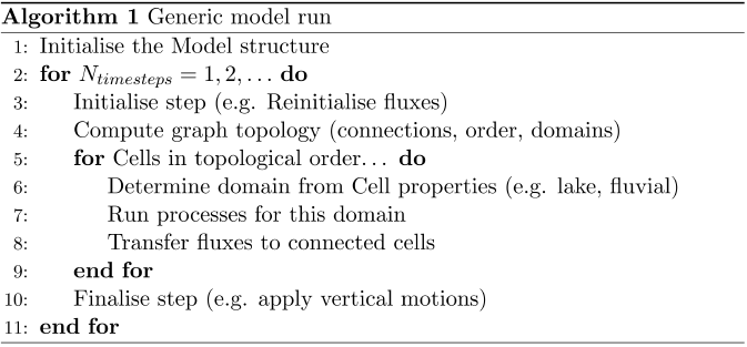
As illustrated in Fig. 2, the first step is to build the cellular structure by determining the fluxes and properties needed. These can be spatial data (e.g. precipitations, elevation, sediment provenance in stratigraphy), fluxes (e.g. fluvial sediments, water) or process parameters (e.g. erodibility). The second step defines the processes, i.e. the laws defining the interactions between all the fluxes and processes (e.g. fluvial incision, hillslope diffusion). Processes and/or fluxes can be domain-specific (e.g. marine, fluvial, lake, glacier). Finally, a graph structure providing the order of processing for the nodes needs to be determined. The graph structure has to be process-agnostic and capable of acknowledging domains of different topology. Algorithm 1 presents a simplified simulation.

An ideal numerical implementation of this principle should numerically separate fluxes, properties, processes and graphs. While complicated, numerical designs such as loose coupling can achieve this and ensure the different elements of the framework do not require presence or awareness of the others. In other words, it enables the addition, replacement or removal of processes affecting the same fluxes without needing to modify the rest of the model. For example, the model could change from a regular grid to a 1D profile or a Voronoi grid by simply “switching” the graph module. Some existing frameworks (e.g. Barnhart et al., 2020; Bovy, 2019) follow similar numerical design, but not in a cellular referential as we advocate in this contribution.

3.2 Building a directed acyclic graph

The first step consists in building a graph of connectivity on the landscape in order to determine a processing order for the cells that takes into account the topography of endorheic basins. Here, we use a regular rectangular grid to discretize topographic elevation, z. Each individual location, i, is a node from the point of view of the graph and holds a cellular automata cell. Each cell is connected to adjacent neighbours with the D8 direction, i.e. encompassing all the cells in diagonals and side directions. This defines the node graph, where for any given cell i we call all the connected cells with lower z receivers r_i and all the connected cells with higher z donors d_i. Cells with no donors are referred to as “source cells” while cells with no receivers are “pits” (if internal) or “edges” (if located on a matrix boundary). We implemented two types of boundary conditions at the edges: (i) open boundaries, where fluxes can escape the model and cells have no receivers, and (ii) periodic boundaries, where the fluxes communicate with the opposite cells (e.g. a cell at the eastern boundary is linked to its opposite at the western boundary). The graph hence created is a directed acyclic graph (DAG): each cell is linked to one or several receivers and cannot cycle back to itself. In graph theory, setting up a DAG allows for the use of a wide range of dedicated algorithms for topological ordering or graph traversals. The type of flow emulated by this DAG is called a “multiple flow direction” (Schwanghart and Scherler, 2014) as one cell can be linked to multiple receivers.

Note that the case of numerically flat surfaces, i.e. a node surrounded by others with the exact same elevation at numerical precision, needs particular care. In such situations, neighbours of i can end up being neither a receiver nor a donor and can generate cycles. Methods exist to process the flat surfaces (e.g. Barnes et al., 2014a). We use the carving algorithm by Cordonnier et al. (2019) to approximate an acyclic flow direction on these flat surfaces; the algorithm is detailed in the next subsection.

3.3 Computing a depression-aware topological order

Once the connection between cells is established – i.e. the receivers and donors of each cell are determined by the topography or by the rerouting algorithm on flat surfaces – we compute the topological order. It is a crucial step for any LEM: it determines the order in which cells need to be processed starting from the source nodes and finishing with the model edges. Alternative methods exist: it is possible, for example to utilize an iterative method accumulating fluxes progressively (e.g. Braun and Sambridge, 1997); solving large sparse matrices (e.g. Perron, 2011); using priority queue data structures to traverse the graph of cells dynamically (e.g. Barnes et al., 2014b, 2020).

Our implementation of an algorithm calculating a lake-aware topological order needs to satisfy a number of conditions: (i) conservation of the original topography of the depression in order to take its characteristics into account, and (ii) respect of the notion of upstream and downstream including potential lake and depression systems. We implemented two different algorithms to incorporate local minima in the model. First, a topological order can “passively” reroute local minima and approximate the flow path as if depressions were recognized but assumed to be entirely filled up to the elevation of the outlet. Second, an algorithm accounts for the volume of potential lakes, and uses separate dedicated processes within them. Both of the algorithms modify the DAG in order to emulate a notion of upstream/downstream by linking the pit nodes of the different depressions to an adequate outlet node. Finally, we apply a topological sorting algorithm on the modified DAG to calculate the depression-aware topological order.

We use the same topological sorting algorithm to calculate the topological order for both scenarios (detailed in Sect. 3.3.1 and 3.3.2). The algorithm is a modified implementation of the one in fastscape (Bovy, 2019) and very similar to the one described by Anand et al. (2020). It is O(n) in complexity, with n being the total number of links between the cells and their receivers in the graph. In short, a queue is initialized with the source cells. In turn, these are popped out of the queue, pushed into a stack array and their receivers are visited. An array tracks the number of times each cell is visited. If the number of visits equals the number of donors of a given node, it is saved into the stack and the process continues. Once the queue is emptied, all the cells have come through and the stack array contains all the node indices ordered. This stack array can be traversed in normal or reverse order to respectively process upstream or downstream cells first and is illustrated in Fig. 3. This process is equivalent to the steepest descent alternative of Braun and Willett (2013).

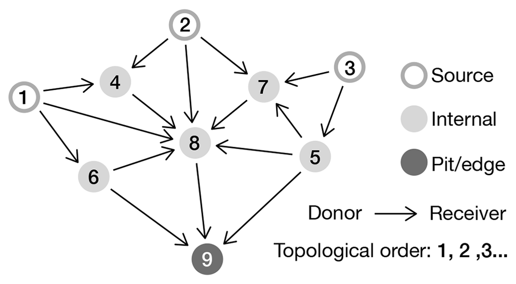
Figure 3 DAG topology, illustrating the relationship between the different nodes in the graph (cell location). The arrows depict individual relationships between a donor and one of its receivers. Node 9 is a pit, or local minima, if located inside the model grid and an edge if fluxes can escape from it. The topological ordering goes from the first node to be processed, to the last. Sources are nodes without donors.

3.3.1 Topological order for landscapes with passive lakes

The solver for passive lakes is designed for cases where depressions are a secondary feature of the landscape evolution study. It ensures flow continuity through the landscape and conservation of original topography by connecting the pit of each depression to an outlet that will eventually reach the model edge (Cordonnier et al., 2019). The solver bypasses the computational expense of considering the exact geometry of the depressions while still accounting for their existence. Our method is adapted from the work of Cordonnier et al. (2019), where the steepest descent graphs reroute local minima towards model edges. We only modify it to be compatible with multiple flow directions. The algorithm first links every node to either a single edge or a pit using a steepest descent route to define basins. It then links pairs of adjacent drainage basins using their lowest connections from the most internal to the most external one. This defines a receiver cell for the internal pit of each internal basin in order to ultimately drain to the edge.

Our implementation adds a couple of extra steps. First, our algorithm actually carves the surface in the case of flat surfaces in order to avoid 0-slopes (see Algorithm 3 in Cordonnier et al. (2019) which inverts the node-to-node steepest descent connections from the sill to the pit). We make sure to reassess all the potential multiple-flow links impacted by this single-flow rerouting (e.g. cells from the target basin partly flowing to the source basin). After this step, the topological order can be computed and will route flow through depression.

This method has the advantage of speed, versatility and stability as demonstrated by the benchmarks of Cordonnier et al. (2019). However, the links between basins are estimated with a steepest descent algorithm, which might shift the location of the geometrical outlet of the depression by a few pixels. It also maintains unconditional connectivity between local minima and their outlets, ignoring endorheism.

3.3.2 Topological order for depression-aware simulations

The depression-aware solver fully embraces the topographic complexity of depression systems. It does not assume the lakes outflow and treats them as separate domains. The geometry of depression systems can be convoluted with multiple levels of sub-depressions (Fig. 4). To deal with this complexity, we build a binary trees for each depression system with a principle adapted from Barnes et al. (2020): each vertex of the binary tree can only have up to two children, one parent and one twin. It is built with a “vertical” logic illustrated in Fig. 4 where each vertex corresponds to a spatially identifiable domain made of a single or multiple merged depressions. Building such trees ensures efficient operations to numerically navigate through individual depression systems (Barnes et al., 2020). We refer to the work of Barnes et al. for a detailed description of this binary tree and how to efficiently build it. This data structure has been utilized for flooding landscapes with finite amount of water (Barnes et al., 2021).

Our implementation differs from Barnes et al. (2020) for a couple of important points. For this contribution, the binary tree needs to be fully integrated within the topographic graph in order to enable topological sorting and downstream traversals. We therefore sacrificed some of the computational efficiency (in terms of memory and CPU) to store more information for communication between the topographic DAG and the binary trees of depression. Barnes et al. (2020) build a forest of binary trees connected to each other and to the “ocean” that Barnes et al. (2021) use to iteratively flood the landscape from one depression to another. Water flows through the whole landscape to the depression bottom and is then redistributed from one depression to another until all the water is used or all depressions are filled. Instead, we build independent local trees that are only connected to their surrounding DAG. Numerically, we only label nodes belonging to a depression inside the corresponding depression system instead of labelling and linking all nodes across the landscape to a depression like Barnes et al. (2020). We also store a lot of information on a cell basis, for example which cell belongs to which depression sorted by elevation. We opted for this heavier solution because, contrary to Barnes et al. (2021), we do not fill the depressions iteratively and only visit each cell once, as explained in Sect. 2.3. The most significant difference is perhaps the flow topology: we built CHONK to be compatible with multiple flow directions while the Barnes et al. (2020) and Barnes et al. (2021) counterparts are single-flow oriented. Thus a depression system can be linked to multiple others, whereby a steepest descent route can only link one depression system to another at a time. This point makes our algorithm significantly more convoluted, especially in the presence of complex systems of nested depressions (e.g. white noise). We note that all these modifications added to fit our needs complicate the original algorithm and can make it significantly slower in many cases. We are not presenting a version with better computing speed or accuracy compared to the work of Barnes et al. (2020) and Barnes et al. (2021). We adapt its use to our prototype to explore the consequences of explicitly considering lakes in LEMs. A cleaner, performance-oriented solution could benefit from being entirely based on Barnes et al. (2020) and Barnes et al. (2021); however, using their version out of the box would require significant work to achieve all the features we need for CHONK.

We make heavy use of priority queue-based algorithms to build the graph (see Barnes et al., 2014a and Barnes et al., 2020 for full details about this data structure). This enables the dynamic sorting of selected cells as a function of their elevation. First, we place each internal pit cell in individual priority queues as a starting point for all the base depressions and we label the cell with a unique depression ID (black dots in Fig. 4a). We process each priority queue until it is empty by popping out the lowest elevation cell and checking all of its neighbours. If the neighbour is higher in elevation, it is placed in the queue for later processing or labelling. This process runs until the cell being processed is already labelled as belonging to another depression. In this case both are registered as twins. Each twin records the connecting cell as their tipping node (e.g. depression 2 and 3 in Fig. 4a). If one of the neighbours has a lower elevation, that cell is labelled as outlet and this depression is placed at the top of its tree – or remains an outlet as long as it is not labelled as a twin by another priority queue. The trees are complete once all priority queues are empty. Note that while we do not detail each and every one of them for the sake of conciseness, the algorithm needs to potentially manage a lot of specific edge cases.

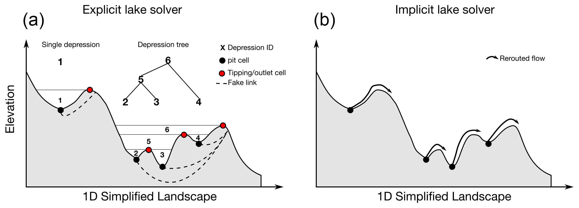
Figure 4 (a) Cartoon illustrating the depression tree structure on a simplified 1D landscape. Each depression system has its own sub-tree, which can be as simple as a single depression (e.g. depression 1). Dotted arrows represent fake temporary links used by the model to calculate an upstream/downstream direction despite the complex topography – the sole elevation value not being relevant in the case of local minima. (b) Illustration of the lake solver for passive simulations which reroutes flow using Cordonnier et al. (2019). Note how the flow is rerouted unconditionally to a model edge following a minimal cost path based on the elevation of the connections between each watershed and the direct connection to the edge. For both (a) and (b) the landscape is represented in a simple 1D section. In 2D the problem becomes increasingly convoluted, especially if low-level noise or flat surfaces pollute the elevation.

The data structure allows us to process the following metrics for each depression:

• a depression level, which represents the maximum distance in the tree from a base depression. Each base depression is at level 0, and each parent's level is equal to the maximum level of their children plus 1,

• the minimum volume of a depression (0 if base depression, the minimum volume to fill all the children and “reach” the depression in the tree),

• the volume of the depression V_total if filled, note that it includes the volume of their children if any,

• the maximum elevation of the depression if filled,

• the tipping node of the depression, which represents either the outlet of the whole subsystem, or the node joining two twins.

In addition to the depression-specific information, the model stores a number of internal structures to navigate between the topographic graph and the depression tree. Note that the maximum volume of water can account for potential evaporation if it is enabled in the model.

Our depression tree relies on the principle of uniqueness of the tipping points which can be invalidated by numerically flat surfaces or if depression borders have equal elevation. To prevent this, we add minute numerical noise between $-{\mathrm{10}}^{-\mathrm{6}}$ and 10⁻⁶ m at each time step and carve depressions with insignificant volumes using Algorithm 3 of Cordonnier et al. (2019).

After building the depression tree, we can finally calculate the topological order for the depression-aware lake solver. This is achieved in the DAG by temporarily linking the pit cell of each base depression to the cells that lie downstream of the outlet of the above depression in each system (Fig. 4a). These links ensure that any lake system will be processed before its downstream counterparts and is cancelled after the calculation of a topological order.

3.4 Cellular automata structure

3.4.1 Properties, parameterization and tracking

Once the DAG is built, the model skeleton is ready and a cell is attributed to each node. The information held by each cell can be adjusted and expanded on a needs basis. In the current implementation, cells have the following properties updated at each time step (illustrated in Fig. 2):

• topographic elevation (in m)

• thickness of the immobile sediment layer (in m)

• volumetric water flux Q_w in m³ yr⁻¹ traversing the cell

• volumetric sediment flux Q_s in m³ yr⁻¹ traversing the cell (mobile sediments)

• proportion of sediment flux from the river or the hillslope systems

• a list of the downstream cells receiving either sediment or water in transit, calculated from the graph and from the process law implemented in the model

• lists of weights describing the proportions of sediment and water transmitted to each downstream receiving cell

• erosion, sediment entrainment and deposition fluxes

• tracking information if activated (e.g. proportion of the sediment flux coming from a given source area).

Three kinds of parameter inputs are currently available. First, external parameters which can be single values (e.g. dx, dy, dt), or global arrays (e.g. 2D matrices of precipitation or uplift), varying in space and/or time. Second, parameters that are label-dependent: a 2D matrix of labels defines discrete spatial areas and each label has a set of distinct parameters, for example different rock type can be associated with different erodibility and diffusivity (Gailleton, 2021). And third, parameters that are fully dynamic: they are interdependent of each other and defined by a function rather than a given value. Examples of the latter are detailed in Sect. 4.4.

The tracking capabilities of the method also rely on the labels. While the numerical implementation is tedious, its principle is simple and powerful: any material eroded by any process from any location keeps track of its label when it is incorporated in the mobile sediment flux. The mobile sediment flux is partitioned to the receivers alongside the water flux, adjusted for local erosion and deposition processes. In the stratigraphy, a dynamic sparse matrix of cells stacks “containers” of sediments and keeps track of label proportions to guarantee tracking if re-eroded.

It is worth noting, however, that this cellular automata structure has some numerical limitations. To maintain all the advances detailed in this contribution, all the calculations need to be processed from ridge to outlet, which is not necessarily compatible with all numerical laws. For example, solving stream power-like equations implicitly necessitates multiple graph traversals in the upstream and downstream directions, therefore limiting the amount of upstream information a cell can use in the processes (e.g. Braun and Willett, 2013; Campforts et al., 2017; Hergarten, 2020). However, they are not fully incompatible: one could imagine calculating a “static” erosion field with one of these implicit schemes and post-process them using the cellular automata method to integrate upstream information (e.g. provenance), only sacrificing the dynamic adjustment capabilities.

3.4.2 Cell-processing order for local minima

The model processes the cells following the upstream-to-downstream topological order first assuming that there are no lakes. Before their turn, unprocessed cells receive water and sediments from upstream neighbours. When a cell is next in the topological order, the model applies external flux modifiers on it: precipitation, infiltration or any related process law affecting the water or sediment flux by addition or removal from external sources. Then the process laws affecting the cell are executed in the following order: water routing; fluvial incision, deposition and sediment entrainment; and/or hillslope diffusion following equations described in Sect. 4.1. At that stage, the model calculates weights for the distribution of sediment and water across the cell receivers. Finally, transport processes transmit water and sediment to the unprocessed receiver cells, along with the proportion of sediment fluxes respectively belonging to hillslope and fluvial domains.

When the solver for passive lakes is activated, cells in the area affected by the local minima are processed like any other cells. However, flow is rerouted from the pit cell to the lake outlet and this effectively reduces the topographic gradient, enhances deposition processes, and reduces erosion processes.

Solving lakes is done in multiple steps. Cells are processed normally, i.e. with fluvial and hillslope processes, following the downstream topological order. By definition, all the pit cells of a given depression system are processed before any section of the landscapes downstream of the lake. If the processed pit cell is the last of its depression system (in the case of a simple lake there is only one pit, but nested depression systems can have multiple pits) we can use the full volume of sediment and water in these cells to fill the lake(s) using the pre-computed depression trees.

The first step consists in calculating the total amount of water entering the full depression system by summing Q_w for each pit node of base depressions in the system. The tree is traversed from bottom to top, propagating the water from children to parents. In the end, the following volume of water V_{w in} enters each depression:

$$\begin{array}{}\text{(1)}& V_{\text{w in}}=\sum _{i_{\mathrm{pit}}}{Q}_{\mathrm{w}}\mathrm{\Delta }t,\end{array}$$

where i_pit is the cell index of every pit cell downstream of a given depression.

The second step determines whether the depression system needs breaking into sub-trees: the full tree is assessed from the top depression down. If the sum of available water is more than what the top depression can store, the whole lake system fills with water and will outflow. Otherwise if the minimum amount of water storable in the top depression is less than V_{w in}, the lake does not outflow but all the child depressions will be filled. Finally, if the minimum amount of water storable in the top depression is greater than V_{w in}, the local tree is divided in two and the assessment is reiterated until all the sub-trees are filled. Note that all the water entering can also evaporate, in which case no lake is created.

The third step consists in calculating the elevation of the lake (z_w). Because our current implementation solves explicit finite difference schemes, we assume that, within a time step, the volume of water in the lake solely determines z_w. Elevation changes due to lake sediment deposition are only applied at the end of the time step. If the lake outflows, h_w equals the elevation of the outlet cell. Underfilled depressions lead to more complications (Garcia-Castellanos and Jiménez-Munt, 2015). In these cases, the model calculates a balance between lake evaporation and the available amount of water. Using a priority-queue-based graph traversal (see Sect. 3.3.2), we traverse the depression cells in increasing elevation order. Cells are included one by one and contribute in turn to storing the available amount of water V_{w avail} while giving their elevation to h_w:

$$\begin{array}{}\text{(2)}& V_{\text{w avail.}}=V_{\text{w avail.}}-N_{\mathrm{lake}}\mathrm{d}x\mathrm{d}y(\mathrm{\Delta }z+Q_{\text{w evap}}),\end{array}$$

where N_lake tracks the number of cells already in the lake, Q_evap is water lost to evaporation, and Δz the elevation difference between the current h_w and the elevation of the next node in the priority queue. The final h_w is calculated once $V_{\text{w avail.}}<N_{\mathrm{lake}}\mathrm{d}x\mathrm{d}y(\mathrm{\Delta }z+Q_{\mathrm{evap}})$.

3.4.3 Water and sediment fluxes into and across lakes

Once the water elevation is determined, the model back-calculates sediments. All the cells below water are “deprocessed” from continental processes: fluvial and hillslope processes are reversed with adequate correction on cells sediments and water contents. The volume of sediment stored in the lake, V_{w evap}, can now be stored in the lake in a straightforward manner as its final volume is known. Any excess is transmitted to the outlet cell. As noted by Garcia-Castellanos (2006) and Garcia-Castellanos and Jiménez-Munt (2015), the outlet of the lake needs particular care as its behaviour through time ultimately controls its draining. The de-processing of the outlet is only partial as it gives sediments to the lake and to the downstream landscape. Only the part of the fluxes going into the lake needs to be cancelled and the other parts need to be recalculated with the new amount of sediment and water. The latter are determined by subtracting the incoming V_w and V_s by what has been stored. Additional care is needed to consider water and sediment coming to the outlet from its non-lacustrine upstream neighbours.

We cannot stress enough how convoluted this de-processing can be, numerically speaking. One needs to account carefully for all the neighbouring cells of the outlet and not remove/re-add fluxes multiple times. Given the critical nature of this task, we make sure our model is not plagued by uncovered edge cases and we implemented mass-balance checkers making sure no water or sediments are lost due to the transfer processes. Mass-balance for a transferable flux can simply be defined as follows:

$$\begin{array}{}\text{(3)}& M=Q_{\mathrm{in}}-Q_{\mathrm{out},}\end{array}$$

where Q_in encompasses any fluxes being added to the system and Q_out any fluxes leaving the system. For water flux, Q_{w in} includes effective precipitation as well any water stored in a lake at the previous time step (when using the depression-aware lake solver). Q_{w out} encompasses any water stored in a lake at the current time step, evaporation and water leaving the system via the model edges. For sediment fluxes, Q_{w evap} includes any process eroding material and putting it in transported flux (e.g. incision, entrainment, diffusion) and Q_{s out} any processes depositing sediment from this flux (e.g. fluvial deposition, lake deposition) or exiting the model via the edges. The mass balance is respected if M=0 (plus or minus numerical precision errors). Note that a simpler alternative would be to process the water fluxes separately to avoid the de-processing. However, this contribution aims to develop a method able to keep unconditional interoperability between all the fluxes and processes, which would be broken by such sequential separation.

Finally, once all cells have been processed, each cell updates the topography and the sediment layer with its erosion and deposition fields. The model also calculates and formats data to monitor the direct model outputs (e.g. maps of erosion, water fluxes, sediment thickness) and indirect outputs such as the sum of the sediment fluxes outletting the model versus the sum of sediment fluxes stored in sediment layers.

4 Application of the framework to new challenging scenarios

We demonstrate the capabilities of the method with three fields of applications. First we test the effect of considering lakes in a tectonically active range with an internal basin. We then illustrate the tracking capabilities of the model by monitoring the sediments flux coming from a magmatic pluton. Finally, we explore the dynamic parametrization feature with the previous pluton settings, and adapt parameters in function of sediment flux composition. All the models start from the same near-steady-state landscape obtained after running a simulation until drainage stabilization with block uplift and non-subsiding foreland. The model has been tested on a computer with an Intel i9-10980HK and 32 GB or RAM on both MacOS 11.7, Windows 10 and Linux Ubuntu 22.04.

4.1 Process laws

To test the framework, we implemented a set of process laws that simulate long-term hydrology, fluvial, and hillslope processes.

4.1.1 Hydrology

Hydrology in long-term LEMs is usually approximated by a flow-routing algorithm distributing weighted drainage area from source nodes to outlets in the downstream direction. The weights represent the spatial variation of precipitation rates (see Leonard and Whipple, 2021, for a comprehensive review on the subject). First, the local effective precipitation is added to the water discharge in the considered cell i:

$$\begin{array}{}\text{(4)}& Q_{i\mathrm{w}}=Q_{i\mathrm{w}}+P_i\mathrm{d}x\mathrm{d}y,\end{array}$$

where P_i is the local effective precipitation weight factor that can include infiltration.

The second step is the routing to receivers. It can follow the steepest descent single-flow direction (e.g. O'Callaghan and Mark, 1984; Braun and Willett, 2013) or a multiple-flow direction (e.g. Tarboton, 1997; Schwanghart and Heckmann, 2012; Armitage, 2019). We implemented an adaptive algorithm routing water with multiple flow following the method of Bovy (2019). We added an optional parameter to enable dynamic switching to single-flow routing after an arbitrary threshold of discharge, in order to roughly simulate a transition from hillslope to fluvial domains. Note that we use relatively large cell sizes (dx=200 m) and this parameter is optional. In the multiple-flow domain, water is split according to the local slope. Following Bovy (2019), an exponent p_r is calculated for each receiver r of a cell i:

$$\begin{array}{}\text{(5)}& p_{\mathrm{r}}=\mathrm{0.5}+\mathrm{0.6}{\displaystyle \frac{\mathrm{d}z}{\mathrm{d}x}},\end{array}$$

and then normalized to satisfy $\sum p_{\mathrm{r}}=\mathrm{1}$ and conserve mass balance. The water flux is then transmitted to each receiver with

$$\begin{array}{}\text{(6)}& Q_{\mathrm{w}}=Q_{\mathrm{w}}+Q_{i\mathrm{w}}^{p_{\mathrm{r}}}.\end{array}$$

4.1.2 Fluvial erosion and deposition

We simulate fluvial erosion and deposition using the SPACE model (Shobe et al., 2017), a hybrid law allowing for simultaneous treatment of the detachment-limited and transport-limited portion of the rivers based on Davy and Lague (2009). SPACE can process all kinds of landscapes, whether sediments are absent or they saturate the system. The process law separates sediment entrainment ^fE_s, bedrock incision ^fE_r and sediment deposition ^fD_s into three equations solved simultaneously:

$$\begin{array}{}\text{(7)}& {\displaystyle }{E}_{\mathrm{s}}=K_{\mathrm{s}}{Q}_{\mathrm{w}}^m{S}^n\left(\mathrm{1}-e^{-\frac{H}{H^{*}}}\right),\text{(8)}& {\displaystyle }{E}_{\mathrm{r}}=K_{\mathrm{r}}{Q}_{\mathrm{w}}^m{S}^n{e}^{-\frac{H}{H^{*}}},\text{and}\text{(9)}& {\displaystyle }{D}_{\mathrm{s}}=V{\displaystyle \frac{Q_{\mathrm{s}}}{Q_{\mathrm{w}}}},\end{array}$$

where K_s is the sediment entrainment coefficient regulating the ease with which sediment cover can be mobilized; K_r is the erodibility coefficient ultimately controlling local rock strength (proxying various factors such as weathering or fracturing); m and n are exponents regulating the relative importance of topographic gradient and water flux in the stream power law (e.g. Harel et al., 2016); H is the sediment height; H^* is the bed roughness index linked to the proportion of bedrock not covered by sediment; V is a dimensionless settling velocity coefficient encompassing information about the turbulence and composition of the suspended load. Details on all these parameters can be found in the original paper by Shobe et al. (2017). In the case of multiple flow departing from a single cell, the process is simply summed for each receiver: S, Q_w and Q_s being different for each one.

4.1.3 Hillslope diffusion

Following the same philosophy, we implemented the non-linear hillslope diffusion of Carretier et al. (2016). This law separates sediment entrainment from deposition (i) enabling greater numerical stability than the purely non-linear explicit scheme (Roering et al., 1999) while (ii) keeping the non-local, non-linear aspect of the diffusion process. This law is versatile and collapses to both linear and non-linear end members under different contexts as demonstrated in Carretier et al. (2016). Material entrainment follows a local, straightforward linear diffusion scheme which is defined as

$$\begin{array}{}\text{(10)}& {\displaystyle }{E}_{\mathrm{rock}}={\mathit{\kappa }}_{\mathrm{rock}}{\displaystyle \frac{\mathrm{d}z}{\mathrm{d}x}},\text{(11)}& {\displaystyle }{E}_{\mathrm{soil}}={\mathit{\kappa }}_{\mathrm{soil}}{\displaystyle \frac{\mathrm{d}z}{\mathrm{d}x}},\end{array}$$

where E_rock and E_soil are the entrainment rate in [L T⁻¹] for bedrock and sediment respectively; and κ_rock and κ_soil are modulating parameters as a function of the physical characteristic of the substrate and soil. Note that it is possible to disable bedrock diffusion to consider soil movements. In the case of multiple flow, we respect the numerical implementation of Carretier et al. (2016) considering that the steepest slope is the main driver to calculate $\frac{\mathrm{d}z}{\mathrm{d}x}$. If both E_rock and E_soil are active, E_soil is applied first. If E_soil×dt is greater than the soil thickness, the remaining E_rock is applied proportionally to the remaining fraction of bedrock. For example, if $E_{\mathrm{soil}}\times \mathrm{d}t=\mathrm{0.2}$ m but soil thickness is 0.1 m, then E_rock is applied at 50 %. Deposition of sediment by hillslope processes is non-local and relies on a transport length approach based on Davy and Lague (2009):

$$\begin{array}{}\text{(12)}& {\displaystyle }{D}_{\mathrm{hill}}={\displaystyle \frac{Q_{\mathrm{s}}}{L}},\text{where}\text{(13)}& {\displaystyle }L={\displaystyle \frac{\mathrm{d}x\mathrm{d}y}{\mathrm{1}-{\left(\left(\frac{\mathrm{d}z}{\mathrm{d}x}\right)/S_{\mathrm{c}}\right)}^{\mathrm{2}}}},\end{array}$$

where S_c is a critical slope parameter (Roering et al., 1999). If $\mathrm{d}z/\mathrm{d}x\ll S_{\mathrm{c}}$, most of the sediments are deposited and we approach the linear side of the equation. When $\mathrm{d}z/\mathrm{d}x\to S_{\mathrm{c}}$, most of the sediments go to the receivers as predicted by the non-linear diffusion. In the case of $(\mathrm{d}z/\mathrm{d}x)>S_{\mathrm{c}}$, the process recasts the slope to S_c, adding any excess material to Q_s. A conceptual difference with Carretier et al. (2016) is that we express volumetric flux rather than flux by unit width. This does not affect the physical behaviour of the process but is more consistent with the rest of our implementation. Q_s is modified according to E_rock, E_soil and D_hill and fluxes are distributed to multiple receivers proportionally to the slope.

4.1.4 K and κ coefficients for erosion and sediment transport

The coefficients for hillslope and fluvial erosion or sediment transport – κ_s, κ_r, K_r and K_s – are empirical and their value can greatly vary from one site to another (e.g. Harel et al., 2016; Carretier et al., 2016). In stream-power-like models, they are roughly a function of m, n and local conditions. In hillslope diffusion, they are a function of local soil and lithologically driven heterogeneity (Carretier et al., 2018). Because both of these empirical coefficients encompass many processes (e.g. Tucker and Slingerland, 1996; Whipple et al., 2013), we use a common base value for each parameter across the whole landscape, or parts of it. These values can be modulated by local or global heterogeneities. The base values can be estimated with sensitivity analyses of spatially variable weighting coefficients and obtain relevant elevations.

4.1.5 Lacustrine sedimentation

Lake deposition is approximated with a simple draping algorithm. Once the final state of a lake is known (see Sect. 3.3), we calculate the proportion of the lake that can be filled with incoming sediment in each pixel: $V_{\mathrm{slake}}/\left(V_{\mathrm{totlake}}{h}_{\mathrm{lake}}\right)$. While simplistic, it serves the purpose of this contribution to be a proof of concept in treating lakes as separate entities and paves the way to more detailed lacustrine processes.

Table 1 Parameters for the different simulations

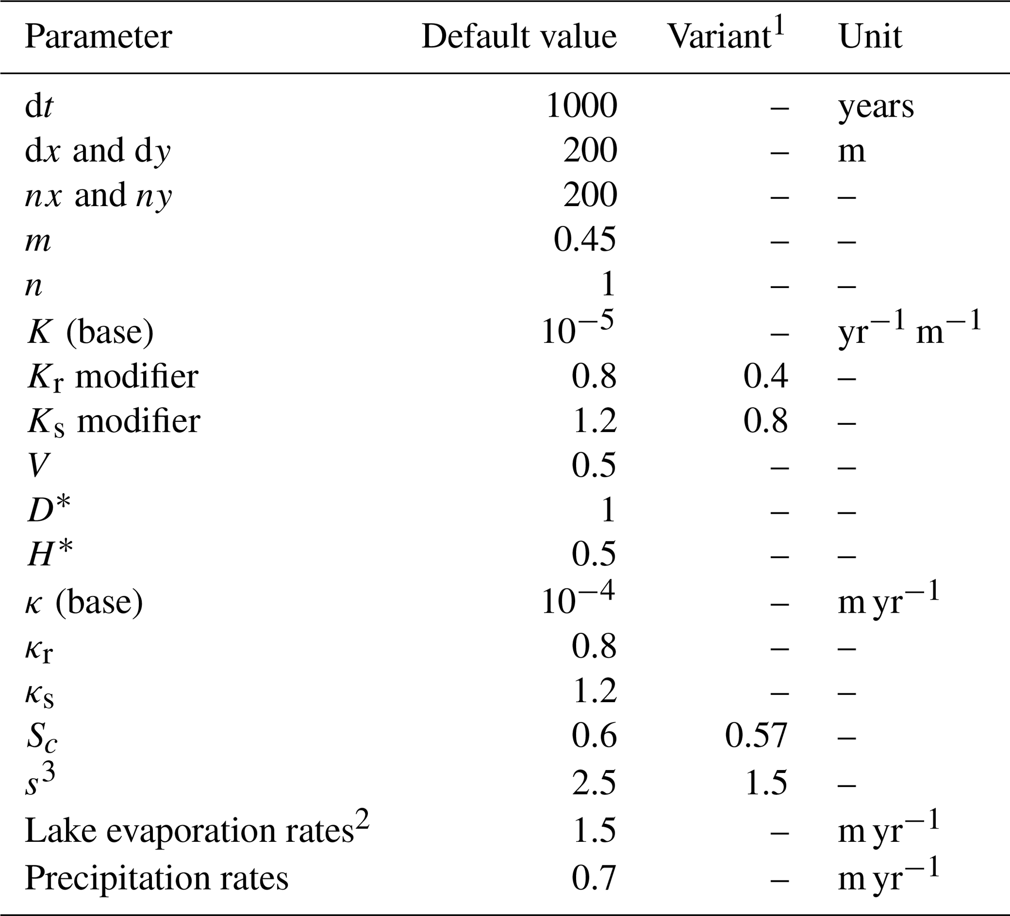
¹ For the scenarios with another rock type. ² Only for scenario 2c. ³ Only for scenario 3b.

4.2 Application I: considering lakes in long-term landscape evolution

In this first set of experiments, we assess the role of lakes and closed basins in long-term landscape evolution. Earlier work by Garcia-Castellanos (2006) and Garcia-Castellanos and Jiménez-Munt (2015) (1D and 2D respectively) already noted that endorheism in LEMs was a function of complex relationships between climate (precipitation, evaporation), tectonics and surface processes. Their experiments highlighted the potential importance of integrating endorheism in long-term and large-scale landscape evolution studies. Here, we exploit our the capacity of our method to process lakes in order to assess how it could impact simulation results for a given setting.

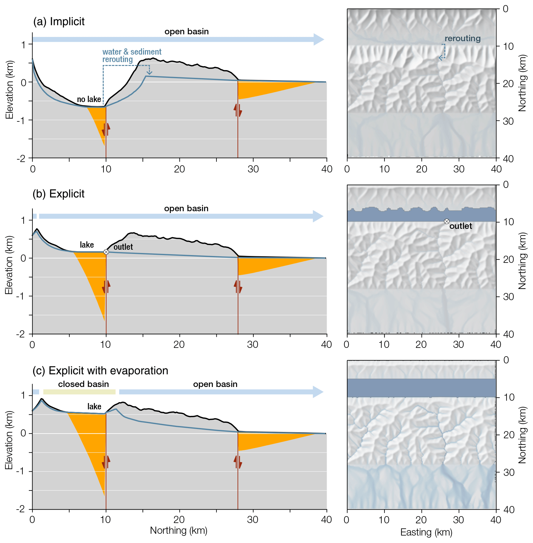
Figure 5 Resulting landscapes after 5 Myr simulation for scenarios 1, 2a and 2b in (a), (b) and (c). The left column displays N–S cross sections of the median (black line) and minimum elevation (thin blue line) and the median sediment height (filled area in orange). The right column shows the extent of lakes (dark blue) and the water flux (blue) on a shaded topography. The minimum topography is a proxy for the elevation of the main river profiles, and highlights a drainage divide in (a) and (c). Parameter values can be found in Table 1.

We ran three simulations for 10 Myr in an idealized mountain range with a frontal thrust, a foreland, and a normal fault in its hinterland (Fig. 5). A uniform, semi-arid, yearly precipitation rate was set at 700 mm. Scenario 1 uses the passive lake solver (Sect. 3.3.1), scenario 2a runs with the depression-aware lake solver (Sect. 3.3.2) and scenario 2b has the depression-aware lake solver with lake evaporation. Figure 5 displays a snapshot of the landscape after 5 Myr as a N–S median profile of median and minimum elevation and median sediment thickness and a hillshaded map-view of Q_w and lake extents. Figure 6 shows time series of sediment fluxes escaping the southern border of the model as well as the total volume of deposited sediment over the landscapes.

In scenario 1, an unrealistically deep (−500 m after 5 Myr), underfilled and subsiding basin has formed on the footwall of the normal fault. The main E–W drainage divide migrates significantly to the south (Fig. 5a). Over a total 10 Myr long evolution, the two basins store 4×10¹¹ m³ of sediments while the exported sediment flux is only mildly impacted by the onset of the normal fault (Fig. 6) and shows steady increase after 2 Myr. In scenario 2a, using a depression-aware lake solver, sedimentation in the internal basin balances off subsidence. A long-lived very shallow lake is continuously connected to the foreland via a single river (Fig. 5b). The sediment export through time initially is nearly halved from 4 to 2.5×10⁵ m³ yrs⁻¹ as the depression grows and stabilizes beyond 3 Myr (Fig. 6). Finally, in scenario 2b, a closed basin forms on the hanging wall of the normal fault (Fig. 5c). Its elevation increases through time and it traps all the incoming sediments and water. It quickly becomes disconnected from the foreland (Fig. 5c). The exported sediment flux is halved from 4 to 2×10⁵ m³ yr⁻¹, and increases again slightly and steadily through time (Fig. 6).

In scenario 1, the internal depression is unconditionally connected to the rest of the outlet by the passive lake solver and only fluvial deposition can fill the basin. The subsiding basin surface in Fig. 5a demonstrates fluvial deposition is not efficient enough to balance the subsidence. If the topographic signature of the normal fault is exaggerated, Fig. 6 shows that its sediment flux signature is greatly attenuated (minor drop for 2 Myr). More striking is the steady increase of sediment export, which can be explained by the constant lowering of the internal base level and the steepening of the internal basin. The steeper slopes erode faster and the ever greater volume of sediment is exported to the foreland due to the unconditional rerouting. Ultimately, if scenario 1 ran for longer it would display a meaningless landscape inversion draining to the depocenter of the internal basin and “teleporting” sediments to the model edge.

In scenario 2a, the lake almost constantly outflows, maintaining connectivity to the foreland the whole time. This is due to the large amount of water coming from the basin flanks compared to the accommodation space offered by the lake. The erosion of the outlet is barely impacted by the relatively small amount of water stored in the lake (this point is discussed in greater extent later in the Discussion). The balance between maintaining the connection to the foreland base level but maintaining the ability to trap sediment explains the stability of the basin elevation (Fig. 5b) and sediment export through time (Fig. 6) in equilibrium with the tectonic conditions. This results in very low actual lake depth (<1 m most of the time); however, this needs to be interpreted bearing in mind the time step of our simulation is 1000 years and represents an average of processes in that time span. In reality, this could be translated into patches of migrating but more realistically deep lakes. More sophisticated acknowledgement of lake sediment dynamics such as compaction could also enhance the creation of more realistic lakes (Håkanson, 1982).

Finally, scenario 2b is the only one breaking the connectivity to the rest of the landscapes, effectively simulating a closed basin. Lake evaporation balances water input in the lake and enables a decoupling where the would-be outlet of the lake does not receive any water or sediments from the lake, inhibiting its erosion compared to scenario 2a. The absence of outlet for the depression means all sediments are trapped within, explaining the highest volume of sediments stored and the lowest export to the model edges. The elevation of the overall model also rises, and if run for longer, the model would probably reach a steady state where the basin would be eventually captured by a river draining externally. The globally higher elevation and the increase of erosion export through time (Fig. 6) result from the increasing elevation of the internal basin and steepening of the landscape.

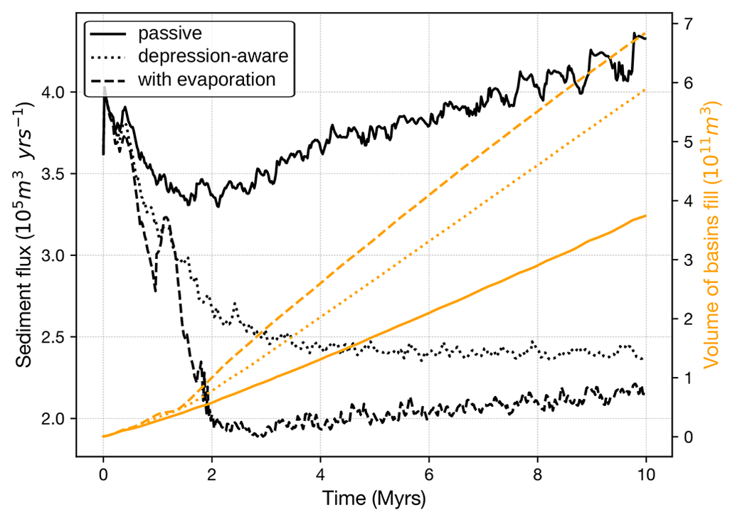
Figure 6 Sediment flux escaping the southern boundary of the model (black) and stored in the landscape (orange) for scenarios 1 (solid line), 2 (dotted line) and 3 (dashed line).

4.3 Application II: monitoring the source-to-sink system

This case demonstrates the ability of the CHONK framework to provide fine-grained detailed information about provenance in the stratigraphy. LEMs have been widely used to investigate the source-to-sink systems (e.g. Guerit et al., 2019; Yuan et al., 2019; Sharman et al., 2019). One particular need in this context is tracking the provenance and destination of material during their erosion, transport and sedimentation processes. This can be done by tracking discrete individual particles (Carretier et al., 2016), or with a bulk approach (Sharman et al., 2019). The latter usually post-processes this information by integrating the erosion and sedimentation field. Our approach enables an easy embedding of such information within the cell. Provenance tracking is built in and straightforward. Provenance can be tracked within the stratigraphy and reutilized in later time steps without information loss. We demonstrate the model capabilities with a run similar to scenario 2 from Sect. 4.2, but exhuming a simple pluton-like body of harder rock type in the range. Greater rock strength was simulated with a decrease in erodibility. We refer to the harder rock type as “granite” and the background rock type as “substrate” for simplicity.

We ran the simulation for 10 Myr. Figure 7a illustrates high-resolution monitoring of sediments with a granite provenance. Thanks to the 3D cellular system storing this information, it can be retrieved with different resolutions, for example in the full sediment column or in the first 10 m as illustrated in the left and right parts of Fig. 7a. Figure 7b and c display this information in cross-section views which highlight large-scale stratigraphic structures. Note that here, the provenance data are displayed as relative proportion instead of absolute volume, but both options are possible. The E–W and N–S cross sections in Fig. 7 illustrate the irregularity in the stratigraphic patterns of deposition as the distributary system sweeps across the foreland.

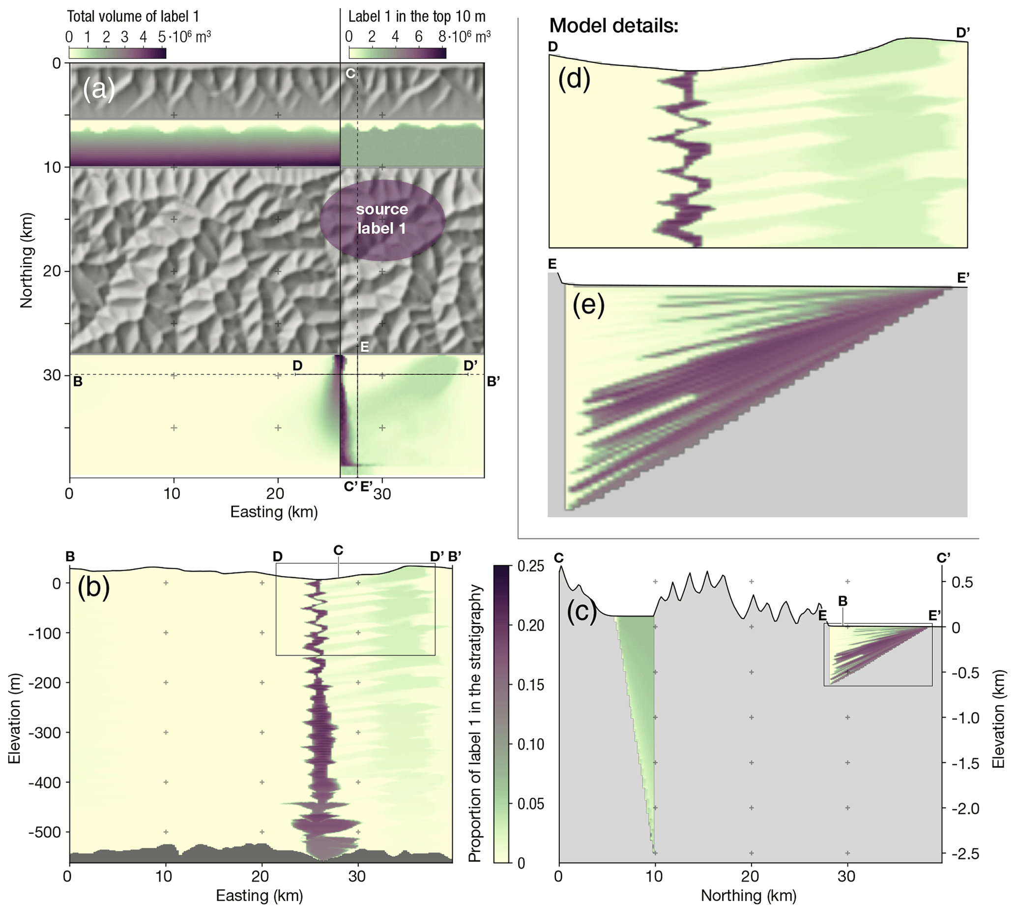
Figure 7 Illustration of the capabilities of CHONK to track the provenance of sediment fluxes through space and time. We simulated the exhumation of a pluton of more resistant rocks and tracked its evolution in the stratigraphy for 10 Myr. The colour scheme reflects the concentration of source material from light (low) to dark (high). (a) A map view of the source and distribution area of the material. The total volume of source material is shown in the entire stratigraphy (a, b) or its top 10 m (d, e, c). (b) A cross section of the foreland stratigraphy, illustrating the spread of source material through space and time. (c) A profile across the mountain range illustrating the relatively homogeneous internal basin versus the more complex foreland. (d) The avulsion patterns of (i) the main river (purple zigzags) and (ii) at higher extents a smaller tributary (light green). (e) Zoom-in on the foreland to detail the fan patterns evolving through time. Parameter values can be found in Table 1.

4.4 Application III: erosivity and erodibility captured by dynamic parameters

While the tracking capabilities open many options to monitor the source-to-sink system, they can also be used to integrate feedbacks between processes and characteristics of the sediment flux. Because tracking is dynamic, the state of the fluxes is always known and it can be used to directly influence the process laws. In the following example, we alter the K coefficients of erosion efficiency in Eqs. (9) and (7) to incorporate a notion of relative strengths between sediment and substrate. We assume that harder tools (e.g. granite) impacting softer bedrock (e.g. mudstone) yield greater river incision than softer tools (e.g. schist) on harder material (e.g. Sklar and Dietrich, 1998; Sklar, 2001; Sklar and Dietrich, 2004). We take advantage of the dynamic parametrization of CHONK to implement a first-order tool strength principle:

$$\begin{array}{}\text{(14)}& K_{\mathrm{eff}}={{\displaystyle \frac{K_{\mathrm{r}}}{K_{\mathrm{sed}}}}}^{\mathrm{s}}\times K_i,\end{array}$$

where K_eff is the effective erodibility used in the equation, K_r is the bedrock erodibility, K_sed is the erodibility of the mobile sediment, s is an exponent regulating the sensitivity of the system and K_i is the local erodibility factor. K_sed is a weighted average proportional to the content of each lithology in the model. We store the proportion of each lithology as detailed in Sect. 3.4.1. K_eff encompasses non-local effects that K_r and K_s cannot express. The latter are simply linked to the local condition of the cell and have no information about upstream conditions. This interdependence between the nature of non-local sediment flux and local erodibility would not be possible without an integrated approach like the one offered by CHONK.

We ran a modified simulation with an uplifting range and a static foreland, essentially Fig. 7a without the normal fault. We start from steady-state conditions and exhume a simplified granitoid. Figure 8 shows the profile of the main river draining through the granitoid at t=0 and t=3 Myr for an unmodified simulation using Eq. (9) and the tool effect simulation using Eq. (14) to highlight non-linear and non-local effects. The lower effective erodibility of the granite traversed by weaker bedload leads to a steeper stream. With hard tools enhancing incision, the slope of the area downstream of the harder rocks is reduced, which drops the base level and propagates knickpoints up all tributaries. Because this enhanced incision is a function of the quantity of granite in the mobile sediments, its effect fades downstream as more softer sediment is added in the mobile flux, affecting the concavity of the river profile non-linearly.

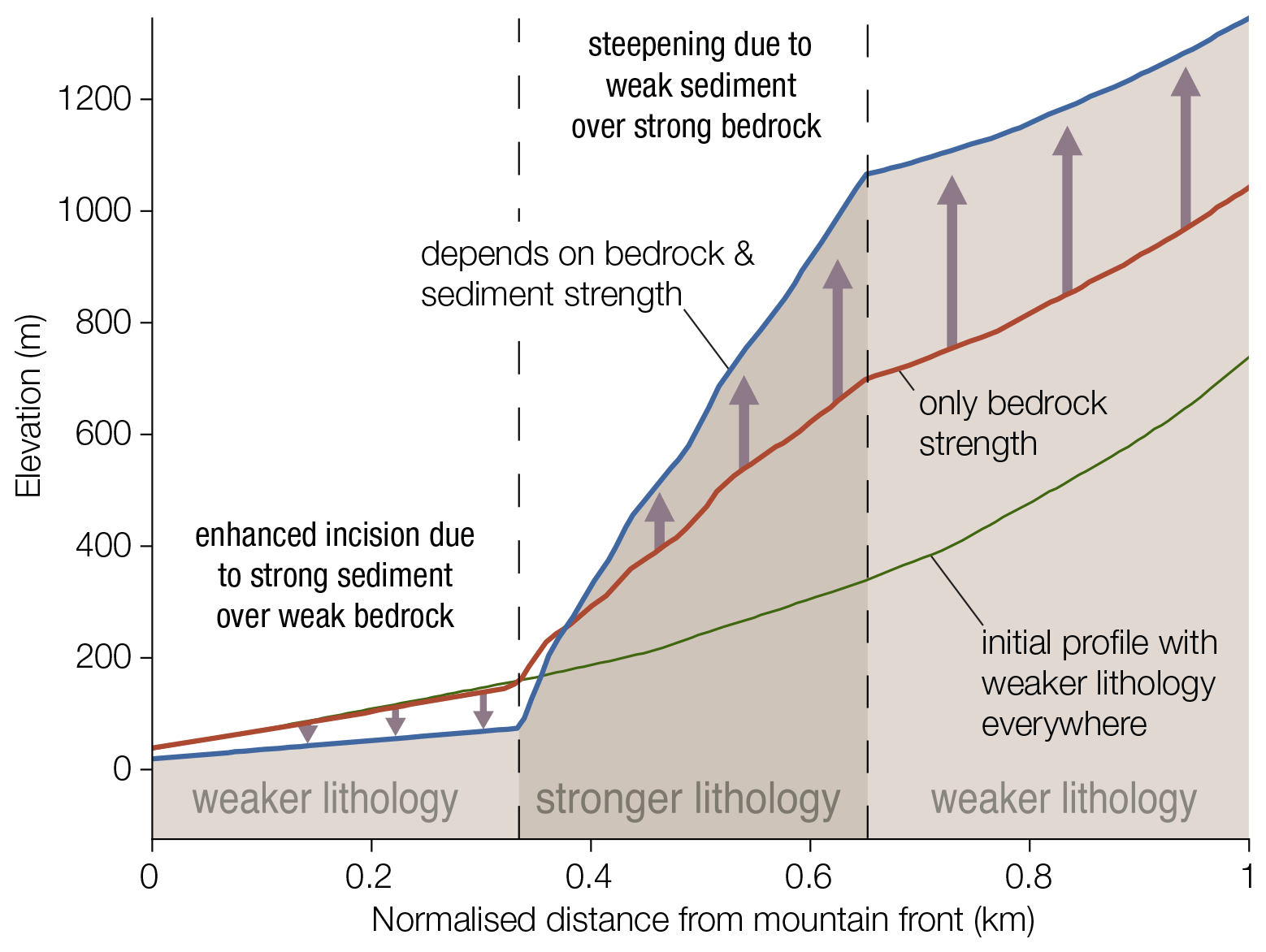
Figure 8 River long profiles normalized to mountain front for the initial topography (light green) and the simulation with and without the modified Eq. (14) (respectively in blue and red). The initial profile was near equilibrium with homogeneous lithology, hence is unaffected by the modified equation. Note how the differences are not only localized within the harder rock area but also in the downstream part, illustrating a strong non-local component. Parameter values can be found in Table 1.

5 Discussion and conclusions

In this contribution we explored the potential of a modelling framework that separates landscape topology managed by a process-agnostic graph on the one hand, from the processes and fluxes managed by a cellular automata numerical structure on the other. We illustrated how this method is particularly suited to tackle research questions involving multiple inter-connected processes in complex environments, for example cases where lakes disturb the fluxes of sediment and water independently.

Our approach is built upon existing contributions (e.g. Garcia-Castellanos et al., 2003; Tucker and Hancock, 2010; Braun and Willett, 2013; Garcia-Castellanos and Jiménez-Munt, 2015; Carretier et al., 2016; Anand et al., 2020; Barnes et al., 2021), and we show, with three case examples, how we can address scientific questions that were not straightforward or impossible to answer with previous methods without significant refactoring. The main advantages of our modelling design are that (i) it is built for interoperability between fluxes and parameters and (ii) it allows for fine-grained monitoring of fluxes independently of surface laws, making it a prime tool for source-to-sink and other sedimentological or stratigraphic studies. We illustrated this interoperability with the simulation of a simple “tool” effect where upstream sediment nature and provenance (from any processes) influence fluvial erosivity. Crossing it with graph theories enables full and efficient control of topology independently of the process and fluxes simulated, even in regions where imbrications of local minima complicate it significantly. Whether lakes, endorheic basins or insignificant noise, our method can process local minima with a lot of flexibility depending on the case study. They can be treated as fully separated domains with dedicated process laws and/or act as partial or full trap in the source-to-sink sediment and water routine. Local minima can also be simply rerouted to ensure flow continuity without affecting computing performance or requiring dedicated processes. Local minima are often overlooked or bypassed, and we demonstrated that the way they are integrated into the model (i) significantly impacts the simulated landscape evolution and (ii) can be fully separated from the surface processes implemented in the LEM. The main breakthrough is the generic processing of these closed domains independent of process laws encouraging seamless integration within LEMs.

The dynamic nature of the model also enables advanced monitoring of fluxes. We illustrated how the point-tracking of sediment provenance and storage in the stratigraphy can inform process laws, whereas existing models commonly post-process that information from an erosion field. While we focused on the provenance, this opens a wide range of possibilities linked to any information that can be tracked in the cells. For example, one could extend this provenance information to geochemical tracers, or detrital thermochronometers and cosmonuclides (e.g. Petit et al., 2023). In the end, a tracker only needs to be associated with its transporting flux whether hillslope or fluvial sediment or water. Another field of possibility is the tracking of more indirect properties, such as residence time, which are crucial to model luminescence and cosmogenic signals.