the Creative Commons Attribution 4.0 License.
the Creative Commons Attribution 4.0 License.
 | 19 Sep 2024
Split-explicit external mode solver in the finite volume sea ice–ocean model FESOM2
Patrick Scholz
Sergey Danilov
Knut Klingbeil
Dmitry Sidorenko
A novel split-explicit (SE) external mode solver for the Finite volumE Sea ice–Ocean Model (FESOM2) and its sub-versions is presented. It is compared with the semi-implicit (SI) solver currently used in FESOM2. The split-explicit solver for the external mode utilizes a dissipative asynchronous (forward–backward) time-stepping scheme that does not require additional filtering during the barotropic sub-cycling. Its implementation with arbitrary Lagrangian–Eulerian vertical coordinates like Z star (z*) and Z tilde () is explored. The comparisons are performed through multiple test cases involving idealized and realistic global simulations. The SE solver demonstrates lower phase errors and dissipation, while maintaining a simulated mean ocean state very similar to the SI solver. The SE solver is also shown to possess better run-time performance and parallel scalability across all workloads tested.
- Article
(3224 KB) - Full-text XML
- BibTeX
- EndNote


All version 2 iterations of the Finite volumE Sea ice–Ocean Model (FESOM2; Danilov et al., 2017), the same as its predecessor FESOM1.4, rely on an implicit algorithm for solution of the external mode. Its computational algorithm maintains elementary options of the arbitrary Lagrangian–Eulerian (ALE) vertical coordinate, such as z* or non-linear free surface, but needs modifications to incorporate more general options beginning from , where information on horizontal divergence in scalar cells is used when making decisions about layer thicknesses on a new time level in the internal (baroclinic) mode. This work aims to present the modified time-stepping algorithm and its extension through a split-explicit option for solution of the external mode. Many modern ocean circulation models rely on the split-explicit method to solve for their external mode. The primary motivation behind such a choice is expectation of better parallel scalability in massively parallel applications. Indeed, as is well known, the need for global communications to calculate certain global dot products in most iterative solvers is a factor that potentially slows down the overall performance (see e.g. Huang et al., 2016; Koldunov et al., 2019). Although there are solutions minimizing the number of global communications per iteration (see e.g. Cools and Vanroose, 2017), as well as solutions where global communications are avoided (e.g. Huang et al., 2016), split-explicit methods are an obvious alternative. This method is followed by the Geophysical Fluid Dynamics Laboratory (GFDL) Global Ocean and Sea Ice Model OM4 whose ocean component uses version 6 of the Modular Ocean Model (MOM; Adcroft et al., 2019), the Nucleus for European Modelling of the Ocean (NEMO; Madec et al., 2019), the Regional Oceanic Modelling System (ROMS; Shchepetkin and McWilliams, 2005), and the Model for Prediction Across Scales – Ocean (MPAS-O; Ringler et al., 2013) to mention some widely used cases. A careful analysis in Shchepetkin and McWilliams (2005) discusses many details of the numerical implementation for a split-explicit external mode algorithm and proposes the AB3–AM4 (Adams–Bashforth and Adams–Moulton) method, which is at present followed by several models, i.e. ROMS (Shchepetkin and McWilliams, 2005), the Coastal and Regional Ocean COmmunity model (CROCO; Jullien et al., 2022), and FESOM-C (Androsov et al., 2019). However, a recent analysis in Demange et al. (2019) suggests a simpler choice of dissipative forward–backward time stepping. The built-in dissipation in this case allows one to avoid filtering the external mode solution (see Shchepetkin and McWilliams, 2005). The simplest commonly used filter requires that an external mode be stepped across two baroclinic time steps to ensure temporal centring. This doubles the computational cost of the external mode solution. In the forward–backward dissipative method by Demange et al. (2019) an external mode is stepped precisely across one baroclinic time step and not beyond. This method was ultimately found to be the best choice around which to build a split-explicit scheme for our purposes. Demange et al. (2019) also showed how dissipation can be added to the AB3–AM4 method of Shchepetkin and McWilliams (2005). We thus also explore dissipative AB3–AM4 for dissipation and phase errors. The rest of the paper is thus structured as follows. We begin with providing a breakdown for individual steps of split-explicit schemes as adopted in FESOM2 (Sect. 2). It is then followed by a comparison of the individual temporal discretizations that are characteristic of these time-stepping schemes (Sect. 3). We then perform various experiments comparing the new solver against the existing one using different test cases (Sects. 4 and 5). Finally, we summarize the results and argue for the new proposed scheme and its solver being a great choice for FESOM2 moving forward (Sect. 6).
This section provides a detailed description of the proposed asynchronous time-stepping scheme for FESOM2 that incorporates a split-explicit barotropic solver whose schematic can be found in Appendix A. FESOM in its standard version relies on a semi-implicit barotropic solver that already uses an asynchronous time stepping (Danilov et al., 2017). The asynchronous time stepping is a variant of forward–backward time stepping, which is formulated by considering scalar and horizontal velocities as being displaced by half a time step . The asynchronous time stepping is taken as the simplest option. Other time-stepping options for the baroclinic part, such as a third-order Runge–Kutta method, are under consideration for future versions.
2.1 Momentum equation
The standard set of equations under the Boussinesq and standard approximations is solved. The equations are taken in a layer-integrated form, and the placement of the variables on the mesh is explained in Danilov et al. (2017). The layer-integrated momentum equation in the flux form is
with Uk=ukhk the horizontal transports, u the horizontal velocity, hk the layer thickness, Vh the horizontal viscosity operator, νv the vertical viscosity coefficient, f the Coriolis parameter, ez a unit vertical vector, and with respect to a constant model layer. Here, k is the layer index, starting from 1 ar the surface layer and increasing downward to the available number of levels with maximum value Nl. We ignore the momentum source due to the added water W at the surface. The term with the pressure gradient gρ∇hZk accounts for the fact that layers deviate from geopotential surfaces. The quantity Zk appearing in this term is the z coordinate of the midplane of the layer with the thickness hk. The equation for elevation is written as
where , and equations for layer thicknesses hk and tracers will be presented in the following sections. Equations further in this section are for a particular layer k, and the index k will be suppressed. In the implementation described here, the discrete scalar state variables (elevation η, temperature T, salinity S, and layer thicknesses h) are defined at full time steps denoted by the upper index n, whereas the 3D velocities and horizontal transports U are defined at half-integer time steps (). Since thicknesses and horizontal velocities are not synchronous, layer transports U are chosen as prognostic variables. Using them, we avoid the question of up to the moment of barotropic correction. Note that the flux form of the momentum advection is used in Eq. (1). Adjustments needed for other forms are straightforward and will not be discussed here.
First, we estimate the transport assuming that , ηn, , , and are known.
The terms with indicate advective, Coriolis, pressure gradient, and horizontal viscosity components estimated at time step n for , and for the horizontal viscosity. The momentum advection term is
where implies that the difference between the top and bottom interfaces of layer k is taken. The Coriolis term is
Fields entering these advection and Coriolis terms are known at , and the second- or third-order Adams–Bashforth method is used to get an estimate of and at n. For any quantity f, . For classical third-order interpolation (AB3), β is , while β=0 gives the second-order result (AB2). The pressure gradient term is,
where ∇z means differencing at constant z. Since pressure and thicknesses are known at the time level n, no interpolation is needed. This is one of the advantages of asynchronous time stepping. Depending on how much layer thicknesses are perturbed, other algorithms than that written above can be applied to minimize pressure gradient errors. As a default, the approach by Shchepetkin and McWilliams (2003) is used in FESOM. The pressure contains contributions from η, density perturbations in the fluid column, and contributions from atmospheric and ice loading. The contribution from horizontal viscosity is of either the harmonic or biharmonic type. For simplicity, we write it here as
The implicit contribution from vertical viscosity is added as
The latter equation is rewritten for increments and solved for Δu. At this stage of the scheme, a reliable estimate for h* at is not available, but, since Av is a parameterization and this step is first order in time, we use . When Δu is obtained, we update and . In preparation for the barotropic time step, the vertically integrated forcing from baroclinic dynamics is computed as
Here, represents the pressure gradient force excluding the contribution of η, as it will be accounted for explicitly in the barotropic equation. The Coriolis term is also omitted for the same reason. The vertically summed contribution from vertical viscosity is in reality the difference in surface stress and bottom stress. The bottom stress in FESOM is commonly computed as , where ub is the bottom velocity.
2.2 Barotropic time stepping
Next is the barotropic step where η and are estimated by solving
Here, , W is the freshwater flux (positive out of ocean), and the is the forcing from the 3D part defined above. These equations are solved from time step n to n+1 as detailed below. Note that the baroclinic forcing term is taken at time level n. Centring it at would have involved many additional computations and is not implemented at present. This set of equations presents a minimum model. It is sufficient for basins with simple geometry. In realistic applications, it has been found that an additional viscous regularization term is needed to suppress oscillations in narrow straits with irregular coastlines. In such cases we add
to the right-hand side of momentum Eq. (6) and subtract the initial value of this term from at each baroclinic time step. Here, is the viscosity coefficient tuned experimentally to ensure stability in narrow, shallow regions. We express it as a combination of some background viscosity and a flow-dependent part that is proportional to the differences in barotropic velocity across cell edges. The subtraction mentioned serves to minimize the inconsistency created by adding the new term. Note that in coastal applications, one generally keeps bottom drag acting on the barotropic flow as well as barotropic momentum advection (Klingbeil et al., 2018). We treat them as slow processes here, but modifications might be needed for possible future applications.
As a default time stepping for the barotropic part, the forward–backward dissipative time stepping by Demange et al. (2019) is used. It is abbreviated as SE (for split-explicit, as it will be the default choice) in subsequent sections.
Here, M is the total number of barotropic substeps per baroclinic step τ, and θ controls dissipation. The value of θ=0.14 is mentioned by Demange et al. (2019) as being sufficient1. This method is first-order accurate for θ≠0. We also used another version that is based on the AB3–AM4 (Adams–Bashforth – Adams–Moulton) approach of Shchepetkin and McWilliams (2005), with dissipative corrections as proposed in Demange et al. (2019) (abbreviated as SESM below). The specific versions of AB3 and AM4 used are
with appropriate values of discussed later. The time stepping takes the form2
The modified AB3–AM4 scheme should also be moved to the first-order accuracy as concerns amplitudes but remains higher-order with respect to phase errors.
2.3 Reconciliation of barotropic and baroclinic mode
Note that the use of dissipative time stepping in Eq. (8) or Eq. (10) allows one to abandon the filtering of η and during the barotropic step that would be needed if non-dissipative forward–backward (θ=0) or the original AB3–AM4 schemes were applied instead (see Shchepetkin and McWilliams, 2005). The most elementary form of filtering involves integration to n+2 with subsequent averaging to n+1, which would double the computational expense for the barotropic solver. To be in agreement with the traditional notation (Shchepetkin and McWilliams, 2005), we write and for m=M (there would be a difference if filtering were needed). By summing the elevation equations over M substeps, one gets for the forward–backward dissipative case (Eq. 8)
where
While η is consistently initialized with 〈η〉n for m=0, there is no good answer for . One can use the last available , but because 3D and barotropic velocities are integrated using different methods, this may lead to divergences with time unless some synchronization with 3D velocities is foreseen. We return to this topic below. On time level n+1, the total thickness becomes . The horizontal transport is finalized by making the vertically integrated transport equal to the value obtained from the barotropic solution.
2.4 Finalization of baroclinic mode
The estimate of the thickness at depends on the option of the ALE vertical coordinate and will be detailed below. In treating the scalar part, we are relying on the V-ALE (vertical ALE) approach in the terminology of Griffies et al. (2020). It is assumed that there is some external procedure to predict constrained by the condition . In the simplest case, this is the z* vertical coordinate with . Here, as well as in other cases when the decision regarding htarget does not depend on layer horizontal divergences, in Eq. (13) is half the sum of the n and n+1 values. In more complicated cases, such as (Leclair and Madec, 2011; Petersen et al., 2015; Megann et al., 2022), the horizontal divergence in layers is needed to predict , and a reliable estimate of is not immediately available. Requiring that is smooth and positive and also satisfies the barotropic constraint could be a non-trivial task and may require a special procedure (see Hallberg and Adcroft, 2009 and Megann et al., 2022) that simultaneously adjusts and hn+1. The description of the current implementation of in FESOM is presented in Appendix C. The potential presence of such complications is the reason why the decision regarding hn+1 is delayed to the end, and the discretization of momentum equation is performed in terms of U. Once the new thickness is determined, the thickness equation,
is used to estimate the diasurface velocity w. Tracers are then advanced, first taking into account advection and horizontal (isoneutral) diffusion before being trimmed by implicit vertical diffusion.
Here, TW it the value of scalar T in a freshwater flux. In this procedure, if Tn=const, the second equation will return this constant in T*. The two equations above could have been combined into a single one. We treat them separately to avoid the loss of some significant digits (and to avoid ensuing errors in constancy preservation). Before solving the last equation in Eq. (15), it is rewritten for the increment .
While , trimmed as given by Eq. (13), ensures by virtue of the first equation in Eq. (15) that (as required for perfect volume conservation), its vertical sum deviates from the barotropic transport at time level (i.e for ). We tried to compensate for this difference by saving for in the barotropic step and re-trimming the 3D transports once tracers are advanced, but this has been found to be redundant in practice3 4. The number of barotropic substeps M depends on the quality of meshes with varying resolutions. It can always be estimated based on mesh cell size and local depth. The presence of particularly small cells in deep water may limit the scheme globally even if the rest of the mesh is regular. Such limitations are absent in the present version of FESOM that is based on an implicit barotropic solver. Appendix B summarizes the changes needed to extend it (Danilov et al., 2017) to more general ALE options.
This section provides a detailed numerical analysis of the new external mode solver when using SE or SESM time stepping vs. the current semi-implicit solver (Danilov et al., 2017) of FESOM2, which uses a first-order implicit time stepping in global simulations. Although parts of these implementations are already known, we repeat them here for clarity and comparison. A simple prototype system relevant for this analysis is
where is the phase velocity, the dimensionless vertically averaged velocity (), and the dimensionless surface elevation (). It will be assumed that , where k is the wave number.
3.1 Characteristic matrix forms
3.1.1 Semi-implicit (SI) method of Danilov et al. (2017)
We begin with the semi-implicit method of Danilov et al. (2017) used in the current model, FESOM2, which was adapted from FESOM 1.4 (Wang et al., 2014) and can be written as
Here, are the control parameters, and c=cpkτ is the Courant number. The characteristic matrix form for this scheme is
3.1.2 Split-explicit (SESM) method of Shchepetkin and McWilliams (2005)
The explicit method of Shchepetkin and McWilliams (2005) based on an advanced forward–backward method combining the AB3 and AM4 steps can be expressed as
Here, too, are the control parameters. Its characteristic matrix form is then
3.1.3 Split-explicit (SE) method of Demange et al. (2019)
Finally, the SE method by Demange et al. (2019) can be expressed as
with θ being the control parameter. Its characteristic matrix form is
3.2 Dissipation and phase analysis
Depending on the control parameters, the schemes above may lead to different dissipation and phase errors. Let the characteristic matrices of Eqs. (18), (20), and (22) be denoted by Mc. For I as an identity matrix of same rank as Mc and λ an eigenvalue of Mc, the characteristic polynomials for each scheme, given by det(Mc−λI), are
Here, the index i serves to distinguish between the SE, SI, and SESM schemes and their control parameters. The equations were obtained using the Maple symbolic solver. If λ is an eigenvalue, then P(λ)i=0. Given that the physical eigenvalue should closely resemble the continuous solution λ=eic5, we can expand it for small c as
If the schemes are to be at least second-order dissipative with respect to c (see Demange et al., 2019), λ must also obey the relationship
where χ is a parameter characterizing dissipation. Similarly, the phase must also closely resemble the ideal phase c. The two conditions (24) and (25) then tie all control parameters together. From the requirement to remain formally second-order dissipative, one gets the conditions
with the requirement that m=i. Note that here and that each equation in Eq. (26) admits its own set of parameters, i.e. θSI≠θSE. We also reject the possibility of as it immediately gives the wrong phase.
Note that here too as in Eq. (26) the parameters will be different for each scheme, i.e. θSI≠θSE. At this point, only the SE scheme is fully defined. The other schemes still have free parameters in need of optimization – α for SI and for the SESM scheme. As in Shchepetkin and McWilliams (2005), β can be set to 0.281105 for the largest stability limit. Given that dissipation is now the same (up to the second order), one can seek to optimize for phase errors. If third-order phase accuracy is desirable, then for the SI scheme, it is only possible if . For the SESM scheme, this gives . This still leaves ζ open for optimization. It can be obtained through further optimizing for either phase accuracy or stability limit. If optimizing for stability limit, the limit can be pushed much higher, as in Demange et al. (2019) if one relaxes the third-order phase accuracy constraint. The results of both optimizations are as follows,
Here, β,δ retain their earlier description. To demonstrate the benefit in terms of phase accuracy for these split-explicit schemes, we analyse their net amplitude and phase errors per baroclinic time step, assuming that it consists of M=30 barotropic steps in Fig. 1, together with the errors in the SI scheme, vs. the baroclinic Courant–Friedrichs–Lewy (CFL) number c=cpτk, where τ is the baroclinic time step. In practical cases, where the largest k is defined by the mesh resolution Δx (i.e. ), this baroclinic CFL number can become rather large. Because of the sub-cycling, the barotropic CFL is M times smaller and stays within the stability bounds of the explicit schemes. Figure 1 shows how all tested schemes in reality are able to maintain low dissipation even for high baroclinic CFLs. The choice is then made based on phase accuracy, which is very different between the implicit and explicit schemes. It is seen that both the SE and SESM schemes have orders-of-magnitude-lower phase errors compared to the SI scheme. For high c, the SI scheme has to be used with parameters α and θ to ensure strong damping of wavenumbers with large dispersive errors. Also, between the SESM and SE schemes, SESM seems to be the most accurate, even for same dissipation. To conclude the tests on phase accuracy, we report that irrespective of dissipation level, the split-explicit schemes will always by design provide orders-of-magnitude-better phase accuracy compared to the semi-implicit implementation, especially in the range of high CFL numbers, i.e. smaller wavelengths.
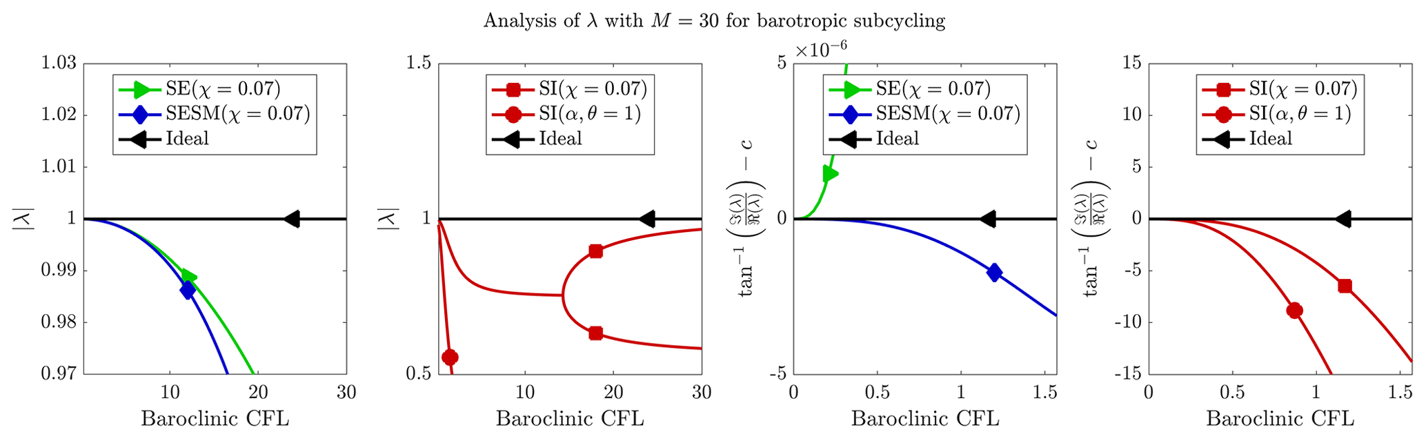
Figure 1Comparison of amplitude and phase error for different schemes using the same dissipation χ=0.07 and maintaining at least second-order accuracy, i.e. , for the SESM scheme as per Eq. (28). Additionally, the SI scheme is also plotted using its recommended configuration , which successfully damps the high phase error solutions corresponding to large CFLs.
This section compares measurements from the new external mode solver to the existing one in FESOM2. The tests are done for both an idealized case and a realistic global setup. The idealized case is expected to highlight threshold performance of the new solver compared to the global case, where its impact will also be governed by mesh non-uniformity, the presence of external forcing, complicated boundaries, and bottom topography. The global case will, however, crucially assess the practicality of this new solver.
4.1 Idealized channel
In Sect. 3 (see Fig. 1), the primary characteristics of the new schemes were explored. In this idealized case, the solvers are tested for correct representation of the mean dynamics. We use the zonally re-entrant channel described in Soufflet et al. (2016). It is 2000 km long (north–south), 500 km wide (east–west), and 4 km deep. We test 10 km meshes of different types (triangular, quadrilateral) and unequally spaced vertical levels (40, 60). The baroclinic time step is τ=720 s, and surface gravity wave speed m s−1 so that a mesh cell is crossed by waves in less than 50 s. We take M=30 for the split-explicit solver, which means s. The initial density stratification due to temperature corresponds to a zonal jet. The zonally mean stratification and velocity are relaxed to their initial distributions. Some initial temperature perturbation leads to an onset of baroclinic instability, which is maintained through the relaxation of the zonal mean profiles. Simulations are run for 20 years, and the last 13 years are used to compute means. Figure 2 shows that mean depth profiles for this case are not affected by implementation of the new solver regardless of mesh configuration, i.e. a different mesh structure and number of vertical layers. This can be attributed to the predominantly baroclinic character of the flow, so the lower dissipation in the new solver is not necessarily seen. This is further supported by the observation that when the bottom drag is reduced, i.e. when the flow is made more barotropic, we see the separation in mean eddy kinetic energy between the two solvers grow, as shown in Fig. A2.
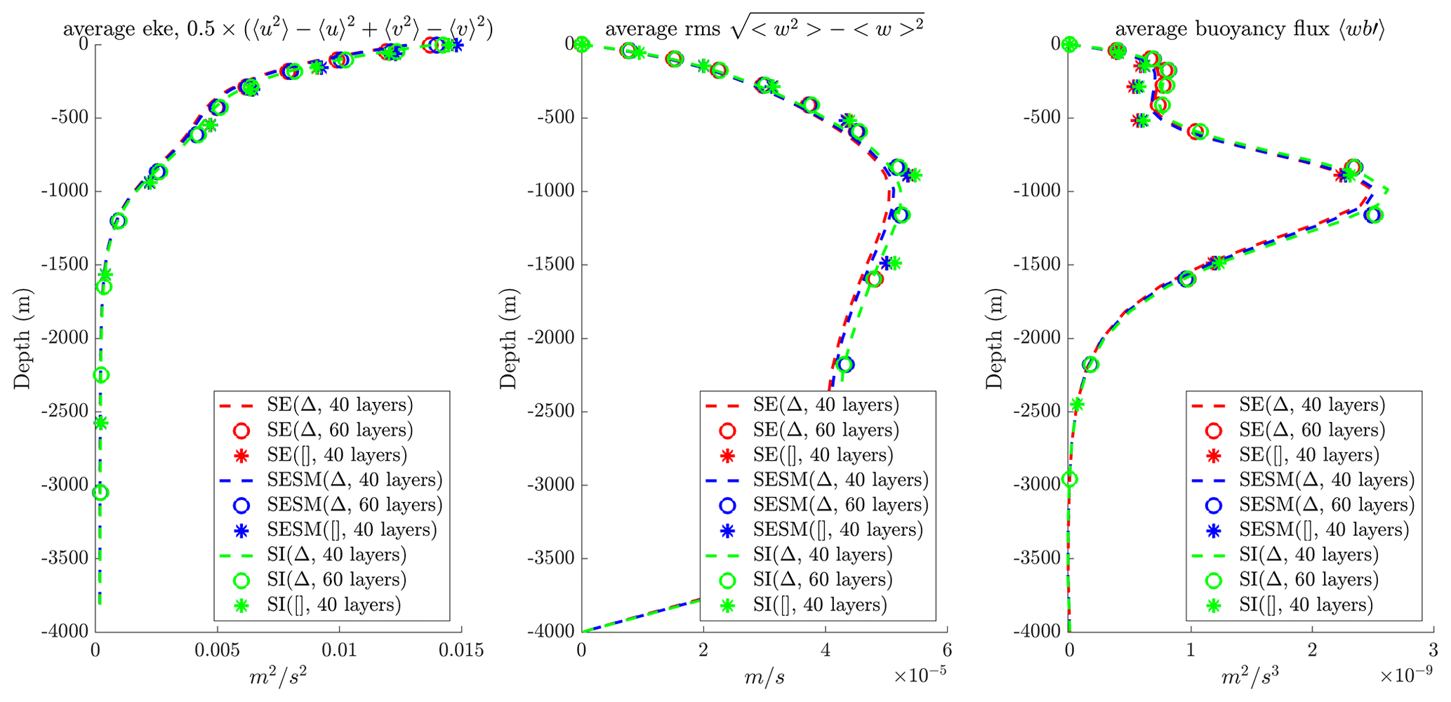
Figure 2Comparison of area-averaged mean depth profiles for eddy kinetic energy (m2 s−2), root-mean-square vertical velocity (m s−1), and buoyancy flux (m2 s−3), with the number of barotropic sub-cycles at M=30. Here, Δ and [] mean triangular and quadrilateral meshes, respectively. The meshes used have a fixed horizontal resolution of 10 km but varying vertical resolutions (40 or 60 layers).
4.2 Surface gravity wave
In this test, we further show how the SE solver for the barotropic mode being proposed is less dissipative and how the differences between it and the current SI solver of FESOM2 become more obvious when the barotropicity of the flow is dominant. For that, we use a simple surface gravity wave (SGW) setup where we simulate a channel (of the same geometry as in Sect. 4.1) with an initial elevation distribution that is meridionally Gaussian, i.e. , where A=3 m is the amplitude and σ=200 km is the half-bell width. The temperature is set at T=20 °C, the velocities are initialized to 0, and the simulation is run for 3 d with a baroclinic time step of τ=5 min. As seen in Fig. 3, which shows the final elevation for both cases after 3 d as well as time series of their available potential energy (APE), the APE for the SI solver asymptotes to 0 within the first 10 h, with the SI solver heavily damping all the SGWs, whereas the SE solver still maintains strong SGWs along with most of its APE. In contrast to the results for the baroclinic test case of Sect. 4.1, here we see a clear difference between the two solvers because of the flow being purely barotropic. As such, we see the gains in terms of the better energetic representation that the new SE solver promises.
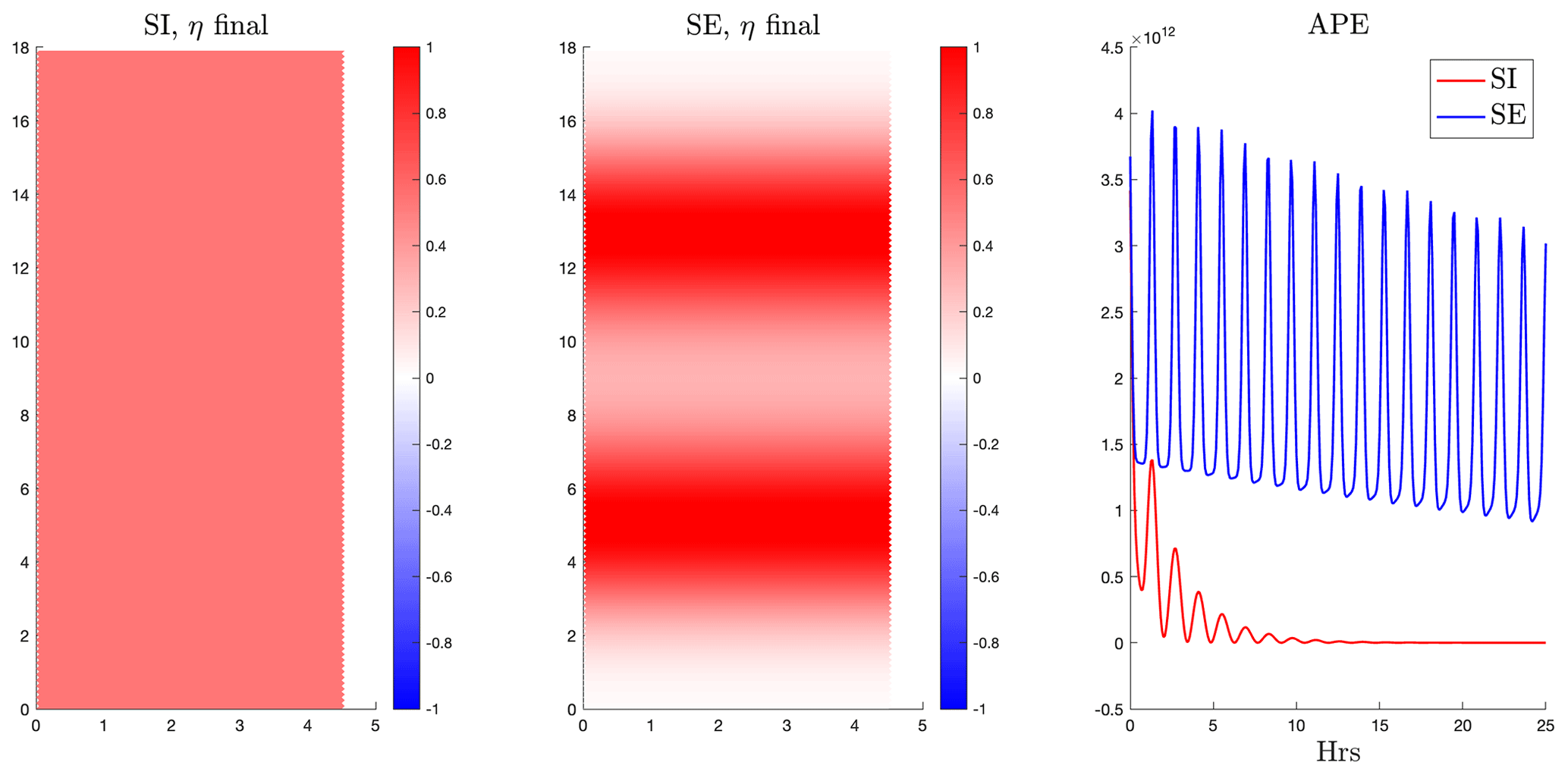
Figure 3Comparison of elevation (m) distribution snapshots for both solvers (after 3 d) and their total available potential energy density (m5 s−2) time series. The number of barotropic sub-cycles are M=30 and θ=0.14 for the SE solver, while for the SI solver, as per the recommended configuration. Here, triangular mesh with sides of 10 km and a baroclinic time step of τ=5 min is used.
4.3 Realistic global ocean
For this case, we now test a more complicated case of a global ocean–sea ice simulation similar to the one used by Scholz et al. (2022). We use the standard coarse mesh of FESOM2 with a minimum resolution of 25 km north of 25° N and a coarse resolution of around 1.5° in the interior of the ocean, with further moderate refinements in the equatorial belt and around Antarctica. The mesh configuration consists of 47 vertical levels with a minimum layer thickness of 10 m near the surface, up to 250 m near the abyssal depth. The baroclinic time step is τ=2700 s, and we take M=50 for the split-explicit solver, which means that s. The simulations were forced with the JRA-55do v1.4.0 reanalysis data covering the period from 1958 to 2019. To show the differences in the simulations carried out with the SI and the SE barotropic solvers, we only show mean elevation, surface temperature, and kinetic energy over the last 20 years (1999–2019) of the simulation period. Due to the high similarity of SE and SESM results (as seen earlier in Fig. 2 for the idealized case), only SE results are shown in Fig. 4. The differences in sea surface elevation are found to be rather small. The pattern of difference in the sea surface temperature is most likely associated with the transient variability that is different in the two setups. The eddy kinetic energy increases everywhere outside the equatorial belt. This increase could be associated with the reduction in overall dissipation due to use of the SE barotropic solver and the observation that the barotropic kinetic energy contributes most to the overall kinetic energy budget at middle and high latitudes, as shown in Aiki et al. (2011).
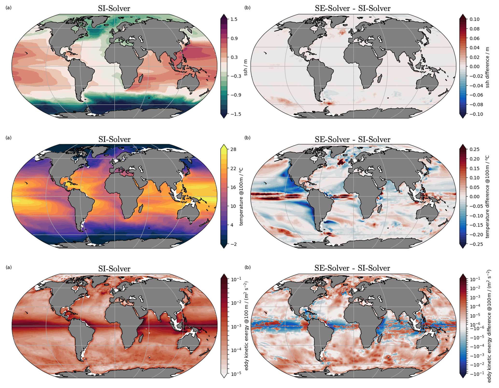
Figure 4Comparison of biases in sea surface heights (m), temperatures (°C), and eddy kinetic energies (m2 s−2) using M=50 barotropic sub-cycles. The SE solver uses dissipation parameter θ=0.14, and depth-dependent fields are at 100 m.
In summary, no significant difference in terms of time-averaged measurements from the new SE external mode solver was observed. For both the idealized and the global test cases, the new SE external mode solver maintained mean dynamics close to those reported by the current SI solver.
This section compares the parallel scalability of the new external mode solver to the existing one of FESOM2. As in Sect. 4, we again utilize the two test cases – idealized and global – described earlier. Additionally, the two cases are also executed on different computer clusters providing for even better estimation of their general performance. Again, because of high similarities between SE and SESM parallel scalability in comparison to SI, the plots of SESM are omitted. In reality, SESM was found to be slightly less scalable than SE. The simulations are run for many model steps, and the mean total time per task the model spends for the barotropic solver is measured. For the idealized case, the simulations were performed using the Ollie HPC at the Alfred Wegener Institute equipped with Intel Xeon E5-2697 v4 (Broadwell) CPUs (308 nodes with 36 cores). To ensure a sufficient workload, we used a fine 2 km triangular mesh with 60 vertical layers on the same channel setup as in Soufflet et al. (2016). The mesh contains approximately 2.5×10⁵ vertices, so the setup is expected to scale almost linearly to about 103 cores, according to our previous experience (Koldunov et al., 2019). The baroclinic time step has been reduced to τ=144 s, and M was left without changes. For this case, the simulations were run for 600 steps, i.e. 1 simulated day. As seen from Fig. 5 (left panel), the new external mode solver (SE) scales significantly better and is faster than the current SI solver of FESOM across all workloads. In reality, the relative speed of the SE versus SI solver will depend on M and on the efficiency of the preconditioner in SI and may change. Since the barotropic solver takes only a part of the total time step (10 %–20 %), the improved scalability of the SE solver contributes noticeably to the reduction in total computing time only after approximately 400 surface vertices per core, as shown in the left panel of Fig. 5. Its impact becomes significant only when parallelized beyond this limit. For the global case, the measurements were performed using the Albedo HPC at the Alfred Wegener Institute with 2xAMD Epyc-7702 CPUs (240 nodes with 128 cores). It uses the same setup and mesh from the global case in Sect. 4. The mesh contains approximately 1.27×10⁵ vertices. The baroclinic time step and M have been left unchanged (τ=2700 s and M=50, respectively). Here, simulations were run for 11 680 steps, i.e. 1 simulated model year. Similar to the findings from the idealized channel case, Fig. 5 (right panel) shows the new SE solver scaling similarly faster and further for the global case also. We again observe a perceivable difference across all workloads. Similar to the idealized case, these performance improvements only become significant for highly parallelized workflows, i.e. for fewer than approximately 400 vertices per core. In summary, the performance of the SE solver shows visible improvement in parallelization and computing time over the SI solver across all tested workloads. The behaviour remained the same over different test cases (idealized and global) and different computer resources (Ollie HPC, Albedo HPC). For less-parallel workloads, the benefits are marginal, but they become significant for highly parallelized workflows, i.e. in cases with fewer than approximately 400 vertices/core.
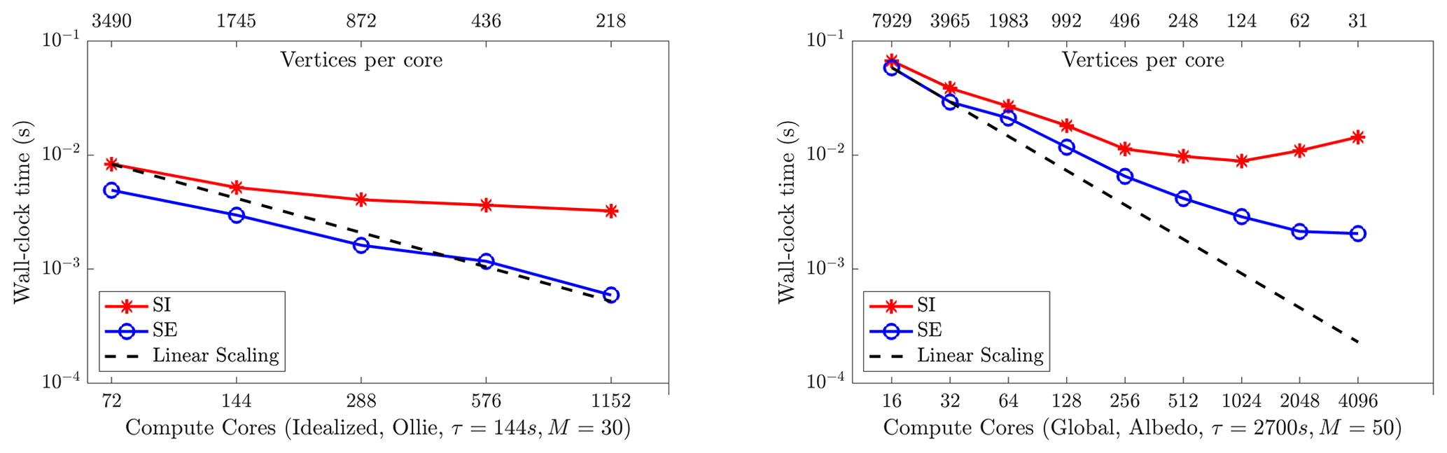
Figure 5Scaling results for the idealized test case with a 2 km uniform mesh on the Ollie HPC cluster and the global test case with a 60–25 km unstructured mesh on the Albedo HPC cluster. The black line indicates linear scaling and the coloured lines give the mean computing time over the parallel partitions for the solver part of the code. Here, the wall-clock time measured corresponds to the model runtime per baroclinic step.
A preliminary implementation of the new split-explicit external mode solver within the sea ice model FESOM2 as proposed in this paper, including the test cases, can be found in the public repository at https://doi.org/10.5281/zenodo.10040944 (Banerjee et al., 2023).
The new split-explicit external mode solver proposed in this paper is more phase accurate, faster, and more scalable than the SI solver used in FESOM (Danilov et al., 2017). The dissipative asynchronous time-stepping scheme (SE) of Demange et al. (2019) is able to deliver phase accuracy orders of magnitude higher than the first-order SI scheme used before. It also provides comparable phase accuracy and dissipation to the dissipatively modified AB3–AM4 scheme (SESM) of Shchepetkin and McWilliams (2005). No filtering of fast dynamics is required due to the dissipative character of the SE solver. It is easier to implement compared to SESM, and leads to very similar results as SESM in practice.
The new SE solver is one part of the adjusted time stepping of FESOM that facilitates the use of the arbitrary Lagrangian–Eulerian vertical coordinate. As a demonstration, we extended z* in FESOM2 to the vertical coordinate in the development version of FESOM2. The implementation of is outlined in Appendix C but still needs to be tested in realistic simulations. Across different test cases using different mesh geometries and computing resources, the new solver is shown to represent mean dynamics similarly to the existing solver with no significant difference. In the case of runtime performance and parallel scalability, it is shown to improve across all workloads. The improvements are shown to be especially significant for highly parallelized workloads. Kang et al. (2021) presents a semi-implicit solver for MPAS, showing that in contrast to the present work, it is more computationally efficient than their split-explicit solver. While a detailed answer to the question why the opposite conclusion was reached needs a separate study, here we can only mention that by following Demange et al. (2019), we perform fewer external time steps per baroclinic time step than in MPAS (Ringler et al., 2013).
We note that on unstructured meshes, a semi-implicit method can be more forgiving than a split-explicit one toward the size of mesh elements. A small element in deep water will hardly affect the solution of the semi-implicit solver but may require an increased number of barotropic substeps in a split-explicit method. This is why the semi-implicit option will be maintained in FESOM alongside the novel split-explicit option. It will however, be modified to allow more general ALE options as described in Appendix B. To conclude, this work suggests that the new split-explicit external mode solver is a good alternative to the existing solver of FESOM2.
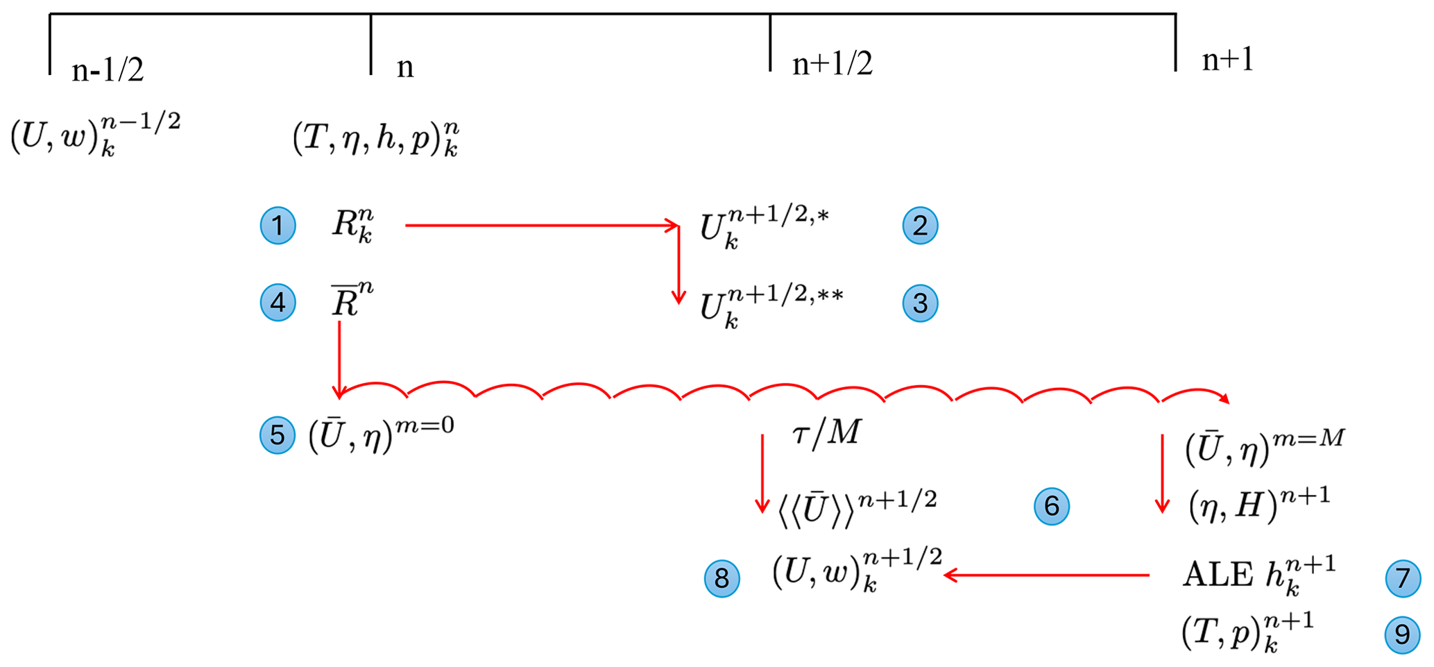
Figure A1Schematic diagram of the control flow for the split-explicit asynchronous time stepping proposed in this paper for FESOM2.
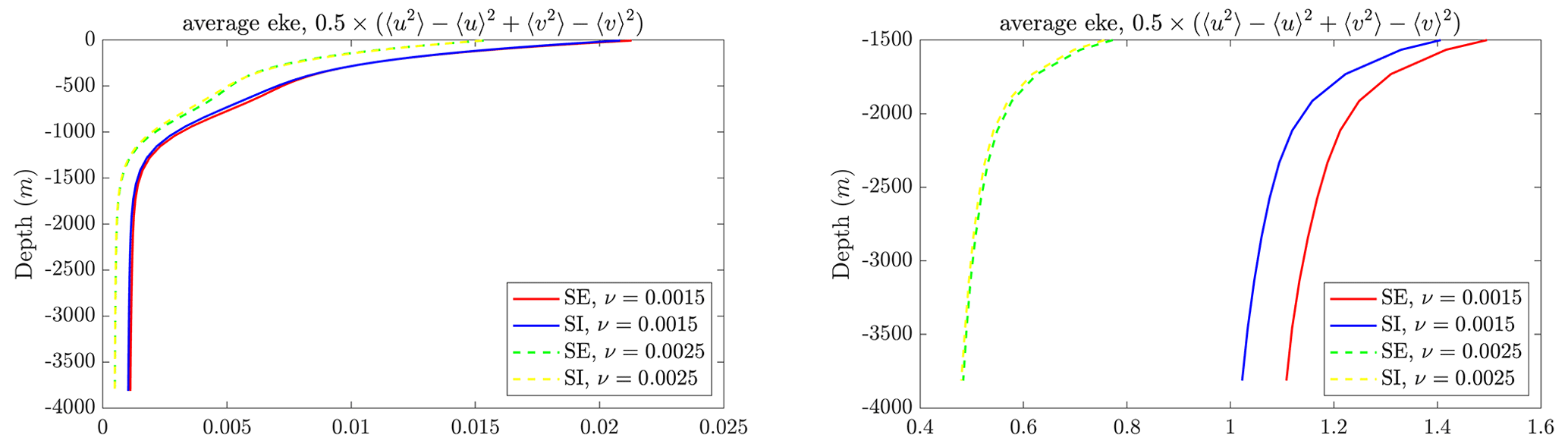
Figure A2Comparison of area-averaged depth profiles for eddy kinetics (m2 s−2) over a period of 10 years simulated with a baroclinic time step of τ=10 min on a 10 km triangular mesh with different linear bottom drags.
The main difference from the split-explicit method is that the elevation η has to be defined at the same time levels as the horizontal velocity. The elevation is therefore detached from the thicknesses, which creates some conceptual difficulty. We consider quantities at and n to be known (to start from velocity).
-
The predictor step is as follows
Here, tilde implies that the contribution from the elevation to the pressure gradient force (PGF) is omitted. It is taken into account explicitly (the last term). However, since is unknown, we take the value from the current time level . Our intention is to get the Semi-Implicit form , in the end. The momentum advection and Coriolis terms are AB2 or AB3 interpolated to n. Implicit vertical viscosity is taken into account by solving
It is solved similarly to the split-explicit asynchronous case.
-
The corrector step is as follows
This step is only written but is evaluated after is available.
-
We write the elevation step as
Here, , which is needed for stability. This equation has to be solved together with the corrector equation. We express from the corrector equation and insert the corrector step into the elevation equation to get
This equation is solved for , giving .
-
The corrector step is used to compute .
-
We write the thickness equation for the ALE step as
These equations are summed vertically to give
The quantity is the elevation at time step n+1. It is used to define hn+1 for the z* vertical coordinate. The extension to follows similarly to the SE case. After hn+1 is defined, w is found from the thickness equation.
-
The tracers are as follows
-
By virtue of the thickness equation above,
We ignore the freshwater flux for simplicity, but it can be added. The solution is
If satisfied initially on cold start by formally taking and , this relationship will persist with time. However, to avoid accumulation of round-off errors, we reset to the right-hand side of the last expression after the computations of . This new will be used only in the next time step. The point here is that the original is computed by an iterative solver, whereby some significant digits are lost. The reset compensates for that. provides centring in time.
Both split-explicit and semi-implicit asynchronous schemes are relatively straightforward to implement. The semi-implicit method with and is non-dissipative, and dissipation is added by shifting θ toward 1. As explained above, even though the dissipation can be controlled well by offsetting only slightly, there are dispersive errors. Since the SI method is used with large Courant numbers for surface gravity waves, the contributions from such waves will come with large phase errors and should be damped. To keep the centring of η, we may take and . FESOM in most applications uses θ=1 and α=1, which implies more dissipation.
In the case of the vertical coordinate (Leclair and Madec, 2011), the horizontal divergence in a layer is split into fast and slow contributions. The fast one modifies layer thickness, and the slow one leads to diasurface w. Examples of practical implementation are provided by Petersen et al. (2015) and Megann et al. (2022). Our implementation presents a simplified version of both. The desired layer thickness is computed as
where corresponds to the z* coordinate, and is the high-frequency component that augments z* to . They will be defined below. The bottom depth in FESOM is a cell-wise constant, whereas elevation and layer thicknesses are defined at vertices. For this reason, for a given vertex v, we modify thicknesses of layers that do not touch topography (see Danilov et al., 2017). The total number of layers under vertex v will be denoted K=K(v). We take
An alternative definition would be to stretch the layers proportionally to their actual thickness, but Megann et al. (2022) warn that some drift in h* may be present in such a case. Excluding the fixed layers, we split the divergence into a quasi-barotropic part that corresponds to and the remaining quasi-baroclinic part (“quasi” because we are limited to K′ layers),
where is the vertically integrated divergence (note that all layers contribute to D). We will be interested in , which is computed as the difference between Dk and . We use the available thicknesses for in Eq. (13) to determine transports featuring in Dk. After is fully specified, we re-trim using defined as a half sum of the thicknesses at full steps. Our treatment of the barotropic part is admittedly less accurate than in Petersen et al. (2015) and Megann et al. (2022), and some barotropic waves will contaminate . However, because of the fixed bottom layers, we have already introduced uncertainty from the very beginning. Since , . The high-frequency thickness will be related to and should sum to zero vertically. D′ is split into low- and high-frequency parts,
The low-frequency part is nudged to as
where τlf is the timescale (about 5 d in Petersen et al., 2015, but larger values can be of interest according to Megann et al., 2022). The fast-frequency part is obtained by subtracting the low-frequency part from . The high-frequency contribution to thickness is
The second term on the right-hand side damps to zero over the timescale τhf (about 30 d). The last term will smooth the thickness, and the diffusivity Khf is determined experimentally. If Khf is vertically constant, if it was initially so. A potential difficulty with Eq. (C2) is that is not bounded. A simple procedure is implemented at present. Equation (C2) is stepped implicitly with respect to the relaxation term, and diffusion is applied in a separate step. If is outside the bounds for any k in the column at vertex v, τhf is adjusted for the entire column at this time step to ensure that will be within the bounds, and computations of are repeated. While this procedure is sufficient for the simple channel test case, it remains to be seen whether it will be sufficient in more realistic cases or whether the solutions reported by Megann et al. (2022) will be needed. The field hhf is always damped stronger at locations close to topography to eliminate possible inconsistencies with hhf=0 in cells touching bottom topography. After is estimated, hn+1 is available; the transports can be re-trimmed, and diasurface velocities can be estimated from the thickness equations.
A preliminary implementation of the new split-explicit external mode solver within the sea ice model FESOM2 as proposed in this paper, including the test cases, can be found in the public repository at https://doi.org/10.5281/zenodo.10040944 (Banerjee et al., 2023).
TB, SD, and KK developed the algorithm. TB, SD, DS, and PS implemented the FESOM prototype and the main FESOM branch. All authors contributed to the writing and discussions.
The contact author has declared that none of the authors has any competing interests.
Publisher’s note: Copernicus Publications remains neutral with regard to jurisdictional claims made in the text, published maps, institutional affiliations, or any other geographical representation in this paper. While Copernicus Publications makes every effort to include appropriate place names, the final responsibility lies with the authors.
This paper is a contribution to the projects M5 (reducing spurious mixing and energetic inconsistencies in realistic ocean modelling applications) and S2 (improved parameterizations and numerics in climate models) of the Collaborative Research Centre TRR 181 “Energy Transfer in Atmosphere and Ocean”.
This research has been supported by the Deutsche Forschungsgemeinschaft (grant no. 274762653).
The article processing charges for this open-access publication were covered by the Alfred-Wegener-Institut Helmholtz-Zentrum für Polar- und Meeresforschung.
This paper was edited by Christopher Horvat and reviewed by Mark R. Petersen and one anonymous referee.
Adcroft, A., Anderson, W., Balaji, V., Blanton, C., Bushuk, M., Dufour, C. O., Dunne, J. P., Griffies, S. M., Hallberg, R., Harrison, M. J., Held, I. M., Jansen, M. F., John, J. G., Krasting, J. P., Langenhorst, A. R., Legg, S., Liang, Z., McHugh, C., Radhakrishnan, A., Reichl, B. G., Rosati, T., Samuels, B. L., Shao, A., Stouffer, R., Winton, M., Wittenberg, A. T., Xiang, B., Zadeh, N., and Zhang, R.: The GFDL global ocean and sea ice model OM4.0: Model description and simulation features, J. Adv. Model. Earth Sy., 11, 3167–3211, https://doi.org/10.1029/2019MS001726, 2019. a
Aiki, H., Richards, K. J., and Sakuma, H.: Maintenance of the mean kinetic energy in the global ocean by the barotropic and baroclinic energy routes: the roles of JEBAR and Ekman dynamics, Ocean Dynam., 61, 675–700, 2011. a
Androsov, A., Fofonova, V., Kuznetsov, I., Danilov, S., Rakowsky, N., Harig, S., Brix, H., and Wiltshire, K. H.: FESOM-C v.2: coastal dynamics on hybrid unstructured meshes, Geosci. Model Dev., 12, 1009–1028, https://doi.org/10.5194/gmd-12-1009-2019, 2019. a
Banerjee, T., Danilov, S., Scholz, P., Klingbeil, K., and Sidorenko, D.: FESOM 2.5 with preliminary Split-Explicit Subcycling (2.5), Zenodo [code and data set], https://doi.org/10.5281/zenodo.10040944, 2023. a, b
Cools, S. and Vanroose, W.: The communication-hiding pipelined BiCGStab method for the parallel solution of large unsymmetric linear systems, Parallel Comput., 65, 1–20, https://doi.org/10.1016/j.parco.2017.04.005, 2017. a
Danilov, S., Sidorenko, D., Wang, Q., and Jung, T.: The Finite-volumE Sea ice–Ocean Model (FESOM2), Geosci. Model Dev., 10, 765–789, https://doi.org/10.5194/gmd-10-765-2017, 2017. a, b, c, d, e, f, g, h, i
Demange, J., Debreu, L., Marchesiello, P., Lemarié, F., Blayo, E., and Eldred, C.: Stability analysis of split-explicit free surface ocean models: implication of the depth-independent barotropic mode approximation, J. Comput. Phys., 398, 108875, https://doi.org/10.1016/j.jcp.2019.108875,, 2019. a, b, c, d, e, f, g, h, i, j, k, l, m
Griffies, S. M., Adcroft, A. J., and Hallberg, R. W.: A primer on the vertical Lagrangian-remap method in ocean models based on finite volume generalized vertical coordinates, J. Adv. Model. Earth Sy., 12, e2019MS001954, https://doi.org/10.1029/2019MS001954, 2020. a
Hallberg, R. and Adcroft, A.: Reconciling estimates of the free surface height in Lagrangian vertical coordinate ocean models with mode-split time stepping, Ocean Model., 29, 15–26, 2009. a
Huang, X., Tang, Q., Tseng, Y., Hu, Y., Baker, A. H., Bryan, F. O., Dennis, J., Fu, H., and Yang, G.: P-CSI v1.0, an accelerated barotropic solver for the high-resolution ocean model component in the Community Earth System Model v2.0, Geosci. Model Dev., 9, 4209–4225, https://doi.org/10.5194/gmd-9-4209-2016, 2016. a, b
Jullien, S., Caillaud, M., Benshila, R., Bordois, L., Cambon, G., Dumas, F., Gentil, S. L., Lemarié, F., Marchesiello, P., Theetten, S., Dufois, F., Le Corre, M., Morvan, G., Le Gac, S., Gula, J., Pianezze, J., and Schreiber, M.: Croco Technical and numerical documentation, Zenodo, https://doi.org/10.5281/zenodo.11036558, 2022. a
Kang, H.-G., Evans, K. J., Petersen, M. R., Jones, P. W., and Bishnu, S.: A Scalable Semi-Implicit Barotropic Mode Solver for the MPAS-Ocean, J. Adv. Model. Earth Sy., 13, e2020MS002238, https://doi.org/10.1029/2020MS002238, 2021. a
Klingbeil, K., Lemarié, F., Debreu, L., and Burchard, H.: The numerics of hydrostatic structured-grid coastal ocean models: state of the art and future perspectives, Ocean Model., 125, 80–105, https://doi.org/10.1016/j.ocemod.2018.01.007, 2018. a
Koldunov, N. V., Aizinger, V., Rakowsky, N., Scholz, P., Sidorenko, D., Danilov, S., and Jung, T.: Scalability and some optimization of the Finite-volumE Sea ice–Ocean Model, Version 2.0 (FESOM2), Geosci. Model Dev., 12, 3991–4012, https://doi.org/10.5194/gmd-12-3991-2019, 2019. a, b
Leclair, M. and Madec, G.: -coordinate, an Arbitrary Lagrangian–Eulerian coordinate separating high and low frequency motions, Ocean Model., 37, 139–152, 2011. a, b
Madec, G., Bourdallé-Badie, R., Chanut, J., Clementi, E., Coward, A., Ethé, C., Iovino, D., Lea, D., Lévy, C., Lovato, T., Martin, N., Masson, S., Mocavero, S., Rousset, C., Storkey, D., Vancoppenolle, M., Müeller, S., Nurser, G., Bell, M., and Samson, G.: NEMO ocean engine, Zenodo [code], https://doi.org/10.5281/zenodo.3878122, 2019. a
Megann, A., Chanut, J., and Storkey, D.: Assessment of the time-filtered Arbitrary Lagrangian-Eulerian coordinate in a global eddy-permitting ocean model, J. Adv. Model. Earth Syst., e2022MS003056, https://doi.org/10.1029/2022MS003056, 2022. a, b, c, d, e, f, g
Petersen, M., Jacobsen, D., Ringler, T., Hecht, M., and Maltrud, M.: Evaluation of the arbitrary Lagrangian–Eulerian vertical coordinate method in the MPAS-Ocean model, Ocean Model., 86, 93–113, 2015. a, b, c, d
Ringler, T., Petersen, M., Higdon, R. L., Jacobsen, D., Jones, P. W., and Maltrud, M.: A multi-resolution approach to global ocean modeling, Ocean Model., 69, 211–232, 2013. a, b
Scholz, P., Sidorenko, D., Danilov, S., Wang, Q., Koldunov, N., Sein, D., and Jung, T.: Assessment of the Finite-VolumE Sea ice–Ocean Model (FESOM2.0) – Part 2: Partial bottom cells, embedded sea ice and vertical mixing library CVMix, Geosci. Model Dev., 15, 335–363, https://doi.org/10.5194/gmd-15-335-2022, 2022. a
Shchepetkin, A. F. and McWilliams, J. C.: A method for computing horizontal pressure- gradient force in an oceanic model with a non-aligned vertical coordinate, J. Geophys. Res., 108, 3090–3124, https://doi.org/10.1029/2001JC001047, 2003. a
Shchepetkin, A. F. and McWilliams, J. C.: The regional oceanic modeling system (ROMS): a split-explicit, free-surface, topography-following-coordinate oceanic model, Ocean Model., 9, 347–404, 2005. a, b, c, d, e, f, g, h, i, j, k, l
Soufflet, Y., Marchesiello, P., Lemarié, F., Jouanno, J., Capet, X., Debreu, L., and Benshila, R.: On effective resolution in ocean models, Ocean Model., 98, 36–50, 2016. a, b
Wang, Q., Danilov, S., Sidorenko, D., Timmermann, R., Wekerle, C., Wang, X., Jung, T., and Schröter, J.: The Finite Element Sea Ice-Ocean Model (FESOM) v.1.4: formulation of an ocean general circulation model, Geosci. Model Dev., 7, 663–693, https://doi.org/10.5194/gmd-7-663-2014, 2014. a
Note that in FESOM, θ is implemented as a tunable parameter. Its value of 0.14 was obtained by Demange et al. (2019) under certain assumptions. However, as is shown in this paper, in practice it has been found to work well.
Note that for the SE case, we integrate transport before elevation η in comparison to this case (SESM). The reason is historical. We follow how these two methods were originally proposed, and in principle, the integrations in SE can be interchanged where the η is integrated first, but the gradient is θ-weighted, similar to the one in SESM. Both, however, should result in identical damping.
Note that alternative formulations of re-trimming are also possible, for example, setting . This is also a valid estimate and was tried, but similar to the case mentioned in the paper, this too was seen to be redundant in practice.
Also note that despite being found to be redundant in practice, the re-trimming was still left in the code.
Here, we are exploring only the physical solution that corresponds to a wave propagating in a negative direction.
- Abstract
- Introduction
- Split-explicit asynchronous time stepping
- Temporal discretization for barotropic solver
- Numerical experiments
- Runtime performance and parallel scalability
- Conclusions
- Appendix A: Supplementary figures
- Appendix B: Adaptation of the semi-implicit scheme in FESOM2
- Appendix C: Implementation of in FESOM2
- Code and data availability
- Author contributions
- Competing interests
- Disclaimer
- Acknowledgements
- Financial support
- Review statement
- References