Design and performance of ELSA v2.0: an isochronal model for ice-sheet layer tracing

We provide a detailed description of the ice-sheet layer age tracer Englacial Layer Simulation Architecture (ELSA) – a model that uses a straightforward method to simulate the englacial stratification of large ice sheets – as an alternative to Eulerian or Lagrangian tracer schemes. ELSA's vertical axis is time, and individual layers of accumulation are modeled explicitly and are isochronal. ELSA is not a standalone ice-sheet model but requires unidirectional coupling to another model providing ice physics and dynamics (the “host model”). Via ELSA's layer tracing, the host model’s output can be evaluated throughout the interior using ice core or radiostratigraphy data. We describe the stability and resolution dependence of this coupled modeling system using simulations of the last glacial cycle of the Greenland ice sheet using one specific host model. Key questions concern ELSA's design to maximize usability, which includes making it computationally efficient enough for ensemble runs, as well as exploring the requirements for offline forcing of ELSA with output from a range of existing ice-sheet models. ELSA is an open source and collaborative project, and this work provides the foundation for a well-documented, flexible, and easily adaptable model code to effectively force ELSA with (any) existing full ice-sheet model via a clear interface.

1 Introduction

Large ice sheets preserve climate–cryosphere interactions of the past, such as accumulation or melt rates, which result in isochronal layers (i.e., layers of same age) with particular characteristics in the ice sheets' interiors. These records are accessible via, e.g., ice cores, which have been used extensively to study the climate of the past and climate–ice interactions (e.g., North Greenland Ice Core Project members, 2004; EPICA Community Members, 2006; Dahl-Jensen et al., 2013). However, ice core data are limited to specific locations and are sparsely available due to their high cost and time consumption. Radar observations, on the other hand, provide three-dimensional englacial stratigraphy data of the Greenland and Antarctic ice sheets (MacGregor et al., 2015; Cavitte et al., 2021). While further data acquisition and processing are required for the Antarctic ice sheet (AntArchitecture, 2017), isochrones have been traced and dated over the majority of the Greenland ice sheet. This high-quality data set, although currently under-exploited, is the ideal tool to evaluate ice-sheet model output with reconstructions based on observations throughout the ice sheet's interior, provided that the model used features an age tracer.

But how can the englacial stratigraphy be modeled accurately? Standard passive tracer tools in glaciology are Eulerian and Lagrangian tracer schemes. However, the Eulerian approach suffers from instability and numerical diffusion effects, while in the Lagrangian approach dispersion of the discrete trace particles causes errors and loss of information with depth (Rybak and Huybrechts, 2003). Semi-Lagrangian schemes – where new particles are spawned at every time step, thereby avoiding some of the drawbacks of regular Lagrangian schemes – have been increasingly used for age tracing with good results (Clarke and Marshall, 2002; Clarke et al., 2005; Lhomme et al., 2005; Goelles et al., 2014). However, semi-Lagrangian schemes require perpetual three-dimensional interpolation to determine the values at the location of newly created particles, which is costly and may deteriorate the solution over time.

More recently, Born (2017) developed an alternative, straightforward approach: an isochronal model where the englacial stratigraphy is modeled explicitly with individual layers of accumulation, driven by surface mass balance. Each layer added is isochronal, i.e., has a fixed timestamp. As time passes and more layers accumulate, ice of older layers flows towards the margin of the ice sheet, and the layers become thinner. This approach faithfully represents the englacial stratification and eliminates unwanted diffusion in the vertical direction as layers never exchange mass. In Born (2017), the isochronal model is a two-dimensional ice-sheet model including ice flow description and parameterization. Born and Robinson (2021) isolated the layer tracer scheme into a separate module and coupled it to the full ice-sheet model Yelmo (described in Robinson et al., 2020), which provides the necessary parameters for the layer tracing. Born and Robinson (2021) then applied this isochronal model to the Greenland ice sheet over the last glacial cycle, demonstrating that it produces a more reliable simulation of the englacial age profile than Eulerian age tracers.

Here we provide the full description of this isochronal model, Englacial Layer Simulation Architecture (ELSA) version 2.0, as an independent tool and with an improved layer accumulation scheme and more parameter choice for flexibility. The workflow of the model and key features are presented in Sect. 2. In Sect. 3, we provide a description and results of the control run with the coupled ELSA–Yelmo setup and the reference radiostratigraphy data set. Section 4 contains the description and results of running ELSA with decreased resolution to decrease its computational requirements, which enables large ensemble runs for ice-sheet model parameter tuning. Section 5 provides a summary and conclusion.

2 Model design and description

ELSA is not a standalone ice-sheet model but requires unidirectional coupling to a full ice-sheet model (the “host model”) providing the boundary conditions related to ice physics (surface mass balance, SMB; basal mass balance, BMB; ice thickness) and ice dynamics (horizontal ice velocities). This setup makes ELSA's layer tracing feature widely applicable, as ultimately any ice-sheet model can be used as the host model.

2.1 Key features

• ELSA explicitly represents individual layers of accumulation, each of which has a fixed timestamp (i.e., each layer is isochronal). Horizontal flow is Eulerian and exclusive to each layer, while vertical change is Lagrangian. Layers never exchange mass; they only become thinner as ice flows towards the margin of the ice sheet and calves or melts. This approach avoids advection across the vertical grid interfaces and eliminates numerical diffusion by design.

• While the vertical grid of ice-sheet models is commonly defined in space, ELSA's vertical grid is defined in time (Born, 2017). The vertical resolution of ELSA is given by how frequently a new layer is added. The isochronal scheme therefore defines depositional age as the grid and layer thickness as an advected property, which is opposite to an Eulerian scheme. Note that layers are not required to be equidistant in time or space.

• ELSA simulates its own layered ice sheet independently of the host model and based entirely on the ice physics and dynamics of the host model. ELSA does not alter the simulation of the host model in any way; it simply adds the feature of tracing the age and thickness of the individual layers comprising the ice sheet. ELSA's ice sheet evolves on the host model's horizontal grid with the same temporal resolution as the host model's.

• It is possible to force ELSA offline by providing input data to ELSA after the host model has completed its simulation. A prerequisite for offline forcing is that the required input data are stored with sufficiently high temporal resolution.

• ELSA's resolution can be controlled with the following parameters: (1) setting the vertical resolution via the parameter layer_resolution for a regular grid or via layer_file for customized isochrones; (2) reducing the horizontal resolution with respect to the host model via the parameter grid_factor; and (3) controlling the coupling period (CP) between the host model and ELSA via the parameter update_factor, i.e., setting ELSA's temporal resolution. Table 1 provides a description of all of ELSA's parameters.

• ELSA is currently available in Fortran 2003, and it is object oriented. Its only dependency is the Library of Iterative Solvers for linear systems (https://www.ssisc.org/lis/, last access: 24 March 2023) (Nishida, 2010), which is used for solving the advection equation.

• ELSA's code is open source and published under the GNU General Public License v3 at https://git.app.uib.no/melt-team-bergen/elsa (last access: 12 September 2024, continuously updated).

Table 1 ELSA's parameters.

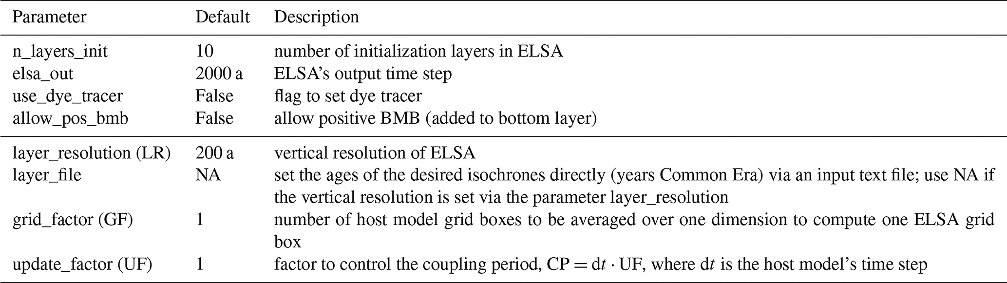
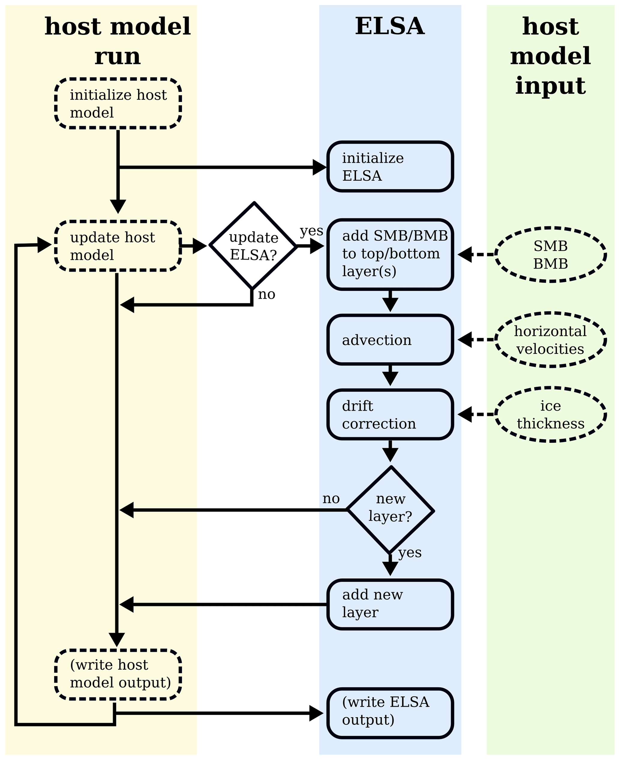
Figure 1 ELSA's workflow and interaction with the host model. The dashed square boxes describe the host model's actions, and the solid square boxes describe ELSA's actions. The dashed oval boxes mark parameters required as input from the host model to ELSA. The diamond-shaped boxes mark decision points in ELSA at temporal and vertical resolutions (see Sect. 2.2.1 for details).

2.2 Design and workflow

The interface between ELSA and the host model is concise and well defined. Over the entire simulation, ELSA requires only surface and basal mass balances, three-dimensional horizontal velocity fields, and ice thickness from the host model. The workflow of the coupled model setup is depicted in Fig. 1 and is executed as follows.

At the beginning of the simulation, ELSA's ice sheet is initialized with 10 equally thick layers (initialization layers). These are typically much thicker than the layers added to the ice sheet during the simulation and do not represent specific isochrones of interest.

After the host model's equilibration and spin-up, the regular model run starts with its defined time step size dt. ELSA can be updated at every time step of the host model (update factor (UF) =1, coupling period (CP) =dt) or less frequently (UF>1, $\text{CP}=\text{UF}\cdot \mathrm{d}t$). Whenever ELSA is updated using the host model's parameters, the following happens:

1. Using the host model's SMB and BMB, the thickness of the top and bottom layers is adjusted. Positive SMB represents snow accumulation and is added to the top layer. Negative SMB represents melt, and the top layer is thinned accordingly. If the top layer is thinner than the amount of melt, its thickness is reduced to zero, and the layer or layers below are thinned accordingly. The host model's BMB is used to adjust the thickness of the bottom layer exclusively (which is an initialization layer). Negative BMB represents melt, and the bottom layer is thinned accordingly. If the host model allows positive BMB, ELSA's flag allow_pos_bmb controls whether the bottom layer can gain thickness.

2. ELSA's individual layers are advected in the horizontal dimension using an Eulerian description of flow (see Appendix B). The passive tracer variable is the layer thickness d, which is advected using an implicit upstream scheme and the host model's horizontal velocities, which are linearly interpolated in the vertical from the original host model's vertical grid of the ice sheet onto the isochronal grid. All layers are advected, where advection is strictly two-dimensional within each isochrone. Therefore, vertical velocities from the host model are not required, and vertical movement in ELSA strictly results from changes in the individual layers' thickness. Layers change thickness due to advection, but they never exchange mass.

3. ELSA's ice-sheet thickness is normalized to the host model ice-sheet thickness to avoid drifting away from the host model state. While this can change layer thickness, the relative thickness of the layers stays constant.

At the end of the ELSA update, a new layer may be added on top of the ice sheet depending on ELSA's vertical resolution, which is either determined by the layer resolution (regular grid) or by manually setting isochrone timestamps. The new top layer is then filled according to the host model's SMB until the next layer is added.

The simulation returns to the host model, where output may be written to file, before the host model proceeds to the next time step to continue the simulation.

In summary, fluxes of mass from the host model are used to dynamically adjust ELSA's top and bottom layer thickness, host model horizontal velocities are used to advect ELSA's layers, and host model ice-sheet thickness is used to normalize ELSA's ice sheet to avoid drifting away from the host model state.

2.2.1 Lowering ELSA's resolution

In the default setup, ELSA solves the advection equation for every layer at every host model grid point and time step, which is computationally costly. Here we describe various ways to decrease the computational cost of ELSA by reducing the spatiotemporal resolution of input data, which is also important for assessing the feasibility of offline simulations. ELSA's spatiotemporal resolution is controlled by the following parameters:

The model parameter layer_resolution (LR) adjusts the vertical resolution in ELSA (how often a new layer is added) for regular vertical grids. A lower vertical resolution means that fewer but thicker layers are advected at every time step. A lower vertical resolution may be acceptable in cases where only a few or selected isochrones are of interest, for example in comparisons with reconstructions. For that, instead of prescribing layer_resolution, the desired isochrones can be set directly with the model parameter layer_file, which is the path to a text file listing all desired isochrone ages.

The model parameter grid_factor (GF) changes the horizontal resolution in ELSA without changing the horizontal resolution of the host model. If set to a value greater than 1, the GF number of host model grid boxes is averaged over both the x direction and the y direction to one ELSA grid box. For example, for GF=3, the average is computed over a total of 9 host model grid boxes to determine 1 ELSA grid box. Values of GF>1 are useful when the horizontal resolution of the host model is much higher than that of, e.g., a data set of reconstructions. Note that GF has to be an integer ≥1.

The model parameter update_factor (UF) controls the coupling period $\text{CP}=\text{UF}\cdot \mathrm{d}t$ between the host model and ELSA, i.e., how often ELSA is updated with the host model's ice parameters. The effect of less frequent coupling is twofold and impacts both accumulated mass balance and advection. The most recent host model SMB and BMB, scaled in time with CP, are used to update the thickness of ELSA's top and bottom layers. In the same manner, the most recent host model horizontal velocities are used to advect all layers in ELSA. While UF>1 decreases run time, it also demonstrates the effect of tracing layers with less information, as would be the case in an offline application of ELSA, fed with less output saved from an ice-sheet model. Note that UF has to be an integer ≥1.

3 Control run setup and results

3.1 Host model setup

We run ELSA online coupled with the open-source thermomechanical ice-sheet model Yelmo. Yelmo solves for the coupled velocity and temperature solutions of the ice sheet (Robinson et al., 2020), where the ice dynamics are solved with a depth-integrated-viscosity approximation (DIVA) approach. Yelmo fully resolves the three-dimensional velocity field, with the three-dimensional shear stress fully represented within the solver. To calculate the three-dimensional field of the effective viscosity, the longitudinal strain rate terms ($\frac{\mathrm{d}u}{\mathrm{d}x}$, $\frac{\mathrm{d}v}{\mathrm{d}y}$) are approximated by the two-dimensional depth-averaged fields, which turns out to be a reasonable approach. A model like Yelmo using the DIVA velocity solver cannot resolve more complex flow like ice folding but can otherwise be expected to represent large-scale continental ice flow with high fidelity.

The model uses Glen's flow law with an exponent of 3. Yelmo can employ an internal adaptive time stepping scheme but is controlled in our experiments by an outer time loop set with a value of dt=10 a. The horizontal grid is an evenly spaced Cartesian grid. We chose to run simulations at a resolution of 16 km as a compromise between speed and output detail for the experiments. The vertical grid is a sigma-coordinate grid (Greve and Blatter, 2009) with 10 layers, which are of higher resolution at the base of the ice sheet. The geothermal heat flux field is prescribed using Shapiro and Ritzwoller (2004). Bedrock and ice topography are taken from Morlighem et al. (2017). The present-day climate is from Fettweis et al. (2017). The past climate is determined transiently using a glacial index method (e.g., Tabone et al., 2018), with the climate interpolated between a present-day and Last Glacial Maximum (LGM) climate field. The LGM climate field is defined as 2 °C colder than the climatological average of several global circulation models from the PMIP3 project (Kageyama et al., 2021), as basal ice temperatures were consistently too warm without the 2 °C adjustment. Surface mass balance is computed using the positive-degree-day (PDD) scheme with a snowmelt factor of 3 $\mathrm{mm}{\mathrm{K}}^{-\mathrm{1}}{\mathrm{d}}^{-\mathrm{1}}$ water equivalent and ice melt factor of 8 $\mathrm{mm}{\mathrm{K}}^{-\mathrm{1}}{\mathrm{d}}^{-\mathrm{1}}$ water equivalent. Basal friction is exponentially scaled with bedrock elevation.

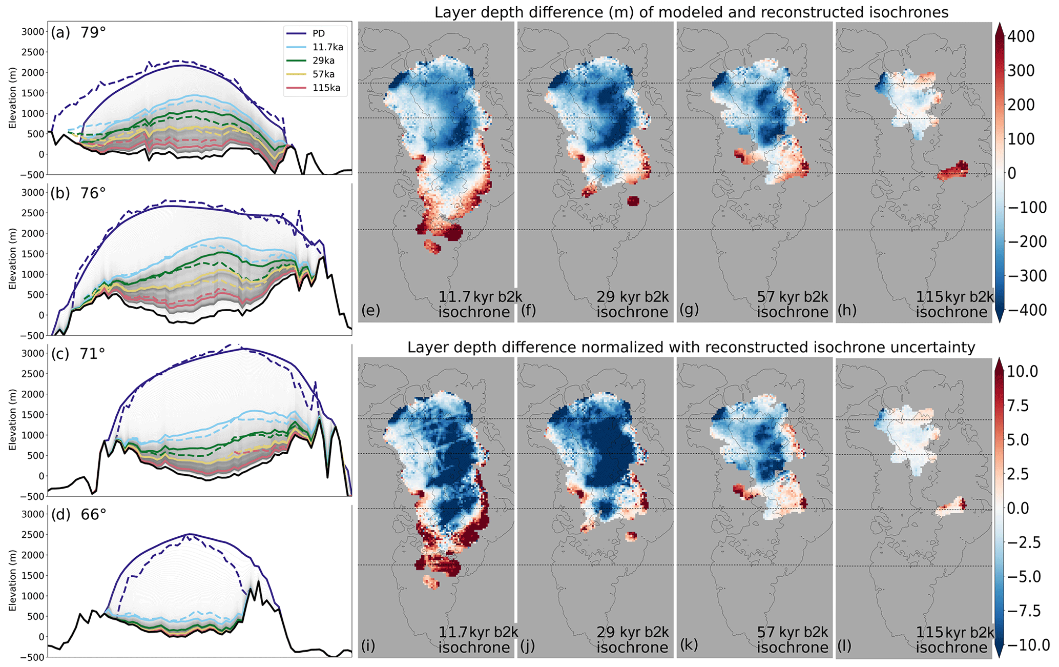
Figure 2 Layer depth differences between modeled and reconstructed isochrones: (a–d) cross sections of the Greenland ice sheet at four different latitudes. The dashed colored lines mark the ice-sheet surface and four isochrones from MacGregor et al. (2015); the equivalent modeled isochrones of the same age are colored accordingly. The thin grey lines mark ELSA's isochrones every 200 a. The thin dotted lines in panels (e)–(l) mark the approximate latitudes of the cross sections. (e–h) Layer depth difference (m) between modeled and reconstructed isochrones. (i–l) Layer depth difference between modeled and reconstructed isochrones, normalized with reconstructed isochrone uncertainty (according to MacGregor et al., 2015).

We used a 700-member ensemble to tune Yelmo parameters and evaluated Eemian ice extent, LGM ice extent, present-day ice extent and thickness, present-day surface velocities, and ice bed properties (frozen versus thawed) to find a suitable Yelmo control (CTRL) run (see Fig. A1). The overall development of the ice-sheet area and volume over the last glacial cycle agrees well enough with previous estimates (e.g., Vasskog et al., 2015), and the present-day bed property state (frozen vs. thawed) is similar to the one assembled by MacGregor et al. (2022).

3.2 ELSA setup

ELSA's parameter UF is set to 1 for this simulation, meaning that advection is updated every 10 years (the same as Yelmo's outer time loop). Simulations are run from 160 kyr BCE until the year 2000 CE (Common Era) with ELSA’s default vertical (layer) resolution of 200 a. Thus the isochronal grid contains a total of 820 layers (10 initialization layers and 810 isochrones) at the end of the simulation. The horizontal grid of the layer tracing scheme is the same as in Yelmo. The ELSA parameter allow_pos_bmb is set to True.

3.3 Isochrone reconstructions

Isochrone reconstructions derived from radiostratigraphy data by MacGregor et al. (2015) can be used to evaluate ELSA's output from the coupled CTRL run. The isochrone dating is based on the Greenland Ice Core Chronology 2005 extended timescale, where age is defined as the year before 2000 CE. For the remainder of the paper, dates and ages with the unit kyr b2k refer to thousands of years before 2000 CE.

MacGregor et al. (2015) provide the depth below the surface and layer depth uncertainty of four dated isochrones of the Greenland ice sheet, as well as ice thickness. The ages of the four reconstructed isochrones are 11.7, 29, 57, and 115 kyr b2k. Isochrone depth uncertainty is a combination of the true depth uncertainty for traced reflections (about 10 m), age uncertainty of the ice core data at the appropriate depth, age uncertainty due to radar range resolution, and uncertainty due to interpolation errors (MacGregor et al., 2015). Layer depth uncertainty for the 11.7 kyr b2k isochrone is mostly below 30 m in the southeast and below 60 m in the northwest of Greenland, for the 29 kyr b2k isochrone mostly below 40 m, for the 57 kyr b2k isochrone mostly below 50 m, and for the 115 kyr b2k isochrone mostly below 100 m (MacGregor et al., 2015).

3.4 Control run results

Comparisons of ELSA's modeled layers with reconstructed ones highlight the areas of isochrone mismatch. In combination with ensemble runs, this evaluation tool provides valuable information to tune the host model's parameters or adjust boundary conditions (e.g., climate forcing) and can be used to find a more realistic representation of ice dynamics and physics in the model simulation.

Cross sections through the present-day ice sheet provide an intuitive way to compare modeled and reconstructed isochrone depth for multiple isochrones at once and demonstrate the value of ELSA's layer tracing. For the Yelmo parameter choice in the CTRL run, these cross sections show that, overall, the isochrones modeled by ELSA match the reconstructed isochrones adequately, where the best agreement is found in the western and central parts of the ice sheet (Fig. 2a–d). In the northeastern part of the ice sheet the three younger modeled isochrones tend to be too high, likely caused by too little precipitation during the Holocene (Ilaria Tabone, personal communication, 2023). Furthermore, the 115 kyr b2k isochrone is consistently too low throughout the entire ice sheet. Note that folding of layers at the base of the ice sheet can present an issue. Layer folding is not modeled by Yelmo or ELSA. Since the reconstructed data we use are processed and quality controlled, we assume that where the 115 kyr b2k isochrone is defined by MacGregor et al. (2015), the presence of folding disturbances has not notably influenced the isochrone's large-scale characteristics. Furthermore, the gridded part of the dated radiostratigraphy data set defines the 115 kyr b2k isochrone only in the north, where accumulation is lower, and the 115 kyr b2k isochrone is thus further away from the base of the ice sheet and closer to the surface. Nevertheless, the specific shortcomings of the 115 kyr b2k isochrone should be kept in mind when using it for model–reconstruction comparison.

As an alternative to cross sections, layer depth differences can be computed for specific isochrones (Fig. 2e–h), which reveals that modeled isochrones tend to be too high in the southern parts of the ice sheet and at the eastern and western margins. Modeled isochrone depths are mostly within 400 m compared to the reconstructed ones and often even within 200 m. While the modeled 115 kyr b2k isochrone is depicted as too low in the panels showing cross sections (Fig. 2a–d), the layer depth difference shows less than 100 m difference (Fig. 2h). This is because modeled isochrone depth is based on the height from the bedrock upwards for the cross sections, while layer depths are computed from the ice-sheet surface downwards, and the different ice thicknesses of the modeled and observed ice sheets are part of the calculation (see also Sect. 3.5).

The difference between modeled and reconstructed isochrone depth normalized with reconstructed layer depth uncertainty provides a third perspective (Fig. 2i–l). Values for normalized isochrone depth difference range from less than −10 to more than 10. A value between −1 and 1 would be ideal, where the modeled and reconstructed isochrone depth difference is less than the uncertainty in the reconstructed isochrones.

Both the parameterization of the ice dynamics and the climatic boundary conditions (mass balance) can be underlying causes of the layer depth difference patterns. The isochrone depth discrepancy in the northeastern part is likely caused by too little precipitation during the Holocene (Ilaria Tabone, personal communication, 2023). Basal friction parameterization, which is still a large source of uncertainty in any ice-sheet model (e.g., Brondex et al., 2019; Choi et al., 2022), influences ice flow throughout the simulation and can therefore contribute to model–reconstruction mismatch in all layers. Note that the comparison with the reconstructed data relies on the ability of Yelmo to simulate the ice sheet well over the last glacial cycle. Our goal in this study is not to evaluate this fit but rather to present the capabilities of ELSA in adding accurate layer tracking to such a model. For the remainder of the study, the above CTRL run can be assumed to be the target for ELSA.

3.5 Limitations

The Library of Iterative Solvers for linear systems, used for solving the advection equation, shows occasional instability where layer thickness can become unrealistically large during one advection step. This error only occurs occasionally and for a few isolated grid cells, often at the ice-sheet boundaries where velocities are large. It is countered by adding a criterion of maximum allowed layer thickness change per advection step (see Appendix B).

Discrepancies between the BedMachine v3 bedrock and true bedrock cause a spiky ice-sheet surface when projecting the ice-sheet thickness from MacGregor et al. (2015) onto the modeled bedrock (Fig. 2b–c, dashed dark blue line particularly on the eastern part). Additionally, the vertical position of the isochrones is affected when visualized from the bedrock upwards, as discussed in Sect. 3.4.

4 ELSA's results for decreased temporal, vertical, and horizontal resolution

We tested numerical strategies in ELSA to decrease run time, and we present how this affects the results. In the following sections, we show the dependence of isochrone depth on the choice of vertical, horizontal, and temporal resolution in ELSA and determine the error introduced compared to the CTRL run described above. To show the horizontal patterns of error magnitudes, we compare layer depths between a simulation with decreased resolution and the CTRL for two specific layers: the 29 kyr b2k isochrone and 115 kyr b2k isochrone. To display the relationship between error magnitude and isochrone age (i.e., depth in the ice sheet), we show the RMSE computed over individual isochrones for every 10 kyr b2k of layer age.

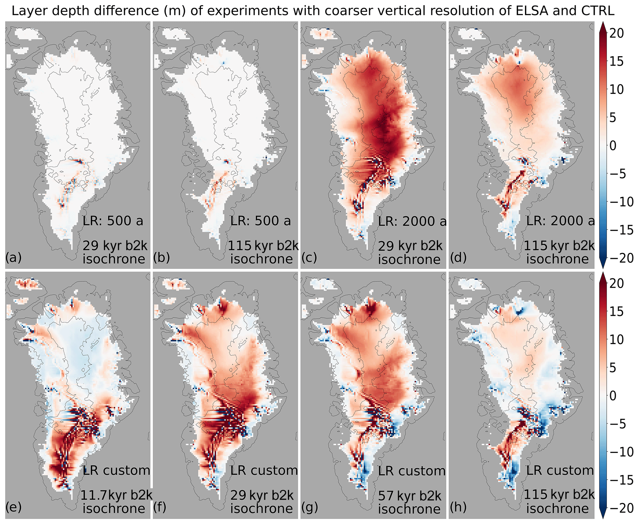
Figure 3 Layer depth difference (m) between model experiments with a coarser ELSA vertical grid and CTRL: LR=500 a for (a) the 29 kyr b2k isochrone and (b) the 115 kyr b2k isochrone; LR=2000 a for (c) the 29 kyr b2k isochrone and (d) the 115 kyr b2k isochrone. The bottom row shows layer depth difference between a simulation with customized isochrone ages and CTRL for the isochrones that match the reconstructed isochrone ages.

4.1 Decreasing the vertical resolution in ELSA

A straightforward way to decrease ELSA's computational cost is by decreasing its vertical resolution; i.e., new layers are added less frequently, and layers are thus thicker. In the CTRL setup, Yelmo runs with 10 vertical levels, which are linearly interpolated in the vertical dimension to provide horizontal velocities for ELSA at the required layers in the ice sheet. ELSA's default vertical resolution is 200 a, which is much finer than the original Yelmo grid for paleo-simulations of several tens of thousands of years.

For decreased vertical resolution in ELSA, layer depth differences are positive over the majority of the ice sheet and generally small: less than 2 m for a layer resolution of 500 a instead of 200 a (Fig. 3a–b) and between 5 and 20 m for a layer resolution of 2000 a instead of 200 a (Fig. 3c–d). These differences occur due to the interpolation of Yelmo velocities onto the finer vertical grid of ELSA and the movement of the isochrones through the vertical velocity profile over the simulation. In the southern part of the ice sheet, where surface mass balance is much larger and deeper layers are consequently much thinner, these interpolation effects show up as dramatic differences in layer depth among neighboring grid cells and downstream effects in the direction of flow. For comparisons with reconstructed data, only the 11.7 kyr b2k isochrone is affected as the older reconstructed layers do not cover the southern area of Greenland.

Instead of setting a fixed vertical resolution and thus a regular vertical grid (in age) for ELSA, the desired isochrone ages, e.g., to match the isochrone ages of the reconstructed data, can be prescribed in a text file, whose path is passed to the parameter layer_file. This is the most effective way to decrease computational cost (see Sect. 4.4). The simulation using only 13 customized isochrone ages (in addition to the 10 initialization layers) shows similar results to the previous experiment: layer depth errors are mostly positive and within 20 m (Fig. 3e–h). The interpolation and downstream effects in the southern part of the ice sheet are more pronounced.

The RMSE computed for several isochrones throughout the ice sheet ranges from less than 0.5 m for LR=400 a to about 4 m for LR=2000 a (Fig. 4). The overall error introduced by decreasing the layer resolution is much smaller than the magnitude of the isochrone depth uncertainty in the reconstructions, and reducing the vertical resolution in ELSA is a good option for decreasing simulation computing time.

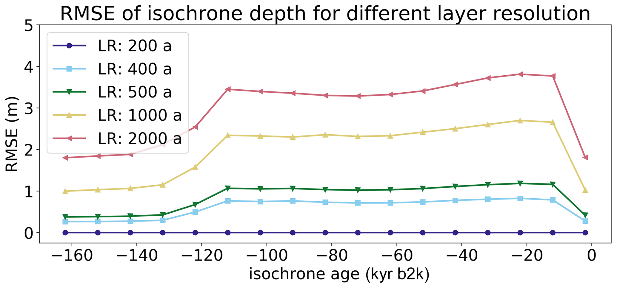
Figure 4 RMSE computed for layer depth difference between model experiments with a coarser vertical ELSA grid and CTRL.

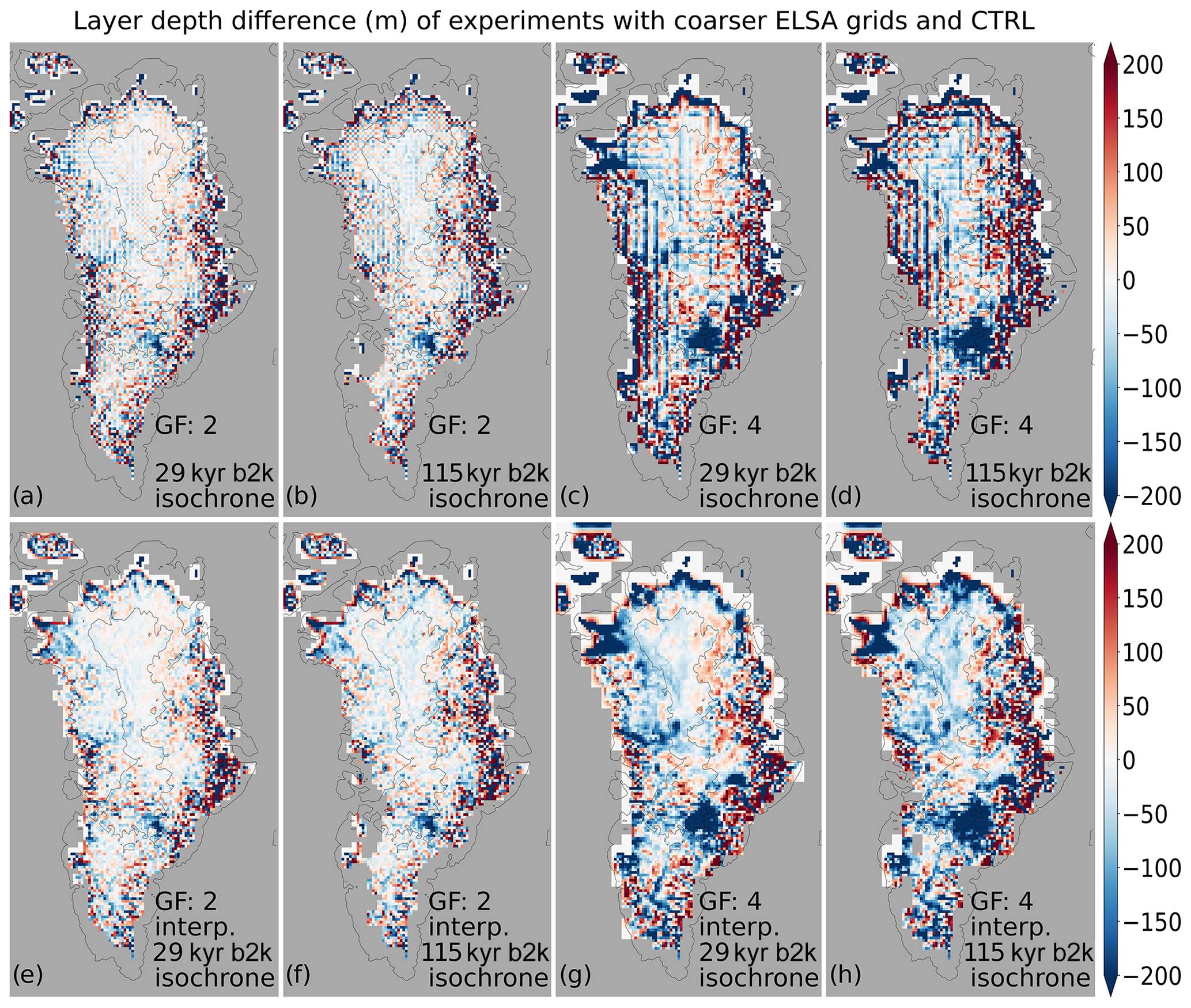
Figure 5 Layer depth difference (m) between model experiments with a coarser ELSA horizontal grid and CTRL: GF=2 for (a) the 29 kyr b2k isochrone and (b) the 115 kyr b2k isochrone; GF=4 for (c) the 29 kyr b2k isochrone and (d) the 115 kyr b2k isochrone. The bottom row shows results for the same settings as the top row but with ELSA output linearly interpolated back to the original grid.

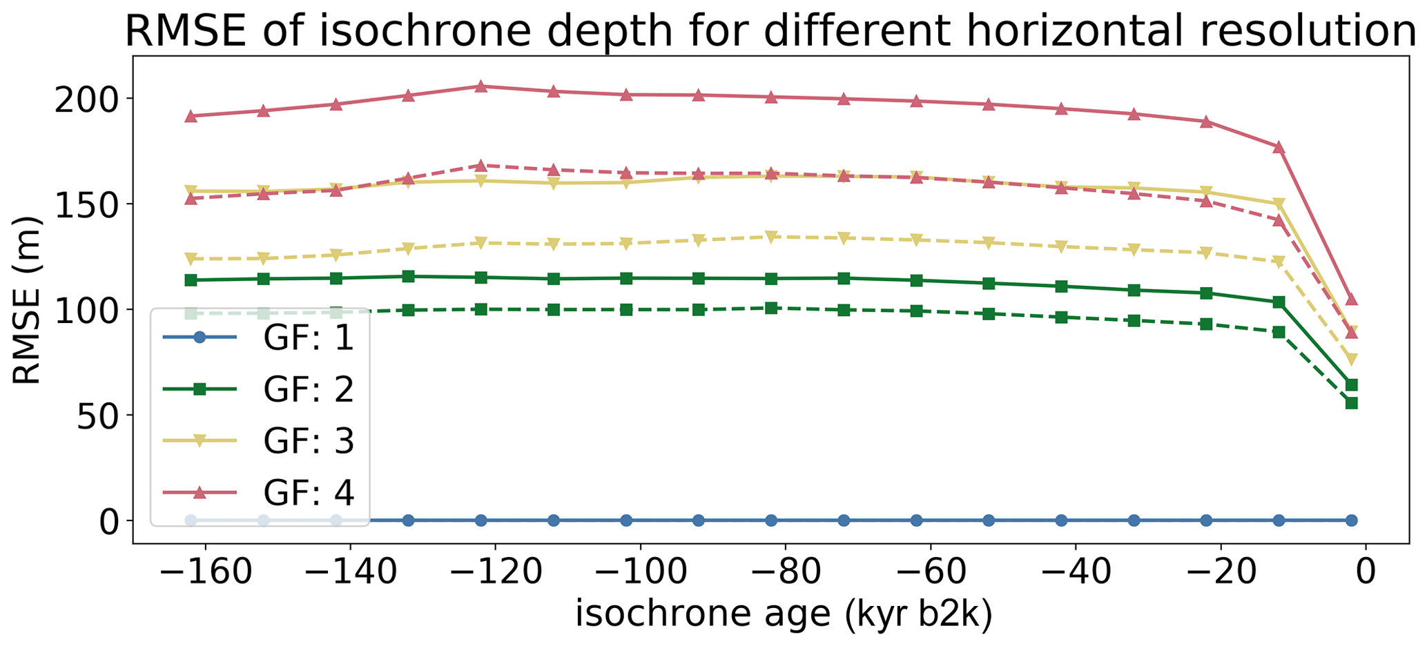
Figure 6 RMSE computed for layer depth difference between model experiments with coarser ELSA horizontal grid and CTRL. The solid lines are the RMSEs on the resulting coarser grid, and dashed lines are the RMSEs for linear interpolation back to the original grid.

4.2 Decreasing the horizontal resolution in ELSA

We decreased the horizontal resolution of ELSA by averaging over an integer number of host model grid cells. We varied GF from 1 (default, 16 km×16 km grid) to 4 (64 km × 64 km grid). As a result, ice thickness and isochrone depth in an ELSA grid box show less horizontal variability compared to ELSA output from the original host model grid (Fig. 5a–d). This effect is much greater at locations with a steeper ice thickness or isochrone depth gradient, i.e., at the ice-sheet margins, with larger values of GF increasing the magnitude of this effect. The overall error pattern does not seem to be related to mass balance or dynamics of the ice sheets.

In the ice-sheet center, the errors range from −50 to 40 m for GF=2 (Fig. 5a–b) and from −120 to 50 m for GF=4 (Fig. 5c–d). At the margins, the errors reach values of more than 500 m. Linearly interpolating the final results from the coarser grid back to the original grid particularly smooths the error in the center of the ice sheet and reduces them to the values around 30 m (Fig. 5e–h). The errors at the margins are mostly unaffected by the interpolation and remain large.

In summary, the overall error introduced by increasing GF is about 0.5–3 times the magnitude of the reconstructed isochrone depth uncertainty, depending on the location. The larger errors at the margins for increased GF are not that relevant to isochrone applications as the radiostratigraphy data are only available for the ice-sheet center, and the issues at the margins do not propagate backwards to the ice-sheet center.

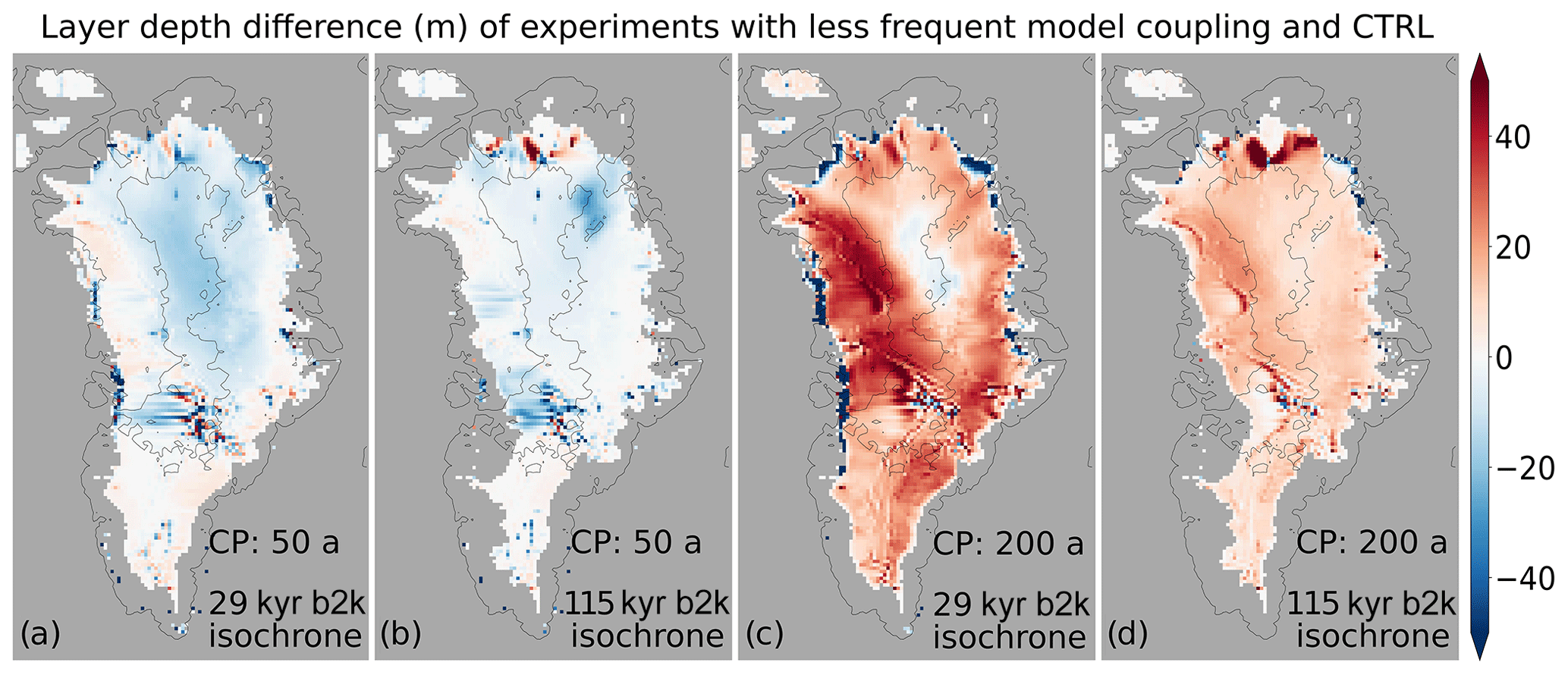
Figure 7 Layer depth difference (m) between model experiments with less frequent coupling of ELSA and Yelmo: CP=50 a for (a) the 29 kyr b2k isochrone and (b) the 115 kyr b2k isochrone; CP=200 a for (c) the 29 kyr b2k isochrone and (d) the 115 kyr b2k isochrone.

The RMSE computed for several isochrones throughout the ice sheet ranges from about 120 m for GF=2 to 200 m for GF=4 (Fig. 6, solid lines). These large RMSEs are strongly influenced by large differences at the ice-sheet margins between the GF experiments and CTRL. Over isochrone age, the RMSE stays mostly constant. The exceptions are the youngest few layers, where the RMSE reduces by about 25 % due to smaller differences at the ice-sheet margins, particularly in the northeast (not shown).

Interpolation to the original grid reduces the RMSE to about 100 m for GF=2 and about 160 m for GF=4 (Fig. 6, dashed lines). Since the interpolation mainly smooths differences in the ice-sheet center but does not significantly improve the results at the margins, the RMSE remains high overall.

4.3 Decreasing the temporal resolution of ELSA

The temporal resolution of ELSA can be reduced by increasing the coupling period (CP) between the host model and ELSA, as would also be the case in an offline application of ELSA using saved host model output. We varied CP from 10 a (default) to 200 a (UF from 1 to 20).

Layer depth differences for a coupling period of 50 a range from −25 to 5 m (Fig. 7a–b), while differences for a coupling period of 200 a are primarily positive and mostly range from 5 to 45 m (Fig. 7c–d). These errors are smaller than or comparable to reconstructed isochrone depth uncertainty.

The RMSE computed for several isochrones throughout the ice sheet depicts the instability of varying coupling periods: for values of CP except for CP=40 a, the RMSE is below 40 m and is close to constant with isochrone age. For CP=40 a, however, the RMSE increases up to 80 m, and the two-dimensional layer depth difference over specific isochrones is very irregular (not shown).

This model instability is relevant when using ELSA offline and forcing it with ice-sheet model output if the temporal resolution of the saved host model output is not sufficiently high. Further investigation of offline setup with specific host models is recommended.

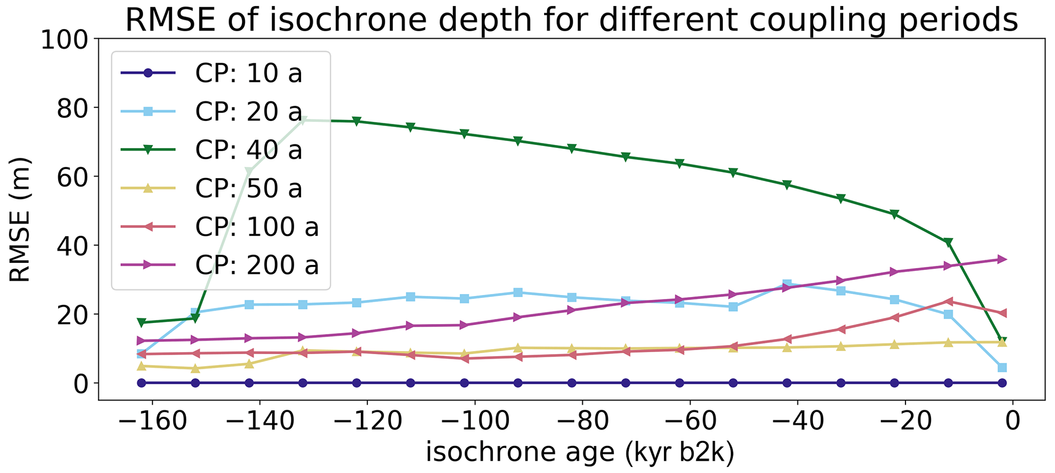
Figure 8 RMSE computed for layer depth difference between model experiments with longer coupling periods between ELSA and Yelmo compared to CTRL.

4.4 Resolution and model speed

With the right setup, it is computationally quite cheap to add ELSA to an ice-sheet model run, with the added benefit of enabling the evaluation of the run using ELSA's output and reconstructed isochrone data. Computational cost is evaluated through model run speed (kiloyear simulation time per computational hour) on a compute node using Intel Xeon Gold 6136 CPUs. The run speed of Yelmo itself is 20.8 kyr h⁻¹ (Fig. 9, dashed black line) in our single thread setup. When customized to only 13 specific isochrones, the coupled ELSA–Yelmo model setup runs with 18.9 kyr h⁻¹, almost as fast as the Yelmo standalone speed. Run speed drops to 4.4 kyr h⁻¹ for the coupled ELSA–Yelmo setup with the CTRL parameter settings (dark blue bars). Decreasing the vertical, horizontal, and temporal resolutions increases run speed, but gain in run speed is not linearly proportional to the decrease in resolution; instead, it is logarithmic. Furthermore, a decrease in horizontal and temporal resolutions introduces errors.

Picking a few specific isochrones of interest is therefore by far the fastest and most accurate coupled model run. Adding isochrones on a regular vertical grid may be necessary for runs on shorter timescales to investigate flow patterns within the ice sheet. Reduced temporal resolution is most likely necessary when using ELSA offline and when host model output is not available at every model time step.

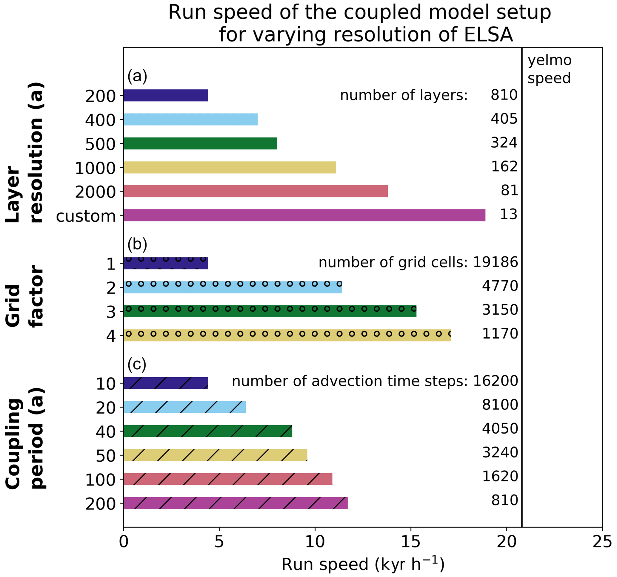
Figure 9 Run speed (kyr h⁻¹) for different parameterizations of ELSA's vertical (a), horizontal (b), and temporal (c) resolutions, as used in the experiments in Sect. 4. The solid black line shows run speed for the Yelmo standalone run. The greatest increase in run speed is achieved when choosing a few specific isochrones of interest. Initialization layers are not included in the number of layers noted in the figure.

5 Conclusions

We described the workflow and features of Englacial Layer Simulation Architecture (ELSA), an isochronal model that can be coupled to a full ice-sheet model (host model) for layer age tracing in an ice sheet's interior. ELSA models individual layers of accumulation explicitly, driven by surface mass balance. Each layer added is isochronal, i.e., has a fixed timestamp. As time passes and more layers accumulate, the ice of older layers flows towards the margin of the ice sheet, and the layers become thinner. This straightforward approach to modeling the englacial stratigraphy avoids issues present in alternative layer age tracers, such as numerical diffusion.

ELSA's computational cost can be decreased by reducing its vertical, horizontal, or temporal resolution. The fastest and preferred way is specifying a number of isochrones instead of a regular vertical grid, which not only increases run speed, but also introduces only a very small error. Decreasing the horizontal resolution of ELSA with respect to the host model also leads to an increase in run speed but introduces errors of the order of tens to hundreds of meters, depending on the degree of resolution depreciation and location. Decreasing the temporal resolution of ELSA with respect to the host model (i.e., less frequent coupling) introduces an error magnitude comparable to reconstructed isochrone depth uncertainty; however, the model runs are not stable in all configurations.

To our knowledge, this is currently the only isochronal model for ice sheets and will thus be a valuable comparison tool with Eulerian, Lagrangian, and semi-Lagrangian layer tracers. Applicability also includes the usage of ELSA for a host model's parameter tuning via ensemble runs (Born and Robinson, 2021). Lastly, this work is the foundation for an offline application of ELSA, further increasing opportunities to evaluate any given ice-sheet model based on its englacial stratigraphy.

Appendix A: Control run results

Figure A1 shows the Yelmo results of the CTRL run (described in Sect. 3): ice thickness and extent at the end of the simulation (year 2000 CE), ice thickness and extent during the Last Glacial Maximum, ice thickness and extent during the Eemian, the difference in present-day ice thickness with respect to BedMachine v3, the difference in present-day ice surface velocity with respect to Joughin et al. (2018), and bed properties at the end of the simulation.

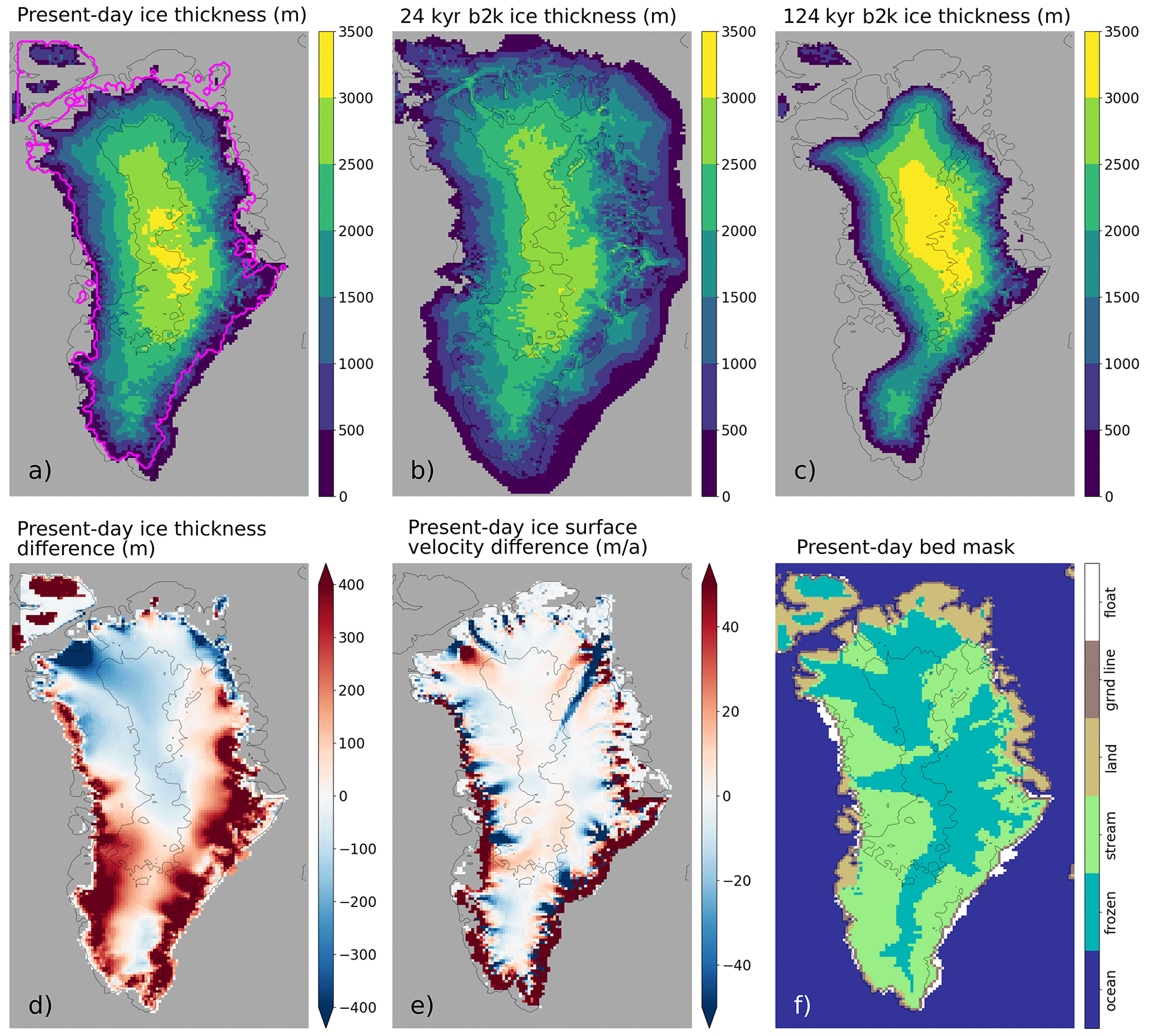
Figure A1 Model CTRL run results: (a) present-day ice thickness (the pink line marks the BedMachine v3 outline, Morlighem et al., 2017), (b) ice thickness and extent during the Last Glacial Maximum, (c) ice thickness and extent during the Eemian, (d) present-day ice thickness difference compared to BedMachine v3, (e) present-day velocity difference compared to Joughin et al. (2018), (f) present-day bed properties.

Appendix B: Layer advection

ELSA uses a Lagrangian description of flow in the vertical dimension but the computationally cheaper Eulerian description of flow in the horizontal dimension within the individual layers. With this approach, numerical diffusion is eliminated by design in the vertical as layers never exchange mass. In the horizontal, numerical diffusion does affect the flow as it uses a finite-difference scheme. However, numerical diffusion comes about in the presence of steep gradients, and natural tracers in ice sheets generally vary smoothly in the horizontal (see also Born, 2017).

The change in the layer thickness d in the x and y directions over time t is given by the divergence of the flow of volume F:

$$\begin{array}{}\text{(B1)}& \begin{array}{rl}{\displaystyle \frac{\partial d}{\partial t}}& =-\mathrm{\nabla }\cdot \mathbf{F}=-({\displaystyle \frac{\partial }{\partial x}},{\displaystyle \frac{\partial }{\partial y}})\cdot \mathbf{F}(x,y)\\ & =-{\displaystyle \frac{\partial }{\partial x}}ud-{\displaystyle \frac{\partial }{\partial y}}vd,\end{array}\end{array}$$

where u and v are the horizontal ice velocities in the x and y directions, respectively.

Equation (B1) is discretized forward in time and upstream in space to

$$\begin{array}{}\text{(B2)}& \begin{array}{rl}{\displaystyle \frac{d_{i,j}^{t+\mathrm{1}}-d_{i,j}^t}{\mathrm{\Delta }t}}& =-u_{i-\mathrm{1}/\mathrm{2},j}^t\cdot {\displaystyle \frac{d_{i,j}^{t+\mathrm{1}}-d_{i-\mathrm{1},j}^{t+\mathrm{1}}}{\mathrm{\Delta }x}}\\ & -d_{i,j}^{t+\mathrm{1}}\cdot {\displaystyle \frac{u_{i+\mathrm{1}/\mathrm{2},j}^t-u_{i-\mathrm{1}/\mathrm{2},j}^t}{\mathrm{\Delta }x}}\\ & -v_{i,j-\mathrm{1}/\mathrm{2}}^t\cdot {\displaystyle \frac{d_{i,j}^{t+\mathrm{1}}-d_{i,j-\mathrm{1}}^{t+\mathrm{1}}}{\mathrm{\Delta }y}}\\ & -d_{i,j}^{t+\mathrm{1}}\cdot {\displaystyle \frac{v_{i,j+\mathrm{1}/\mathrm{2}}^t-v_{i,j-\mathrm{1}/\mathrm{2}}^t}{\mathrm{\Delta }y}}\end{array}\end{array}$$

for positive values of u and v and

$$\begin{array}{}\text{(B3)}& \begin{array}{rl}{\displaystyle \frac{d_{i,j}^{t+\mathrm{1}}-d_{i,j}^t}{\mathrm{\Delta }t}}& =-u_{i+\mathrm{1}/\mathrm{2},j}^t\cdot {\displaystyle \frac{d_{i+\mathrm{1},j}^{t+\mathrm{1}}-d_{i,j}^{t+\mathrm{1}}}{\mathrm{\Delta }x}}\\ & -d_{i,j}^{t+\mathrm{1}}\cdot {\displaystyle \frac{u_{i+\mathrm{1}/\mathrm{2},j}^t-u_{i-\mathrm{1}/\mathrm{2},j}^t}{\mathrm{\Delta }x}}\\ & -v_{i,j+\mathrm{1}/\mathrm{2}}^t\cdot {\displaystyle \frac{d_{i,j+\mathrm{1}}^{t+\mathrm{1}}-d_{i,j}^{t+\mathrm{1}}}{\mathrm{\Delta }y}}\\ & -d_{i,j}^{t+\mathrm{1}}\cdot {\displaystyle \frac{v_{i,j+\mathrm{1}/\mathrm{2}}^t-v_{i,j-\mathrm{1}/\mathrm{2}}^t}{\mathrm{\Delta }y}}\end{array}\end{array}$$

for negative values of u and v. Velocities are used at the faces of the grid cells.

We solve implicitly for d^t+1 with

$$\begin{array}{}\text{(B4)}& {\mathit{d}}^{\mathit{t}}=\mathbf{\text{A}}{\mathit{d}}^{\mathit{t}\mathbf{+}\mathbf{1}},\end{array}$$

where the main and secondary diagonals of A are filled using Eqs. (B2) and (B3) and are given as

$$\begin{array}{}\text{(B5)}& {\displaystyle }\begin{array}{rl}{d}_{i,j}^t& =d_{i,j}^{t+\mathrm{1}}(\mathrm{1}+{\displaystyle \frac{\mathrm{\Delta }t}{\mathrm{\Delta }x}}{u}_{i+\mathrm{1}/\mathrm{2},j}^t+{\displaystyle \frac{\mathrm{\Delta }t}{\mathrm{\Delta }y}}{v}_{i+\mathrm{1}/\mathrm{2},j}^t)\\ & -d_{i-\mathrm{1},j}^{t+\mathrm{1}}{\displaystyle \frac{\mathrm{\Delta }t}{\mathrm{\Delta }x}}{u}_{i-\mathrm{1}/\mathrm{2},j}^t-d_{i,j-\mathrm{1}}^{t+\mathrm{1}}{\displaystyle \frac{\mathrm{\Delta }t}{\mathrm{\Delta }y}}{v}_{i-\mathrm{1}/\mathrm{2},j}^t\\ \text{for }& u_{i,j}>\mathrm{0.1},v_{i,j}>\mathrm{0.1},\end{array}\text{(B6)}& {\displaystyle }\begin{array}{rl}{d}_{i,j}^t& =d_{i,j}^{t+\mathrm{1}}(\mathrm{1}-{\displaystyle \frac{\mathrm{\Delta }t}{\mathrm{\Delta }x}}{u}_{i-\mathrm{1}/\mathrm{2},j}^t-{\displaystyle \frac{\mathrm{\Delta }t}{\mathrm{\Delta }y}}{v}_{i-\mathrm{1}/\mathrm{2},j}^t)\\ & +d_{i+\mathrm{1},j}^{t+\mathrm{1}}{\displaystyle \frac{\mathrm{\Delta }t}{\mathrm{\Delta }x}}{u}_{i+\mathrm{1}/\mathrm{2},j}^t+d_{i,j+\mathrm{1}}^{t+\mathrm{1}}{\displaystyle \frac{\mathrm{\Delta }t}{\mathrm{\Delta }y}}{v}_{i+\mathrm{1}/\mathrm{2},j}^t\\ \text{for }& u_{i,j}<-\mathrm{0.1},v_{i,j}<-\mathrm{0.1},\end{array}\text{(B7)}& {\displaystyle }\begin{array}{rl}{d}_{i,j}^t& =d_{i,j}^{t+\mathrm{1}}(\mathrm{1}+{\displaystyle \frac{\mathrm{\Delta }t}{\mathrm{\Delta }x}}{u}_{i+\mathrm{1}/\mathrm{2},j}^t-{\displaystyle \frac{\mathrm{\Delta }t}{\mathrm{\Delta }y}}{v}_{i-\mathrm{1}/\mathrm{2},j}^t)\\ & -d_{i-\mathrm{1},j}^{t+\mathrm{1}}{\displaystyle \frac{\mathrm{\Delta }t}{\mathrm{\Delta }x}}{u}_{i-\mathrm{1}/\mathrm{2},j}^t+d_{i,j+\mathrm{1}}^{t+\mathrm{1}}{\displaystyle \frac{\mathrm{\Delta }t}{\mathrm{\Delta }y}}{v}_{i+\mathrm{1}/\mathrm{2},j}^t\\ \text{for }& u_{i,j}>\mathrm{0.1},v_{i,j}<-\mathrm{0.1},\end{array}\text{(B8)}& {\displaystyle }\begin{array}{rl}{d}_{i,j}^t& =d_{i,j}^{t+\mathrm{1}}(\mathrm{1}-{\displaystyle \frac{\mathrm{\Delta }t}{\mathrm{\Delta }x}}{u}_{i-\mathrm{1}/\mathrm{2},j}^t+{\displaystyle \frac{\mathrm{\Delta }t}{\mathrm{\Delta }y}}{v}_{i+\mathrm{1}/\mathrm{2},j}^t)\\ & +d_{i+\mathrm{1},j}^{t+\mathrm{1}}{\displaystyle \frac{\mathrm{\Delta }t}{\mathrm{\Delta }x}}{u}_{i+\mathrm{1}/\mathrm{2},j}^t-d_{i,j+\mathrm{1}}^{t+\mathrm{1}}{\displaystyle \frac{\mathrm{\Delta }t}{\mathrm{\Delta }y}}{v}_{i-\mathrm{1}/\mathrm{2},j}^t\\ \text{for }& u_{i,j}<-\mathrm{0.1},v_{i,j}>\mathrm{0.1}.\end{array}\end{array}$$

At the domain boundaries as well as for $-\mathrm{0.1}<u<\mathrm{0.1}$ and $-\mathrm{0.1}<v<\mathrm{0.1}$ m a⁻¹, layer thickness is unchanged.

The Library of Iterative Solvers for linear systems shows occasional instabilities where layer thickness becomes unrealistically large during one advection step. We introduced a maximum allowed layer thickness change per advection step, d_diff (m), which is defined as

$$\begin{array}{}\text{(B9)}& d_{\text{max}}=\mathrm{100}+\mathrm{10}\text{update\_factor}+\text{layer\_resolution}/\mathrm{10}.\end{array}$$

For the default settings of update_factor = 1 and layer_resolution = 200, d_diff=130 m.