Prediction of hysteretic matric potential dynamics using artificial intelligence: application of autoencoder neural networks

Information on soil water potential is essential to assessing the soil moisture state, to prevent soil compaction in weak soils, and to optimize crop management. When there is a lack of direct measurements, the soil water potential values must be deduced from soil water content dynamics that can be monitored at the plot scale or obtained at a larger scale from remote sensing information. Because the relationship between water content and soil water potential in natural field soils is highly ambiguous, the prediction of soil water potential from water content data is a big challenge. The hysteretic relationship observed in nine soil profiles in the region of Solothurn (Switzerland) is not a simple function of texture or wetting–drainage cycles but depends on seasonal patterns that may be related to soil structural dynamics. Because the physical mechanisms governing seasonal hysteresis are unclear, we developed a deep neural network model that predicts water potential changes using rainfall, potential evapotranspiration, and water content time series as inputs. To adapt the model for multiple locations, we incorporated a deep autoencoder neural network as a classifier. The autoencoder compresses the water content time series into a site-specific feature that is highly representative of the underlying water content dynamics of each site and quantifies the similarity of dynamic patterns. By adding the autoencoder's output as an additional input and training the neural network model with three stations located in three major classes established by the autoencoder, we predict matric potential for other sites. This method has the potential to deduce the dynamics of matric potential from water content data (including satellite data) despite strong seasonal effects that cannot be captured by standard methods.

1 Introduction

The soil water characteristic curve (SWCC) relates the matric potential (MP) and water content (WC) and is the key physical property in quantifying soil water dynamics (Tuller and Or, 2023). The SWCC (also termed the soil water retention curve or pressure–saturation relationship) depends on both soil texture and soil structure and differs according to soil type and soil textural class (Rawls et al., 2003; Shwetha and Varija, 2015). The SWCC contains information on the pore size distribution and allows the assessment of flow and transport properties for different hydration states (Menon et al., 2020; Rostami et al., 2015). To provide a complete characterization of the actual soil moisture state and flow regimes, information on both the matric potential and the water content must be specified. Information on volumetric water content is needed to assess the free storage capacity, optimize water management, and formulate mass balance. The matric water potential is a component of the total and hydraulic soil water potential and determines the water flow in the direction of decreasing water potential to achieve equilibrium with its surroundings (Ma et al., 2022). The matric potential is also of particular interest in assessing the mechanical stability of a soil (Holthusen et al., 2010; Lu et al., 2010). The capillary and adsorptive forces expressed with the matric potential define the unsaturated soil strength mitigating soil compaction by heavy machinery in construction work, farming, and forestry (Smith et al., 2001). For example, matric potential thresholds are defined in various regions of Switzerland to prevent mechanical damage and regulate the maximum load linked to factors like soil type, texture, and vehicle impact (Bundesamt für Energiewirtschaft, 1997). Other important potential thresholds are the wilting point and the field capacity, which characterize the plant-available water (Gupta et al., 2023).

It would be optimal to determine the soil moisture status relative to these potential thresholds based on information of water content using the SWCC, without direct measurement of the matric potential. In that case, matric potential dynamics could be deduced from remote sensing water content data that are available at various scales. However, the application of this procedure is limited by two effects. Firstly, under saturated conditions, the water potential can change without modifying the volumetric water content. The transition of conditions with negative water potential within the capillary fringe to positive pressures below a water table is crucial for the triggering of landslides (Gallipoli et al., 2003). Secondly, the SWCC under field conditions often shows an ambiguous relationship between matric potential and water content due to hysteresis and dynamic effects, as will be discussed next.

The SWCC is typically measured in the lab as a series of equilibrium states obtained during drainage, with one water content value assigned to the applied pressure. The results of such small-scale experiments are not sensitive to structural pores that can be found at the field scale (Romero-Ruiz et al., 2018) and can thus be expressed as a function of basic soil properties (texture, bulk density, content of organic material) using pedotransfer functions (PTFs; Zuo and He, 2021). Because these PTFs ignore the effects of soil structures including macropores and cracks (Basile et al., 2019) and are trained with data from small samples with conditions of artificially high initial saturation, their applicability to model dynamic processes in the field is limited. Another limitation is the underlying assumption of an unambiguous relationship between water content and matric potential (and hydraulic conductivity). In all land surface models, water content is linked by an unambiguous relationship between water content and matric potential. In reality, this relationship is highly ambiguous under field conditions, as was analyzed in detail by Hannes et al. (2016) and as we will show later in this paper as well.

Hannes et al. (2016) analyzed long-term experiments and concluded that the high variation in matric potential values for the same water content is a result of hysteresis, dynamic effects, and structural changes during the season. Hysteresis is related to differences in wetting–drying cycles (Capparelli and Spolverino, 2020) as controlled by different pore structures controlling air or water invasion and differences in receding or advancing wetting angles (Fomin et al., 2023). Hysteresis is often manifested in coarse textured soils and occurs as well during slow processes. Another process resulting in an ambiguous pressure–saturation relationship is dynamic effects because of water content values that are not in equilibrium with the quickly changing potential (Ross and Smettem, 2000). Finally, the size of structural pores is not constant with time but changes with the season, water content, and soil formation processes (Fu et al., 2021). The combined effect of hysteresis, non-equilibrium, and structural changes makes it extremely challenging to deduce soil matric potential from information on water content. Additionally, the implementation of these combined effects in physically based models of unsaturated water flow is not straightforward. As an alternative approach to physically based models, machine learning can be applied to simulate the complex relationship between matric potential and water content under field conditions. In this study, we will apply a deep neural network (DNN).

DNNs have demonstrated their effectiveness as a powerful numerical tool for resolving complex patterns. Their ability to learn from data and recognize intricate relationships makes them valuable in various fields, including the modeling of soil water characteristics. For example, Jain et al. (2004) and Achieng (2019) used artificial neural network (ANN) models to predict the hysteretic water content from observed matric potential values. However, both publications simulated lab data under equilibrium conditions and cannot be applied to the more complex dynamic processes in the field. In addition, the models were site-specific and needed both water content and matric potential information for the training. Here we will apply a different DNN using an autoencoder approach. As we will explain in Sect. 2.3, the autoencoder condenses the complexity of temporal (and spatial) patterns into a single number (or a few numbers). The hypothesis of this study is that the autoencoder value is a new and unique characterization of the soil moisture dynamics and can be used to predict matric potential dynamics from observed water content data. The paper is organized as follows: in Sect. 2, the study sites and the basics of the deep neural network with the autoencoder approach are presented. The Results section (Sect. 3) compares the model performance of a site-specific deep neural network (DNN) and shows the possibility of building a generalized DNN using the autoencoder analysis as model input. Limits and possible applications of the model approach are discussed in Sect. 5.

2 Material and methods

In a first step, matric potential time series were simulated at nine sites in the region of Solothurn (Switzerland) using a site-specific ANN model to prove that the ANN models can predict matric potential from water content dynamics with site-specific training. In the next step, the autoencoder analysis of the water content dynamics of all sites was conducted. Finally, the site-specific ANN model was enhanced and transformed into a multisite model by combining two deep neural networks. This transformation allowed for a more comprehensive and versatile predictive framework of matric potential as a function of water content.

2.1 Study area and soil moisture data

The study area covers mainly the canton of Solothurn in Switzerland (Fig. 1) and thus an area of approximately 629 km². The climate in Solothurn is classified as oceanic climate (Cfb) according to the Köppen and Geiger climate classification, with an average yearly temperature of 9.5 °C and annual precipitation of around 1400 mm. Approximately half of the annual precipitation in the canton undergoes evaporation (Spreafi and Weingartner, 2005). During the year, the average temperature varies by 19 °C, with the highest temperature occurring in the month of July and the lowest average temperature in January. Regarding precipitation patterns, the month of June has the highest level of precipitation, while March stands out as the driest month. Soil moisture dynamics (see below) were studied for the period from 2011 to 2022. For this period, climatic data were available on the data portal of MeteoSwiss (MeteoSwiss, 2024). The data were gathered from the meteorological stations closest to each of the nine sites in the Solothurn region.

Soil moisture data were downloaded from the “Soil Monitoring Network” (Bodenmessnetz, 2024) that collects data from 65 stations distributed over 11 cantons of Switzerland. The network's primary objective is to provide real-time soil moisture information for mitigating soil compaction. Bodenmessnetz also plays a role in raising awareness among farmers and foresters about soil compaction, providing a tool to assess the current situation and adjust the use of heavy machinery based on weather conditions. As the network has been running since 2011, it now serves as a valuable resource by offering long-term diverse information, including land use, precipitation amounts, and matric potential measured at various depths (20 and 35 cm depth at most of the stations, using T8 and T32 tensiometers from METER Group). Only at nine sites that are located in the region of Solothurn was the water content measured at 20 cm depth (Stevens HydraProbe). For these nine sites, daily values of volumetric water content (20 cm), matric potential (20 cm), and precipitation were used. The matric potential in the downloaded data was given in kilopascals and was transferred to matric potential head with units of centimeters (1 cm is 0.1 kPa), considering a water density of 1000 kg m⁻³ and gravity acceleration of 10 m s⁻².

As the soil moisture decreases, water is drawn from the tensiometer, creating a negative pressure or tension. During dry periods, cavitation may occur, causing water vaporization and air bubble formation (Mendes and Buzzi, 2013), or tensiometers might have to be refilled (Sadeghi et al., 2018). To address these challenges and ensure accurate data collection, various data preprocessing and filtering techniques were implemented. These techniques involved identifying and removing outliers, systematically excluding data points with water potential values within the problematic dry ranges, and filtering out data points with extremely low or high water content values. The study also flagged abrupt changes in volumetric water content (VWC) and matric potential (MP) for further investigation, as these could indicate measurement anomalies. Additionally, a thorough analysis of weekly trends in the data was conducted to identify systematic variations over time (see Appendix A).

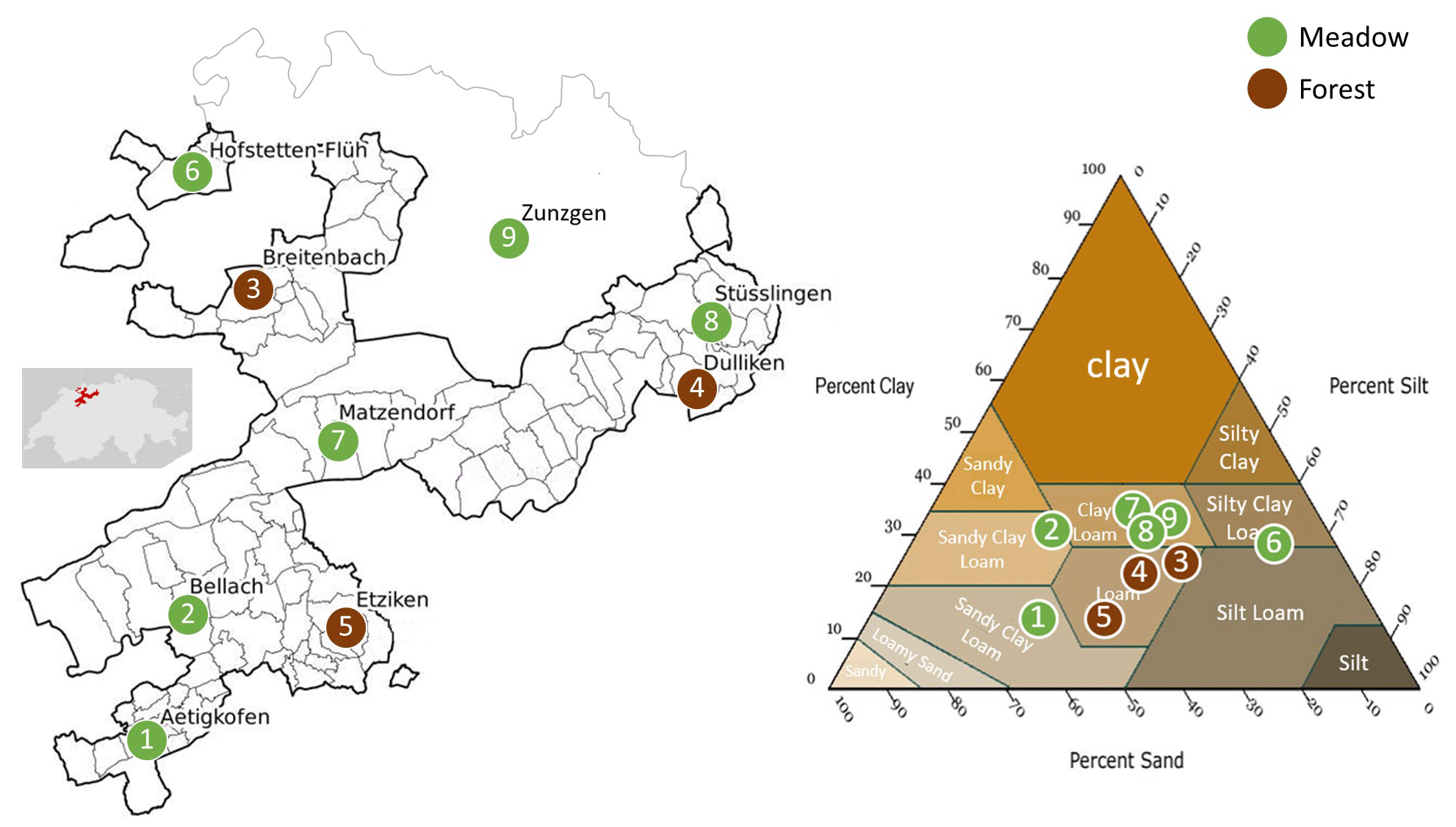
Figure 1 Overview of the study area with site locations, soil texture, and land cover. The primary focus is on the canton of Solothurn, outlined by the black border on the map, with an additional site from the canton of Basel (site 9, Zunzgen). Within this region, three sites are categorized as forests, while the remaining six sites are designated meadows. The analyzed soil horizons (20 cm depth) of the study area encompass five soil textural classes as shown in the soil texture triangle.

The analyzed soil horizons of the selected locations can be assigned to five different soil textural classes (Fig. 1) and two different land cover types (meadow and forest). The Matzendorf location (site 7) contains the highest clay content, whereas locations such as Aetigkofen (site 1) are predominantly sandy. Across these nine locations, different relationships between matric potential and water content were deduced from field data, as shown in Fig. 2 for two sites with low and high variations in water content for similar potential values. To show the relevance of seasonal patterns, we differentiate between summer (April to September) and winter (remaining months).

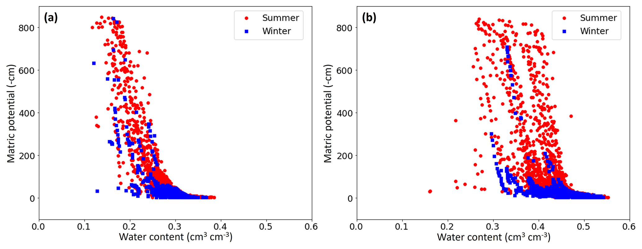
Figure 2 The soil water characteristic curve (SWCC) measured in the field at two sites classified into summer (April to September) and winter (remaining months) from 2012 to 2023. (a) The Etziken site (site 5) shows small changes in the SWCC dynamics over the years, for both the warm and the cold period. (b) A contrasting scenario was found for the site in Bellach (site 2) that was characterized by a wide range of water content for similar potential values. The unit of matric potential, represented in negative centimeters (−cm), is equivalent to −0.1 kPa.

2.2 Deep neural network (DNN)

A basic artificial neural network (ANN) comprises one or two hidden interconnected layers, with each layer tasked with the conversion of an input vector (x) into a hidden state vector (h), as described by Bertels and Willems (2023). This conversion is accomplished with Eq. (1):

$$\begin{array}{}\text{(1)}& \mathit{h}=f\left(\mathit{x}\right)=\mathrm{act}(\mathbf{W}\mathit{x}+\mathit{b}),\end{array}$$

where f(x) represents the transformation function applied to the input vector (x), with a weight matrix (W) and a bias vector (b), integrated with an activation function (denoted “act”).

To construct a deep neural network (DNN), multiple layers (more than two hidden layers) are interconnected to form a “multilayer perceptron”. The training process involves finding optimal values for the weights and biases in the network using suitable optimization techniques (Bertels and Willems, 2023). In this study, a DNN was built to predict the daily MP for the nine sites. The process involved several key steps. First, in the design of the neural network, activation functions were carefully selected and integrated to introduce non-linearity into the model's transformations (Montesinos López et al., 2022). The rectified linear unit (ReLU) activation function was employed to mitigate the vanishing gradient problem and enhance the model's ability to handle noisy input. The inclusion of ReLU was motivated by considerations of computational efficiency, with some attention given to the potential issue of “dying ReLU” (Lu, 2020; Montesinos López et al., 2022).

Next, the neural network was structured with a total of six layers, including four hidden layers as suggested by Achieng (2019). All layers were densely connected, fostering strong information flow between neurons. Crucially, batch normalization was incorporated after the second hidden layer. Batch normalization is a technique that normalizes the activations within a layer during training, which can help mitigate issues like internal covariate shift and accelerate convergence (Ioffe and Szegedy, 2015). The choice of the optimization method was the Adam optimizer, a powerful tool for training neural networks. It adaptively adjusted learning rates, thereby optimizing the learning process and enabling rapid convergence while employing the mean squared error (MSE) as the loss function (Kingma and Ba, 2014). To prevent overfitting by the Adam optimizer, an early stopping mechanism was implemented. This mechanism continuously monitored the loss function for the holdout data during training, ceasing the process if no improvement or a sudden increase was detected over a predetermined number of consecutive epochs.

The initial deep neural networks (DNNs) were configured with four input parameters and the daily logarithmically scaled matric potential (MP) value as output. The input parameters consisted of precipitation, potential evapotranspiration, measured VWC, and the weekly percentage change in VWC. As the prediction process progressed, two major issues were identified. Firstly, the influence of the VWC measurements on the training process was found to be predominant. Consequently, a decision was made to increase the weight of precipitation and potential evapotranspiration in the calculation process by incorporating three new input parameters: the weekly total precipitation and evapotranspiration (the sum of the current day and the preceding 6 d), along with the difference between these two new components. Secondly, the use of logarithmically scaled MP values was found to be highly sensitive to data availability. Therefore, a decision was made to retrain the model using absolute linear MP values (see Appendix B). In total, the final model was equipped with seven input parameters to predict the absolute linear MP values for a given location. For each site, a site-specific DNN was built. The extent of the training data is predominantly influenced by site-specific characteristics. For instance, sites characterized by sandy soils necessitated a shorter training duration in contrast to sites with a higher clay content. Typically, the training dataset spanned a duration of 4 to 7 years. During this period, 70 % of the data were randomly selected for training, while the remaining 30 % were set aside as holdout data (Gholamy et al., 2018). The extra years of data beyond the initial training period were reserved for validation purposes.

2.3 Autoencoder neural network (AUNN)

The autoencoder, consisting of an encoder and a decoder, is an unsupervised deep neural network that learns how to efficiently compress input data into a meaningful representation and subsequently reconstruct the original data from this compressed form (Chen and Guo, 2023). By connecting the encoder and decoder, the autoencoder effectively captures important patterns and variations present in the data, enabling comprehensive analysis and interpretation (Chen and Guo, 2023). In this study, an autoencoder neural network (Fig. 3) was built to analyze the measured VWC time series at 20 cm depth for the nine sites.

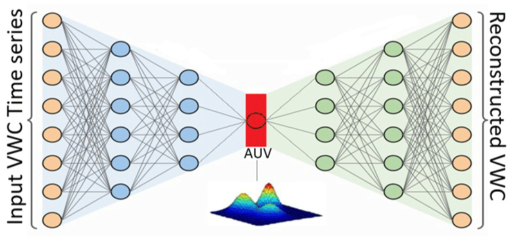
Figure 3 Autoencoder deep neural network for volumetric water content dynamic analysis. In this illustration, a densely connected autoencoder is utilized to compress the dynamic information of volumetric water content (VWC) into a singular value, the autoencoder value (AUV), highlighted in red. The process begins with the encoder, depicted in blue, extracting the AUV from the measured volumetric water content time series (left orange layer). Subsequently, the densely connected decoder, represented in green, utilizes the AUV to reconstruct VWC (orange layer at the right). Both the encoder and decoder, characterized by dense connections, optimized the AUV by minimizing the error between the measured VWC and the reconstructed VWC. The figure was adapted from O'Connor (2022).

The process was as follows. Firstly, an encoder neural network was created for each site. Its objective was to take the VWC time series as input and gradually reduce its dimensionality through hidden layers (Chen and Guo, 2023). The encoders' output was a single site-specific latent representation, called the autoencoder value (AUV), which captures essential features of the VWC dynamics (Chen and Guo, 2023). Subsequently, a decoder neural network was developed to utilize the AUV as a reference to reconstruct the original VWC time series data. The success of this reconstruction depends on the training process, which aimed to optimize the AUV by minimizing the error between the original VWC time series and its reconstructed counterpart by minimizing the mean squared error (MSE) value to less than 0.1.

After the optimization process, for each site one autoencoder value (AUV) was obtained. These AUVs were scaled and then used to build a combined model (Fig. 4) as follows. The AUVs were sorted into three categories. Subsequently, one site from each category was selected. Finally, the data from the three chosen sites, each representing one category, were used to train the combined AUNN–DNN model. The final combined model was thus equipped with eight input parameters to predict the dynamic MP for a specific location. These parameters consisted of the seven inputs employed in the DNN model (Sect. 2.2) complemented by the AUV. The neural network structure, as detailed in Sect. 2.2, remained unchanged, employing the same optimization techniques.

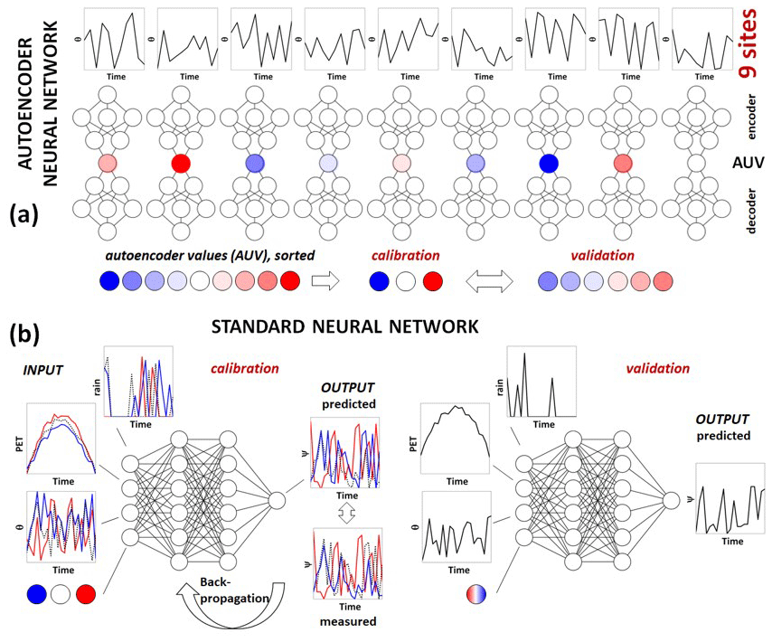
Figure 4 Application of two different types of deep neural networks for the prediction of matric potential ψ. In this conceptual example, the water moisture dynamics of nine sites were considered. (a) The autoencoder neural network captures the characteristic features of the soil water content (θ) dynamics, assigning an autoencoder value (AUV) to each site. These values are sorted into AUV classes (one site from each class was used for calibration and the remaining sites for validation). (b) The combined AUNN–DNN model is built using the calibration sites with the rainfall, potential evapotranspiration (PET), water content, and AUV as part of the eight input parameters. The predicted matric potential (ψ) is compared to measured values for backpropagation. The calibrated DNN is then used to predict ψ for the remaining sites.

Initially, 70 % of the data from each of the training sites were randomly selected for the training dataset. Subsequently, the remaining 30 % of the data were set aside as the holdout dataset, serving as a benchmark for assessing model performance. The developed AUNN–DNN model was then applied to the other six sites (with the same input variables including the AUV) to predict the entire datasets of those unseen sites. The combined model has thus the strengths of both components – the DNN's ability to understand dynamic MP patterns and the feature extraction capabilities of the autoencoder. This shift in the model's strength extends it from being site-specific to encompassing multiple sites, enabling it to gain a broader understanding of how the dynamic MP and AUVs relate to each other.

2.4 Statistical evaluation

The evaluation of model performance is carried out by comparing the model predictions to the measured data. While there is no universal consensus on a standardized evaluation procedure, it is widely recognized that a multi-objective approach should be adopted e.g., Boyle et al. (2000) and Willems (2009). In this study, a combination of four evaluations tools was adopted. First, a scatterplot of observations against simulated values was utilized to visualize the degree of alignment with the identity line (often referred to as the 1:1 line). This graphical approach allowed for a qualitative assessment of model performance. A closer concentration of data points near the 1:1 line indicated higher agreement between calculated and observed values. Moreover, this graphical method includes the 95 % confidence interval area, which helps in scrutinizing the model's consistency across different prediction ranges and detecting potential biases in the model's performance (Ritter and Muñoz-Carpena, 2013). The second criterion evaluates the distribution of (signed) prediction errors (Eq. 2). Ideally, the error distribution should be centered around zero, following a normal distribution pattern around this point with low standard deviation. Such a distribution indicates an unbiased model with errors that tend to balance out. Deviations from this pattern may suggest model bias or other unexpected characteristics in the prediction errors (PEs; den Ouden et al., 2012).

$$\begin{array}{}\text{(2)}& \mathrm{PE}=O_i-P_i,\end{array}$$

with observed O_i and predicted matric potential value P_i. The third evaluation metric was the root mean square error (RMSE; Eq. 3a). RMSE with a value of zero indicates a perfect fit, while a higher RMSE value means worse model performance (Ritter and Muñoz-Carpena, 2013). The final criterion for model evaluation involved the use of the dimensionless goodness-of-fit indicator (Eq. 3b), known as the coefficient of efficiency (NSE; Nash and Sutcliffe, 1970). The NSE, which ranges from negative infinity to 1, serves as an indicator of model performance, with a value of 1 indicating a perfect fit, while a negative NSE suggests that using the means of the observed values is more representative of the data than the evaluated model itself (Gupta and Kling, 2011; Ritter and Muñoz-Carpena, 2013). An NSE value >0.75 indicates a very good model, while an NSE value <0.5 signifies unsatisfactory results (Moriasi et al., 2007). In Gupta et al. (1999), a threshold NSE value of 0.80 was used for good model performance and is applied here as well. The RMSE and NSE are defined by

$$\begin{array}{}\text{(3a)}& {\displaystyle }\mathrm{RMSE}=\sqrt{{\displaystyle \frac{\sum (O_i-P_i{)}^{\mathrm{2}}}{N}}},\text{(3b)}& {\displaystyle }\mathrm{NSE}=\mathrm{1}-{\displaystyle \frac{\sum (O_i-P_i{)}^{\mathrm{2}}}{\sum (O_i-\stackrel{\mathrm{‾}}{o}{)}^{\mathrm{2}}}},\end{array}$$

where O_i represents the measured value, P_i the simulation output, and $\stackrel{\mathrm{‾}}{o}$ the mean of the observed values, all within the context of a sample size N.

3 Results

Following the model discussion in Sect. 2.2 and 2.3, we first present the results of the site-specific tests of predicting matric potential dynamics with a deep neural network (water content, rainfall, and evapotranspiration as input data) before the role of the autoencoder value is considered.

3.1 Deep neural network modeling without an autoencoder

The site-specific DNN model was used to simulate the time series for all nine sites. In Fig. 5, the results are shown for the Stüsslingen site (site 8, clay loam, meadow). The model was trained on data that had 1825 d of observations from January 2012 to January 2018. The data were split randomly into two parts: (1) a calibration dataset that had 1277 d and (2) a holdout dataset that had 548 d. The model was then validated on data from February 2018 to January 2023 (1379 d). A strong agreement between the model and the observed data was discovered in both the training and the validation datasets (Fig. 5c), as reflected by the low RMSE value and the high NSE value (Table 1). Furthermore, it was noticed that the error distribution exhibited a predominantly normal pattern with minimal bias towards higher observed values compared to the predicted values (Fig. 5d). These findings suggest that the site-specific DNN model not only was able to be well generalized to unseen data but also demonstrated a reliable ability to predict MP.

The statistical evaluation (Table 1) reveals a consistent performance across both the training and the validation periods for the Stüsslingen site, offering compelling evidence that the model avoids overfitting. Additionally, when it comes to predicting MP values, the 95 % confidence interval indicates that the model can capture the overall dynamics well (Fig. 5b). However, the model performance exhibits higher deviations for values exceeding 400 cm and consistently underestimates values higher than 600 cm (Fig. 5b), which could explain the mild positive skewness observed in the distribution of prediction errors in Fig. 5d.

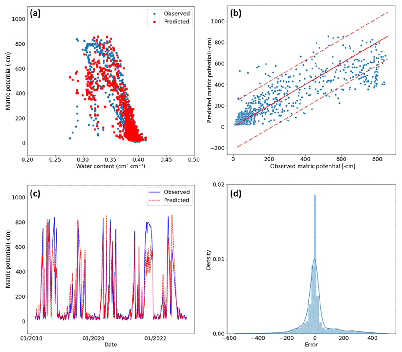
Figure 5 Graphical evaluation of the performance of the site-specific deep neural network (DNN) for validation for the Stüsslingen site (site 8) for the validation period 2018 to 2022. (a) Comparison between the simulated and measured soil water characteristic curve. (b) Scatterplot comparing simulated and measured matric potential values, providing a visual representation of the level of conformity to the identity line. The two dashed lines represent the 95 % confidence interval around the identity line, providing a visual assessment of the level of agreement. (c) Model validation presenting time series with the observed and predicted matric potential. (d) Analysis of the distribution of prediction errors (observed minus predicted values) with a mildly positively skewed distribution.

Comparing the performance for the “holdout” period (randomly chosen days between 2012 and 2019) of the nine site-specific DNN models, the NSE index is larger than 0.55 (“good”) for all sites and larger than 0.80 (“optimal”) for six sites. For all sites, it was thus possible to build a DNN model with good model performance for the randomly chosen test days. However, for the validation period, only four showed optimal performance (NSE >0.80). For two forest sites with an optimal performance for the holdout period (Dulliken, site 4, and Etziken, site 5), NSEs dropped from a range between 0.82 and 0.88 to a range between 0.73 and 0.75 (Table 1). Obviously, the model captured the overall short-term dynamics during training (randomly chosen days) but faced problems in the precise prediction of the long validation period. An extended training period may be necessary to enhance the model's accuracy for these specific sites. Three grassland sites (Bellach, site 2; Matzendorf, site 6; and Hofstetten-Flüh, site 5) showed good but not optimal performance even during the holdout period. As discussed in the next section, this may be related to large variations in the pressure values for similar water content values and the correspondingly large AUV. Notably, the lower performance observed in the holdout period for Hofstetten-Flüh could also be linked to data limitations, as only 1200 d was used to train the model for this specific site (compared to 1825 d for the other sites).

Table 1 Statistical assessment of calibration (1825 d, until the year 2018/2019/2020) and validation (years 2018/2019/2020 until years 2020/2021/2022) results for nine sites. The holdout dataset was part of the training period and includes 548 d (30 % of calibration).

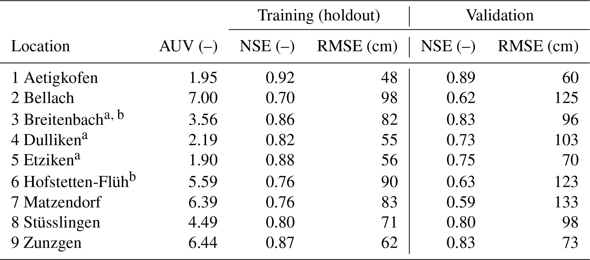
^a Forest sites. ^b Sites with limited available data. For those sites, only 1200 d was used for training. Within this training period, a subset of 360 randomly selected days was designated a holdout dataset; the validation period for those specific sites was from 2018/2019 to 2022.

3.2 Autoencoder DNN

The autoencoder values (AUVs) deduced from the time series analysis of the volumetric water content for the period of 2012–2022 can be classified into three main groups (Fig. 6). Soil water characteristic curves (SWCCs) with low water content in saturated conditions and a small variation in water content for similar potential values are assigned to “type 1”, contrasting “type 2” with large water content values and variations. These types of SWCCs are related to small (type 1) and high (type 2) autoencoder values (AUVs). Sites with AUVs between these two classes are denoted “transitional type” sites in the following. As shown in Table 1, the AUVs of forest soils are small (mainly type 1) with large NSE values. In contrast to the forest soils, there are grassland sites with high AUVs (type 2) but small NSEs. The high variations in the SWCC for type 2 probably require longer training periods to capture the high variations in the pressure–saturation relationship.

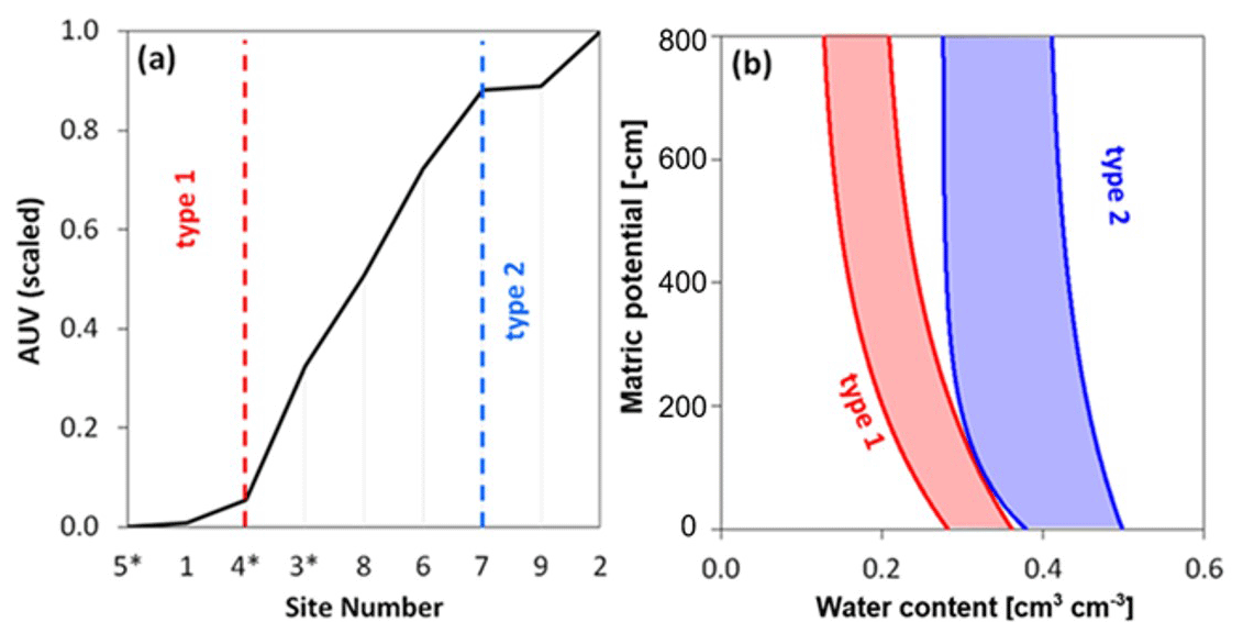
Figure 6 The autoencoder value (AUV) and its relation to the soil water characteristic curve (SWCC). (a) The AUVs of the nine sites with three sites with small (type 1) and three sites with high (type 2) AUVs. (b) The SWCC for type 1 has lower water content near saturation and a narrower range of water content compared type 2, which has higher water content values and more variation. Type 1 shows the data range of Aetigkofen (site 1) and type 2 that of the Bellach site (site 2). The site numbers are chosen in alphabetical order and as shown in Fig. 1 (Aetigkofen (1), Bellach (2), Breitenbach (3), Dulliken (4), Etziken (5), Hofstetten-Flüh (6), Matzendorf (7), Stüsslingen (8), Zunzgen (9); sites with forest are marked with ^*).

3.3 Deep neural network using the autoencoder value (AUNN–DNN)

As mentioned in the previous section, the nine sites could be grouped into three main types according to the scaled autoencoder value (AUV). Consequently, it was assumed that the creation of a DNN model, which incorporates AUVs in conjunction with the previously built site-specific neural network, could enable predictions for unseen sites. Ideally, the model should be trained with a balanced dataset, including one site from the type 1 category, one site from the type 2 category, and a few sites from the transitional category to capture the full transition between type 1 and type 2. However, due to the data limitation, the model was trained for only three sites representing the three types (Etziken, site 5, for type 1; Bellach, site 2, for type 2; Stüsslingen, site 8, for the transitional type) and was then used to predict the six unseen sites. The impact of the small training set (only one site for the transitional type) was clear in the model results, which exhibited some instability, changing from one run to another as the model was not able to assume the same transitional function between sites consistently. Therefore, the model was run 20 times, and then the average result for these runs was taken as a representative outcome. The application of the new DNN model with AUVs to predict the dynamics of matric potential is shown in Fig. 7 for Breitenbach (site 3, loam, forest) as an unseen site. The model was found to fall slightly behind the previously designed DNN model, but it can still predict the dynamics in a good way. Notably, the NSE value for this model for the Breitenbach site was 0.71 over the entire period from 2012 to 2022 (Table 2).

Table 2 AUNN–DNN model performance for the period of 2012–2022. Three training sites were used to build the AUNN–DNN model, which was then applied to the other six sites. The sites are listed according to their corresponding autoencoder value (AUV).

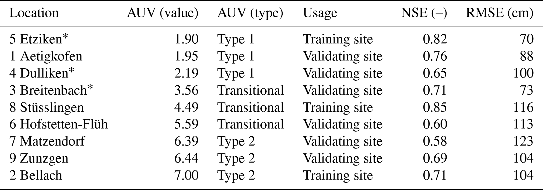
The asterisks mark the sites with forest. The AUV was scaled from 1.9 to 7.0 to simplify input. Alternatively, scaled values ranging from 0 to 1 could also be utilized.

It was noticed that the error distribution exhibited a predominantly normal pattern with a bias towards higher observed values compared to the predicted values (Fig. 7d). The analysis indicates the model's proficiency in forecasting dynamic trends rather than precise values (Fig. 7c). The results align with the anticipated scenario as the AUV for Breitenbach (3.56) was relatively close the Stüsslingen AUV (4.49). Therefore, the underestimation detected in Stüsslingen for the site-specific DNN (Fig. 5b) is expected to exist in Breitenbach as well. The average model performance for all sites is presented in Table 2. The NSE values were >0.55 for the six unseen sites (validating sites) and provided strong evidence that the model can be relied upon for the dynamic MP predictions.

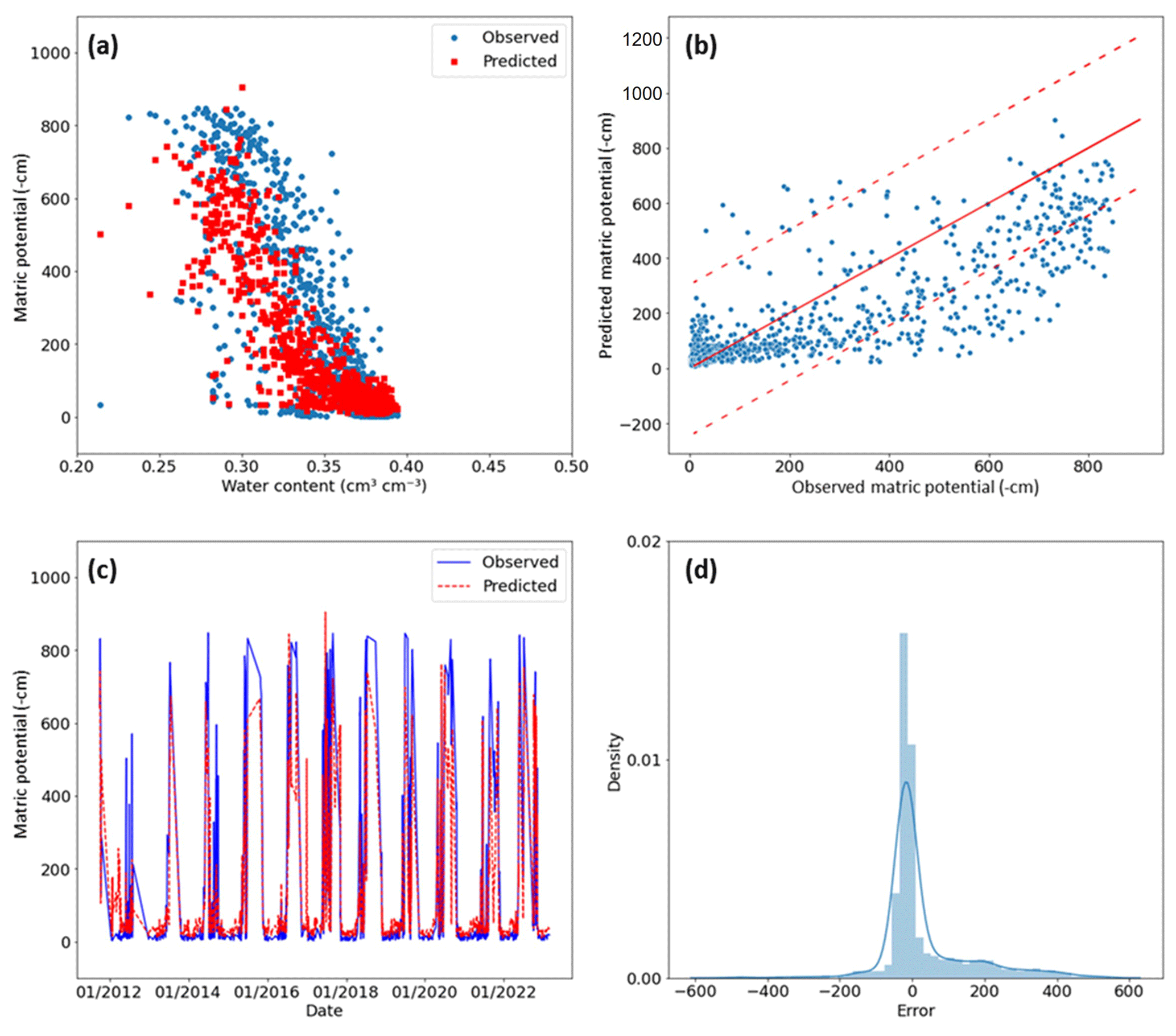
Figure 7 Evaluation of the deep neural network with autoencoder (AUNN–DNN) model performance at the Breitenbach site for the period of 2012–2022. (a) Comparison between the expected soil water characteristic curve (SWCC) and the observed SWCC. (b) Scatterplot that compares observed data points with their corresponding simulated values, providing a visual representation of the level of conformity to the identity line. The two dashed lines represent the 95 % confidence interval around the identity line, providing a visual assessment of the level of agreement. (c) Time series comparison showing the observed and predicted matric potential for the entire period. (d) Analysis of the distribution of prediction errors (observed minus modeled value) using a mildly positively skewed distribution.

The NSE values for the unseen sites (validating sites) varied from 0.58 to 0.76, indicating a spectrum of model performance that ranged from acceptable to good. The low NSE values observed for Matzendorf (site 7) suggest that the model's utility is more suited for capturing overall trends and dynamics rather than precise values. This evaluation was further supported by examining scatterplots (Fig. 8) that compare the observed data points with their corresponding simulated values for the sites that scored the lowest and the highest NSE, Matzendorf (site 7) and Aetigkofen (site 1). The plots reveal a wider 95 % confidence interval for Matzendorf (Fig. 8a) in comparison to Aetigkofen (Fig. 8b), indicating that the lower the NSE value is, the more challenging it becomes for the model to predict the exact MP values. However, the model performance indicated the ability of the AUNN–DNN model to predict dynamic MP without the necessity of site-specific training data, marking a transition from the DNN site-specific nature to a more versatile multisite model.

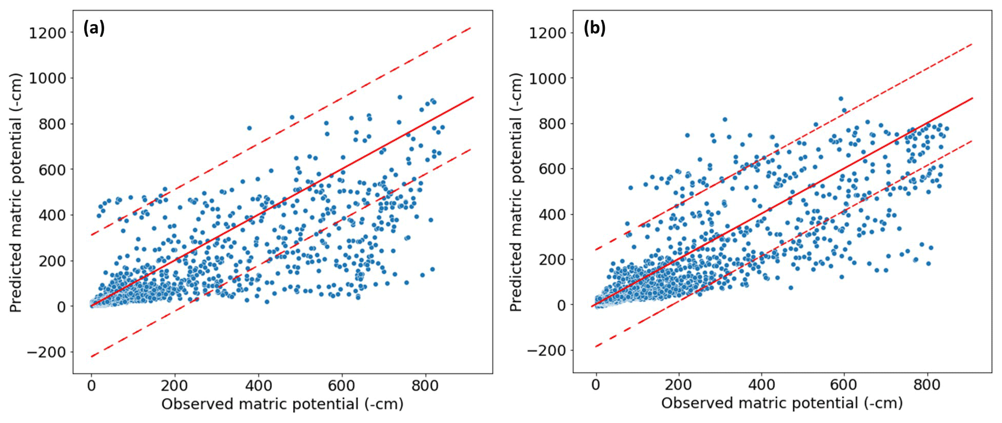
Figure 8 Comparison between observed data points and their corresponding simulated values for two sites with the lowest and highest efficiency coefficient (NSE). (a) Matzendorf (site 7) with an NSE of 0.58. (b) Aetigkofen (site 1) with an NSE of 0.76. The solid lines mark the 1:1 correspondence and the dashed lines the 95 % confidence interval.

4 Discussion

Based on the analysis of the simulation results presented in Sect. 3, it can be asserted that the model was successfully built. However, as discussed in the next subsection, the model is expected to have certain drawbacks due to the limited number of available sites. In the other subsections that follow, the relationship between the autoencoder value and soil properties and its application to satellite data will be discussed.

4.1 Limits of the deep neural network with an autoencoder value (AUNN–DNN)

First, the model's statistical evaluation revealed that the matric potential (MP) at a depth of 20 cm could be simulated with acceptable precision. However, a high variability in the evaluation is indicated by the NSE values for the unseen sites. This variance is attributed to the model's limited generalization capacity, as it was trained on just three sites. Furthermore, the model was not able to capture the entire dynamics for the training sites due to the limited length of available data. For example, Bellach (site 2), a training site that has a high AUV, had an NSE value of 0.71 for the training period (Table 2), which indicates that the model was able to capture the general trend for this site but still could not predict the exact value of the MP. The effect of this result on the sites that are close to the AUV type 2 category (i.e., Hofstetten-Flüh and Matzendorf, sites 6 and 7, with NSEs of 0.60 and 0.58, respectively) was obvious.

The stability of the AUNN–DNN model was insufficient, as the model showed different prediction quality levels upon running the model repeatedly for the same training sites (Fig. 9). This variability in the outcomes indicates that the model can find different scenarios of MP dynamics within the training data. Therefore, training the model for more than one site with the same AUV type is recommended.

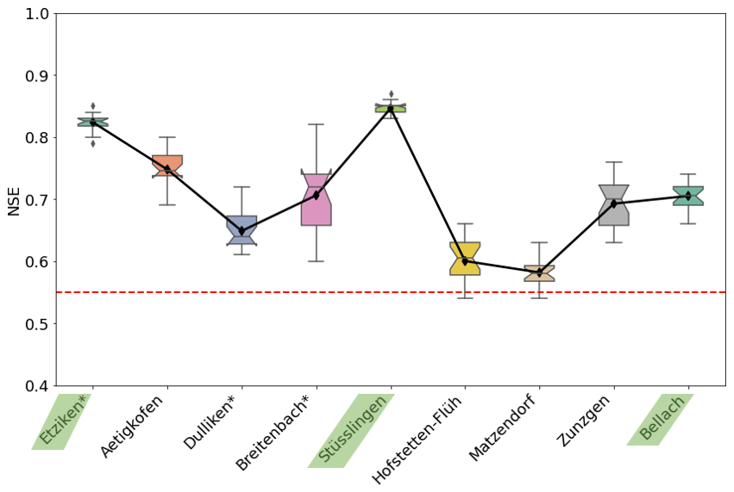
Figure 9 Variation in prediction results for 20 runs for the AUNN–DNN model quantified with the efficiency coefficient (NSE). The highest variation was with the unseen sites in the transitional and type 2 categories. Each box represents the interquartile range, with the line inside denoting the median. The black line with diamond markers connects the mean values for each station, providing insight into the central tendency of the data. Notches on the boxplots offer a visual indication of the uncertainty around the median. The dashed red line represents the defined threshold for the NSE, set at 0.55. Sites with forest are marked with ^*. Training sites are highlighted in green.

Especially for the transitional type, choosing a site at the beginning, in the middle, and at the end of the range defining the category would stabilize the modeling results. However, in this study, there was no possibility of providing the model with extra data to solve the prediction instability. Therefore, a solution was implemented by (1) closely monitoring the model manually to ensure it captures the dynamics from all three sites. This involved training the model with nearly identical time periods for each site and visually confirming comprehensive coverage of the cloud of points for the retention curve of each site, avoiding concentration of specific patterns during training. The process also includes (2) running the model 20 times and then averaging the results. Additionally, statistical evaluation plots, as shown in Fig. 8, were used to detect instances with very low or very high MP prediction values.

For the set of sites analyzed in this study, the model showed good generalization capacity and stability. However, the nine sites were similar with respect to climate and geology, and the range of soil textural classes (see Fig. 1) was relatively narrow. In a future study, the AUNN approach will be applied to sites differing in climate and soil textural classes. We expect that the model will be able to predict the dynamic matric potential for a new site as long as the autoencoder value falls within the range of the AUVs of the training sites. To predict the soil moisture dynamics for soils with autoencoder values outside of the range of training data, the model must be re-built using additional training data.

4.2 Interpretation of the AUV and its relationship to physical soil properties

As discussed in Sect. 3.2, the autoencoder value (AUV) is low for soil water characteristic curves (SWCCs) with low saturated water content and low variations in water content for a certain matric potential value (type 1) and high for large values of and variations in water content (type 2). To provide a more quantitative relationship between the SWCC and AUV, the SWCC data were characterized as follows: the time averages of the volumetric water content (VWC) and soil water potential (SWP) were calculated for 15 d for the period of 2015 to 2022. The envelope of these data was then calculated by fitting a minimum and maximum pressure–saturation relationship that included the averaged data (see Fig. 10a).

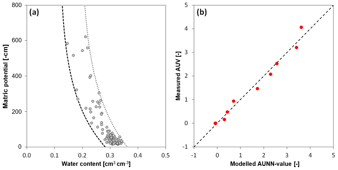
Figure 10 Relationship between the autoencoder value (AUV) and soil water characteristic curve (SWCC). (a) The 15 d average of SWCC data for Aetigkofen (symbols; site 1). The two lines are exponential functions that form the envelope of the SWCC. (b) The linear model for the nine sites linking the parameters of the exponential model with the “measured” AUV (deduced from measured water content data).

The two boundary lines of the SWCC were then characterized by a “saturated” and “residual” water content and a shape parameter defining an exponential decrease in water content with increasing absolute matric potential values. The SWCC of each site can thus be described by six parameters (three parameters per boundary line). As shown in Fig. 10b, a linear model expressing the AUV as a function of these six parameters can be built. Simpler models with fewer parameters could not reproduce the AUVs of all sites. Despite the positive correlation between AUVs and average water content, the average water content alone is not sufficient to explain the range of AUVs for all sites. Combining average water content with soil texture information could also not reproduce the AUVs of all sites, indicating that the soil moisture dynamics represented by the AUV is dependent on not only static soil textural attributes but also seasonal structural features.

Accordingly, there is no simple interpretation of the AUV based on texture and average water content, but the dynamic variation in water content must be considered as well. Due to the relevance of the variation in water content for similar matric potential values, the use of a variational autoencoder (VAE) instead of the typical autoencoder could be considered. In contrast to the typical autoencoder, which maps the input information into a single point (or a few points), the VAE produces a probability distribution that captures the variability (second moment) in the data. This could be specifically of interest for clay soils with high water content (much larger than the residual water content) for the entire range of matric potential values. By including a probabilistic approach in the compressing and decompressing step, the variability in the data could be captured more efficiently using a VAE.

4.3 Application to satellite data

The AUNN–DNN model was used to analyze satellite-based volumetric water content (VWC) satellite data, including SMAP (Soil Moisture Active Passive) Level 4 (L4) and Level 3 (L3) products, SMOS (Soil Moisture and Ocean Salinity) products, and Sentinel data. Subsequently, a comparison was carried out for the AUV for both site-specific measurements and earth observation (EO) measurements for the same region. The initial findings highlighted a disparity between the dynamics captured by EO products and the actual dynamics. Therefore, if the objective is to establish a robust system capable of detecting changes in water retention dynamics on a regional scale, it is considered necessary to enhance the calibration of EO in Europe. Only with EO data that can reproduce the essential part of the soil moisture dynamics as manifested in the AUV can the matric potential dynamics be deduced from EO data. For future EO data with improved capacity to capture regional soil moisture dynamics, the concept presented in this study (AUNN–DNN) could be used to predict matric potential dynamics at the global scale (see Appendix C).

5 Summary and conclusions

The soil water potential (SWP) determines the water flow direction, water availability for plants, and mechanical stability. Because it cannot be measured directly by remote sensing techniques at larger scales, it is often deduced from water content information, assuming an unambiguous relationship between water content and SWP. However, this relationship under dynamic field conditions is highly ambiguous due to hysteresis, dynamic effects, and soil structural changes that cannot be modeled with a physically based model. To enable prediction of SWP from soil water content, we apply a deep neural network (DNN) with an autoencoder to define unique features of the soil moisture dynamics. By inserting the autoencoder value (AUV) together with climatic data and water content measured at nine sites in the region of Solothurn (Switzerland) in a deep neural network (AUNN–DNN), the soil water potential could be predicted. The main findings of the study can be summarized as follows:

• The SWCCs of the nine sites can be classified into three types based on the width of the pressure–saturation relationship and the water content close to saturation.

• These SWCC types are manifested in different autoencoder values (AUVs).

• The AUV not only is a simple function of average water content or soil texture but also includes structural effects.

• The AUNN–DNN model could successfully predict the SWP dynamics of sites without site-specific training.

The autoencoder value (AUV) is thus a new descriptor of the complex soil moisture dynamics that cannot be captured with physically based models. Future satellite generation may be sensitive enough to measure the AUV from remote sensing water content data. The approach presented in this paper will then enable the prediction of the soil matric potential at the global scale using remote sensing water content data.

Appendix A: Data quality assurance and trend analysis

As a precaution for data quality, the absolute matric potential (AMP) and volumetric water content (VWC) data were scrutinized to identify potential errors in the data. The process includes different steps that were necessary to discover anomalies, checking the integrity of the data and detecting systematic changes with time.

A1 Flagging abrupt changes in VWC and MP

• VWC flagging and removing.

  Differences between consecutive (daily) time steps in the water content time series were calculated.

• Instances with daily differences exceeding 0.1 cm³ cm⁻³ were flagged and termed sudden decreases or increases in VWC.

• Instances with VWC below 0.1 cm³ cm⁻³ or exceeding 0.7 cm³ cm⁻³ were identified and removed from the dataset. These extreme values were considered measurement anomalies or outliers affecting the overall dataset's reliability.

• Instances with AMP <1 cm were removed from the data to overcome limitations in the method used. The water potential can change without modifying the volumetric water content after this limit, which could make the results of the model not accurate enough.

• The differences between consecutive time steps in AMP time series were calculated; instances with daily differences exceeding 500 cm were flagged and called sudden decreases or increases in AMP (Fig. A1).

• The threshold AMP value of 850 cm was employed in a specific step, where instances with AMP exceeding 850 cm were removed from the dataset, addressing the physical properties of water as it starts to boil in the tensiometers under pressure after this limit.

• Periods of a concurrent decrease in AMP (indicator for wetting) and decrease in VWC (drying) were flagged (Fig. A1).

• Periods with matric potential values remaining constant over a 3 d rolling window were flagged (Fig. A1).

A2 Utilizing index windows for data manipulation and data removal

To address the flagged instances mentioned before, a systematic approach is employed. For each flagged instance, three additional indices are generated around it to construct an index window, spanning 1 d before the instance (index_1), the flagged instance itself (index_0), and 2 d after the instance (index_2 and index_3). This 4 d index window was eliminated from the dataset (Fig. A1). The decision to eliminate this window was informed by a visual assessment of measurements as it was noticed that when a measurement error occurs, the accuracy of the preceding day is affected. Furthermore, it was assumed that the device requires 2 subsequent days to restore normal measurement precision. This process contributes to a refined dataset, providing a more accurate representation of the underlying trends in AMP and VWC.

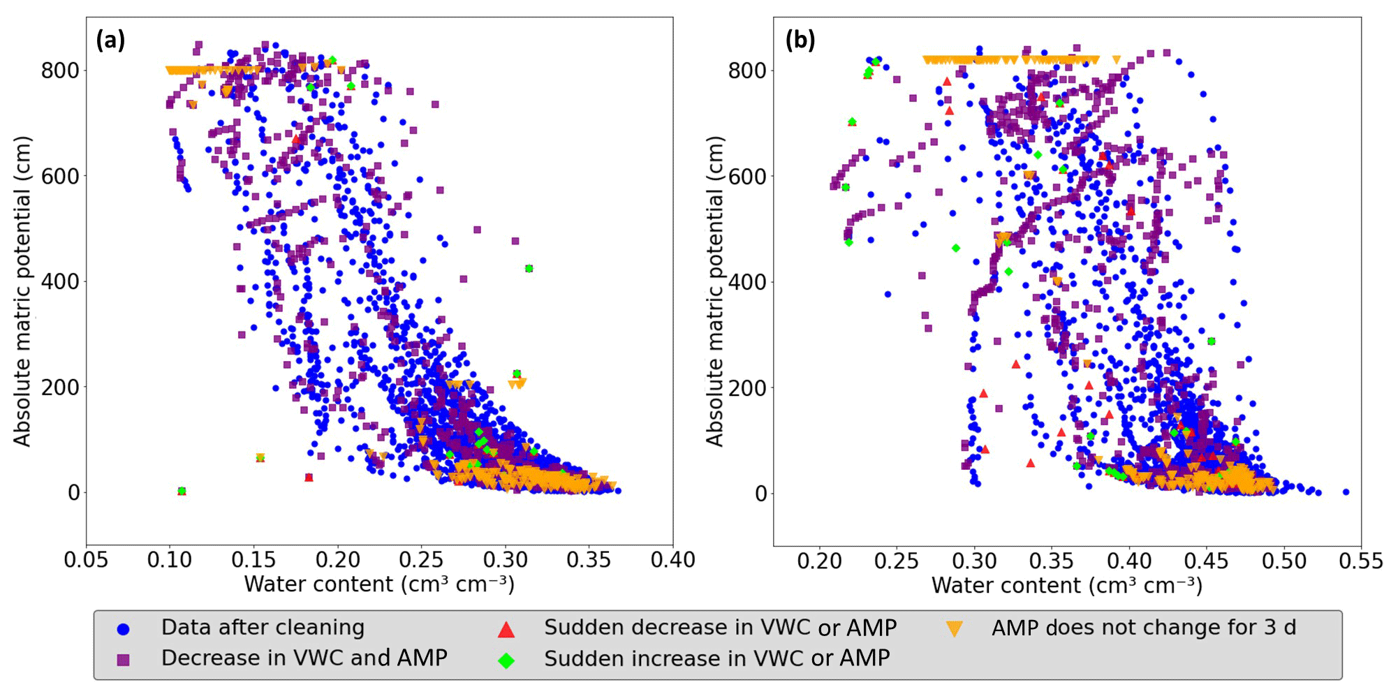
Figure A1 Comparison of data before and after the cleaning procedure: the blue circles depict the remaining data after applying the cleaning criteria. Each distinct marker represents eliminated points, with each corresponding to a specific criterion (i.e., the square purple marker for a simultaneous decrease in volumetric water content (VWC) and the absolute matric potential (AMP), the red upward-pointing triangle is the marker for sudden decreases, the lime diamond is for sudden increases, and the orange downward-pointing triangle marks periods of unchanged AMP). This provides insights into the reasons for data removal and illustrates the profound impact of the data cleaning process in retaining high-quality data points. In (a) the cleaning process for the sandy clay loam site in Aetigkofen (site 1) is shown, and in (b) the cleaning process for the Matzendorf site (site 9, clay loam soil) is shown.

Appendix B: Running the model with a logarithmic MP value

AUNN–DNN showed a good performance in predicting the dynamic MP for the six different unseen sites. However, it was clear that the model tends to focus on capturing significant changes in values rather than accurately representing the values themselves. This tendency is attributed to the substantial difference between the highest and lowest absolute values (approximately 850 cm), leading the model to emphasize major fluctuations while neglecting minor ones. To address this issue and enhance the model's precision in capturing the exact AMP, a suggestion has been made to train the model for the same three sites but with the logarithmic value for AMP. This modification aims to strike a better balance, ensuring that both major and minor changes are effectively captured while maintaining accuracy in representing the specific values of MP.

To qualitatively assess the model training performance on the logarithmic scale, scatterplots (Fig. B1) were generated that compare observations against simulated values for the second training site (Stüsslingen). The reason for choosing a training site was to understand how the model captures the dynamics when trained with the logarithmic matric potential. The results suggest that using a logarithmic scale, the model prioritized the prediction of the exact value of absolute matric potential (AMP), which made the model optimize predictions for the absolute values between 0 and 200 cm. This approach gives the same importance to small and large changes in AMP, which causes the model to assign a higher weight to small changes according to their higher frequency and neglect less frequently occurring major dynamic shifts. Consequently, the model's accuracy went down beyond 200 cm (Fig. B1a) when compared to the model trained on non-logarithmic AMP values (Fig. B1b). To maintain a balanced consideration of changes, logarithmic MP was avoided in the main part of the paper.

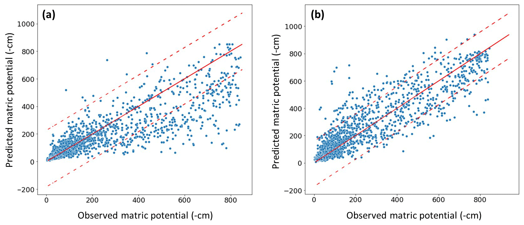
Figure B1 Visual comparison of model performance, comparing the observed and simulated values for the Stüsslingen training site. (a) The model trained with logarithmically scaled AMP values. (b) The model trained with linear absolute matric potential (AMP) values. The solid line denotes the 1:1 correspondence, and dashed lines represent the 95 % confidence interval.

Appendix C: SMAP data and autoencoder for global-scale analysis

SMAP (Soil Moisture Active Passive) is a NASA satellite mission that was established to help improve weather forecasts and global drought monitoring. SMAP data products are available at different levels of processing, from Level 1 (L1; instrument measurements) to Level 4 (L4; model-derived value-added products). For this study, SMAP L3 and SMAP L4 products for measuring moisture content were used. The main difference between the two product types is that SMAP L3 products depend on the passive radiometer measurements, while SMAP L4 products are derived from a data assimilation system that combines the L-band brightness temperature observations from SMAP with a land surface model and meteorological forcing data (Reichle et al., 2019). SMAP L3 products for moisture content are primarily affected by vegetation and surface roughness, allowing them to capture surface soil moisture variations. In contrast, the incorporation of land surface models into SMAP L4 products reduces its sensitivity to vegetation cover types and surface roughness, making the products more representative of the profile soil moisture conditions (Reichle et al., 2019).

The autoencoder's encoded representations offer a unique opportunity to compare the spatial patterns inherent in “point measurement” with remote sensing data such as SMAP L3 and SMAP L4 data. The autoencoder method could illuminate how these diverse data streams align or diverge, providing crucial insights into the compatibility and complementarity of ground and satellite measurements. The process was applied for the data between the years 2015 and 2022. All the data (SMAP L4, SMAP L3, and on-site measurements) were given to the autoencoder neural network together. Subsequently, the resulting autoencoder values were scaled. Finally, a comparison was made to show whether the satellite measurements and the on-site measurements had the same measured dynamics.

The autoencoder analysis of SMAP L3 (Fig. C1) indicates that satellite measurements struggle to capture the dynamic change in the water content, as all locations yield approximately the same autoencoder value (AUV). In contrast, the SMAP L4 product (Fig. C1) exhibits fluctuations in AUV results. For instance, Stüsslingen and Matzendorf align closely with on-site measurements in terms of AUVs. However, for Hofstetten-Flüh, the SMAP L4 product indicates a very small AUV, suggesting an expected dynamic in line with a type 1 soil water retention curve (Fig. 6b). In contrast, on-site measurements indicate a higher AUV for Hofstetten-Flüh, suggesting a closer association with a type 2 soil water retention curve. These findings underscore the need to develop a new methodology to calibrate satellite data in the Switzerland area. The prevalent uniformity in SMAP L3 results and the notable disparities between on-site measurements and satellite data across various products highlight the need for a more refined approach to ensure accurate and reliable dynamic soil moisture assessments.

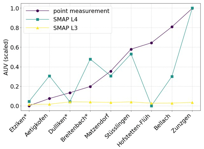
Figure C1 Comparative analysis of autoencoder neural network results for SMAP L3 and SMAP L4 satellite data, alongside profile measurements. The fluctuating AUVs indicate varying degrees of alignment with on-site measurements across different locations. Sites with forest are marked with ^*.