the Creative Commons Attribution 4.0 License.
the Creative Commons Attribution 4.0 License.
 | 12 Sep 2024
Regionalization in global hydrological models and its impact on runoff simulations: a case study using WaterGAP3 (v 1.0.0)
Nina Kupzig
Martina Flörke
Valid simulation results from global hydrological models (GHMs), such as WaterGAP3, are essential for detecting hotspots or studying patterns in climate change impacts. However, the lack of worldwide monitoring data makes it challenging to adapt GHM parameters to enable such valid simulations globally. Therefore, regionalization is necessary to estimate parameters in ungauged basins. This study presents the results of regionalization methods for the first time applied to the GHM WaterGAP3. It aims to provide insights into (1) selecting a suitable regionalization method for a GHM and (2) evaluating its impact on runoff simulation. In this study, four new regionalization methods have been identified as appropriate for WaterGAP3. These methods span the full spectrum of methodologies, i.e., regression-based methods, physical similarity, and spatial proximity, using traditional and machine-learning-based approaches. Moreover, the methods differ in the descriptors used to achieve optimal results, although all utilize climatic and physiographic descriptors. This demonstrates (1) that different methods use descriptor sets with varying efficiency and (2) that combining climatic and physiographic descriptors is optimal for regionalizing worldwide basins. Additionally, our research indicates that regionalization leads to spatially and temporally varying uncertainty in ungauged regions. For example, regionalization highly affects southern South America, leading to high uncertainties in the flood simulation of the Río Deseado. The local impact of regionalization propagates through the water system, also affecting global estimates, as evidenced by a spread of 1500 km3 yr−1 across an ensemble of five regionalization methods in simulated global runoff to the ocean. This discrepancy is even more pronounced when using a regionalization method deemed unsuitable for WaterGAP3, resulting in a spread of 4208 km3 yr−1. This significant increase highlights the importance of carefully choosing regionalization methods. Further research is needed to enhance the predictor selection and the understanding of the robustness of the methods on a global scale.
- Article
(7035 KB) - Full-text XML
- BibTeX
- EndNote


Global hydrological models (GHMs) are developed and applied worldwide, e.g., to detect hotspots and examine patterns of climate change impacts on the terrestrial water cycle (Barbarossa et al., 2021; Boulange et al., 2021). Valid model results are a prerequisite for drawing robust conclusions. For valid modeling results, it is beneficial to adjust the parameter values to adapt the models to different basin processes (Gupta et al., 1998). This adaptation is usually modified and evaluated (in a loop) by comparing the simulated model output, often discharge, with the monitored data. However, this parameter adjustment for GHMs is challenging due to the lack of global monitoring data. Consequently, parameter adjustment for GHMs can be based not only on monitored data (i.e., calibration) but also on the estimation of parameter values for ungauged basins (i.e., regionalization).
Regionalization defines the estimation of model parameters for ungauged basins (Oudin et al., 2008), usually based on information from gauged basins (Oudin et al., 2010). Regionalization methods generally follow the same principle: basin characteristics (e.g., physiographic and/or climatic) are linked to hydrological characteristics and can thus be used to estimate parameter values. Various regionalization methods exist, and no overall preferred method has been found (Ayzel et al., 2017; Pool et al., 2021). In contrast, the optimal regionalization method may differ, for example, regarding available information (Pagliero et al., 2019) or model structures (Golian et al., 2021). Therefore, different methods should be tested to find an optimal regionalization method for a specific use case (e.g., Qi et al., 2020).
Evaluation is needed to assess different regionalization methods. The evaluation of regionalization methods is particularly challenging because they are usually applied when there is a lack of monitoring data. Therefore, regionalization studies often treat gauged basins as ungauged and perform leave-one-out cross-validation (e.g., Chaney et al., 2016) or split-sample tests (e.g., Beck et al., 2016; Nijssen et al., 2000; Yoshida et al., 2022). While at the mesoscale, this evaluation is already an integral part (e.g., McIntyre et al., 2005; Parajka et al., 2005; Oudin et al., 2008; Yang et al., 2020), but this is sometimes not the case in global or continental studies (e.g., Müller Schmied et al., 2021; Widén-Nilsson et al., 2007). Another reasonable evaluation strategy is the concept of a benchmark to beat (Schaefli and Gupta, 2007; Seibert, 2001). Applying a benchmark to beat supports a comprehensive evaluation of whether a new approach is functional, e.g., better than a straightforward and thus transparent method or better than a predecessor. To the authors' knowledge, such a benchmark to beat has never been used to evaluate innovations in regionalization at a global scale.
In general, regionalization methods can be divided into two categories based on the parameter estimation strategy: (1) regression based and (2) distance based (He et al., 2011). Regression-based methods derive the relationship between basin characteristics and model parameters through fitted regression models. These mathematically defined relationships are further applied to estimate model parameters of ungauged basins (e.g., Kaspar, 2004; Müller Schmied et al., 2021). A significant drawback of regression-based regionalization is the difficulty of incorporating parameter interdependencies (Poissant et al., 2017), as regression-based approaches often assume that the dependent variables, i.e., the model parameters, are not correlated (Wagener et al., 2004). Distance-based approaches transfer complete parameter sets from similar or nearby donor basins to ungauged basins (e.g., Beck et al., 2016; Nijssen et al., 2000; Widén-Nilsson et al., 2007). Using an ensemble of donor basins, e.g., by averaging the parameter values or model outputs, can improve the performance of such methods (e.g., Arsenault and Brissette, 2014). A significant disadvantage of such methods is the clustering problem of ungauged basins, i.e., the unequal distribution of gauging stations worldwide (Krabbenhoft et al., 2022). Thus, basins exist where distance-based approaches will use non-comparable basins to transfer parameter values due to the lack of close basins.
Recent advances have implemented machine-learning-based techniques in the context of regionalization. For example, Chaney et al. (2016) used regression trees as an alternative to least-squares regression to estimate parameter values in ungauged basins. Pagliero et al. (2019) explored supervised and unsupervised clustering methods to define the similarity of basins to transfer parameter sets. To the authors' knowledge, no study has compared several traditional regionalization methods with machine-learning-based methods for a GHM on a global scale.
Some regionalization methods do not make a clear distinction between calibration and regionalization. For example, Arheimer et al. (2020) applied a basin grouping beforehand. Then, they jointly calibrated the group members to define representative parameter sets. Subsequently, the representative parameter sets are transferred to other basins based on grouping rules. Another approach defines so-called transfer functions (Samaniego et al., 2010) and calibrates meta-parameters instead of the model parameter values (Beck et al., 2020; Feigl et al., 2022). These methods, where regionalization is part of the calibration process, often require a change in the calibration process itself, which is challenging for GHMs (Schweppe et al., 2022) due to, for example, a lack of code flexibility (e.g., Cuntz et al., 2016).
This study proposes an improved regionalization method for the state-of-the-art GHM WaterGAP3 (Eisner, 2016). It compares traditional regionalization methods with machine-learning-based methods and uses a benchmark to beat and an ensemble of split-sample tests to evaluate the applied methods. Further, global runoff simulations are compared to analyze the impact of regionalization methods. The overall research topic is evaluating and selecting regionalization methods for a GHM. Specifically, the study has two objectives. It aims
-
to propose an improved regionalization method for WaterGAP3 and
-
to evaluate the impact of regionalization methods on global runoff simulations.
2.1 The model: WaterGAP3
The GHM WaterGAP3 simulates the terrestrial water cycle, including the main water storage components and a simple storage-based routing algorithm. It is a fully distributed model that operates on a 5 arcmin grid and simulates at a daily time step. A more detailed description of the model can be found in Eisner (2016).
In WaterGAP3, most model parameter values are set a priori, e.g., using lookup tables for albedo or rooting depth. Only one parameter, γ, is calibrated, which is part of the soil moisture storage in which runoff generation processes are present. The model equation for γ, which originates from the HBV-96 model (Lindström et al., 1997), is given in Eq. (1) (see ll. 1223–1224 in daily.cpp of the published model from Flörke et al., 2024). Generally, higher values of γ lead to lower runoff volumes, while lower values of γ lead to higher runoff volumes. The model parameter is calibrated per basin within the range of 0.1 to 5. The objective function of the calibration is to minimize the deviation between the mean annual simulated and observed river discharge; i.e., the calibration aims to reduce the error in discharge volume. Given the monotonic relationship between the model's parameter and the optimization function, a simple search algorithm is applied: the parameter space is divided into rectangles, which are subsequently subdivided into smaller rectangles, depending on the direction γ should be modified to achieve closer alignment with the optimization target. The calibration results in one calibrated γ value between 0.1 and 5 per basin. After the calibration, a correction is applied to account for high errors in the mass balance, e.g., due to inaccuracies in global meteorological forcing products. This correction is only applicable to gauged basins. It is, therefore, neglected in this study.
where R is the daily runoff, Pt is the daily throughfall, Ss is the actual soil storage, Ss,max is the maximal soil storage (given as a global map in Appendix A), and γ is the calibration parameter.
Traditionally, the regionalization process in WaterGAP3 is a simple multiple linear regression (MLR) approach to estimate the calibration parameter γ for ungauged basins (e.g., Döll et al., 2003; Kaspar, 2004). The drawback of MLR regarding parameter interaction can be neglected: as there is only one parameter to estimate, parameter interference does not exist. Instead, the approach offers the advantage of a lightweight, transparent application that can be quickly revised and adapted.
2.2 Model data
WaterGAP3 requires various input data, such as soil information, topography, or information on open freshwater bodies. This study uses the same input data as Kupzig et al. (2023). For meteorological forcing, we use the global data set EartH2Observe, WFDEI, and ERA-Interim data Merged and Bias-corrected for ISIMIP (EWEMBI; Lange, 2019). This data product includes daily global forcing data with a spatial resolution of 0.5 ° (latitude and longitude) that cover a period from 1979 to 2016. Specifically, WaterGAP3 uses the following forcing information from the EWEMBI data set as input:
-
daily mean temperature,
-
daily precipitation,
-
daily shortwave downward radiation, and
-
daily longwave downward radiation.
The WaterGAP3 calibration requires observed monthly river discharge data. These discharge data are subsequently transformed into annual discharge sums and used as a benchmark in the calibration procedure. In this study, we used discharge data from 1861 stations that were manually verified (Eisner, 2016). To get the best data available, we have updated all available station data with recent data from The Global Runoff Data Centre (GRDC, 2020). All stations have at least 5 years of complete (monthly) station data between 1979 and 2016. For each station, a contribution area, i.e., a basin, is defined with the gridded flow direction information obtained from WaterGAP3, based on the HydroSHEDS database (Lehner et al., 2008).
The 1861 basins are calibrated using the above-described standard calibration approach for WaterGAP3. Following the standard calibration procedure, some basins still have insufficient model performance. In this context, we define a monthly Kling–Gupta efficiency (KGE; Gupta et al., 2009) below 0.4 or more than a 20 % bias in monthly flow as insufficient model performance. The expression for the KGE is given in Eq. (2). We underscore the importance of minimizing the error in discharge volume by defining it as an additional criterion corresponding to the optimization target during calibration. Basins not fulfilling the defined conditions regarding bias and KGE are neglected in further analysis to avoid high parameter uncertainty due to errors in input data, model structure, or discharge data affecting the analysis. Further, we have excluded all basins with less than 5000 km2 (inter-)basin size from the next upstream basin. We assume that this inter-basin size is large enough to assume a certain degree of interdependency between nested basins. In total, 933 out of 1861 basins are selected for regionalization (626 are neglected due to insufficient model performance, and 302 are neglected due to inadequate basin size).
where r is the Pearson correlation coefficient between observed discharge x and simulated discharge y, σ denotes the corresponding standard deviation, and μ the corresponding mean of observed and simulated discharge.
Figure 1a depicts the worldwide calibrated basins, highlighting gauged and ungauged regions. Whereas most parts of North and South America are gauged, Africa and Australia remain largely ungauged. A cluster of gauged basins is present in central Europe and in eastern Asia. Gauged regions with insufficient model performance are mainly in the Mississippi River basin, southern Africa, Australia, and large parts of Brazil. These regions are known to be challenging for GHMs (see e.g., Fig. 8b in Stacke and Hagemann, 2021).
Figure 1b shows the calibrated values for γ. It can be seen that the calibrated values tend to be at the upper and lower bounds of the parameter space. This behavior is already known (see Fig. 4b in Müller Schmied et al., 2021). A brief sensitivity analysis and discussion of the calibration parameter are included in Appendix B. The results of this analysis indicate that the clustering of the calibrated parameter value is not related to an inappropriate selection of the parameter bounds but instead to the absence or insufficient representation of processes. Thus, the clustering of the calibrated values does not indicate an inadequate selection of the parameter bounds but highlights the necessity of improving the model structure and the calibration strategy for WaterGAP3. However, this study focuses solely on analyzing and implementing regionalization methods. It does not aim to enhance the model structure or to change the calibration procedure of WaterGAP3. Future studies are needed to achieve the latter, as WaterGAP3 contains many hard-coded parameters or parameters defined by lookup tables that need to be analyzed to identify and adjust sensitive parameters more accurately during calibration. Initial steps in this direction have already been taken for WaterGAP2 in the form of a multivariate and multi-objective case study in the Mississippi River basin (Döll et al., 2024).
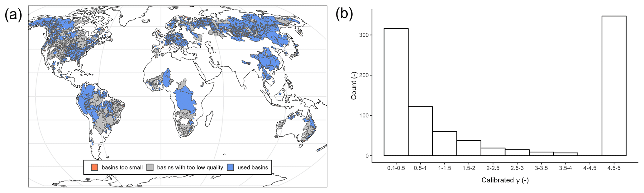
Figure 1(a) Map of calibrated basins, highlighting basins not used for regionalization due to insufficient model performance or inadequate basin size and (b) the histogram of the calibrated γ values for all basins used, showing a cluster of parameter values at the parameter bounds.
2.3 Basin descriptors
This study uses basin descriptors as predictors to drive regression-based or distance-based regionalization approaches. These basin descriptors are based on data used within the model simulation (as they are globally available). They are aggregated to basin values using a simple mean method to have the same spatial resolution as the calibrated model parameter. Thus, in the case of nested basins, the inter-basin area is used to define the basin descriptors. The selection of the predictors, i.e., basin descriptors that support the estimation of γ, is crucial for regionalization methods (Arsenault and Brissette, 2014). Typically, this selection aims to obtain the most information with the least number of predictors to (1) improve the model quality and (2) limit over-parametrization. In this study, we use 12 basin descriptors to develop regionalization methods; 9 of these descriptors are physiographic, while the remaining 3 are climatic (see Table 1). Most descriptors are not correlated (see Appendix C); i.e., we minimize redundant information (Wagener et al., 2004).
A descriptor subset is selected based on correlation analysis between basin descriptors and the calibrated γ value and entropy assessment. Pearson's correlation coefficient detects linear correlation, and Spearman's rho and Kendall's tau detect a non-linear correlation. Shannon entropy (Shannon, 1948) measures the information gain of the predictors explaining the calibrated γ value. The higher the information gain, the more valuable the basin descriptor is for explaining the variation in the calibrated γ value. The analysis directly evaluates the relationship between the calibrated parameter and the basin descriptors, as WaterGAP3 uses only one calibration parameter with a clear global optimum within the parameter space. An alternative would be to use flow characteristics to define the basis for regionalization (e.g., Pagliero et al., 2019). We decided to use the calibrated parameter instead of flow characteristics as it does not need any further assumption on which flow characteristics determine the model's parameter.
Statistical information of the evaluated basin descriptors and the corresponding correlation coefficients and information gain are listed in Table 1. The basin descriptors demonstrate a considerable degree of variability; e.g., the basin size ranges from 5000 to 3 112 480 km2 with a median of 13 796 km2. The mean temperature varies from −19 to 29 °C, and the sum of precipitation ranges from 213 to 5716 mm. Although there is a high degree of variability in the analyzed basin descriptors, the basin descriptors exhibit low correlation coefficients with the calibrated values. For example, the permafrost coverage shows the strongest Pearson correlation of −0.37 (and −0.50 for Spearman's rho). The information gain indicates the same results as the correlation analysis; i.e., the information gain is generally relatively low, and descriptors with a higher correlation tend to have a higher information gain. For example, the mean temperature exhibits the maximal information gain of 17.6 % and has the second-highest correlation coefficient, with a Pearson correlation of 0.34.
Table 1Basin descriptors – statistical information, correlation, and entropy assessment. Selected physiographic and climatic basin descriptors are written in bold.
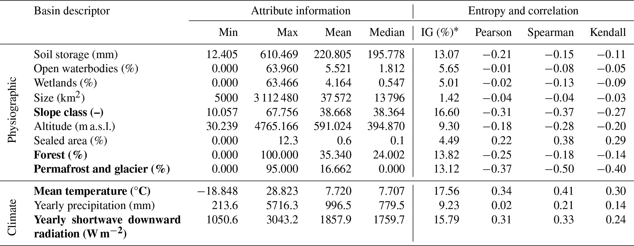
∗ Information gain is given in percentage of total information content in γ, after Shannon (1948).
In contrast to the findings of Wagener and Wheater (2006), the correlation coefficients between the basin descriptors and the calibrated values are relatively low, indicating a weak relationship. One potential explanation for this discrepancy is that Wagener and Wheater (2006) used a smaller number of basins in southeast England, with limited versatility (e.g., regarding climate and seasonality) compared to the 933 worldwide basins used in this study. Studies using a large number of basins likely tend to find a lower correlation between catchment attributes and model parameters (Merz and Blöschl, 2004). Moreover, the clustered calibrated γ values at the bounds of the valid parameter space may disturb the results of this analysis. As the calibrated value masks the effect of multiple sources of errors, such as uncertainty in the input data, model structure, or varying hydrological processes, finding a meaningful relationship between catchment characteristics and calibrated values is challenging.
Because the basis for the descriptor selection seems uncertain, given the low correlation and the named constraints, we additionally run the regionalization methods with all descriptors to evaluate the descriptor selection. Further on, to ascertain the advantage of integrating climatic descriptors, we run the regionalization methods using either physiographic or climatic descriptors. In total, we used four groups of basin descriptors to implement the regionalization methods:
-
“cl” – all 3 climatic descriptors;
-
“p” – all 9 physiographic descriptors;
-
“p+cl” – all 12 descriptors; and
-
“subset” – 2 correlated climatic descriptors (mean temperature, annual shortwave radiation) and 3 correlated physiographic descriptors (slope class, forest percentage, permafrost percentage).
2.4 Regionalization methods
In our study, we test several traditional and machine-learning-based regionalization methods against each other and against a defined benchmark to beat to find suitable regionalization methods for WaterGAP3. At the global scale, regionalization is particularly challenging due to (1) the lack of high-quality data, (2) the diversity of dominant hydrological processes in basins, and (3) the high computational demands of the models. Therefore, a robust regionalization method that applies to a wide variety of basins and is not computationally demanding should be selected for global application.
We test three common traditional approaches and two machine-learning-based approaches using the concepts of spatial proximity, physical similarity, and regression-based methods. As WaterGAP3's model calibration is very rigid and has only one parameter, it is not feasible to implement and test regionalization methods that incorporate regionalization into the calibration process, such as transfer functions. In addition, we avoid high computational demands, as all evaluated methods are applicable after the calibration, i.e., without running the model.
As the calibration of WaterGAP3 results in a parameter distribution with a cluster of parameter values at the parameter bounds, we implement a so-called “tuning” to introduce information about the parameter space into regionalization. In detail, we apply a simple threshold-based approach to shift the regionalized parameter values to the extremes, i.e., and The thresholds γ1 and γ2 are defined by applying the k-means algorithm with three centers to the calibrated parameter values. This clustering results in three clusters: one for low, one for medium, and one for high γ values. Subsequently, γ1 refers to the highest γ value of the low cluster, and γ2 refers to the lowest γ value of a high cluster.
To evaluate the regionalization methods, we implement an ensemble of split-sample tests. Specifically, we randomly split the basins into 50 % gauged (for training) and 50 % pseudo-ungauged (for testing). The split has a relatively high percentage of pseudo-ungauged basins, accounting for many missing gauges worldwide and for the high importance of generalizability. We fit the methods and apply them to the training and testing data sets. The split-sample test is repeated 100 times by randomly splitting the basins to account for sampling effects.
As there is only one calibration parameter, γ, this parameter has a global optimum per basin. Consequently, the quality of training and testing is directly assessed by the deviation between the regionalized and the calibrated value for γ. The closer the regionalized values are to the calibrated ones, the more accurate the prediction. We assess the prediction accuracy by the logarithmic version of the mean absolute error (logMAE) shown in Eq. (3) to account for the decreasing sensitivity of γ for higher values (see Appendix B). The lower the logMAE, the better the prediction; a zero value in logMAE expresses no error. The regionalization method is robust if the prediction accuracy is similar in training and testing. A generally good performance, i.e., small logMAE values, indicates that the regionalization method suits WaterGAP3. The comparison of γ values enables the application of a wide range of regionalization methods and sets of descriptors, as no computationally intensive model simulation is required. However, it assumes that deviations in γ lead, in turn, to deviations in discharge, which is only partially true because of varying parameter sensitivity in basins (e.g., Kupzig et al., 2023). To validate that the logMAE is a sufficient approximator of the regionalization performance in WaterGAP3, we use one representative split sample from the ensemble to compare the accuracies in simulated discharge for different regionalization methods.
where n is the number of basins in the corresponding sample, γx,i is the calibrated value of γ for the ith basin, and γy,i is the estimated value of γ for the ith basin. We applied a Box–Cox-type transformation with λ1=0 and λ2=1 (Box and Cox, 1964) to calculate the logMAE, avoiding negatively transformed values.
2.4.1 Regression-based methods
The traditionally used regionalization approach in WaterGAP3 is a regression-based MLR. As the benchmark to beat, we use the regionalization approach from WaterGAP v2.2d defined in Müller Schmied et al. (2021). We consider it a suitable benchmark to beat given that WaterGAP2 has a model structure and calibration process that is very similar to WaterGAP3. The main difference between these models is that WaterGAP2 simulates at a 0.5° spatial resolution. The benchmark to beat consists of “a multiple linear regression approach that relates the natural logarithm of γ to basin descriptors (mean annual temperature, mean available soil water capacity, fraction of local and global lakes and wetlands, mean basin land surface slope, fraction of permanent snow and ice, aquifer-related groundwater recharge factor)” (Müller Schmied et al., 2021). We fit this regression model to our data and define the quality of this approach as the benchmark to beat. Moreover, we test an independent MLR approach without using the logarithmical scaling of γ and using the above-defined sets of basin descriptors. For MLR and the benchmark to beat, we use the lm() function of the R package stats (R Core Team, 2020). After applying the regression model, we adjust the estimated parameter values to ensure that the estimated values range between 0.1 and 5.
Furthermore, a machine-learning-based method, random forest (RF), is tested for regionalization as an alternative to MLR. Here, we implement the random forest algorithm with the randomForest() function from the R package randomForest (Liam and Wiener, 2002), which is based on Breimann (2001). The algorithm uses an ensemble of decision trees, making the decision human-like. It is relatively robust because it incorporates random effects into the training process. To implement this randomness, we define the algorithm as one that can choose between two randomly selected predictors at each node, using an ensemble of 200 trees.
2.4.2 Physical similarity
As the traditional physical similarity approach, we use similarity indices (called SIs in the following), applying the methodology proposed by Beck et al. (2016). The SIs (see Eq. 4) are derived using the defined basin descriptors sets, and the parameter of the most similar basin is transferred to the pseudo-ungauged basin. Additionally, we use an ensemble of basins to control whether an ensemble-based approach leads to more robust results. The optimal number of donor basins may vary between research regions and hydrological models (Guo et al., 2020). Here, we use 10 donor catchments (noted by ensemble) based on Beck et al. (2016) and McIntyre et al. (2005). Further, we apply a simple mean method for the ensemble-based prediction to aggregate the ensemble of γ values into one predicted parameter value.
where Si,j is the similarity index between basin i and basin j, Zp,j is the basin descriptor p for basin j, IQRp is the interquartile range for basin descriptor p among all (gauged) basins, and n is the number of all basin descriptors used.
As an alternative machine-learning-based approach, we apply a simple k-means algorithm. We selected the k-means algorithm because it is one of the most widely used clustering algorithms (Tongal and Sivakumar, 2017). It is easy to understand and use. The algorithm kmeans() is implemented in the R base package stats. It aims to maximize variation between groups and minimize variation within groups. The number of clusters to use is determined by multiple indices calculated with the R package NbClust (Charrad et al., 2014). For all 933 basins and the defined sets of basin descriptors, most indices defined 3 as the optimal number of clusters. Accordingly, we use three clusters to generate the groups of basins. As different scales of the predictor values can affect the clustering, a rescaling with min–max normalization (see Eq. 5) is performed on the training set and applied to the testing set. After the grouping, the mean γ value is assigned as a representative calibrated value to the corresponding basin group. To estimate the corresponding group for a pseudo-ungauged basin, the k-nearest neighbour (knn) algorithm is used, and the representative γ value of the group is assigned to the pseudo-ungauged basin. This algorithm is implemented by the knn() function of the R package class (Venables and Ripley, 2002). Since the k-means method is less flexible than SI, we implement a highly flexible version, using the knn algorithm directly to define the donor basin most similar to each ungauged basin. Using the knn algorithm directly, we test how beneficial it is to create groups of similar basins using the kmeans algorithm and regionalize the parameter with a representative mean value.
where is the normalized basin descriptor p for basin j, Zp,j is the basin descriptor p for the basin j, and m is the number of (gauged) basins.
2.4.3 Spatial proximity
The spatial proximity approach is one of the easiest to use to regionalize parameter values. However, it is also often criticized because nearby basins do not necessarily have the same hydrological behavior (Wagener et al., 2004). Furthermore, its performance depends on the density of the network of gauged basins (Lebecherel et al., 2016). The dependency on network density is particularly challenging for global applications where large parts of the world are ungauged (e.g., northern Africa). Nevertheless, the approach has been successfully applied in other studies (e.g., Oudin et al., 2008; Qi et al., 2020), even globally (Widén-Nilsson et al., 2007). Here, we take the distance between the centroids of the basins as the reference for the spatial distance between basins, as done by others (Oudin et al., 2008; Merz and Blöschl, 2004). We use the abbreviation SP in the text below to refer to the spatial proximity approach. Figure 2 provides an overview of the applied regionalization methods and information used for the experimental setup.
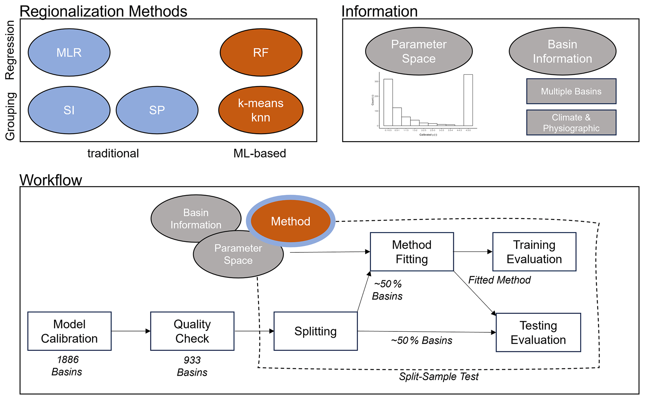
Figure 2Experimental setup of the study – regionalization methods, modifications and information used, and the general workflow (MLR is multiple linear regression, SI is similarity indices, SP is spatial proximity, and RF is random forest).
3.1 Evaluating the effect of tuning
First, the impact of the tuning approach on the regionalization approaches is evaluated. Therefore, Fig. 3 depicts the differences in logMAE between the standard and tuned approaches in testing, i.e., using the pseudo-ungauged basins. A positive difference in logMAE indicates an increase in accuracy, whereas a negative difference indicates a decrease in accuracy due to the tuning.
Using the tuning thresholds of about 1.1 and 3.4 for γ1 and γ2, respectively, enhances the predictive accuracy for kmeans, MLR, RF, and the ensemble approach of SI. The most remarkable improvement for kmeans, RF, and the SI ensemble is achieved when all physiographic descriptors are used as input (mean improvement of 0.077, 0.058, and 0.071, respectively). MLR shows the most significant improvement when using all available descriptors (mean improvement of 0.038). In contrast, the tuning decreases the performance for knn, SI, and SP, with a mean degradation between −0.02 and −0.05. Unlike the enhanced regionalization techniques, these methods transfer single-basin information to ungauged regions. Thus, the tuning disturbs the use of single-basin information yet simultaneously enhances the performance of methods that transfer multi-basin information. The disturbance or improvement is probably related to the capability of the methods representing the clustering of parameter values at the extremes: while the multi-basin information transfer implies a smoothing and thus suffers from a lack of representation of the extremes, the single-basin information transfer exhibits no such smoothing.
The exception to the above-defined rule is the benchmark-to-beat approach. The benchmark to beat is the only approach that uses logarithmic scaled γ values when fitting the model. This logarithmic transformation leads to an increase in estimating small values. Thus, when the benchmark to beat is tuned, more basins with higher calibrated γ values receive low estimates. The tuning intensifies this effect, leading to a decrease in the accuracy of the logMAE from the standard to the tuned version. Thus, for models using logarithmical transformed γ values, the defined thresholds for the tuning are not appropriate.
Applying knowledge of the optimal parameter space enhances the quality of regionalization for methods transferring multi-basin information in cases where the tuning thresholds are appropriate. This positive effect is not surprising, as incorporating a priori information about parameter distribution strengthens parameter estimation (e.g., described in Tang et al., 2016 using the Bayes theorem). However, for single-basin transfer, which already represents the parameter space well, i.e., the clustering of γ at the extremes, the tuning disturbs the performance. This indicates that such tuning needs to be cautiously introduced as there is the risk of decreasing the accuracy of regionalization.
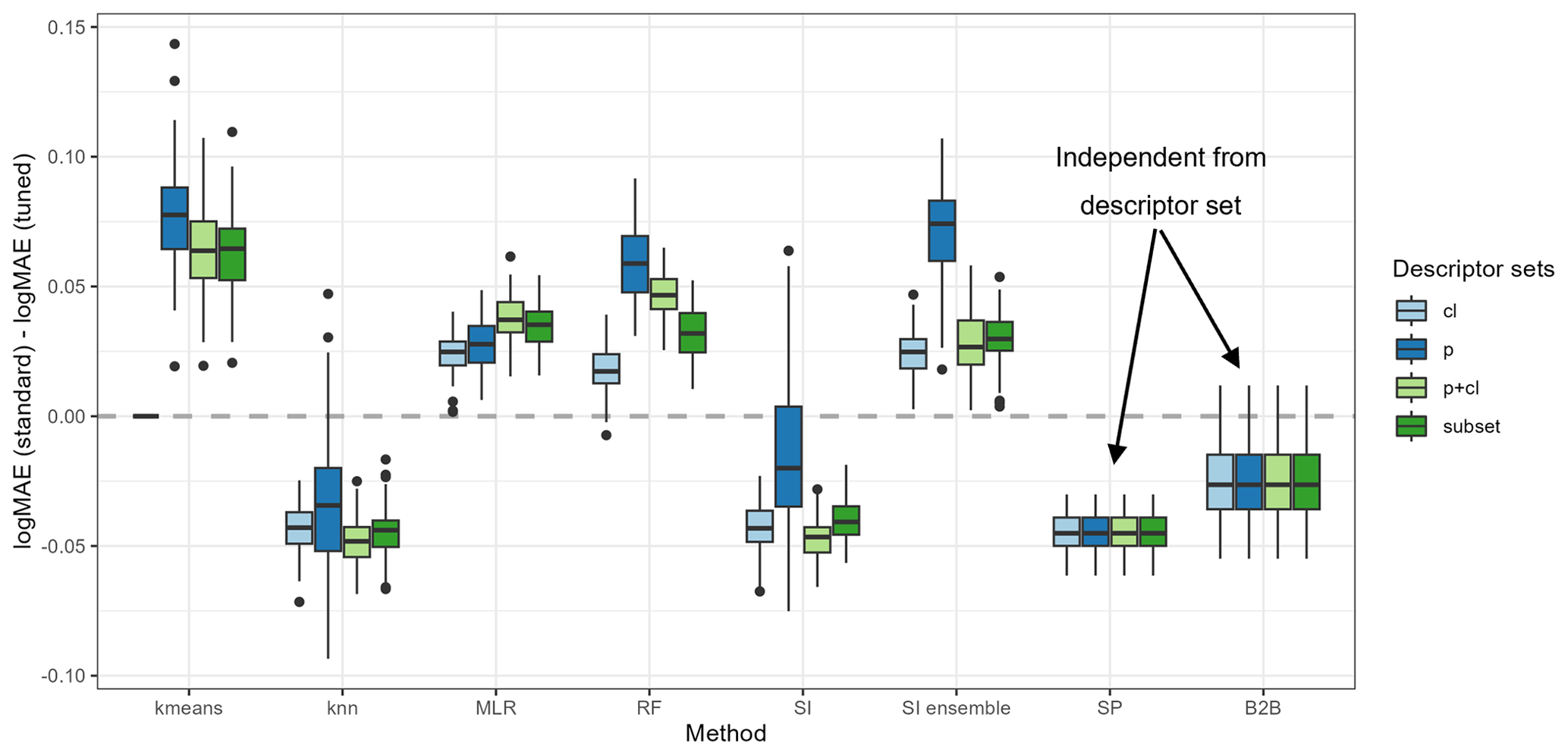
Figure 3Changes in performance between standard and tuned versions for all applied regionalization approaches. Positive values indicate an improvement related to the tuning.
3.2 Evaluating descriptor subsets and algorithm selection
Different descriptor sets yield different performance in regionalizing γ. Table 2 shows the median of all logMAE values for the testing. For a complete overview of the results of the split-sample test ensemble, see Appendix D. Evaluating Table 2 reveals that the selected subset or all descriptors consistently yield the best performance across all regionalization methods. In both variants of the ensemble approach of SI, in the tuned version of the no-ensemble approach of SI, and in the standard version of RF, the selected subset yields the best results. For all other methods, using all descriptors yields the best results. Hence, all methods perform best when combining climatic and physiographic descriptors. This benefit of using climatic and physiographic descriptors is consistent with others that often apply a combination of climatic and physiographic descriptors, achieving optimal regionalization results (e.g., Oudin et al., 2008; Reichl et al., 2009).
The machine-learning-based approaches seem to benefit most when using more information, displaying an improvement for all methods (knn, kmeans, and RF) and both variants (standard and tuned) ranging from cl, p, and subset to p+cl. This is not surprising as machine learning was developed to deal with big data sets. The traditional methods of MLR and SI do not exhibit such a distinct pattern. The (weakly) correlated subset of climatic and physiographic descriptors yields the best results for SI. As utilizing all descriptors decreases the performance slightly, the results indicate that uncorrelated descriptors may disturb the performance of this approach. For MLR, the meaning of physiographic information is highest, resulting in the best (p+cl) and second-best (p) results. The disparate performance of the regionalization methods when using different descriptor sets indicates that different methods use descriptor sets with varying efficiency. It also emphasizes that the selection of descriptors impacts the regionalization method's results, as noted by others (Arsenault and Brissette, 2014). Consequently, the analysis performed above that defines a descriptor subset lacks universal validity, as methods exist where the defined subset is outperformed. Instead, the validity of this approach is most closely aligned with the SI approaches.
Although the algorithms kmeans and knn are similar, they yield considerably different performance in Table 2. As knn shows a logMAE of 0.432 at best, the kmeans algorithm performs poorly, resulting in the best logMAE of 0.472. This indicates that applying the k-means clustering algorithm to transfer-averaged parameters is inappropriate for WaterGAP3. This may be attributed to the reduced flexibility of the approach, which entails estimating only three γ values due to the optimal, although limited, number of centers. The ensemble SI approach consistently outperforms the no-ensemble SI approach in almost all variants. The positive effect of an ensemble approach for SI has already been noted (Oudin et al., 2008). Therefore, it is recommended that the number of donor basins derived from the literature be adopted in future applications as optimal for WaterGAP3, likely resulting in higher performance.
Table 2Median logMAE of 100 split samples for pseudo-ungauged basins, i.e., in testing, for all regionalization methods applying four sets of descriptors for (a) the standard version and (b) the tuned version. The bold numbers indicate better performance than the benchmark to beat. Thicker edges mark best-performing variants, which are chosen for further analysis. Gray-shaded cells indicate worst-performing variants, which were taken to validate the assumption that lower logMAE values result in lower KGE values.
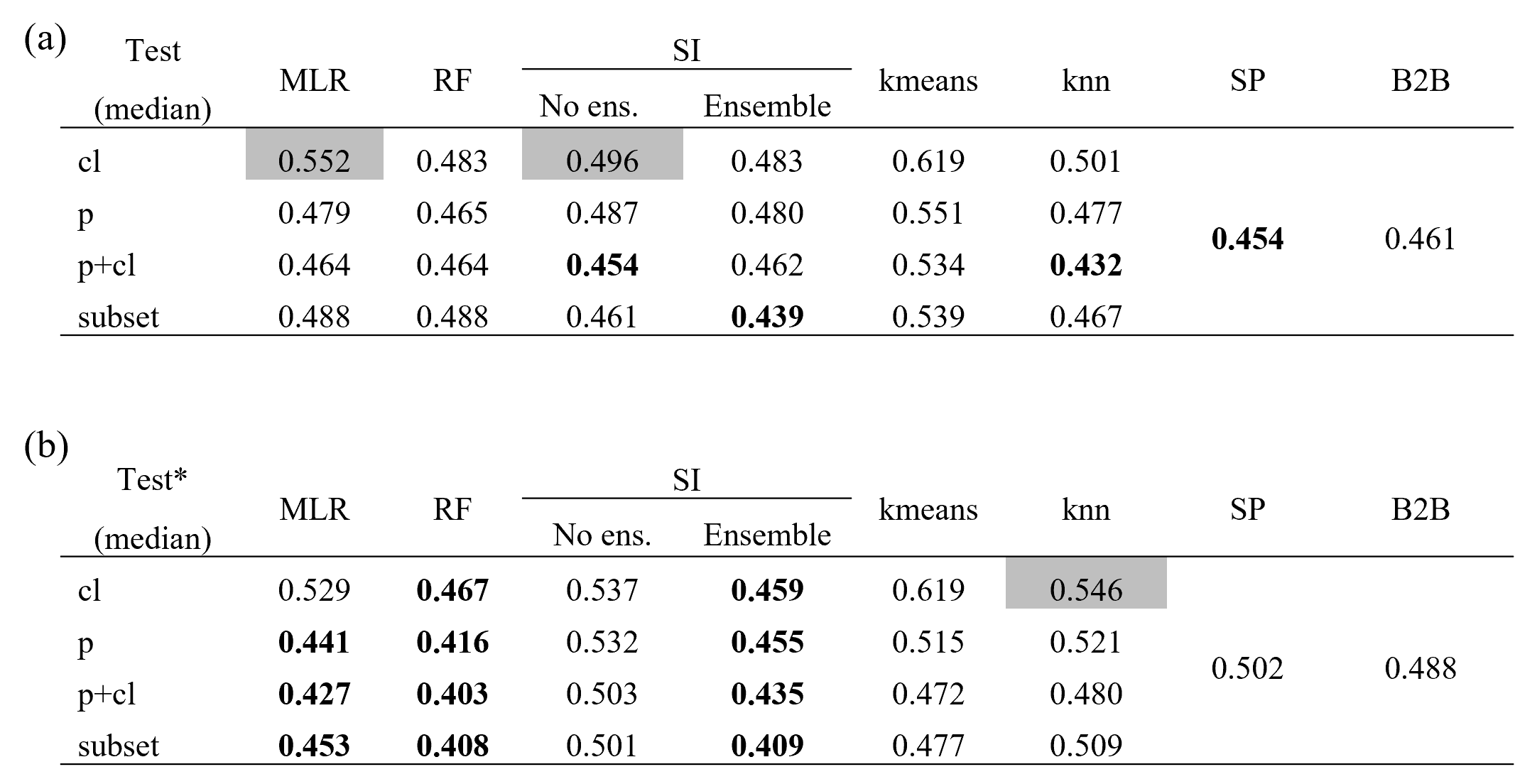
Only a few regionalization methods outperform the benchmark to beat. The best descriptor sets of the tuned MLR, RF, and SI ensemble approach have a logMAE of 0.427, 0.403, and 0.409, respectively. The standard version of knn (p+cl) and SP yield 0.432 and 0.454 in logMAE, respectively. Additionally, two variants of the standard SI approaches outperform the benchmark to beat yet exhibit inferior results compared to the selected tuned approach. All other regionalization methods show higher logMAE values than the benchmark to beat. These methods are considered insufficient in terms of performance to regionalize γ in WaterGAP3. As the benchmark to beat outperforms all kmeans approach variants, it is deemed unsuitable for regionalizing γ for WaterGAP3 and, therefore, is excluded from further analysis.
The good performance of SP on a global scale is surprising as the distances between basins are potentially long, and hydrological processes may strongly vary. It is probably beneficial for the SP approach that γ comprises all kinds of errors, e.g., spatially localized errors in global forcing products (e.g., Beck et al., 2017, reported errors for arid regions in the precipitation product), or inaccurately represented processes for larger regions. Thus, the estimation of γ might be appropriate not because of the same hydrological behavior but due to the same kind of errors.
The RF approach is remarkable, as it shows a massive loss in performance from training to testing (see Appendix D). In detail, the logMAE in testing is about twice the logMAE in training. In comparison, other methods show values of logMAE in testing ranging from 95.6 % to 101.4 % of logMAE in training. This performance loss indicates that RF is not a robust regionalization method for WaterGAP3. Other studies that reported the good performance of RF for regionalization have not investigated the stability of the performance from training to testing (Golian et al., 2021; Wu et al., 2023). Likely, the mathematical problem of predicting the calibrated parameter for WaterGAP3, with all its challenges (e.g., tailored parameter space, clustered calibrated parameter, and incorporation of many sources of errors), cannot be adequately solved by RF. Thus, although RF is known to be especially robust among other machine-learning-based techniques, it shows symptoms of over-parameterization. This indicates that the algorithm is too flexible and adjusts to noise in the data, missing the underlying systematic. This lack of robustness is particularly disadvantageous since, for WaterGAP3, regionalization is applied globally, requiring regionalizing large parts of the world. In consequence, the RF approach is left out from further analysis and is defined as not suitable to regionalize γ for WaterGAP3.
For the tuned MLR approach and the knn approach, the best-performing and, therefore, selected variant employs all 12 descriptors. This number of predictors for a regionalization method is among the highest found in the literature (e.g., McIntyre et al., 2005, used 3 predictors; Beck et al., 2016, used 8 predictors; and Chaney et al., 2016, used 13 predictors). In general, it is advisable to limit the number of degrees of freedom in a model to reduce the risk of over-parametrization, thus increasing the probability of generalizability (Seibert et al., 2019). As both model variants exhibit stable model performance during training and testing (see Table D1), using a high proportion of the basins for testing, i.e., 50 %, we consider the two variants robust despite the relatively high number of predictors used. Therefore, we consider them appropriate for further model evaluation.
Nevertheless, the chosen basin descriptors for knn and tuned MLR could be enhanced in future studies. As the descriptor set p+cl was initially considered a control group to determine the suitability of the selected subset, it is not optimal. To indicate potential enhancements regarding the descriptor set for both methods, we calculated a simple permutation-based feature importance score (see Breiman, 2001) by randomly shuffling each predictor within the testing data set and quantifying the loss in logMAE relative to the logMAE of the original testing data set. The higher the loss, the more critical the shuffled predictor for the regionalization method. The resulting feature importance scores are presented in Appendix E, indicating that for the tuned MLR, the subset of (weakly) correlated descriptors should be extended by including waterbody information. For the knn approach, the calculated feature importance scores indicate that it should be extended by including information about the soil storage.
3.3 Performance of selected algorithm in pseudo-ungauged basins
To avoid the high risk of sampling effects when applying the split-sample test, we conduct an ensemble of 100 split-sample tests, analyzing the median of logMAE between regionalized and calibrated values as an indicator for performance. Directly using the differences in regionalized and calibrated values is only meaningful when the calibrated value represents the global optimum. This is often not the case, e.g., due to equifinality, the performance of regionalization methods is usually assessed by the accuracy of simulated discharge (e.g., Samaniego et al., 2010; Arsenault and Brissette, 2014). Because WaterGAP3 requires computationally intensive simulations, running WaterGAP3 for all 100 split-sample tests for the selected methods is not feasible. Therefore, we select a single representative split sample to assess the quality of representing the discharge in the pseudo-ungauged basins using regionalized γ values. The representative split sample leads to comparable logMAE values to the corresponding median of the ensemble for all regionalization methods. For the evaluation, WaterGAP3 was run for the same period used in calibration (from 1979 to 2016), with the first year simulated 10 times to allow for model warmup. Using this period ensures the availability of sufficient data for the evaluation (see Sect. 2.2). Furthermore, the differences between the monthly simulated and observed discharge are assessed using the KGE.
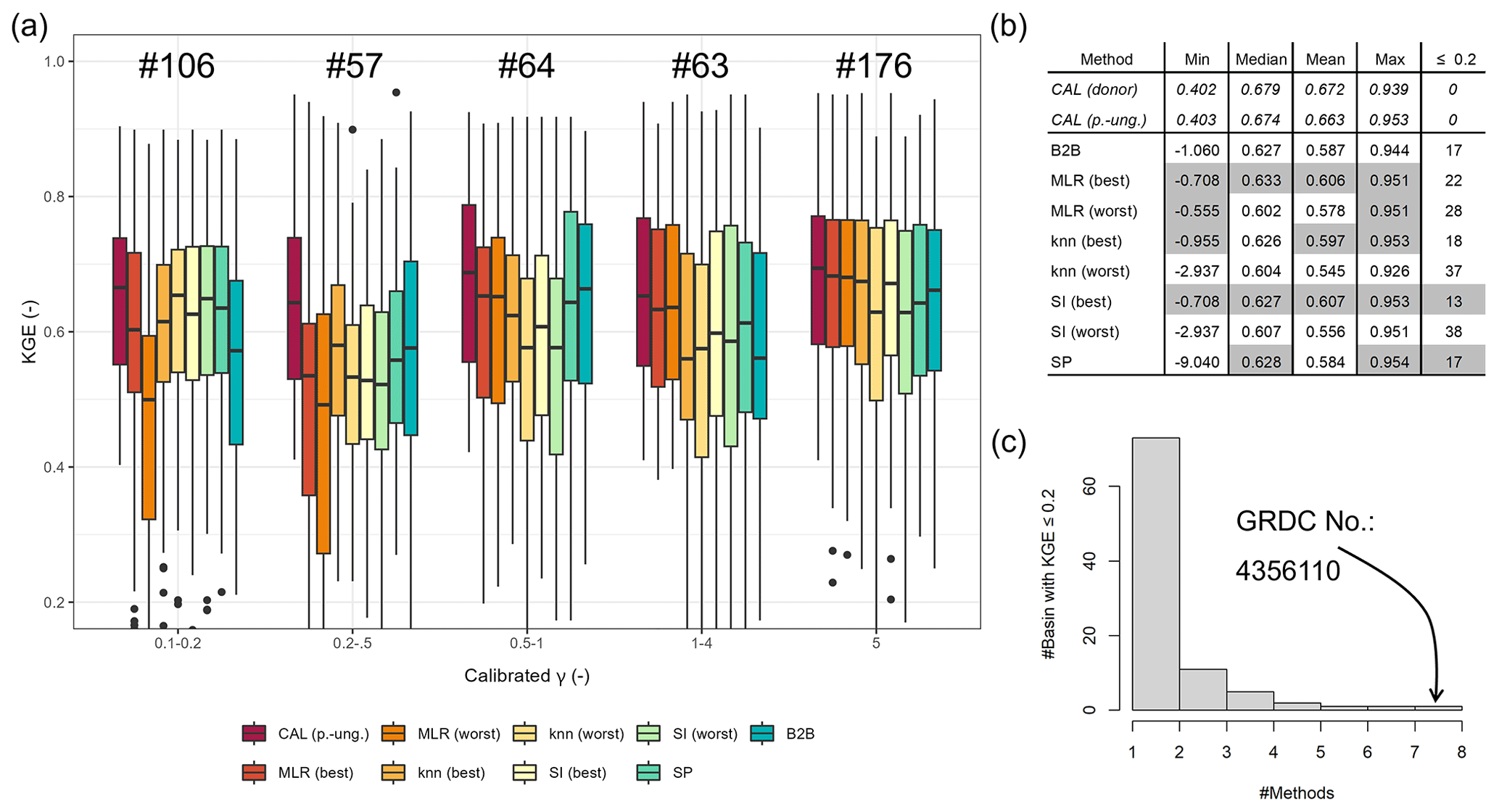
Figure 4(a) KGE values of pseudo-ungauged basins from the split-sample test grouped by the range of calibrated γ values. (b) Selected metrics of KGE values from the pseudo-ungauged basins (performance better than or equal to the benchmark to beat is highlighted in gray). (c) Histogram of the number of pseudo-ungauged basins with a KGE below 0.2 and the corresponding number of methods exhibiting this performance loss.
To evaluate the KGE, we select the best-performing methods that outperform the benchmark to beat: tuned MLR p+cl, knn p+cl, tuned SI ensemble subset, and SP (see Table 2). For the sake of simplicity, we further mark them with “best”. Additionally, we select three poorly performing variants to validate the assumption that methods resulting in higher logMAE values tend to result in lower KGE values, i.e., lower accuracy of simulated discharge. These methods are tuned SI cl (logMAE = 0.537), tuned knn cl (logMAE = 0.546), and MLR cl (logMAE = 0.552). Further, we denote these methods “worst”. Applying the selected methods and the benchmark-to-beat method results in eight estimates of γ for the pseudo-ungauged basins, whose performance is further evaluated in terms of simulated discharge accuracy.
Figure 4a shows the resulting KGE values for the evaluated regionalization methods and the calibrated version as grouped boxplots for different ranges of calibrated γ. The methods show different performance for different γ ranges, indicating their strengths and weaknesses. For the smallest γ range, 0.1–0.2, the selected methods that perform well during the split-sample test outperform the benchmark to beat. The better result for minimal γ ranges is probably partially related to the advantage of the tuning, which leads to more predictions of 0.1 within the regionalization. The benchmark to beat shows the best performance for γ values between 0.2 and 0.5. The good performance for basins with calibrated γ values between 0.2 and 0.5 is probably related to the benefit of using the logarithmical version of γ in the benchmark to beat, leading to more estimates of smaller values. However, this affects only 12 % of the basins, as calibrated values between 0.2 and 0.5 are not frequently present in the calibration result. Generally, the differences in KGE appear higher for smaller γ values, probably due to the decreasing parameter sensitivity with higher values (see Appendix B).
Given the variability in the performance of the regionalization methods across the depicted γ ranges, it is challenging to identify an overall-best regionalization method using Fig. 4a. Therefore, we compare the various metrics of the KGE values depicted in Fig. 4b. The analyzed metrics are the minimum, maximum, mean, and median. Further, we count the number of poorly performing basins, defined as basins with a KGE below 0.2. In Fig. 4b, metrics that exceed the benchmark to beat are gray shaded. Comparing the KGE metrics in Fig. 4b reveals that the methods showing higher logMAE values in our split-sampling test ensemble also show lower performance in simulating discharge. For example, all mean (and median) KGE values of the worst methods are below the mean KGE of 0.587 from the benchmark to beat, ranging from 0.545 to 0.578. This indicates that the logMAE used between regionalized and calibrated values is a valid tool for a preliminary selection of adequate methods for the regionalization of WaterGAP3. However, for a more comprehensive analysis, we recommend additionally analyzing the accuracy of simulated discharge, as the logMAE of calibrated and regionalized parameter values simplifies the inherent complexity between model parameters and model performance.
Moreover, SI (best) outperforms the benchmark to beat in all listed metrics, reducing poorly performing basins and enhancing well-performing basins. MLR (best) performs very similarly to SI (best), yet it shows a higher number of basins with KGE values below 0.2. In comparison to the benchmark to beat, it outperforms four out of five criteria. The remaining well-performing methods, SP and knn (best), demonstrate superior or equal performance to the benchmark to beat in three out of five criteria. SP results in an equal number of poorly performing basins, and the minimal KGE value is lower than for the benchmark to beat. The knn (best) approach has a slightly worse median KGE, i.e., −0.001, and one additional basin shows a KGE below 0.2.
As SI (best) outperforms the benchmark to beat in all metrics, we conduct a statistical test to ascertain whether there is a statistically significant difference in KGE results between the methods. To this end, we use a one-sided paired Wilcoxon rank-sum test to test the null hypothesis of whether the KGE differs significantly in central tendency. A significance level of 0.05 and an adjusted p value are applied to correct for multiple comparisons (using the correction from Benjamini and Hochberg, 1995). The results (see Fig. F1c) demonstrate that SI (best) outperforms all the worst methods and the benchmark to beat. However, the null hypothesis for SP and the best options of knn and MLR cannot be rejected. Consequently, rather than identifying a single alternative to the benchmark to beat, we have identified four.
Notably, all regionalization methods lead to poorly performing basins, as evidenced by the range of basins with a KGE below 0.2, varying from 13 to 37. In Fig. 4c, we examine whether there are basins that all methods cannot regionalize, thereby indicating a general insufficiency of the regionalization methods for these basins. The histogram indicates that most poorly performing basins belong to a single regionalization method. The high number of basins that cannot be estimated well by a single regionalization method illustrates the diverse shortcomings of the methods. A single basin shows poor performance across all methods. This is a basin of the river El Platanito in Mexico. The calibrated γ value is about 1.5, and the corresponding KGE value in calibration is 0.466. This basin appears to be highly sensitive to γ, with an inaccuracy in the estimated γ having a significant impact on the accuracy of river discharge. For example, the benchmark to beat estimates γ to 1.0, which is close to the calibrated value of 1.5. However, the KGE value of the simulated discharge using the benchmark to beat is −0.158 due to a high overestimation of the variation and mean of the discharge. This high sensitivity seems remarkable and is likely attributable to the absence of waterbodies and snow, supporting a potentially high impact of γ on the model simulation (Kupzig et al., 2023) in conjunction with a relatively small basin size (ca. 6600 km2).
Model evaluation is at least partially subjective (Ritter and Muñoz-Carpena, 2013), and the choice of evaluation criteria represents a source of uncertainty in model performance evaluation (Onyutha, 2024). Furthermore, the choice should reflect the intended model use (Janssen and Heuberger, 1995). As GHMs are often applied to evaluate monthly simulated discharge (e.g., Herbert and Döll, 2023; Jones et al., 2024; Tilahun et al., 2024), we assess the model performance using monthly data. Moreover, GHMs are generalists rather than expert models; thus, the model evaluation should encompass a range of aspects related to streamflow to obtain an overall metric. Therefore, we applied the monthly KGE, which comprises information about the streamflow's variability, bias, and timing. As we use monthly values, we expect that outliers, i.e., single flood events, are less influential than in daily data sets. Consequently, we expect the disadvantage in the KGE exhibiting sampling uncertainty to be less significant (see Clark et al., 2021).
Nevertheless, to reduce the risk that disadvantages of the evaluation criteria influence the model evaluation, we conducted an additional model evaluation using a modified version of the Nash–Sutcliff efficiency (NSE; Nash and Sutcliff, 1970). This modified NSE uses absolute differences instead of squared terms, leading to a metric that is especially suitable as an overall measure (Krause et al., 2005). The results of the analysis are in Appendix F. The high boxplot similarity between the modified NSE and the KGE confirms that the monthly KGE represents the overall monthly model quality. Moreover, the statistical metrics of the modified NSE indicate that MLR (best), in particular, outperforms the benchmark to beat. Applying the one-sided paired Wilcoxon rank-sum test on the modified NSE reveals that knn (best), SI (best), and the benchmark to beat deliver no statistically significant differences in the central tendency from the well-performing MLR (best). These differences in results illustrate that the choice of evaluation criteria can significantly impact the experimental outcome. Moreover, it underpins the usefulness of evaluating ensemble approaches to account for this inherent uncertainty.
3.4 Impacts on runoff simulations
To evaluate the impact of runoff simulations, we apply an ensemble of regionalization methods generating γ estimates for the worldwide ungauged regions. Within the ensemble, we use the four methods, SI (best), knn (best), MLR (best), and SP, that (1) outperform the benchmark to beat regarding the logMAE of regionalized and calibrated values and (2) perform similarly to each other and better than the benchmark to beat in KGE for monthly discharge. Additionally, we use the benchmark to beat as the fifth member of our regionalization method ensemble, as it shows no significantly weaker performance than the well-performing MLR (best) for the modified NSE. The entire set of 933 gauged basins is used for regionalizing γ, resulting in 5 distinct worldwide distributions of γ. The spatially distributed standard deviation of the regionalized values is shown in Fig. 5.
In particular, the southern parts of South America, the northern and southern parts of North America, and central Asia reveal differences in γ across the ensemble of regionalization methods (see Fig. 5). In Europe, the highest differences in regionalized values are observed in Italy, Great Britain, and northern Portugal. In Oceania, the highest values in standard deviation of γ are in Tasmania, New Zealand, and the southwest of Australia's coast. In contrast, a minor variation in γ is apparent in northern Africa, most parts of Australia, and east of the Dead Sea. Thus, the uncertainty associated with globally regionalizing γ seems to vary across different regions.
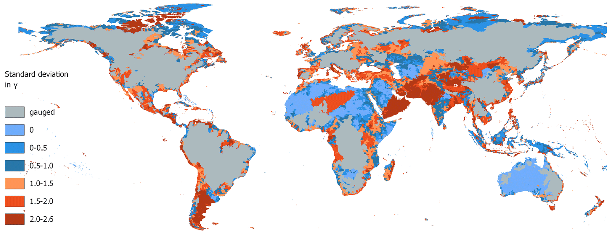
Figure 5Standard deviation in regionalized γ values using the best approaches of MLR (best), SI (best), SP, knn (best), and the benchmark to beat. Note that dry regions without discharge are set to zero.
An example of how these uncertainties in regionalized values propagate through the water system is presented in Fig. 6. This figure displays the coefficient of variation in the mean yearly discharge between 1980 and 2016 based on the five simulation runs. Moreover, we highlight the effect on rivers in ungauged regions by showing the resulting seasonal pattern, i.e., the simulated long-term mean of monthly river discharge for three exemplary rivers. These rivers are the Río Bravo in Mexico, the Tiber River in Italy, and the Tamar River in Tasmania. Each river is located in an ungauged region, where the standard deviation in γ is high (see Fig. 5).
Comparing Figs. 5 and 6 reveals that regions showing variability in γ tend to exhibit variation in mean yearly discharge. However, the impact of variation in γ on the simulated discharge appears to vary spatially. Some regions showing a high degree of variation in γ do not exhibit a correspondingly high degree of variation in discharge. For example, 45 % of all ungauged regions showing a low variation in discharge, i.e., the coefficient of variation is below 0.5, exhibit a standard deviation of more than 1 in γ. In contrast, about 89 % of the ungauged regions showing a higher discharge variation exhibit a standard deviation of more than 1 in γ. Thus, variation in γ does not necessarily lead to variation in river discharge, but it increases the likelihood that a region's discharge is affected. The spatially varying impact of γ is likely related to varying sensitivity regarding γ in the ungauged regions, which depends on numerous aspects, e.g., snow occurrence or waterbodies (see Kupzig et al., 2023).
About 11 % of the ungauged area exhibits variations in yearly river discharge exceeding 50 % of the mean. These regions are primarily in southern South America and central Asia. A further 62 % of the ungauged area exhibits variations in yearly river discharge between 10 % and 50 % of the mean. These regions are mainly located on the northern coast of Russia and in northern Canada, Indonesia, and Tasmania. Other areas, like most ungauged regions of Africa and Australia, show almost no impact; i.e., the variation in yearly discharge is less than 10 % of the mean. In northern Africa, one region exhibits higher values in the coefficients of variation. These values are attributable to minimal discharge values, resulting in comparatively high coefficients of variation in this region.
Considering the variation in the seasonality in the selected ungauged river systems (see Fig. 6b–d), the temporal impact of regionalization varies across the local landscape. For the Tamar River in Tasmania, as illustrated in Fig. 6d, the variation is higher at the start and end of the dry periods in October and November and in April and May, respectively. The spread in monthly mean discharge is about 0.7 to 1 m3 s−1 in these periods. The Tiber River in Italy and the Río Bravo in Mexico exhibit a similar pattern: using the regionalized γ values of SP leads to much higher discharge rates than other ensemble members, introducing broad uncertainty bands. For the Tiber River, this leads to seasonal estimates varying between 1.2 % (in January) and 11 % (in October) of the mean yearly sum. The Río Bravo shows variations in its seasonal pattern, with values ranging from 2.2 % (in February) to 6.8 % (in October) of the mean yearly sum. Thus, all rivers display a temporally varying impact. While the main variation in the discharge of the Río Bravo and the Tiber River is mainly attributed to the SP regionalization run, for the Tamar River, all regionalization runs contribute to the varying long-term monthly mean in discharge.
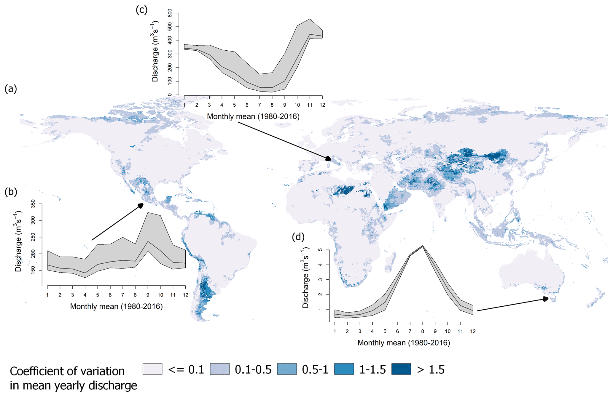
Figure 6(a) Global map of the coefficient of variation in mean yearly discharge for the applied regionalization methods. Resulting differences in the regionalization ensemble regarding the long-term mean of monthly discharge are depicted for (b) the Río Bravo in Mexico, (c) the Tiber River in Italy, and (d) the Tamar River in Tasmania. The gray-shaded area indicates the range of the long-term mean of monthly discharge, and the black line indicates the mean of all simulation runs.
To gain a deeper understanding of the local impact of regionalization on runoff simulations, we analyze the annual percentiles from 1980 to 2016 for Río Deseado in Argentina, Río Bravo, and Tamar River, displaying the mean percentile of all years (see Fig. 7a–c). As the Tiber River and Río Bravo display high similarities in the resulting patterns of percentiles, we demonstrate the impact by showing the percentiles from the Río Bravo. Additionally, we compare the relative differences in the mean for each percentile using eight ungauged river systems (see Fig. 7d), as was previously done by Gudmundsson et al. (2012) for nine GHMs. To calculate the relative difference, we subtract the mean annual percentile of a method from the corresponding mean annual percentile of the reference and divide the resulting difference by the mean annual percentile of the reference. Instead of using observed flow as a reference, we use the annual percentiles of our benchmark to beat. As river discharge is already spatially aggregated information, it is unnecessary to spatially aggregate grid cells to create results comparable to those of Gudmundsson et al. (2012), who used cell runoff. The evaluated river systems are the Río Chubut, Río Deseado, Río Negro, Río Bravo, Tamar River, Tiber River, Pescara River, and Ebro River.
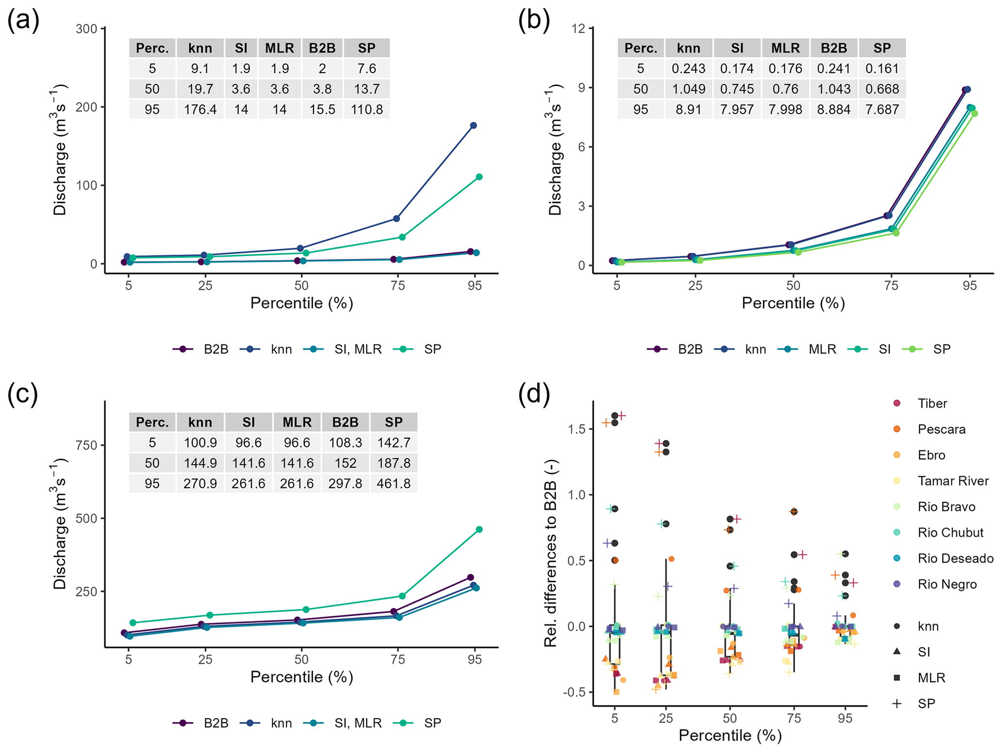
Figure 7Mean annual percentiles between 1980 and 2016 of simulated discharge using an ensemble of regionalization methods. The rivers are the (a) Río Deseado, (b) Tamar River, and (c) Río Bravo. In (d), the relative differences in mean annual percentiles from the benchmark to beat of eight ungauged river systems are presented. Negative values indicate smaller mean annual percentiles than the benchmark to beat. Note that all data points from Río Deseado for knn and SP are excluded as the values are above 2.0.
Fig. 7a shows that the Río Deseado is highly affected by uncertainties in simulated discharge due to the different regionalization methods; all segments of the percentiles show high variations where the absolute spread is increasing with increasing percentiles. For SP and knn (best), the discharge is highest, e.g., estimating a median discharge of 13.7 and 19.7 m3 s−1, respectively. For the other methods, the simulated discharge is low; e.g., SI and MLR result in an equal median discharge of 3.6 m3 s−1. The Tamar River in Fig. 7b also shows increasing absolute differences between the methods for higher percentiles, with the benchmark-to-beat approach leading to the highest discharge. For the Río Bravo, the absolute differences between the highest result of SP and the other methods remain almost constant until the 75th percentile. For the 95th percentile, the absolute differences increase rapidly from about 40 m3 s−1 (75th percentile) to nearly 200 m3 s−1 (95th percentile). The exemplary results of Río Deseado and Río Bravo indicate a potentially high degree of uncertainty regarding the high percentiles in discharge simulation. These uncertainties put the results of global flood frequency analysis (e.g., Ward et al., 2013) in ungauged regions at risk, as the time series of annual maxima might be even more uncertain. Thus, the results of flood frequency analysis should be carefully interpreted in ungauged regions as the impact of parameter regionalization may be significant.
Upon examination of the relative differences from the benchmark to beat for eight ungauged river systems, it becomes evident that the impact of regionalization methods varies between ungauged river systems (e.g., Río Negro exhibits almost no variation, but Ebro does). Moreover, it becomes apparent that some regionalization methods contribute more to the variation in estimated discharge than others. The methods contributing most are knn (best) and SP. For knn (best), 10 of the 40 relative differences are higher than . For SP, even 29 out of the 40 relative differences are higher than . The results of SI (best) and MLR (best) are very similar, indicating high similarity in performance. This is consistent with the KGE evaluation (see Sect. 3.3), in which they performed similarly. The observation in Fig. 7d that higher relative differences in discharge simulations occur in drier percentiles is also reported in Gudmundsson et al. (2012). Moreover, the relative differences between the five regionalization runs seem comparable to the inter-model differences depicted in Gudmundsson et al. (2012), indicating the high impact of regionalization methods on the evaluated ungauged river systems.
Finally, Table 3 presents the estimated yearly mean runoff to the ocean for all five ensemble members. All estimates of global “runoff to ocean” range from 45 622 m3 yr−1 for SI (best) to 47 069 m3 yr−1 (SP). Thus, the differences are on the scale of smaller inter-model differences (see Table 2 in Widen-Nilsson et al., 2007). The impact of regionalization becomes even more evident using an unsuitable regionalization method for WaterGAP3. For instance, the tuned kmeans (subset) approach results in 42 862 km3 yr−1 runoff to ocean, increasing the spread between the methods to 4208 km3 yr−1, which is on the scale of inter-model differences. This high impact of regionalization on global runoff to ocean is surprising, given that only 27 % of the world is ungauged, using the GRDC database. From this 27 %, most regions are in Australia and Africa, where minimal runoff is produced. In studies employing disparate models, e.g., for inter-model comparison, all regions are simulated in disparate ways.
Table 3Mean outflow to the ocean and endorheic basins (in km3 yr−1) between 1980 and 2016. The highest continental deviation from the benchmark to beat is indicated in bold.
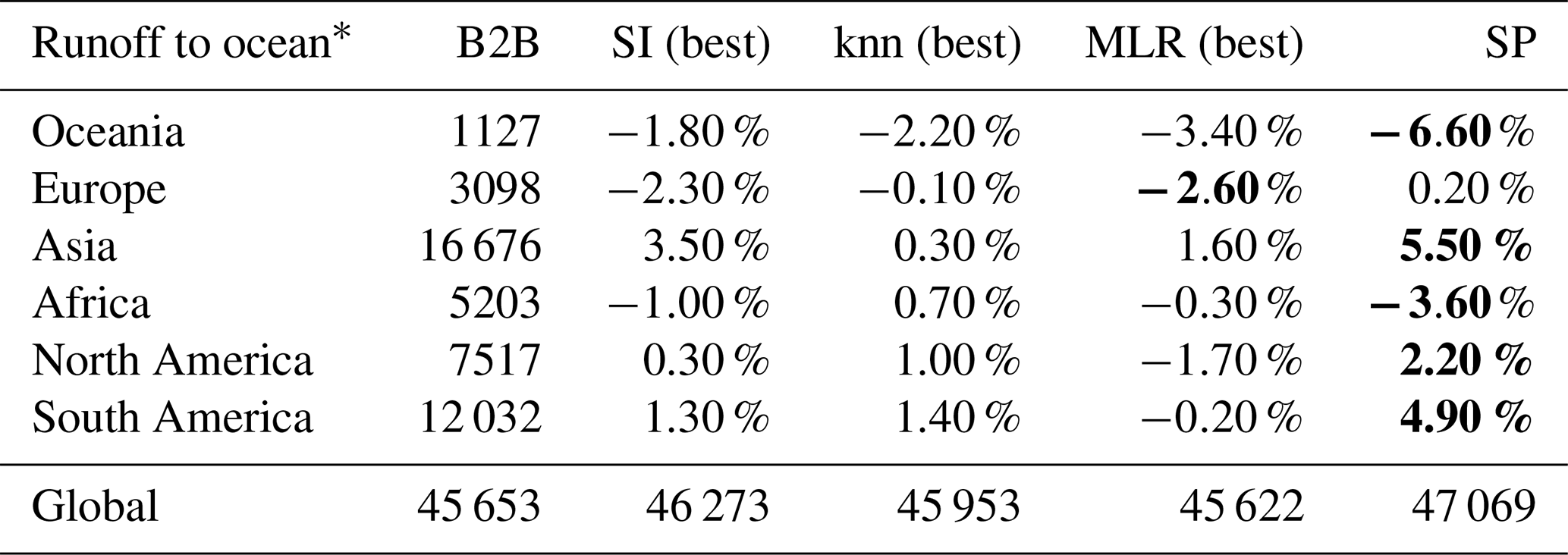
∗ including endorheic basins
The most significant deviations in the continental sums of runoff to ocean in Table 3 are due to SP. Only for Europe is the highest deviation related to MLR (best), not SP. Interestingly, the estimated sums of SP occasionally define the lowest and occasionally the highest extremes for the continents, lacking a systematic pattern. The remarkable role of SP is consistent with previous evaluations in this section, where SP frequently contributes most to the variation in discharge. This suggests that SP may not be suitable for the global scale. Nevertheless, the pseudo-ungauged basins in the split-sample tests may also exhibit considerable distances from the observed basins. Given that SP achieved satisfactory results in both evaluations, using either the logMAE or the KGE, the evaluation indicates the method's suitability on a global scale. Thus, in the future, the split-sample test must be extended to gain deeper insights into the method's robustness and to make a definitive statement about the method's suitability on a global scale. For example, the so-called HDes approach recommended by Lebecherel et al. (2016) could be applied for this purpose. In this approach, the closest basin to the corresponding (pseudo-)ungauged basin is excluded from the regionalization process, thereby enabling an assessment of the method's robustness.
3.5 Challenges and future directions
Regionalization is an inevitable step when parameterizing GHMs. However, only a few studies exist that conduct regionalization experiments with GHMs, often focusing on a single or on two distinct regionalization strategies (e.g., Beck et al., 2016, 2020; Yoshida et al., 2022). A significant challenge in developing and testing different regionalization methods for GHMs is the time-consuming runtime of these models. This extensive runtime impedes comprehensive testing of different regionalization methods, as evaluating the regionalization methods, e.g., using streamflow, demands a considerable number of simulation runs. This study addressed this challenge using the differences between calibrated and regionalized parameter values as an approximator for the suitability of the regionalization methods. Thus, we considered the varying sensitivity of the parameter within the parameter space using the logMAE as the evaluation criterion. Using the differences between calibrated and estimated values is the most straightforward approach, given that WaterGAP3 uses a single calibration parameter, leading to a clear global optimum. However, this approach might not apply to GHMs using multiple calibration parameters due to equifinality. For example, Ayzel et al. (2017) found varying estimated parameter values when regionalizing 11 parameters of the SWAP model using different regionalization methods. They concluded that the difference between regionalized and calibrated values cannot be regarded as a performance measure due to parameter compensation. Thus, further research is required to tackle the challenge of time-consuming GHM run times to enable comprehensive testing of regionalization methods, especially for GHMs using multiple calibration parameters.
Another challenge in regionalizing hydrological models is the optimal selection of predictors for the regionalization methods. Various approaches exist regarding the predictor selection for the regionalization methods (Razavi and Coulibaly, 2013), resulting in a lack of consensus. This study used a predictor selection based on correlation coefficients and an entropy assessment. The results indicate that the approach is particularly well-suited to the similarity indices. However, further research on predictor selection is needed to find the optimal descriptor set per method, as regionalization methods use predictors with varying efficiency. For example, future studies might integrate feature importance bars, e.g., using permutation, to identify the most critical descriptors per method.
Moreover, future research should explicitly account for the issue of multicollinearity. Multicollinearity can affect MLR (and potentially other techniques), resulting in un-generalizable predictions. This phenomenon is more likely to occur when the number of predictor variables is large relative to the number of observation units and when the predictor variables are highly collinear (Kiers and Smilde, 2007). To account for the high importance of the generalizability of regionalization methods for GHMs, we used a high proportion of the basins for testing, i.e., 50 %. Moreover, we used a large sample size (50 % of 933 basins) relative to the number of predictors (maximum 12), lowering the risk of multicollinearity interfering with the results. However, future studies might use methods such as principal component analysis (PCA) or partial least squares (PLS), explicitly accounting for the issue of multicollinearity (e.g., Kroll and Song, 2013). An alternative approach to using PCA or PLS is explicitly testing for multicollinearity in predictor sets using the variance inflation factor and avoiding using predictors with values exceeding a pre-defined threshold (e.g., Kroll et al., 2004).
Valid simulation results from GHMs, such as WaterGAP3, are crucial for detecting hotspots or studying patterns in climate change impacts. However, the lack of worldwide monitoring data makes adapting the GHM parameters for valid global simulations challenging. Therefore, regionalization is necessary to estimate parameters in ungauged basins. This study applies regionalization methods for the first time to WaterGAP3, aiming to provide insights into selecting suitable regionalization methods and evaluating their impact on the runoff simulations. Traditional and machine-learning-based methods are tested to assess the application of several regionalization techniques on a global scale. The concept of benchmark to beat and an ensemble of split-sampling tests are employed for a comprehensive evaluation. Moreover, the impact on runoff simulation is assessed using a wide range of temporal and spatial scales, i.e., from the daily to the yearly and from the local to the global scale.
In this study, four regionalization methods outperform the benchmark to beat in monthly KGE and are thus considered appropriate for WaterGAP3. These methods span the complete range of methodologies, i.e., regression-based methods and methods using the concept of physical similarity and spatial proximity. Moreover, the methods vary in the descriptors used to achieve the highest accuracy. This highlights the fact that different methods use descriptor sets with varying efficiency. All methods perform best when using climatic and physiographic descriptors, indicating that combining climatic and physiographic descriptors is optimal for regionalizing worldwide basins. Mainly for two selected regionalization methods (tuned MLR and knn), the suggested descriptor selection based on correlation coefficients and entropy assessment is not optimal. Further research might integrate variable importance scores or PCA to enhance the predictor selection. Although random forest is known to be especially robust among other machine-learning-based techniques, it shows symptoms of over-parameterization, indicating that the algorithm is too flexible and adjusts to noise in the data, missing the underlying systematic pattern.
Our results demonstrate that variation in the regionalized parameter value does not necessarily lead to variation in river discharge. However, it increases the likelihood that a region's runoff is affected. This spatially varying impact of γ is likely related to the varying sensitivity in ungauged regions regarding γ. Southern South America is a region identified as being especially sensitive to variation in γ. Furthermore, local effects on runoff simulations indicate a temporally varying impact. For example, some impacted rivers indicate a high degree of uncertainty regarding the high percentiles in discharge simulation. These uncertainties potentially lead to a significant impact on flood frequency analysis on a global scale, where the lack of gauging stations in certain regions calls for regionalization. The global impact of regionalization methods that perform well for WaterGAP3 appear to be on the order of minor inter-model differences. This impact rigorously increases when using a poorly performing method for WaterGAP3, underscoring the importance of carefully selecting regionalization methods.
The spatial proximity approach contributes most to the variation in estimated runoff. The remarkable role of this approach suggests that it may not be suitable for the global scale. However, as the pseudo-ungauged basins in the split-sample tests may be located considerably far from the observed basins and the method achieves satisfactory results in all executed evaluations, it is not possible to make a definite statement about the method's suitability for the global scale. Further research is required to gain deeper insights into the methods' robustness, e.g., by extending the analysis by applying the recommended HDes approach (Lebecherel et al., 2016).
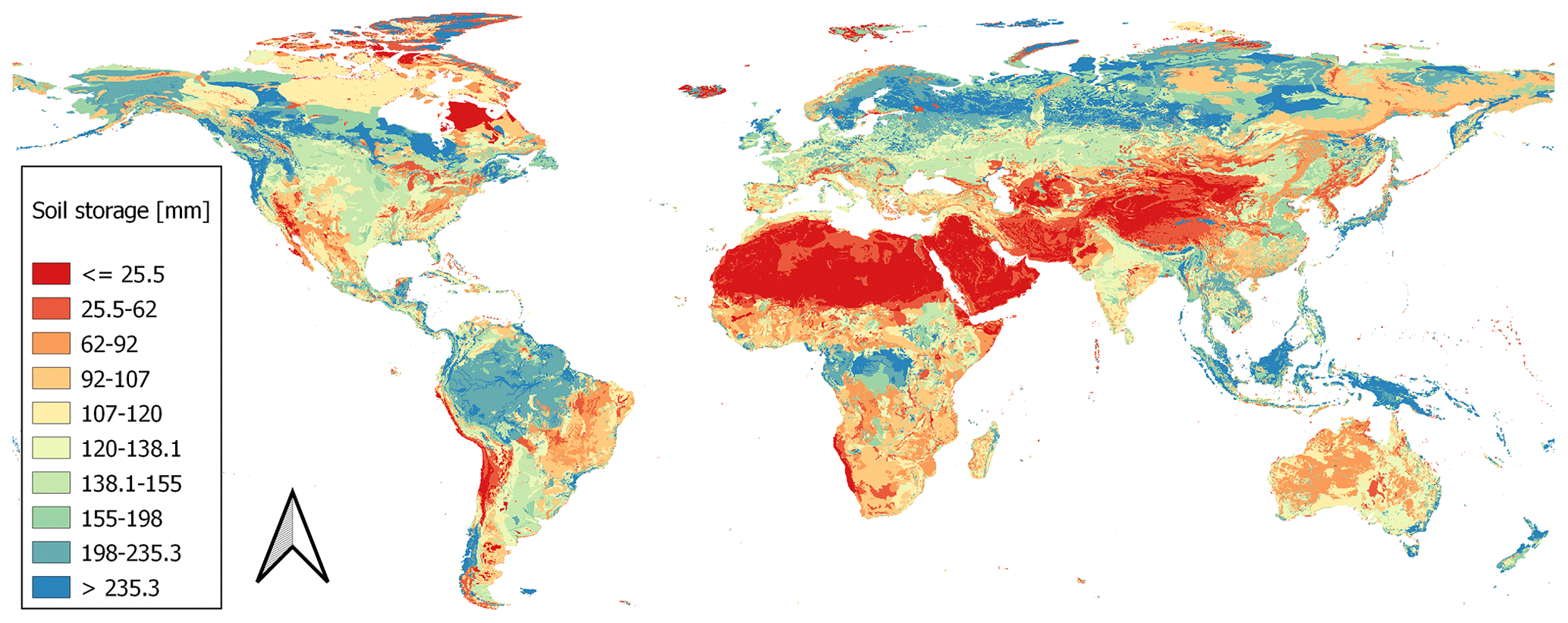
Figure A1Global map of the size of soil storage based on Batjes (2012) and land use information (derived from Friedl and Sulla-Menashe, 2019).
The clustered calibrated parameter values at the extremes of the valid parameter space (see Fig. 1b) are a known problem within the calibration. As the parameter space, i.e., the parameter bounds, is crucial for calibration and, in consequence, for regionalization, we address this issue by a brief sensitivity analysis to demonstrate that the clustering of the calibrated parameter values is more an issue of missing processes (or using additional parameter values) than an issue of inappropriate parameter space. As the lower limit of the calibrated parameter (0.1) is sufficiently small in comparison to other studies using a similar HBV-based approach for runoff generation processes (e.g., see the beta in Table A2 in Jansen et al., 2022), we focus the sensitivity analysis on the upper limit of γ (5.0).
In the sensitivity analysis regarding the upper limit of γ, we applied the model formula (see Eq. B1) containing the model's parameter γ and modified it within the bounds of 0.1 and 10. Additionally, we modified the soil saturation varying from 1 % to 95 %.
The calculated outflow and its relationship to the soil saturation and γ are depicted in Fig. B1. The incoming effective precipitation is defined as constant. As it is a factor in Eq. (B1), the results regarding incoming effective precipitation are linearly scalable.
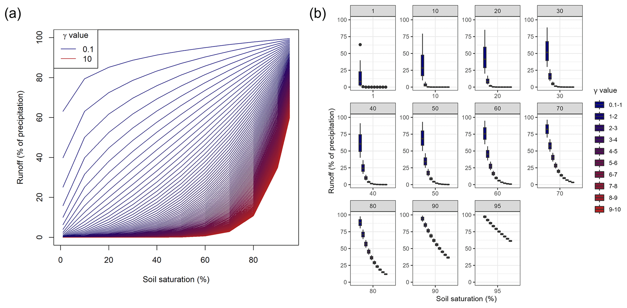
Figure B1(a) Runoff generation in the soil layer (neglecting overflow and evapotranspiration) using different values for the calibration parameter and increasing the soil moisture. (b) Runoff generation for varying soil moisture grouped in bins of size 1.
In the depicted Fig. B1, the runoff generation process differences between differing γ values become more linear when soil saturation increases. Thus, the non-linear model parameter becomes less critical for high soil moisture. Generally, the runoff generation process differences for higher γ values are more pronounced for higher soil moisture. For lower soil moisture, the smaller values have higher effects on the generated runoff. For example, for 70 % soil moisture, the differences for γ values ranging from 5 to 10 are between 3 % and 16 %. For the same soil moisture, the range in runoff generation varies from 16 % to 70 % for γ values between 1 and 5.
High γ values usually occur in dry regions (see Fig. 4b in Müller Schmied et al., 2021). In dry regions, high soil moisture values are not expected to occur frequently (see e.g., Khosa et al., 2020; Oloruntoba et al., 2024, for estimated and measured soil moisture in Africa and Draper et al., 2008, for estimated and measured soil moisture in Australia). It is, therefore, unlikely that higher γ values will significantly enhance the calibration result or decrease the issue of clustered calibrated parameter values at the higher end of the parameter space. More likely, the clustering of calibrated parameter values will be resolved in dry regions by incorporating additional (missing) model processes, such as evaporation from rivers or inaccurate representation of groundwater processes (Eisner, 2016, p. 49). Thus, the parameter bounds of γ (e.g., also used in Eisner, 2016, p. 16; Müller Schmied et al., 2021, 2023) are not changed in this study.
Overview of basins descriptors used in this study. All basin descriptors are derived from the original model input and aggregated with a simple mean method to basin values to produce the same spatial resolution as the calibrated model parameter.
-
Soil storage. The size of the soil storage is, i.e., the maximal water content in the soil reachable for plants (in mm). The information is the product of rooting depth (defined in a lookup table) and the total available water content derived from Batjes (2012).
-
Open waterbodies. The fraction of the area covered with open waterbodies in the basin is given as a percentage. The model input is based on the Global Lakes and Wetlands Database (GLWD; Lehner and Döll, 2004).
-
Wetlands. The fraction of area covered with wetlands in a basin is given in percentage. The model input is based on the GLWD (Lehner and Döll, 2004).
-
Size. This is the size of a basin (in km2).
-
Slope. The mean slope class is calculated as described in Döll and Fiedler (2008) and is based on the Global 30 Arc-Second Elevation (GTOPO30; Earth Resources Observation and Science Center, U.S. Geological Survey, U.S. Department of the Interior, 1997).
-
Altitude. The mean altitude of a basin is given in meters above sea level and is based on GTOPO30 (Earth Resources Observation and Science Center, U.S. Geological Survey, U.S. Department of the Interior, 1997).
-
Forest. The mean fraction of the area covered with forest is given in percentage and derived from MODIS data (Friedl and Sulla-Menashe, 2019), where 2001 is used as a reference. All grid cells having a dominant International Geosphere–Biosphere Program (IGBP) classification between one and five are defined as forest.
-
Sealed area. The mean fraction of sealed area is given in percentage and is derived from MODIS data (Friedl and Sulla-Menashe, 2019), where 2001 is used as a reference. All grid cells having an IGBP classification equal to 13 are defined as containing 60 % of the sealed area. Note that the different treatment of forest and sealed area is based on the required model input; while the land cover is a classified value, the sealed area is a floating-point value.
-
Permafrost and glacier. The mean coverage of permafrost and glacier in a basin is given in percentage. It is based on the World Glacier Inventory and the Circum-Arctic Map of Permafrost and Ground-Ice Conditions.
-
Mean temperature. The mean air temperature is based on the meteorological forcing used to drive the model (Lange, 2019), covering the period 1979 to 2016 and given in degrees Celsius.
-
Yearly precipitation. The yearly precipitation sum is based on the meteorological forcing used to drive the model (Lange, 2019), covering the period 1979 to 2016 and given (in mm).
-
Yearly shortwave downward radiation. The yearly shortwave downward radiation is based on the meteorological forcing used to drive the model (Lange, 2019), covering the period 1979 to 2016 (in W m−2).
The correlation between the defined basin descriptors is shown in Fig. C1. The variation within each basin descriptor for basins used for regionalization is shown in Fig. C2.
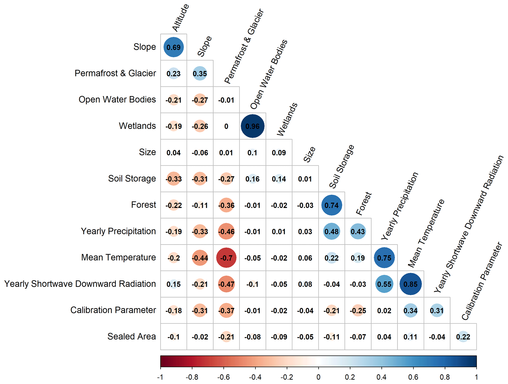
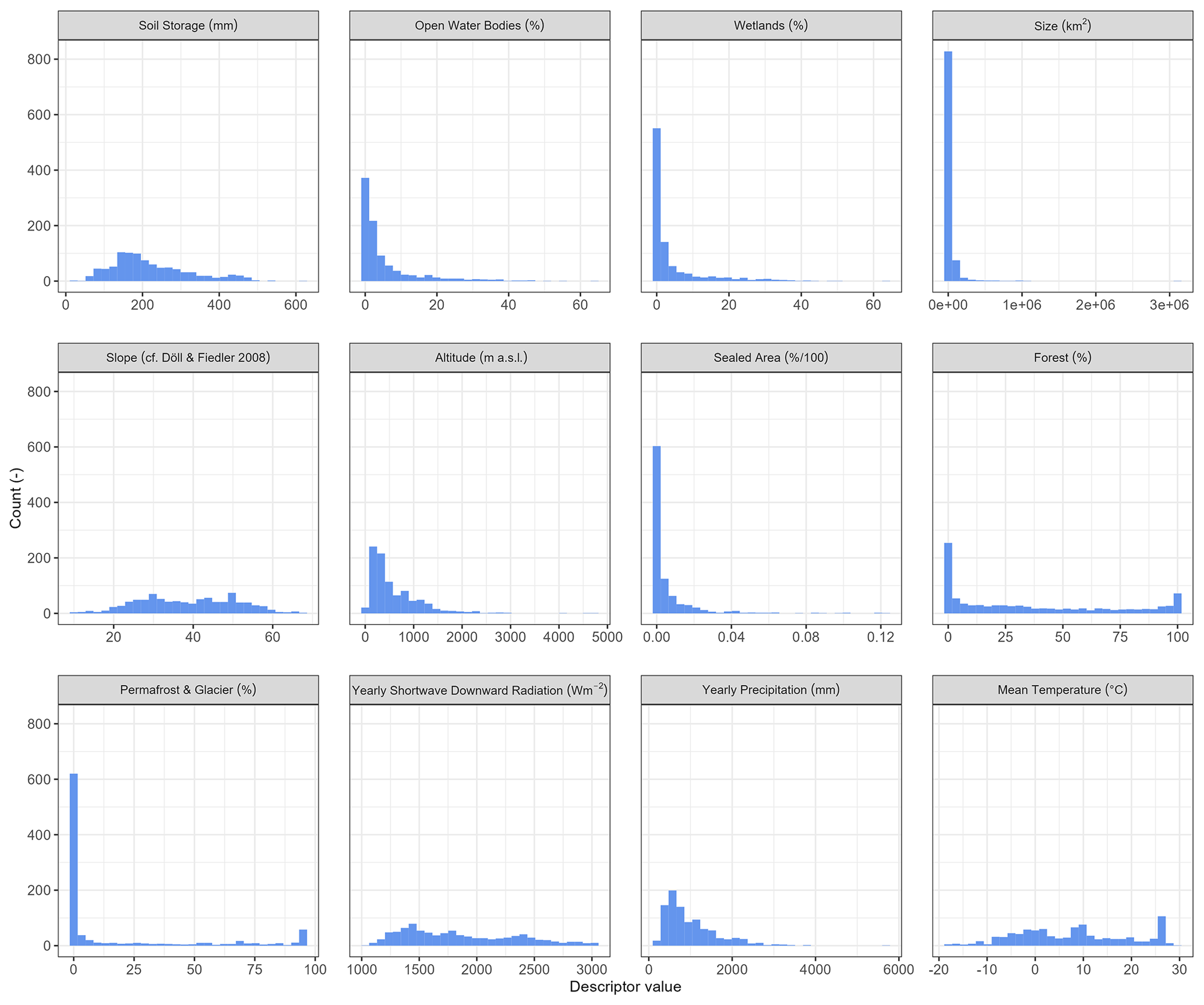
Figure C2Distribution of basin descriptors within all basins used for regionalization (n=933).
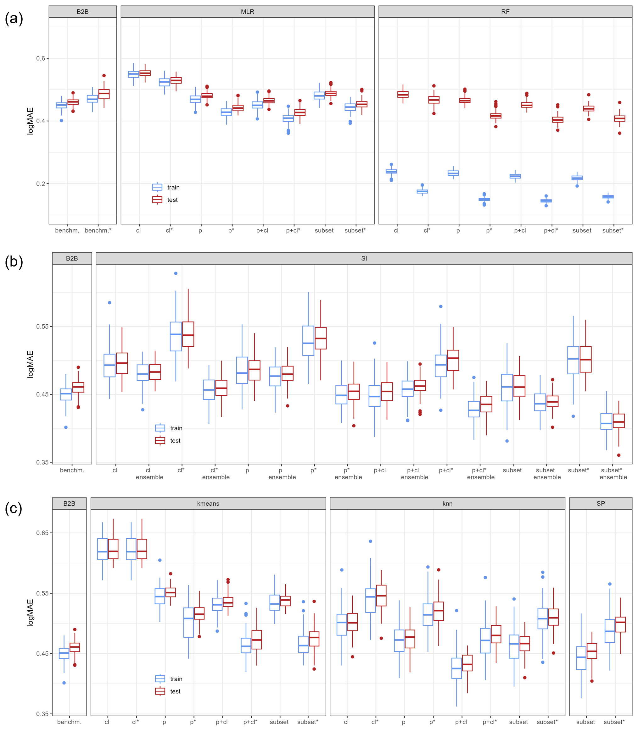
Figure D1The logMAE values for all 100 split-sampling tests using all variants of (a) MLR, RF, and benchmark to beat; (b) SI; and (c) kmeans, knn, and SP. Note that the asterisk (*) indicates the tuned version of the method.
Table D1Performance loss in median logMAE of the ensemble of split-sample tests from training to testing expressed in percentage of logMAE in training.

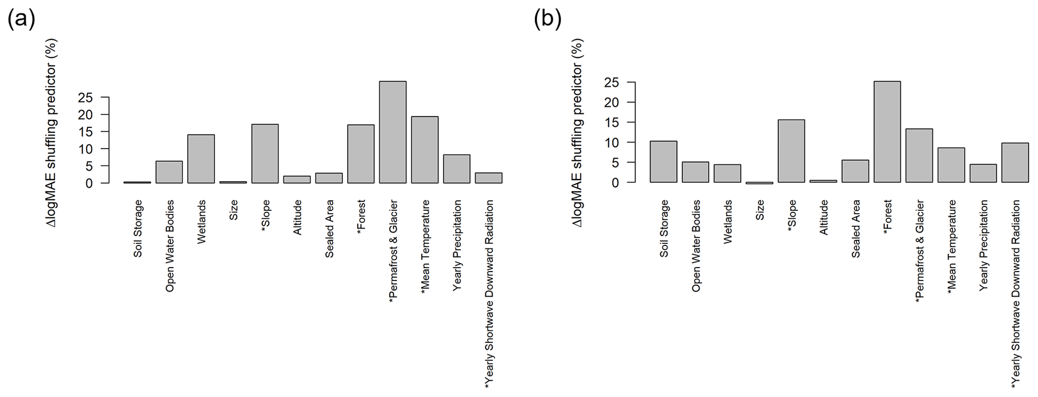
Figure E1Decrease in logMAE for testing using one representative split sample when randomly shuffling each predictor for (a) MLR (best) and (b) knn (best). Note that the asterisk (*) indicates the basin descriptors used in the (weakly) correlated subset.
Krause et al. (2005) suggested a modified version of the NSE that is especially suitable as an overall metric, leading to results between NSE versions focusing on low and high flows. The applied equation for the modified version is given below (see Eq. F1).
where xk is the simulated monthly discharge for the time step k, yk is the observed discharge for the time step k, and μy is the mean of the discharge for the evaluated period.
The evaluation of the modified NSE for all pseudo-ungauged basins of a representative split sample are summarized in Fig. F1. Note that the figure includes also the results of the applied one-sided paired Wilcoxon rank-sum test for the KGE values mentioned in Sect. 3.3.
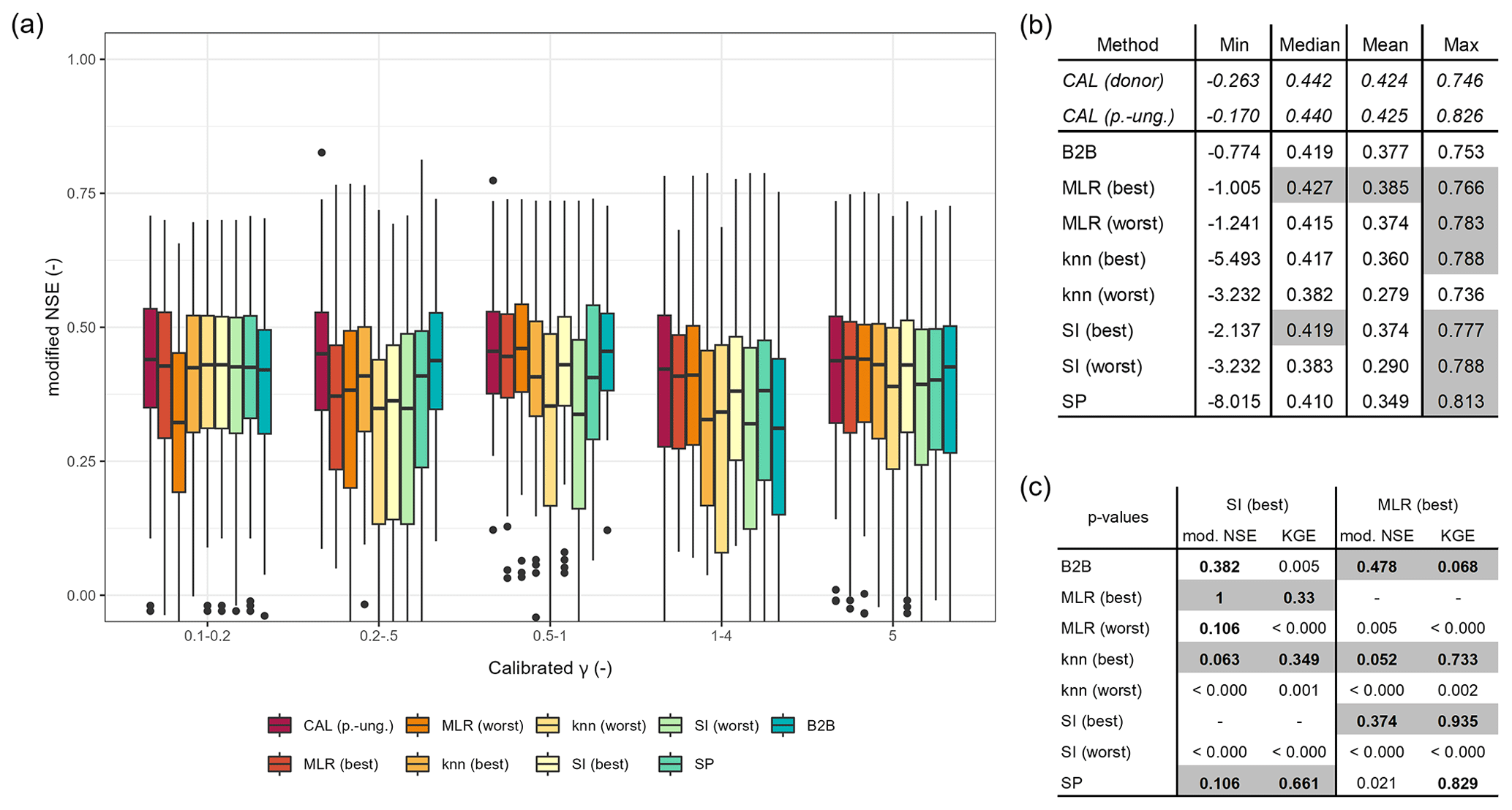
Figure F1(a) Modified NSE values of pseudo-ungauged basins from the split-sample test grouped by the range of calibrated γ values. (b) Selected metrics of modified NSE values from the pseudo-ungauged basins (performance better than or equal to the benchmark to beat is highlighted in gray). (c) The p values of the one-sided paired Wilcoxon rank-sum test, testing the best-performing methods MLR (best) and SI (best) against all other regionalization methods. Note that p values greater than 0.05 are highlighted in bold, indicating that the null hypothesis cannot be rejected; thus the difference in central tendency is not statistically significant. Cases where the results of modified NSE and KGE indicate the same are shaded gray.
The data and supporting R code to reproduce this study's findings are available at https://doi.org/10.5281/zenodo.13122859 (Kupzig, 2024). The data provided in Kupzig (2024) is mainly based on model output from WaterGAP3 (Flörke et al., 2024, https://doi.org/10.5281/zenodo.10940380) using the EWEMBI data set (Lange, 2019, https://doi.org/10.5880/pik.2019.004) and comparing it with the GRDC data set (GRDC, 2020). Appendix C describes the basin characteristics used.
JK developed, designed, and drafted the study. NK helped to design the experiment. MF provided feedback throughout the entire process and supported the writing.
The contact author has declared that none of the authors has any competing interests.
Publisher's note: Copernicus Publications remains neutral with regard to jurisdictional claims made in the text, published maps, institutional affiliations, or any other geographical representation in this paper. While Copernicus Publications makes every effort to include appropriate place names, the final responsibility lies with the authors.
We acknowledge the discharge data from GRDC (The Global Runoff Data Centre, 56068 Koblenz, Germany). We are thankful for the valuable comments of two anonymous referees and Charles Onyutha, who helped improve the paper.
This paper was edited by Charles Onyutha and reviewed by two anonymous referees.
Arheimer, B., Pimentel, R., Isberg, K., Crochemore, L., Andersson, J. C. M., Hasan, A., and Pineda, L.: Global catchment modelling using World-Wide HYPE (WWH), open data, and stepwise parameter estimation, Hydrol. Earth Syst. Sci., 24, 535–559, https://doi.org/10.5194/hess-24-535-2020, 2020.
Arsenault, R. and Brissette, F. P.: Continuous streamflow prediction in ungauged basins: The effects of equifinality and parameter set selection on uncertainty in regionalization approaches, Water Resour. Res., 50, 6135–6153, https://doi.org/10.1002/2013WR014898, 2014.
Ayzel, G. V., Gusev, E. M., and Nasonova, O. N.: River runoff evaluation for ungauged watersheds by SWAP model. 2. Application of methods of physiographic similarity and spatial geostatistics, Water Resour., 4, 547–558, https://doi.org/10.1134/S0097807817040029, 2017.
Barbarossa, V., Bosmans, J., Wanders, N., King, H., Bierkens, M. F. P., Huijbregts, M. A. J., and Schipper, A. M.: Threats of global warming to the world's freshwater fishes, Nat. Commun., 12, 1701, https://doi.org/10.1038/s41467-021-21655-w, 2021.
Batjes, N. H.: ISRIC-WISE derived soil properties on a 5 by 5 arc-minutes global grid (ver. 1.2), ISRIC [data set], https://data.isric.org/geonetwork/srv/eng/catalog.search#/metadata/82f3d6b0-a045-4fe2-b960-6d05bc1f37c0 (last access: 22 June 2020), 2012.
Beck, H. E., van Dijk, A. I. J. M., Roo, A. de, Miralles, D. G., McVicar, T. R., Schellekens, J., and Bruijnzeel, L. A.: Global-scale regionalization of hydrologic model parameters, Water Resour. Res., 52, 3599–3622, https://doi.org/10.1002/2015WR018247, 2016.
Beck, H. E., van Dijk, A. I. J. M., de Roo, A., Dutra, E., Fink, G., Orth, R., and Schellekens, J.: Global evaluation of runoff from 10 state-of-the-art hydrological models, Hydrol. Earth Syst. Sci., 21, 2881–2903, https://doi.org/10.5194/hess-21-2881-2017, 2017.
Beck, H. E., Pan, M., Lin, P., Seibert, J., van Dijk, A. I. J. M., and Wood, E. F: Global Fully Distributed Parameter Regionalization Based on Observed Streamflow From 4,229 Headwater Catchments, J. Geophys. Res.-Atmos., 125, e2019JD031485, https://doi.org/10.1029/2019JD031485, 2020.
Benjamini, Y. and Hochberg, Y.: Controlling the False Discovery Rate: A Practical and Powerful Approach to Multiple Testing, J. Roy. Stat. Soc. B, 57, 289–300, 1995.
Boulange, J, Hanasaki, N, Yamazaki, D., and Pokhrel, Y.: Role of dams in reducing global flood exposure under climate change, Nat. Commun., 12, 417, https://doi.org/10.1038/s41467-020-20704-0, 2021.
Box, G. E. P. and Cox, D. R.: An analysis of transformations, J. Roy. Stat. Soc. B, 26, 211–252, 1964.
Breimann, L.: Random Forests, Mach. Learn., 45, 1–32, https://doi.org/10.1023/A:1010933404324, 2001.
Chaney, N. W., Herman, J. D., Ek, M. B., and Wood, E. F.: Deriving global parameter estimates for the Noah land surface model using FLUXNET and machine learning, J. Geophys. Res.-Atmos., 121, 13218–13235, https://doi.org/10.1002/2016JD024821, 2016.
Charrad, M., Ghazzali, N., Boiteau, V., and Niknafs, A.: NbClust: An R Package for Determining the Relevant Number of Clusters in a Data Set, J. Stat. Softw., 61, 1–36, https://doi.org/10.18637/jss.v061.i06, 2014.
Clark, M. P., Vogel, R. M., Lamontagne, J. R., Mizukami, N., Knoben, W. J. M., Tang, G., Gharari, S., Freer, J. E., Whitfield, P. H., Shook, K., and Papalexiou, S. M.: The abuse of popular performance metrics in hydrologic modelling, Water Resour. Res., 57, e2020WR029001, https://doi.org/10.1029/2020WR029001, 2021.
Cuntz, M., Mai, J., Samaniego, L, Clark, M., Wulfmeyer, V., Branch, O., Attinger, S., and Thober, S.: The impact of standard and hard-coded parameters on the hydrologic fluxes in the Noah-MP land surface model, J. Geophys. Res.-Atmos., 121, 10676–10700, https://doi.org/10.1002/2016JD025097, 2016.
Döll, P. and Fiedler, K.: Global-scale modeling of groundwater recharge, Hydrol. Earth Syst. Sci., 12, 863–885, https://doi.org/10.5194/hess-12-863-2008, 2008.
Döll, P., Kaspar, F., and Lehner, B.: A global hydrological model for deriving water availability indicators: model tuning and validation, J. Hydrol., 270, 105–134, https://doi.org/10.1016/S0022-1694(02)00283-4, 2003.
Döll, P., Hasan, H. M. M., Schulze, K., Gerdener, H., Börger, L., Shadkam, S., Ackermann, S., Hosseini-Moghari, S.-M., Müller Schmied, H., Güntner, A., and Kusche, J.: Leveraging multi-variable observations to reduce and quantify the output uncertainty of a global hydrological model: evaluation of three ensemble-based approaches for the Mississippi River basin, Hydrol. Earth Syst. Sci., 28, 2259–2295, https://doi.org/10.5194/hess-28-2259-2024, 2024.
Draper, C. S., Walker, J. P., Steinle, P. J., de Jeu, R. A. M., and Holmes, T. R. H.: An evaluation of AMSR–E derived soil moisture over Australia, Remote Sens. Environ., 113, 703–710, https://doi.org/10.1016/j.rse.2008.11.011, 2008.
Earth Resources Observation and Science Center, U.S. Geological Survey, U.S. Department of the Interior: USGS 30 ARC-second Global Elevation Data, GTOPO30. Research Data Archive at the National Center for Atmospheric Research, Computational and Information Systems Laboratory [data set], https://doi.org/10.5065/A1Z4-EE71, 1997.
Eisner, S.: Comprehensive Evaluation of the WaterGAP3 Model across Climatic, Physiographic, and Anthropogenic Gradients, Ph.D. thesis, University of Kassel, Kassel, Germany, 128 pp., 2016.
Feigl, M., Thober, S., Schweppe, R., Herrnegger, M., Samaniego, L., and Schulz, K.: Automatic Regionalization of Model Parameters for Hydrological Models, Water Resour. Res., 58, e2022WR031966, https://doi.org/10.1029/2022WR031966, 2022.
Flörke, M., Kynast, E., Eisner, S., Verzano, K., Kupzig, J., Voß, F., Lehner, B., Rivera, J., aus der Beek, T., aus der Beek, M., Malsy, M., and Alcamo, J.: WaterGAP3 (v1.0.0), Zenodo [software], https://doi.org/10.5281/zenodo.10940380, 2024.
Friedl, M. and Sulla-Menashe, D.: MCD12Q1 MODIS/Terra+Aqua Land, Cover Type Yearly L3 Global 500m SIN Grid V006, NASA EOSDIS Land Processes DAAC [data set], https://doi.org/10.5067/MODIS/MCD12Q1.006, 2019.
Golian, S., Murphy, C., and Meresa, H.: Regionalization of hydrological models for flow estimation in ungauged catchments in Ireland, J. Hydrol.-Regional Studies, 36, 100859, https://doi.org/10.1016/j.ejrh.2021.100859, 2021.
GRDC: The Global Runoff Data Centre, 56068 Koblenz, Germany, 2020.
Gudmundsson, L., Tallaksen, L. M., Stahl, K., Clark, D. B., Dumont, E., Hagemann, S., Bertrand, N., Gerten, D., Heinke, J., Hanasaki, N., Voss, F., & Koirala, S.: Comparing Large-Scale Hydrological Model Simulations to Observed Runoff Percentiles in Europe, J. Hydrometeorol., 13, 604–620, https://doi.org/10.1175/JHM-D-11-083.1, 2012.
Guo, Y., Zhang, Y., Zhang, L., and Wang, Z.: Regionalization of hydrological modeling for predicting streamflow in ungauged catchments: A comprehensive review, WIREs Water, 8, e1487, https://doi.org/10.1002/wat2.1487, 2020.
Gupta, H. V., Sorooshian, S., and Yapo, P. O.: Toward improved calibration of hydrologic models: Multiple and noncommensurable measures of information, Water Resour. Res., 34, 751–763, https://doi.org/10.1029/97WR03495, 1998.
Gupta, H. V., Kling, H., Yilmaz, K. K., and Martinez, G. F.: Decomposition of the mean squared error and NSE performance criteria: Implications for improving hydrological modelling, J. Hydrol., 377, 80–91, https://doi.org/10.1016/j.jhydrol.2009.08.003, 2009.
He, Y., Bárdossy, A., and Zehe, E.: A review of regionalisation for continuous streamflow simulation, Hydrol. Earth Syst. Sci., 15, 3539–3553, https://doi.org/10.5194/hess-15-3539-2011, 2011.
Herbert, C. and Döll, P.: Analyzing the informative value of alternative hazard indicators for monitoring drought hazard for human water supply and river ecosystems at the global scale, Nat. Hazards Earth Syst. Sci., 23, 2111–2131, https://doi.org/10.5194/nhess-23-2111-2023, 2023.
Jansen, K. F., Teuling, A. J., Craig, J. R., Dal Molin, M., Knoben, W. J. M., Parajka, J., Vis, M., and Melsen, L. A.: Mimicry of a conceptual hydrological model (HBV): What's in a name?, Water Resour. Res., 57, e2020WR029143, https://doi.org/10.1029/2020WR029143, 2022.
Janssen, P. H. M. and Heuberger, P. S. C.: Calibration of process-oriented models, Ecol. Model., 83, 55–66, https://doi.org/10.1016/0304-3800(95)00084-9, 1995.
Jones, E. R., Bierkens, M. F. P., and van Vliet, M. T. H.: Current and future global water scarcity intensifies when accounting for surface water quality, Nat. Clim. Change, 14, 629–635, https://doi.org/10.1038/s41558-024-02007-0, 2024.
Kaspar, F.: Entwicklung und Unsicherheitsanalyse eines globalen hydrologischen Modells, Ph.D. thesis, University of Kassel, Kassel, Germany, 129 pp., 2004.
Khosa, F. V., Mateyisi, M. J., van der Merwe, M. R., Feig, G. T., Engelbrecht, F. A., and Savage, M. J.: Evaluation of soil moisture from CCAM-CABLE simulation, satellite-based models estimates and satellite observations: a case study of Skukuza and Malopeni flux towers, Hydrol. Earth Syst. Sci., 24, 1587–1609, https://doi.org/10.5194/hess-24-1587-2020, 2020.
Kiers, H. A. L. and Smilde, A. K.: A comparison of various methods for multivariate regression with highly collinear variables, Stat. Meth. Appl., 16, 193–228, https://doi.org/10.1007/s10260-006-0025-5, 2007.
Krabbenhoft, C. A., Allen, G. H., Lin, P., Godsey, S. E., Allen, D. C., Burrows, R. M., DelVecchia, A. G., Fritz, K. M., Shanafield, M., Burgin, A. J., Zimmer, M. A., Datry, T., Dodds, W. K., Jones, C. N., Mims, M. C., Franklin, C., Hammond, J. C., Zipper, S., Ward, A. S., and Olden, J. D.: Assessing placement bias of the global river gauge network, Nat. Sustain., 5, 586–592, https://doi.org/10.1038/s41893-022-00873-0, 2022.
Krause, P., Boyle, D. P., and Bäse, F.: Comparison of different efficiency criteria for hydrological model assessment, Adv. Geosci., 5, 89–97, https://doi.org/10.5194/adgeo-5-89-2005, 2005.
Kroll, C., Lutz, J., Allen, B., and Vogel, R. M.: Developing a Watershed Characteristics Database to Improve Low Streamflow Prediction, J. Hydrol. Eng., 9, 116–125, https://doi.org/10.1061/(ASCE)1084-0699(2004)9:2(116), 2004.
Kroll, C. N. and Song P.: Impact of Multicollinearity on Small Sample Hydrologic Regression Models, Water Resour. Res., 49, 3756–3769, https://doi.org/10.1002/wrcr.20315, 2013.
Kupzig, J.: JKupzig/regionalization_watergap3: Revised Manuscript (v1.1) (v.1.1.2), Zenodo [code and data set], https://doi.org/10.5281/zenodo.13122859, 2024.
Kupzig, J., Reinecke, R., Pianosi, F., Flörke, M., and Wagener, T.: Towards parameter estimation in global hydrological models, Environ. Res. Lett., 18, 74023, https://doi.org/10.1088/1748-9326/acdae8, 2023.
Lange, S.: EartH2Observe, WFDEI and ERA-Interim data Merged and Bias-corrected for ISIMIP (EWEMBI), V. 1.1, GFZ Data Services [data set], https://doi.org/10.5880/pik.2019.004, 2019.
Lebecherel, L., Andréassian, V., and Perrin, C.: On evaluating the robustness of spatial-proximity-based regionalization methods, J. Hydrol., 539, 196–203, https://doi.org/10.1016/j.jhydrol.2016.05.031, 2016.
Lehner, B. and Döll, P: Development and validation of a global database of lakes, reservoirs and wetlands, J. Hydrol., 296, 1–22, https://doi.org/10.1016/j.jhydrol.2004.03.028, 2004.
Lehner, B., Verdin, K., and Jarvis, A.: New global hydrography derived from spaceborne elevation data, Eos, Transactions, AGU, 89, 93–94, https://doi.org/10.1029/2008EO100001, 2008.
Liam, A. and Wiener, M.: Classification and Regression by randomForest, R News, 2, 18–22, 2002.
Lindström, G., Johansson, B., Persson, M., Gardelin, M., and Bergström, S.: Development and test of the distributed HBV-96 hydrological model, J. Hydrol., 201, 272–288, https://doi.org/10.1016/S0022-1694(97)00041-3, 1997.
McIntyre, N, Lee, H., Wheater, H., Young, A., and Wagener, T.: Ensemble predictions of runoff in ungauged catchments, Water Resour. Res., 41, W12434, https://doi.org/10.1029/2005WR004289, 2005.
Merz, R. and Blöschl, G.: Regionalisation of catchment model parameters, J. Hydrol., 287, 95–123, https://doi.org/10.1016/j.jhydrol.2003.09.028, 2004.
Müller Schmied, H., Cáceres, D., Eisner, S., Flörke, M., Herbert, C., Niemann, C., Peiris, T. A., Popat, E., Portmann, F. T., Reinecke, R., Schumacher, M., Shadkam, S., Telteu, C.-E., Trautmann, T., and Döll, P.: The global water resources and use model WaterGAP v2.2d: model description and evaluation, Geosci. Model Dev., 14, 1037–1079, https://doi.org/10.5194/gmd-14-1037-2021, 2021.
Müller Schmied, H., Trautmann, T., Ackermann, S., Cáceres, D., Flörke, M., Gerdener, H., Kynast, E., Peiris, T. A., Schiebener, L., Schumacher, M., and Döll, P.: The global water resources and use model WaterGAP v2.2e: description and evaluation of modifications and new features, Geosci. Model Dev. Discuss. [preprint], https://doi.org/10.5194/gmd-2023-213, in review, 2023.
Nash, J. E. and Sutcliff, J. V.: River flow forecasting through conceptual models part I – A discussion of principles, J. Hydrol., 10, 282–290, https://doi.org/10.1016/0022-1694(70)90255-6, 1970.
Nijssen, B., O'Donnell, G. M., Lettenmeier, D. P., Lohmann, D., and Wood, E. F.: Predicting the Discharge of Global Rivers, Am. Meteorol. Soc., 3307–3323, https://doi.org/10.1175/1520-0442(2001)014<3307:PTDOGR>2.0.CO;2, 2000.
Oloruntoba, B. J., Kollet, S., Montzka, C., Vereecken, H., and Hendricks Franssen, H.-J.: High Resolution Land Surface Modelling over Africa: the role of uncertain soil properties in combination with temporal model resolution, EGUsphere [preprint], https://doi.org/10.5194/egusphere-2023-3132, 2024.
Onyutha, C.: Pros and cons of various efficiency criteria for hydrological model performance evaluation, Proc. IAHS, 385, 181–187, https://doi.org/10.5194/piahs-385-181-2024, 2024.
Oudin, L., Andréassian, V., Perrin, C., Michel, C., and Le Moine, N.: Spatial proximity, physical similarity, regression and ungaged catchments: A comparison of regionalization approaches based on 913 French catchments, Water Resour. Res., 44, W03413, https://doi.org/10.1029/2007WR006240, 2008.
Oudin, L., Kay, A., Andréassian, V., and Perrin, C.: Are seemingly physically similar catchments truly hydrologically similar?, Water Resour. Res., 46, W11558, https://doi.org/10.1029/2009WR008887, 2010.
Pagliero, L., Bouraoui, F., Diels, J., Willems, P., and McIntyre, N.: Investigating regionalization techniques for large-scale hydrological modelling, J. Hydrol., 570, 220–235, https://doi.org/10.1016/j.jhydrol.2018.12.071, 2019.
Parajka, J., Merz, R., and Blöschl, G.: A comparison of regionalisation methods for catchment model parameters, Hydrol. Earth Syst. Sci., 9, 157–171, https://doi.org/10.5194/hess-9-157-2005, 2005.
Poissant, D., Arsenault, R., and Brissette, F.: Impact of parameter set dimensionality and calibration procedures on streamflow prediction at ungauged catchments, J. Hydrol.-Regional Studies, 12, 220–237, https://doi.org/10.1016/j.ejrh.2017.05.005, 2017.
Pool, S., Vis, M., and Seibert, J.: Regionalization for ungauged catchments – Lessons learned from a comparative large-sample study, Water Resour. Res., 57, e2021WR030437, https://doi.org/10.1029/2021WR030437, 2021.
Qi, W., Chen, J., Li, L., Xu, C., Li, J., Xiang, Y., and Zhang, S.: A framework to regionalize conceptual model parameters for global hydrological modeling, Hydrol. Earth Syst. Sci. Discuss. [preprint], https://doi.org/10.5194/hess-2020-127, 2020.
Razavi, T. and Coulibaly, P.: Streamflow Prediction in Ungauged Basins: Review of Regionalization Methods, J. Hydrol. Eng., 18, 958–975, https://doi.org/10.1061/(ASCE)HE.1943-5584.0000690, 2013.
R Core Team.: R: A language and environment for statistical computing R Foundation for Statistical Computing, Vienna, Austria, https://www.r-project.org/ (last access: 9 September 2023), 2020.
Reichl, J. P. C., Western, A. W., McIntyre, N. R., and Chiew, F. H. S.: Optimization of a Similarity Measure for Estimating Ungauged Streamflow, Water Resour. Res., 45, W10423, https://doi.org/10.1029/2008WR007248, 2009.
Ritter, A. and Muñoz-Carpena, R.: Performance evaluation of hydrological models: Statistical significance for reducing subjectivity in goodness-of-fit assessments, J. Hydrol., 480, 33–45, https://doi.org/10.1016/j.jhydrol.2012.12.004, 2013.
Samaniego, L., Kumar, R., and Attinger, S.: Multiscale parameter regionalization of a grid-based hydrologic model at the mesoscale, Water Resour. Res., 46, W05523, https://doi.org/10.1029/2008WR007327, 2010.
Schaefli, B. and Gupta, H. V.: Do Nash values have value?, Hydrol. Process., 21, 2075–2080, https://doi.org/10.1002/hyp.6825, 2007.
Schweppe, R., Thober, S., Müller, S., Kelbling, M., Kumar, R., Attinger, S., and Samaniego, L.: MPR 1.0: a stand-alone multiscale parameter regionalization tool for improved parameter estimation of land surface models, Geosci. Model Dev., 15, 859–882, https://doi.org/10.5194/gmd-15-859-2022, 2022.
Seibert, J.: On the need for benchmarks in hydrological modelling, Hydrol. Process., 15, 1063–1064, https://doi.org/10.1002/hyp.446, 2001.
Seibert, J., Staudinger, M., and van Meerveld, H. J. I.: Validation and Over-Parameterization – Experiences from Hydrological Modeling, in: Computer Simulation Validation, edited by: Breisbart, C. and Saam, J. S., Springer Nature Switzerland, Cham, Switzerland, 811–834, https://doi.org/10.1007/978-3-319-70766-2, 2019.
Shannon, C. E.: A Mathematical Theory of Communication, The Bell System Technical Journal, 3, 379–423, https://doi.org/10.1002/j.1538-7305.1948.tb01338.x, 1948.
Stacke, T. and Hagemann, S.: HydroPy (v1.0): a new global hydrology model written in Python, Geosci. Model Dev., 14, 7795–7816, https://doi.org/10.5194/gmd-14-7795-2021, 2021.
Tang, Y., Marshall, L., Sharma, A., and Smith, T.: Tools for investigating the prior distribution in Bayesian hydrology, J. Hydrol., 538, 551–562, https://doi.org/10.1016/j.jhydrol.2016.04.032, 2016.
Tilahun, A. B., Dürr, H. H., Schweden, K., and Flörke, M.: Perspectives on total phosphorus response in rivers: Examining the influence of rainfall extremes and post-dry rainfall, Sci. Total Environ., 940, 173677, https://doi.org/10.1016/j.scitotenv.2024.173677, 2024.
Tongal, H. and Sivakumar, B.: Cross-entropy clustering framework for catchment classification, J. Hydrol., 552, 433–446, https://doi.org/10.1016/j.jhydrol.2017.07.005, 2017.
Venables, W. N. and Ripley, B. D.: Modern Applied Statistics with S (Fourth Edition). Springer Science+Business Media New York, USA, 501 pp., ISBN 978-1-4419-3008-8, 2002
Wagener, T., Wheater, H. S., and Gupta, H. V.: Rainfall – Runoff Modelling in Gauged and Ungauged Catchments, Imperial College Press, London, UK, 332 pp., https://doi.org/10.1142/p335, 2004.
Wagener, T. and Wheater, H. S.: Parameter estimation and regionalization for continuous rainfall-runoff models including uncertainty, J. Hydrol., 320, 132–154, https://doi.org/10.1016/j.jhydrol.2005.07.015, 2006.
Ward, P. J., Jongman, B., Sperna Weiland, F., Bouwman, A., Van Beek, R., Bierkens, M. F. P., Ligtvoet, W., and Winsemius, H. C.: Assessing flood risk at the global scale: model setup, results, and sensitivity, Environ. Res. Lett., 8, 044019, https://doi.org/10.1088/1748-9326/8/4/044019, 2013.
Widén-Nilsson, E., Halldin, S., and Xu, C.: Global water-balance modelling with WASMOD-M: Parameter estimation and regionalisation, J. Hydrol., 340, 105–118, https://doi.org/10.1016/j.jhydrol.2007.04.002, 2007.
Wu, H., Zhang, J., Bao, Z., Wang, G., Wang, W., Yang, Y., and Wang, J.: Runoff Modeling in Ungauged Catchments Using Machine Learning Algorithm-Based Model Parameters Regionalization Methodology, Engineering, 28, 93–104, https://doi.org/10.1016/j.eng.2021.12.014, 2023.
Yang, X., Magnusson, J., Huang, S., Beldring, S., and Xu, C.: Dependence of regionalization methods on the complexity of hydrological models in multiple climatic regions, J. Hydrol., 582, 124357, https://doi.org/10.1016/j.jhydrol.2019.124357, 2020.
Yoshida, T., Hanasaki, N, Nishina, K., Boulange, J, Okada, M., and Troch, P. A.: Inference of Parameters for a Global Hydrological Model: Identifiability and Predictive Uncertainties of Climate-Based Parameters, Water Resour. Res., 58, e2021WR03066, https://doi.org/10.1029/2021WR030660, 2022.
- Abstract
- Introduction
- Data and methods
- Results and discussion
- Conclusion
- Appendix A: Global map of derived global soil moisture storage
- Appendix B: Further analysis regarding the clustering of parameter values at the extremes
- Appendix C: Basin descriptors
- Appendix D: Results of the ensemble of the split-sample tests
- Appendix E: Feature importance bars for MLR (best) and knn (best) using the descriptor set p+cl
- Appendix F: Model performance for pseudo-ungauged basins using a modified version of the NSE
- Code and data availability
- Author contributions
- Competing interests
- Disclaimer
- Acknowledgements
- Review statement
- References