openAMUNDSEN v1.0: an open-source snow-hydrological model for mountain regions

openAMUNDSEN (the open source version of the Alpine MUltiscale Numerical Distributed Simulation ENgine) is a fully distributed snow-hydrological model, designed primarily for calculating the seasonal evolution of snow cover and melt rates in mountain regions. It resolves the mass and energy balance of snow-covered surfaces and layers of the snowpack, thereby including the most important processes that are relevant in complex mountain topography. The potential model applications are very versatile; typically, it is applied in areas ranging from the point scale to the regional scale (i.e., up to some thousands of square kilometers) using a spatial resolution of 10–1000 m and a temporal resolution of 1–3 h or daily. Temporal horizons may vary between single events and climate change scenarios. The openAMUNDSEN model has already been used for many applications, which are referenced herein. It features a spatial interpolation of meteorological observations, several layers of snow with different density and liquid-water contents, wind-induced lateral redistributions, snow–canopy interactions, glacier ice responses to climate, and more. The model can be configured according to each specific application case. A basic consideration for its development was to include a variety of process descriptions of different complexity to set up individual model runs which best match a compromise between physical detail, transferability, simplicity, and computational performance for a certain region in the European Alps, typically a (preferably gauged) hydrological catchment. The Python model code and example data are available as an open-source project on GitHub (https://github.com/openamundsen/openamundsen, last access: 1 June 2024).

1 Introduction

The seasonal evolution of the mountain snow cover has a significant impact on the water regime, the microclimate, and the ecology of mountain catchments and the downstream river regions (Viviroli et al., 2020; Mott et al., 2023). Snow-dominated regions are hence crucial for their inhabitants, with their function of collecting, storing, and releasing water resources: more than one-sixth of the earth's population relies on seasonal snowpacks (and glaciers) for their water supply (Barnett et al., 2005).

The quantification and prediction of snowmelt amount and dynamics are challenging tasks since the complex processes of accumulation, re-distribution, and ablation of snow lead to a high variability in terms of the water distribution in the mountain snow cover in both space and time (Viviroli et al., 2007). This high variability challenges both the measuring and modeling of the height and of the water amount of snow (Vionnet et al., 2022), but the understanding of the consequences of climate change on the hydrological effects of a changing mountain snow cover requires an accurate representation of all related processes (Hanzer et al., 2018). Relevant expected changes imply all kinds of consequences regarding the water supply for public and private sectors, including hydropower generation, agriculture, forestry, and domestic use. Snow processes thereby operate on a variety of spatial and temporal scales (Blöschl, 1999). Further challenges for the modeling of snow processes in mountain regions are imposed by the presence of a forest canopy (Essery et al., 2009; Rutter et al., 2009), which is expected to adapt to the changing climatic conditions and, hence, to have its hydrological effects on the melt rates and the runoff regime from forested mountain regions be altered (Strasser et al., 2011). Finally, the mountain snow cover is an important seasonal landscape feature for all kinds of winter touristic activities (Hanzer et al., 2020).

Several types of models with various levels of complexity have been developed to predict the accumulation and ablation of the mountain snow cover (for an overview, see Mott et al., 2023). Conceptual models mostly rely on temperature as a proxy for melt rates; their parameters are usually fitted to given streamflow observations (Seibert and Bergström, 2022). Such calibrated temperature index models can provide quite accurate results since temperature is a physically meaningful replacement for the important energy sources at the snow surface (Ohmura, 2001). Furthermore, temperature is a mostly available observation and is comparably handy to be interpolated between local recordings. This type of model has been extended, with further elements contributing to the energy balance of the snow surface in various forms. For example, Pellicciotti et al. (2005) included potential solar radiation and parameterized albedo of the snow surface in the modeling, allowing for sub-daily time steps in the calculations.

The most sophisticated type of snow model solves the energy balance of the snow surface, requiring a more-or-less-complex description of the shortwave and longwave radiative fluxes, the turbulent fluxes of sensible and latent heat, the advective heat flux supplied by solid or liquid precipitation, and the soil heat flux at the lower boundary of the snowpack. To solve the energy balance equation, these models divide the snowpack into several layers and iteratively compute the state variables for each single layer, usually including the respective snow height, density, liquid-water content, and temperature (e.g., Vionnet et al., 2012; Lehning et al., 1999; Essery, 2015). Sophisticated model concepts of this type also include methods for the correction of the effect of atmospheric stability on the turbulent fluxes (e.g., Sauter et al., 2020).

For distributed snow model applications in complex mountain terrain, shadowing of the solar radiation beam and – depending on the application and the considered scale – lateral snow redistribution processes like blowing snow or snow slides should be considered in the modeling, especially if simulations are conducted for longer time horizons (e.g., Vionnet et al., 2021; Quéno et al., 2024). Distributed model applications also require sophisticated methods for the spatial interpolation of the local meteorological station recordings (see, e.g., MeteoIO; Bavay and Egger, 2014) or downscaling procedures to utilize gridded weather or climate model outputs to force the simulations.

Very recently, methods of artificial intelligence have undergone a hype-like push regarding the development of new modeling approaches: these make use of the forcing variables governing any processes changing a system and time series of observations of its state. From a certain perspective, these models are similar to calibrated models, with empiricism thereby being replaced by statistics. However, the same limitations exist for such statistical approaches as for the empirical ones in terms of the transferability of their application in space and time. There have also been first attempts to complement complex physical snow models with data-driven machine learning approaches, e.g., the “Deep Learning national scale 1 km resolution snow water equivalent (SWE) prediction model” (https://github.com/whitelightning450/SWEML, last access: 1 June 2024). Similar developments have been undertaken in the field of weather forecasting (e.g., Lam et al., 2023), with respective implications for the predictability of the snow cover evolution. It can be expected that, in this domain, many innovations will emerge in the near future.

Most of the sophisticated energy balance snow (hydrological) models which are currently in development are available as open-source projects, e.g., Surfex (https://www.umr-cnrm.fr/surfex, last access: 1 June 2024); CRHM (https://github.com/CentreForHydrology/CRHM, last access: 1 June 2024); FSM (https://github.com/RichardEssery/FSM, last access: 1 June 2024), SNOWPACK (https://snowpack.slf.ch, last access: 1 June 2024); COSIPY (https://github.com/cryotools/cosipy, last access: 1 June 2024); or, as described in the following, openAMUNDSEN (https://github.com/openamundsen/openamundsen, last access: 1 June 2024).

openAMUNDSEN v1.0, the snow-hydrological model described herein, compromises many of the presented snow model principles, from simple empirical approaches to coupled energy and mass balance calculations. The model is mainly built upon a comprehensive, physically based description of snow processes that are typical for high mountain regions. In particular, the main features of the model include the following:

• spatial interpolation of scattered meteorological point measurements considering elevation using a combined regression–inverse distance weighting (IDW) procedure;

• calculation of solar radiation taking into account terrain slope and orientation, hill-shading, and atmospheric-transmission losses, as well as gains due to scattering, absorption, and multiple reflections between the snow surface and clouds;

• adjustment of precipitation using several correction functions for wind-induced undercatch and lateral redistributions of snow using terrain-based parameterizations;

• simulation of the snow and ice mass and energy balance using either a multilayer scheme or a bulk scheme using four separate layers for new snow, old snow, firn, and ice;

• alternatively, a temperature index and/or enhanced temperature index method, with the latter considering the potential solar radiation and albedo of the surface;

• usage of arbitrary time steps (e.g., 10 min, hourly, or daily) while resampling forcing data to the desired temporal resolution;

• flexible output of time series including arbitrary model variables for selected point locations in NetCDF or CSV format;

• flexible output of gridded model variables, either for specific dates or periodically (e.g., daily or monthly), optionally aggregated to averages or totals in NetCDF, GeoTIFF, or ASCII grid format;

• built-in generation of future meteorological data time series as model forcing with a given trend using a bootstrapping algorithm for the available historical time series of the meteorological recordings;

• live-view window for the visualization of selectable variables of the model state during runtime.

Together with the model, a comprehensive set of data that can be used to run the model for the upper Rofental (Ötztal Alps, Austria – 98.1 km²) is available at PANGAEA (https://doi.org/10.1594/PANGAEA.876120, Strasser et al., 2017, 2018) and at https://doi.org/10.5880/fidgeo.2023.037 (Department of Geography, University of Innsbruck, 2024). Further, an openAMUNDSEN example setup is available at https://doi.org/10.5281/zenodo.13740611 (Hanzer et al., 2024a). These data can be used to set up and run the model for this catchment and to conduct a multitude of simulation experiments like sensitivity tests and evaluations; they can also serve as example to be replaced by data from other catchments or sites. The Rofental is also used in the following as a demonstration site to illustrate the functionalities of the model.

2 Model evolution

The AMUNDSEN model has a development history of well over 20 years. Originally, the model was prepared to compute fields of meteorological variables, snow albedo, and melt with a new enhanced temperature index approach (Pellicciotti et al., 2005). Later, a simple surface energy balance method based on ESCIMO¹ (Strasser and Mauser, 2001) was integrated. The model was then applied and continuously improved to simulate snow hydrological variables for Haut Glacier d'Arolla (Strasser et al., 2004) and the high-alpine region of the Berchtesgaden National Park (Strasser, 2008). Strasser et al. (2008) investigated the sublimation losses of the alpine snow cover from the ground and vegetated surfaces, as well as during blowing-snow events. In Strasser et al. (2011), snow–canopy processes were modeled for a chess-board pattern of various forest stands and open areas on an idealized mountain. The simple bulk energy balance core of the model also exists as a spreadsheet-based point-scale scheme where only hourly meteorological variables have to be pasted in to run the snow simulations for a particular observation site (Strasser and Marke, 2010). This spreadsheet-based model was later extended by the snow–canopy interaction processes that were already implemented in AMUNDSEN (Marke et al., 2016). The energy balance approach was continuously further developed, e.g., with an iterative procedure to account for atmospheric stability (after Weber, 2008) or with the introduction of a four-layer scheme (new snow, old snow, firn, glacier ice; Hanzer et al., 2016). Hanzer et al. (2014) developed a module for the production of technical snow on skiing slopes. Historical and future snow conditions for Austria were determined with the model by Marke et al. (2015) and Marke et al. (2018). Hanzer et al. (2016) presented a parameterization for lateral snow redistribution based on topographic openness and multilevel spatiotemporal validation as a systematic, independent, complete, and redundant validation procedure. The hydrological response and glacier evolution in a changing climate were investigated by Hanzer et al. (2018) for the Ötzal Alps in Austria. Modeled SWE also provided a reference for the fusion with satellite-data-derived snow distribution maps in a machine learning framework (De Gregorio et al., 2019a, b) or to determine the distributed glacier mass balance (Podsiadło et al., 2020). Pfeiffer et al. (2021) used the model to compute the amount of liquid water provided for infiltration by snowmelt and rainfall to determine the conditions that fostered the motion of a landslide in the Tyrolean Alps. With the transition to the open-source project openAMUNDSEN, the multilayer approach by Essery (2015) was integrated into the model as a further alternative to compute the mass and energy balance of a layered snowpack. Finally, the openAMUNDSEN model has been used to simulate the entire process of snow management and the snow conditions for the slopes in skiing areas (Hanzer et al., 2020; Ebner et al., 2021).

The first distributed version of the AMUNDSEN model was developed in IDL (Interactive Data Language; see https://www.nv5geospatialsoftware.com/Products/IDL, last access: 1 June 2024), originally documented in Strasser (2008) and – in a more recent evolutionary stage – in Hanzer et al. (2018). Recently, the model code was completely re-programmed in Python and transferred into an open-source project (https://github.com/openamundsen/openamundsen, last access: 1 June 2024); this was the moment when the model was renamed to openAMUNDSEN. An online documentation is currently in production (https://doc.openamundsen.org, last access: 1 June 2024). New developments which are not yet available online in the GitHub repository will be published there after comprehensive testing.

3 Model concept

3.1 General structural design

The fundamental principles and most important capabilities of the model are shown in the general overview (Fig. 1a). The region for which openAMUNDSEN is to be set up is a rectangle comprised by a digital elevation model (DEM) in raster format. This DEM defines the extent and resolution at which the model computations are performed. The model is capable of simulating the mass balance of both snow and/or glacier ice surfaces, as well as the lateral redistribution of snow, snow–canopy interaction, and evapotranspiration from different land cover types. Irregular observations of meteorological stations or gridded outputs from any kind of raster model are distributed over the domain by means of an IDW procedure considering the dependence on elevation in each time step and spatially interpolated local residuals of the recordings (Fig. 1b); alternatively, fixed monthly gradients can be applied. Several approaches of varying complexity are available to compute surface melt, from a simple temperature index method over an enhanced index approach considering temperature, potential solar radiation, and albedo to sophisticated energy balance methods (Fig. 1c). These melt approaches can be combined with two layering schemes in a total of four different snow model configurations. Each of these configurations can be applied to forest conditions, where a modified set of the meteorological variables is provided to account for the effect of the trees on the inside-canopy microclimatic conditions, parameterized by means of the leaf area index (LAI) as the variable describing the characteristics of the forest (Fig. 1d).

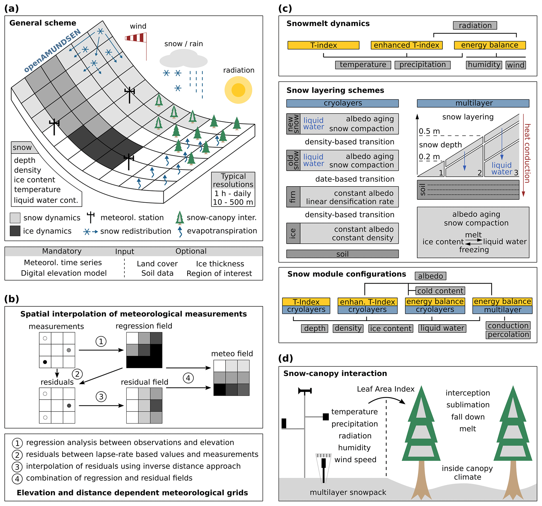
Figure 1 Schematic representation of a domain modeled with the snow-hydrological model openAMUNDSEN (a), spatial interpolation of the meteorological measurements (b), snowmelt dynamics and snow-layering schemes (c), and scaling of observations to inside-canopy meteorological conditions for the simulation of snow–canopy interaction processes (d) in the model.

To save computational time, it is possible to define an irregular region of interest (ROI; i.e., a sub-quantity of pixels); outside this area only, some calculations required for the interpolation of the meteorological variables will be computed (Fig. 2a). Typically, a ROI is a watershed area for which water balance components are aggregated from the single-pixel values so that resulting streamflow volume can be compared to gauge recordings (Hanzer et al., 2018). Weather stations to be considered can also be located outside the ROI or even outside the DEM area; however, in the latter case, they cannot be considered for the determination of shadow areas or regional-scale albedo, which is used to estimate the diffuse radiative fluxes by means of multiple scattering between the surface and the atmosphere. The extent and resolution of the DEM defines the cell size and the geometry of all other raster layers produced in the simulations (Fig. 2b). From this DEM, several derived variables such as slope, aspect, and sky view factor are calculated (Fig. 2c). The sky view factor is the ratio of the visible sky that can be seen from a pixel location to the entire hemisphere that contains both visible and obstructed sky.

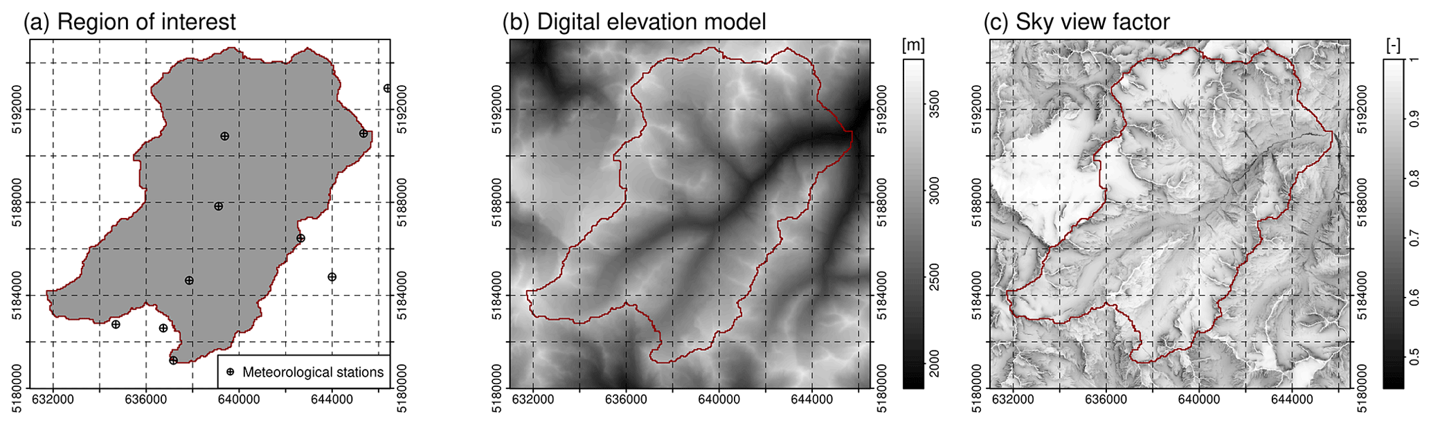
Figure 2 Region of interest (ROI) of the openAMUNDSEN example application to the Rofental (Ötztal Alps, Austria), with locations of weather stations inside and outside this region of interest (a), digital elevation model (b), and sky view factor (c). The red line is the watershed divide of the Rofental for the gauge at Vent (1891 m a.s.l.).

The meteorological forcing for the simulations typically consists of time series of temperature, relative humidity, precipitation, global radiation, and wind speed. These variables are standard observations at the meteorological stations of operational weather services and are mostly available for many mountain regions (e.g., in Austria: http://www.geosphere.at, last access: 1 June 2024). To accurately track the daily course of radiative energy – usually the most important component of the energy for melt (Strasser et al., 2004) – the time step in the modeling in most applications is hourly. To save computational time, the model computations can also be limited to 2- or 3-hourly time steps. If the optional temperature index approach is selected, the time step also can be set to daily. For the case where specific submodules are activated for a model run (e.g., snow–canopy interaction or evapotranspiration), various other spatial input fields have to be prescribed (e.g., land cover, soil, and/or catchment boundaries).

When using meteorological station data as input, the minimum number of stations required is one. This station should provide a continuous series of measurements without gaps. If more than one weather station exists, missing values at a particular site are replaced by the respective results from the interpolation procedure. Where recordings exist, the interpolated values might differ slightly due to the difference in altitude between the exact location of the station and the grid pixel in which it is located (and for which the meteorological field is interpolated). As an alternative to station recordings, it is also possible to provide pre-processed gridded meteorological fields as input to the model, e.g., output data from numerical weather prediction or climate models. Time series data of future climate evolutions that are used to force openAMUNDSEN for climate change scenario simulations can be produced by means of a stochastic block bootstrap resampler, which is realized as an external routine in Python (see Appendix A).

The model simulations are performed for each pixel and each time step (Fig. 3). Prior to these pixel-wise computations for the raster domain, a set of general computations for the model run are performed: after reading the input data, the terrain parameters are computed from the DEM, and precipitation correction parameters are computed (as described in Sect. 3.5). Then the time-dependent computations for all pixels of the domain start, running in a loop from the first to the last time step of the particular simulation run. Several modules are subject to options which can be set in a configuration file in text format.

The results of the computations can be written to the file either as time series for an arbitrary number of pixels (in NetCDF or CSV format) or as gridded model variables for specific selected dates or periodically (e.g., daily, monthly, or yearly), optionally aggregated to averages or totals. Possible formats include NetCDF, GeoTIFF, and ASCII grid.

To keep the modeling time to a minimum, state variables (e.g., from a spin-up simulation) can be imported as raster grids to initialize an openAMUNDSEN model run. Some state variables can also be computed prior to the model run. For example, if glacier outlines are available, the initial ice thickness distribution can be calculated using the approach by Huss and Farinotti (2012). Volumetric balance fluxes of individual glaciers can be calculated from mass balance gradients and constants. Surface elevations and glacier outlines are usually published in glacier inventories (https://wgms.ch/, last access: 1 June 2024), e.g., for Austria in Fischer et al. (2015).

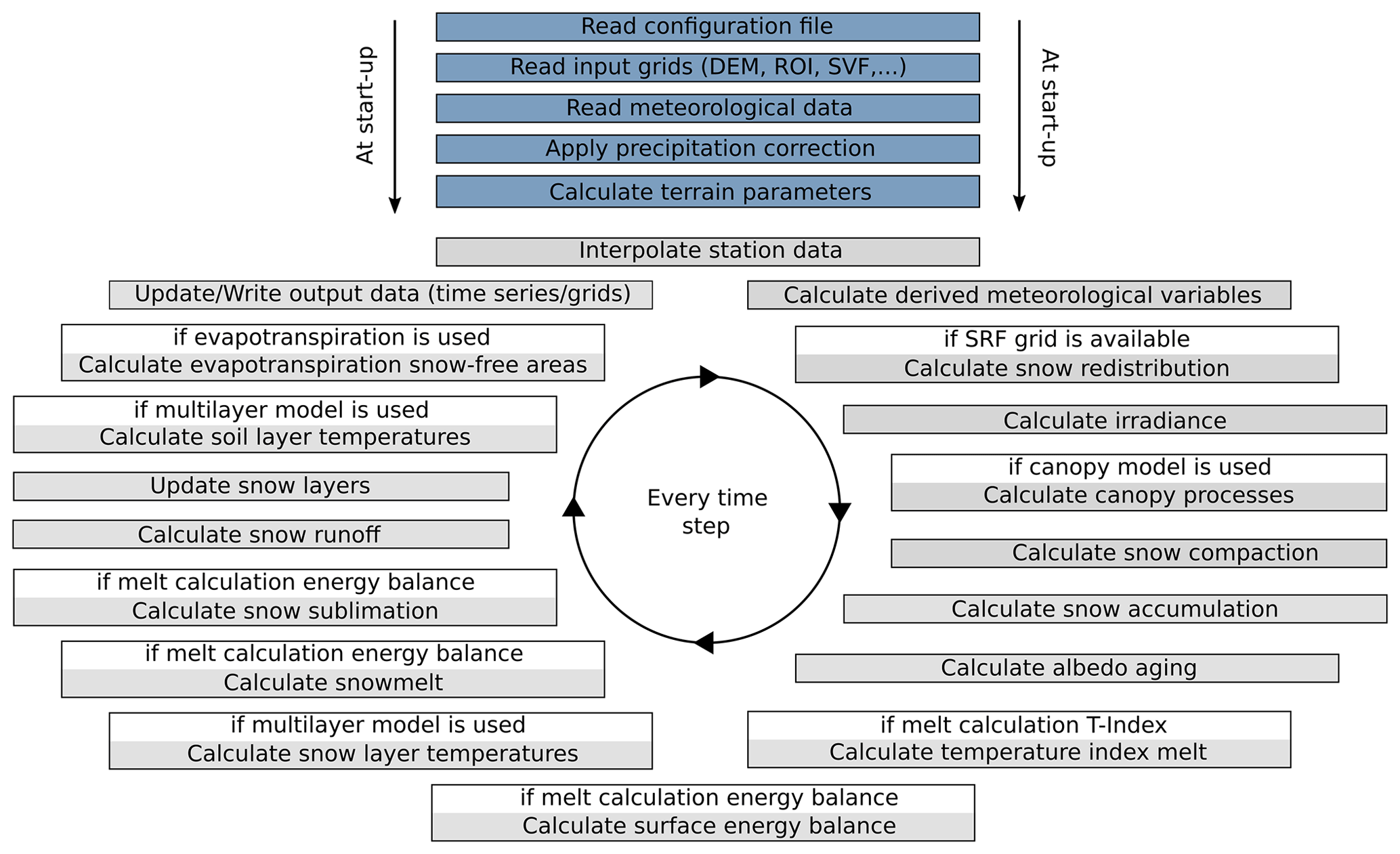
Figure 3 Flowchart showing the repetitive circle of a typical openAMUNDSEN model run. The reading of the input is succeeded by the computation of several precipitation correction and terrain parameters. After that, the loop for all time steps of the model run is entered.

3.2 Temporal and spatial discretization

Usually, the model is driven with a temporal resolution that is in accordance with the one of the used meteorological-forcing variables. For model applications which require a higher temporal resolution (or if only daily recordings are available), methods exist to disaggregate the measurements accordingly (e.g., MELODIST; Förster et al., 2016). For simulations with a lower temporal resolution than the forcing, aggregation is done during runtime. The output temporal resolution can be any aggregate of the original computation resolution – usually daily, monthly, and yearly. All of this is arbitrarily set in the model configuration prior to the model run. The minimum spatial resolution is not limited. Theoretically, a 1 m or even higher resolution (e.g., laser-scan-derived) DEM can be used as basis for the model simulation. A comparatively high resolution is thereby beneficial for adequately capturing all small-scale processes shaping the snow cover distribution in complex terrain. However, it is questionable whether such computational effort is meaningful with respect to the availability and quality of the forcing data and in relation to the scale of the considered processes. According to our experiences from typical mountain catchments in the European Alps, a resolution between 10 and 1000 m is often a good compromise between detail representation and computational efficiency. The size of the modeled domain can be anything between one single pixel and some thousands of square kilometers (see Fig. 1a). De Gregorio et al. (2019a, b), for example, successfully applied the model for the Euregio Tyrol–South Tyrol–Trentino (Austria–Italy), which has a size of 26 254 km².

3.3 Spatial interpolation of meteorological measurements

openAMUNDSEN includes a meteorological pre-processor for the spatial interpolation of scattered point measurements, irrespective of whether these are provided irregularly (weather station recordings) or arranged as a regular grid (raster stack of weather or climate model output). In the latter case, the meteorological variables are resampled to grids with the given DEM spatial resolution. The minimum forcing required by the model consists of recordings of temperature and precipitation (when running in temperature index mode). For energy balance calculations, relative humidity, global radiation (or cloudiness), and wind speed are required in addition. If meteorological time series from station recordings are used as input, the model interpolates the measurements from their geographical locations to each grid cell inside the ROI (Fig. 4). In most simulation cases, recordings of the meteorological variables for the 2 m observation level are available. The distance between a variable snow surface and the sensor height can therefore be corrected in the modeling. To spatially interpolate the station observations in each model time step, the following IDW-based interpolation procedure is applied:

• A regression analysis between observations and the associated station elevation is performed to derive an elevation-dependent trend function, namely the lapse rate (LR).

• The derived function is applied to all cells of the DEM to create an elevation trend field for each meteorological variable, the “regression field” (Fig. 4a and d).

• The residuals for all station locations are calculated by subtracting the calculated regression value for the station elevation from the actual measurement at the station location for the current time step.

• The residuals for the station locations are interpolated to the grid using an IDW method, resulting in the “residual field” (Fig. 4b and e).

• This interpolated residual field is added to the regression field, which results in elevation- and station-distance-dependent interpolated fields for all meteorological variables (Fig. 4c and f).

Figure 4 exemplarily shows the steps of this IDW-based interpolation procedure for temperature and precipitation. It can be seen that, for both meteorological variables, a dependency of the recordings on elevation does exist (Fig. 4a and d), but, locally, some deviations of the measurements from the elevation trend occur (Fig. 4b and e). In the result, both patterns are visible. The procedure automatically fills potential gaps in the observation time series at the weather station locations. If only one observation for the LR determination exists at a given time step for the entire domain, this one observed value is uniformly distributed over the domain.

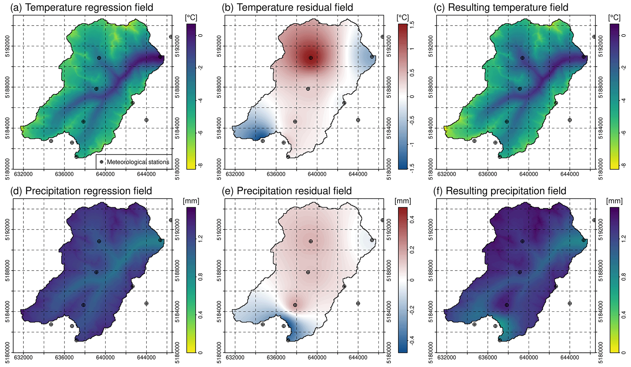
Figure 4 Regression field; residual field; and the resulting meteorological field, i.e., sum of the two for the spatial interpolation of meteorological variables in each single time step, exemplarily shown for temperature (a, b, c) and for precipitation (d, e, f) on 24 December 2019 at 10:00 LT (local time, UTC+1) for the Rofental. The resolution of the interpolated grid is 20 m.

Instead of the dynamic LR calculated from the local observations in each time step, the prescribed average monthly values of MicroMet (Liston and Elder, 2006) can be used. MicroMet is a quasi-physically based meteorological observation distribution system of intermediate complexity that produces high-resolution atmospheric forcings required to run spatially distributed terrestrial models in complex topography. It distributes the variables of air temperature, relative humidity, wind speed, incoming solar (shortwave) and longwave radiation, surface pressure, and precipitation following a Barnes objective analysis scheme (Barnes, 1964), similarly to the IDW procedure applied in openAMUNDSEN. A detailed comparison of results achieved with the interpolation schemes of openAMUNDSEN and MicroMet (and others, e.g., MeteoIO; Bavay and Egger, 2014) and their respective effects on the modeling of snow processes would be an interesting task of scientific value, but this is beyond the scope of this paper. Here, we only demonstrate the dynamic (mostly hourly) derived from the station observations in openAMUNDSEN for the Rofental and their monthly averages compared to the standard temperature LR and the monthly values originating from other regional contexts (Fig. 5): e.g., the monthly average temperature LRs derived for the Upper Danube catchment in central Europe are several degrees above the ones derived for the Northern Hemisphere; this shows the necessity of calculating LR using local observations. It should be noted, however, that dynamic temperature LRs and their monthly averages may vary from year to year.

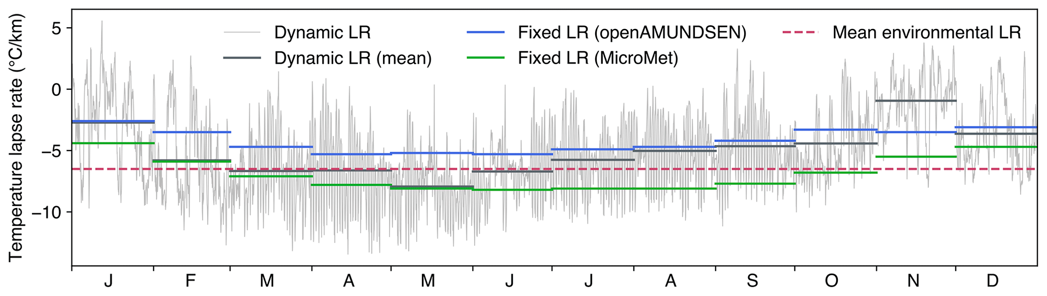
Figure 5 Dynamic (mostly hourly) temperature LR for 2020 in the Rofental (gray). The fixed LRs are monthly averages derived for the Upper Danube catchment (blue; Marke, 2008) and the Northern Hemisphere (green; Liston and Elder, 2006). The dashed line shows the mean environmental LR of −6.5 °C km⁻¹. Monthly averages computed for the dynamic LR (derived from the observations in each model time step) are dark gray.

Finally, the precipitation phase is determined in openAMUNDSEN by either air temperature or wet-bulb temperature thresholds (wet-bulb temperature is computed by iteratively solving the psychrometric equation). For both methods, a temperature transition range is defined. Above this transition range, precipitation is determined to be liquid, and it is determined to be solid below the lower end of the temperature range. Within the defined temperature range, the fractions of solid and liquid precipitation are linearly distributed between 100 % liquid at the upper end of the range and 100 % solid at the lower end of the range, with a 50 % liquid–solid fraction of precipitation at the threshold temperature. The threshold used in the presented simulations was chosen empirically: a value of 0.5 °C wet-bulb temperature with a transition extent from 0 to 1 °C produced reliable results in many numerical experiments with the model, in particular for the well-gauged site of Rofental (see Hanzer et al., 2016).

3.4 Radiative fluxes

Incoming global radiation strongly varies in time and space depending on terrain characteristics, the position of the sun, and atmospheric conditions. Hence, openAMUNDSEN calculates potential global radiation for each grid cell based on local aspect and slope, the position of the sun, orographic shadows, atmospheric transmission losses and gains due to scattering, absorption and reflections, multiple reflections between snow and clouds, and reflected radiation from snow-covered neighboring slopes. Cloud coverage (when not prescribed) is either determined by comparing potential to observed global radiation or, alternatively, estimated using atmospheric humidity following Liston and Elder (2006). During the nighttime, either the atmospheric-humidity approach is used or cloudiness is kept constant. In the final step, cloud coverage is spatially interpolated, and actual incoming global radiation is calculated by correcting potential global radiation with cloud coverage for each model grid cell.

Reflected shortwave radiation depends on surface albedo, which strongly varies in space and time, for snow surfaces that are mainly dependent on grain size. In openAMUNDSEN, albedo is modeled by taking into account snow age and an air-temperature-dependent decay function following Rohrer (1992) and Essery et al. (2013):

$$\begin{array}{}\text{(1)}& \mathit{\alpha }={\mathit{\alpha }}_{\min }+\left({\mathit{\alpha }}_{t-\mathrm{1}}-{\mathit{\alpha }}_{\min }\right)\cdot e^{-\frac{\mathrm{1}}{\mathit{\tau }}\mathit{\delta }t},\end{array}$$

where α_min is the (prescribed) minimum albedo, α_t−1 is the albedo in the previous time step, δt is the time step length, and τ is a temperature-dependent recession factor (implemented by prescribing two factors τ_pos and τ_neg for positive and negative air or, optionally, surface temperatures). Maximum snow albedo α_max is, by default, set to 0.85, while α_min, τ_pos, and τ_neg are set to 0.55, 200 h, and 480 h. Firn and ice albedo are held constant with α_firn=0.4 and α_ice=0.2 by default. Fresh snow increases albedo, either using a step function – increasing albedo to α_max when a snowfall above a certain threshold amount per time step (default: 0.5 kg m⁻² h⁻¹) occurs – or using the continuous function

$$\begin{array}{}\text{(2)}& \mathit{\alpha }={\mathit{\alpha }}_{t-\mathrm{1}}+\left({\mathit{\alpha }}_{\max }-{\mathit{\alpha }}_{t-\mathrm{1}}\right){\displaystyle \frac{S_{\mathrm{f}}}{S_{\mathrm{0}}}},\end{array}$$

where S_f is the snowfall amount, and S₀ is the snowfall required to refresh albedo (Essery et al., 2013).

Incoming longwave radiation from the atmosphere is a function of atmospheric conditions and temperature and is determined using the Stefan–Boltzmann law. Atmospheric emissivity thereby depends on water vapor content in clear-sky conditions and on cloud cover in overcast situations. Additionally, openAMUNDSEN accounts for longwave radiation from the neighboring slopes. Outgoing longwave radiation is calculated following the Stefan–Boltzmann law with the emissivity of snow and modeled snow surface temperature. The details of the radiation model mostly follow Corripio (2003) and are described in Strasser et al. (2004).

3.5 Precipitation correction

Precipitation measurements are vital input for every snow-hydrological model. However, measuring solid precipitation in complex alpine terrain is prone to large errors, which typically results in an undercatch of precipitation (Rasmussen et al., 2012). This is particularly important for mountain regions with a high amount of solid precipitation. High wind speeds can cause an undercatch of snowfall of up to 50 % (Kochendorfer et al., 2017) when using typical pluviometers of the Hellmann type. For solid precipitation, different correction methods are implemented in the model in order to account for the undercatch of precipitation gauges when measuring snow accumulation. Hanzer et al. (2016) showed that a combination of a weather-station-based snow correction factor taking into account wind speed and air temperature based on an approach by the World Meteorological Organization (WMO; Goodison et al., 1998) with a subsequent constant post-interpolation additional factor yielded plausible precipitation amounts. While the first correction is applied for the station recording amount prior to interpolation to the cells of the rectangular grid, the latter is added to all grid cells of the modeling domain. As an alternative to the WMO approach, a method which estimates undercatch regardless of precipitation phase (Kochendorfer et al., 2017) can be selected in the model configuration procedure prior to a model run.

3.6 Snow redistribution

Irrespective of whether there is rain or snow, with the IDW interpolation scheme in openAMUNDSEN, the amount of precipitation is distributed over the domain depending on the grid cell elevation, the distance of the surrounding weather stations, and the selected gauge undercatch correction method. The amount of observed snow at a certain location, however, can be significantly affected by the lateral processes of preferential deposition, erosion, and lateral redistribution. These processes are driven by wind and gravitational forces (Warscher et al., 2013; Grünewald et al., 2014). Many approaches with different levels of complexity exist to account for these processes; a recent and comprehensive overview of modeling lateral snow redistribution is given by Quéno et al. (2024). Such a consideration of the lateral snow redistribution processes is required to prevent artifacts of continuous snow accumulation on high summits and crests in long-term simulations where melt during summer is not sufficient to remove the amount of snow accumulated during the previous winter. The result will be that, with an increasing simulation period, in such locations, “snow towers” will continuously grow, whereas, in depressions beneath, snow accumulation will be underestimated (Freudiger et al., 2017). As a consequence, the mass balances of existing glaciers in such locations will be increasingly wrong due to not enough mass being deposited in the accumulation areas. Mass balances therefore are a useful measure to evaluate the simulations with respect to the lateral snow redistribution processes, as demonstrated by Hanzer et al. (2016). In openAMUNDSEN, a snow redistribution factor (SRF) field can be used to parameterize spatial snow distribution. The SRF describes the fractional amount of snow that is either eroded or deposited at each pixel location and modifies the interpolated snowfall field accordingly. Since SRF derivation can depend on various topographic parameters such as elevation, slope, aspect, curvature, viewshed, or terrain roughness and generally requires site-specific calibration (Grünewald et al., 2013), openAMUNDSEN allows for flexibility in calculating the SRF field. It provides functions to compute these topographic parameters but does not prescribe a singular method for final SRF calculation. Instead, the user of the model can decide in which way the snow redistribution should be parameterized in the model and if and how the results of the selected method should be calibrated and evaluated.

In the presented application for the Rofental, the concept of negative topographic openness (Yokoyama et al., 2002) has been used to parameterize spatial snow distribution. It is obtained by averaging the nadir angles calculated for all eight compass directions from the grid point, yielding low values for convex topographic features and high values for concave topographic features. The openness values finally depend on a length scale which describes the spatial dimension of the given topographic features affecting the redistribution processes, resulting in a snow redistribution factor which describes the fractional amount of snow eroded or deposited for any pixel location. The length scale depends on the shape and size of the topographic features of a landscape and the spatial resolution of the used DEM, and it should therefore be determined for each modeling domain and model application separately. For the example presented here, it has been empirically determined for the area of the Ötztal Alps (Austria) by Helfricht (2014). Effectively, the SRF approach as parameterized in openAMUNDSEN takes into account the processes of preferential deposition, wind-induced erosion, saltation, and turbulent suspension of atmospheric (snow) precipitation. The way it is implemented in the model, however, does not account for single events of lateral snow redistribution but rather accounts for their accumulated effect over longer simulation periods. Figure 6 shows an example of a snow redistribution factor field calculated using a combination of negative openness fields using two different length scales L (Hanzer et al., 2016): negative openness was calculated for the entire Ötztal mountain range based on a 50 m DEM for L=50 m and L=5000 m. While the smaller value accounts for small-scale topographic features with a high spatial variability, with the higher value, the large-scale topographies of ridges and valley floors are considered; hence, we see the overdeepening of the surface elevation of glacier tongues compared to the surrounding ridges and peaks (Helfricht, 2014). Details of the computation are given in Hanzer et al. (2016). Results show the (red) areas of the summits and ridges where snowfall is significantly reduced, whereas, in the slopes and valley bottoms, it is subsequently accumulated (blue areas; Fig. 6a). Correspondingly, in the presented example, the respective exposed areas received much less precipitation in May 2018 than the slopes and down-valley areas (Fig. 6b).

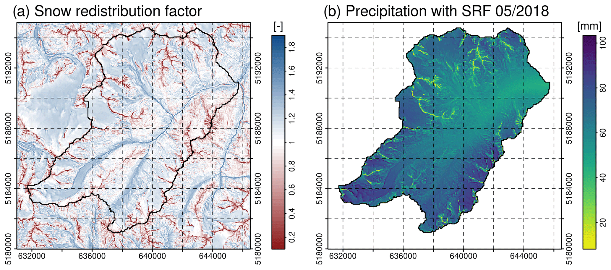
Figure 6 The snow redistribution factor (SRF) used in openAMUNDSEN to compensate for snow erosion on exposed ridges and for snow deposition in the slopes and depressions beneath (a) and an example of monthly total precipitation with lateral redistribution of snowfall (for May 2018), determined with the snow redistribution factor (b).

Together, three snow amount corrections can be applied in openAMUNDSEN: (i) a wind-speed- and temperature-dependent precipitation correction at the site of the measurement, (ii) an additional post-interpolation factor (see Sect. 3.5 for a description of how this is modeled), and (iii) the presented adjustment accounting for lateral snow redistribution. While (i) and (ii) increase the amount of measured precipitation towards a more realistic volume over the entire grid, (iii) solely redistributes the solid amount of precipitation from areas of erosion to areas of deposition.

3.7 Snow–canopy interaction

Forest canopies generally lead to a reduction in global radiation, precipitation, and wind speed at the ground, whereas humidity and longwave radiation are increased, and the diurnal temperature cycle is dampened. In openAMUNDSEN, the micrometeorological conditions for the ground beneath a forest canopy are derived from the interpolated measurements (assuming the weather stations are located in the open) by applying a set of modifications for these meteorological variables. The modifications are based on the effective leaf area index of the trees composing the stands, i.e., the sum of the classical LAI and the cortex area index (CAI) (Strasser et al., 2011). By means of the modified meteorological variables, the processes of interception, sublimation, unloading by melt, and fall-down as a result of exceeding the canopy snow-holding capacity are calculated. Liquid precipitation is assumed to fall through the canopy and is added to the ground snow cover (see Fig. 1d).

Simulations with the snow–canopy interaction model for an idealized mountain (Strasser et al., 2011) showed that, despite reduced accumulation of snow on the ground beneath the trees, both the rates and seasonal totals of the sublimation of snow previously intercepted in a canopy were significantly higher than the sublimation losses from the ground snow surface. On top of that, shadowing leads to reduced radiative energy input inside the canopy and hence to protection of the snow on the ground. The type of forest, exposition, the specific meteorological conditions, and the general evolution of the winter season play important roles as well: during winter, the effect of reduced accumulation is dominant, whereas, during spring, the shadowing effect with reduced ablation prevails. In winters with much snow, the effect of shadowing by the trees dominates, and snow lasts longer inside the forest than in the open. In winters with little snow, however, the sublimation losses of snow are dominant, and the snow lasts longer in open areas. This might vary, however, for northern and southern exposure to radiation and with the time of the year due to the strong effect of solar radiation on melt. In early and high winter, the radiation protection effect of shadowing is small. An intermittent meltout of the snow cover beneath the trees can occur if little snow is available. The shadowing effect becomes more efficient, and snowmelt is delayed relative to non-forested areas in late winter and spring. Due to the combination of all these processes, the modeling of snow–canopy interaction can lead to complex and very heterogeneous patterns of snow coverage and duration in alpine regions with forest stands (Essery et al., 2009; Rutter et al., 2009; Strasser et al., 2011).

3.8 Crop evapotranspiration

For non-snow-covered surfaces, the actual evapotranspiration of vegetated areas is calculated using the Food and Agriculture Organisation (FAO) Penman–Monteith approach (Allen et al., 1998), for which a schematic overview is illustrated in Fig. 7. In a first step, the evapotranspiration is calculated for a reference crop (grass) using the meteorological variables and a limiting amount of available water in the soil storage. In forested areas, thereby, the inside-forest meteorological conditions are considered. Then, the resulting evapotranspiration is modified according to the vegetation type using particular crop coefficients which integrate the effects of plant height, albedo, stomata resistance, and exposed soil fraction. Crop coefficients are available for a wide range of plant types in the given literature and change their values seasonally according to predefined growth stage lengths. For each plant type, evapotranspiration can either be calculated using a single-coefficient approach which integrates the effects of crop transpiration and soil evaporation into a single coefficient or using a dual-coefficient approach which considers crop transpiration and soil evaporation separately. Soil evaporation is computed considering the cumulative depth of water evaporated from the topsoil layer and the fraction of the soil surface that is both exposed and wetted. The soil type thereby determines the amount of evaporable water with respect to field capacity, water content at wilting point, and depth of the surface soil layer that is subject to drying by means of evaporation (0.10 to 0.15 m); parameters are available for sand, loamy sand, sandy loam, loam, silt loam, silt, silty clay loam, silty clay, and clay (Allen et al., 1998). With this approach, the water balance of the upper soil layer is computed, determining if surface runoff and deep percolation can occur or if evapotranspiration is limited. If the evapotranspiration module is activated, both soil types and land cover must be available as rasterized maps in the DEM geometry.

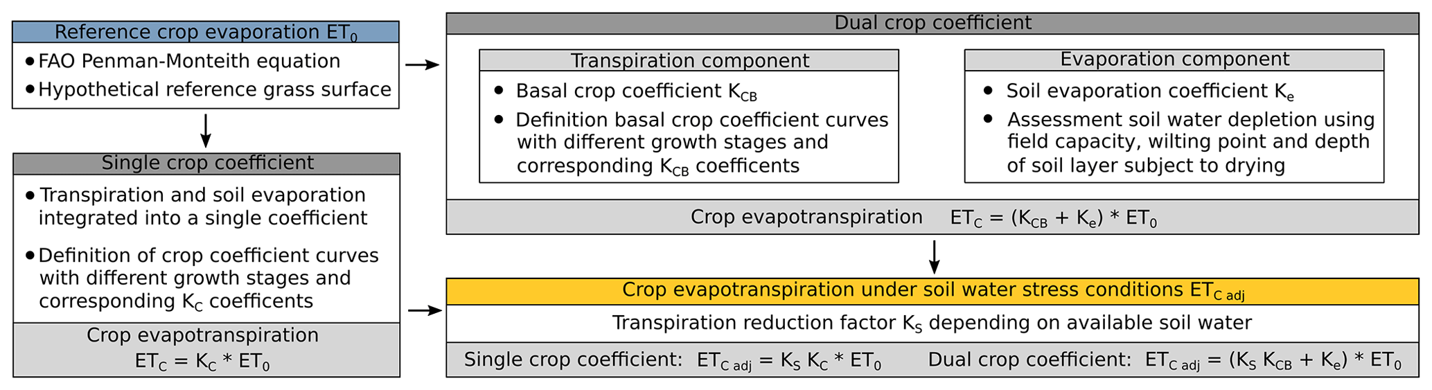
Figure 7 Schematic overview of the FAO evapotranspiration module to compute the water flux from the soil through the plants to the atmosphere with the Penman–Monteith equation. Fluxes are calculated for a reference crop and then scaled to other land use classes.

3.9 Layering schemes

In openAMUNDSEN, two different layering schemes for snow- or ice-covered surfaces are implemented (see Fig. 1c). The “cryospheric-layer version” parameterizes layers of new snow, old snow, firn, and glacier ice. The advantage of using these layers is that they are distinctively different in their optical properties, and, hence, their surfaces can be recognized and distinguished in the field, on photographs, or by satellites with sensors that are sensitive to the visible range of the electromagnetic spectrum. The model tracks the thickness of these layers and parameterizes their density with more-or-less-empirical relations. For the snow–soil interface, a fixed upward heat flux can be set (often 2 W m⁻² in the Alpine region). The most comprehensive descriptions of this model version can be found in Strasser (2008), Strasser et al. (2011), and Hanzer et al. (2016).

The “multilayer version” is adopted following the structure of the FSM model (Essery, 2015). It considers a number of layers (by default, three) with fixed maximum depths (for the upper two ones), all of them without physical representation. In this model version, the fluxes of mass and energy are tracked by means of an iterative computation of the state variables of temperature and liquid-water content such that the balances of mass and energy are closed for each layer. The energy transfer at the snow–soil interface is calculated by means of a four-layer soil model. A detailed description of the implemented multilayer model scheme can be found in Essery (2015).

Whereas the cryospheric-layer version of openAMUNDSEN can be combined with both the simple and the enhanced temperature index approach or, alternatively, with the energy balance method, the multilayer version requires the energy balance method to compute the energy and mass balances of the surface and the snow layers beneath. The simulation of glacier evolution as a response to the climatic conditions presupposes that the cryospheric-layer version is applied.

3.9.1 Cryospheric-layer version

In the cryospheric-layer version of openAMUNDSEN, the transitions between new snow and old snow occur when reaching a predefined snow density threshold (by default, 200 kg m⁻³), while remaining snow amounts at the end of the ablation season are transferred to the firn layer (by default, on 30 September). Compaction for the new- and old-snow layers is calculated using the methods described below (in Sect. 3.10); for firn, a linear densification is assumed. Once reaching a threshold density of 900 kg m⁻³, firn is added to the ice layer beneath. While snow albedo is parameterized using the aging-curve approach (Rohrer, 1992), firn and ice albedo are kept constant (with default values of 0.4 and 0.2, respectively). The details of the cryospheric-layer version of openAMUNDSEN are best described in Hanzer et al. (2016).

While snow temperature of the individual layers is not calculated using the cryospheric-layering scheme, an approach following Braun (1984) and Blöschl and Kirnbauer (1991) is applied in order to determine an average cold content of the snow layers. This cold content builds up when the snowpack cools; it has to be depleted before melt and subsequent runoff can occur at the snowpack bottom. The maximum possible cold content is thereby set to 5 % of the total snowpack weight (the latter can be converted to an energy by multiplication with the latent heat of fusion).

When using this scheme, the snowpack is taken as a bulk layer to solve the surface energy balance. If the air temperature is above 0 °C, the model assumes that the snow surface temperature is 0 °C and that melt occurs, the amount of which can be computed from the available excess of the energy balance. If the air temperature is below 0 °C, an iterative procedure to compute the snow surface temperature for closing the energy balance is applied. With this procedure, the snow surface temperature is altered until the residual energy balance passes zero.

3.10 Multilayer version

In the multilayer version of openAMUNDSEN, the vertical heat fluxes are computed both through the snowpack and into the ground (Essery, 2015). To solve the energy balance, melt is first assumed to be zero for the surface temperature change of every time step. Snow is considered to be melting if the energy balance results in a surface temperature passing 0 °C. The temperature increment is recalculated assuming that all of the snow melts; if this results in a surface temperature below 0 °C, snow only partially melts during the time step (Essery, 2015). Snow layer temperatures are then updated using an implicit finite-difference scheme. The snow compaction and density of each layer are calculated in the same way as for the cryospheric-layer version, as described in the following.

3.11 Snow density

For both layering schemes, fresh-snow density is calculated using the temperature-dependent parameterization by Anderson (1976), assuming a minimum density of 50 kg m⁻³. Snow compaction can be calculated using two methods, one physically based approach following Anderson (1976) and Jordan (1991), and one empirical approach following Essery (2015). For the former, density changes are calculated in two stages due to snow compaction and metamorphism, taking into account temperature and snow load imposed by the layers above (see also Koivusalo et al., 2001). For the empirical method, assumptions are made for the maximum density of snow below 0 °C and for melting conditions (default values: 300 kg m⁻³ for cold snow and 500 kg m⁻³ for melting snow). The timescale for compaction is an adjustable parameter (default value: 200 h). The increase in density for every time step is calculated as a fraction of the compaction timescale multiplied by the difference between maximum density and the density of the last time step (Essery, 2015).

3.12 Liquid-water content

Meltwater occurring at the snow surface is not immediately removed from the snowpack, but a certain liquid-water content (LWC) can be retained. Following either Braun (1984) or Essery (2015), the maximum LWC is defined as a mass fraction of SWE or as a fraction of pore volume that can be filled with liquid water (volumetric water content). If the maximum LWC is reached during snowmelt, runoff at the bottom of a snow layer occurs and drains into the snow layer underneath or – for the bottom snow layer – into the upper soil layer. In the case of a negative energy balance, this liquid water can refreeze.

3.13 Snowmelt

Snowmelt can be computed in openAMUNDSEN using several approaches with different complexity. The simplest method, the classical temperature index approach, is particularly suitable for regions where only daily recordings of temperature and precipitation are available. Melt M in millimeters per time step is thereby computed as follows:

$$\begin{array}{}\text{(3)}& M=\left\{\begin{array}{ll}\mathrm{DDF}\cdot T& T>T_{\mathrm{T}}\\ \mathrm{0}& T\le T_{\mathrm{T}}\end{array},\right.\end{array}$$

with DDF being the degree day factor (or melt coefficient) (in mm w.e. °C d⁻¹) and T being the mean daily temperature (in °C). T_T is the threshold temperature above which melt is assumed to occur (e.g., 1 °C). Low DDFs will be obtained for cold and dry areas, whereas high DDFs can be expected for warm and wet areas.

Second is a hybrid approach between the temperature index method and the energy balance, the so-called enhanced temperature index method by Pellicciotti et al. (2005). By including potential shortwave radiation and albedo, these computations can also be applied to meteorological variables in hourly time steps:

$$\begin{array}{}\text{(4)}& M=\left\{\begin{array}{ll}\mathrm{TF}\cdot T+\text{RF}\cdot \left(\mathrm{1}-\mathit{\alpha }\right)\cdot G& T>T_{\mathrm{T}}\\ \mathrm{0}& T\le T_{\mathrm{T}}\end{array},\right.\end{array}$$

where T is an hourly temperature (in °C), α is albedo, and G is potential incoming shortwave radiation (which is simulated as described in Sect. 3.4). TF and RF are two empirical coefficients, the temperature factor and the shortwave radiation factor (expressed in mm h⁻¹ °C⁻¹ and m² mm W⁻¹ h⁻¹). T_T is equal to 1 °C. When temperature is below T_T, no melt occurs.

Melt rates using either the cryospheric-layer or the multilayer version of openAMUNDSEN can also be computed using the surface energy balance equation:

$$\begin{array}{}\text{(5)}& Q+H+E+A+B+M=\mathrm{0},\end{array}$$

with Q being the shortwave and longwave radiation balance, H being the sensible heat flux, E being the latent heat flux, A being the advective energy supplied by solid or liquid precipitation, and B being the soil heat flux. M is the energy that is potentially available for melt. For a detailed description of the calculation of the individual energy fluxes, see Strasser (2008). A comparison of modeling results achieved with the different approaches is shown in Fig. 8. The temperature index approach delivers results which only show dependence on the temperature and the precipitation gradient but no pattern affected by different radiative energy inputs depending on slope and aspect (Fig. 8a). These computations can be performed with a daily time step; hence they are comparably fast and only require temperature and precipitation as meteorological input variables. Using the energy balance for computation of the accumulation and ablation processes at the snow surface and the cryospheric-layer version for the internal processes inside the snowpack leads to a significantly more differentiated pattern in the resulting snow distribution (Fig. 8b): the result clearly shows the effect of topography on the ablation pattern of the snow cover on this day. In Fig. 8c, the energy balance was combined with the multilayer version of the model and the application of the SRF to consider the lateral snow redistribution processes. Now, erosion from exposed summit and ridge areas can be detected, as well as additional accumulation in the slopes beneath. This complex pattern best matches the snow distribution as depicted in the fractional snow cover map derived from a Sentinel-2 image captured on the same day (Fig. 8d). The comparison of the simulation results achieved with increasingly sophisticated model versions shows that their plausibility clearly improves with a consideration of radiative energy supply (Fig. 8b) and lateral snow redistribution (Fig. 8c).

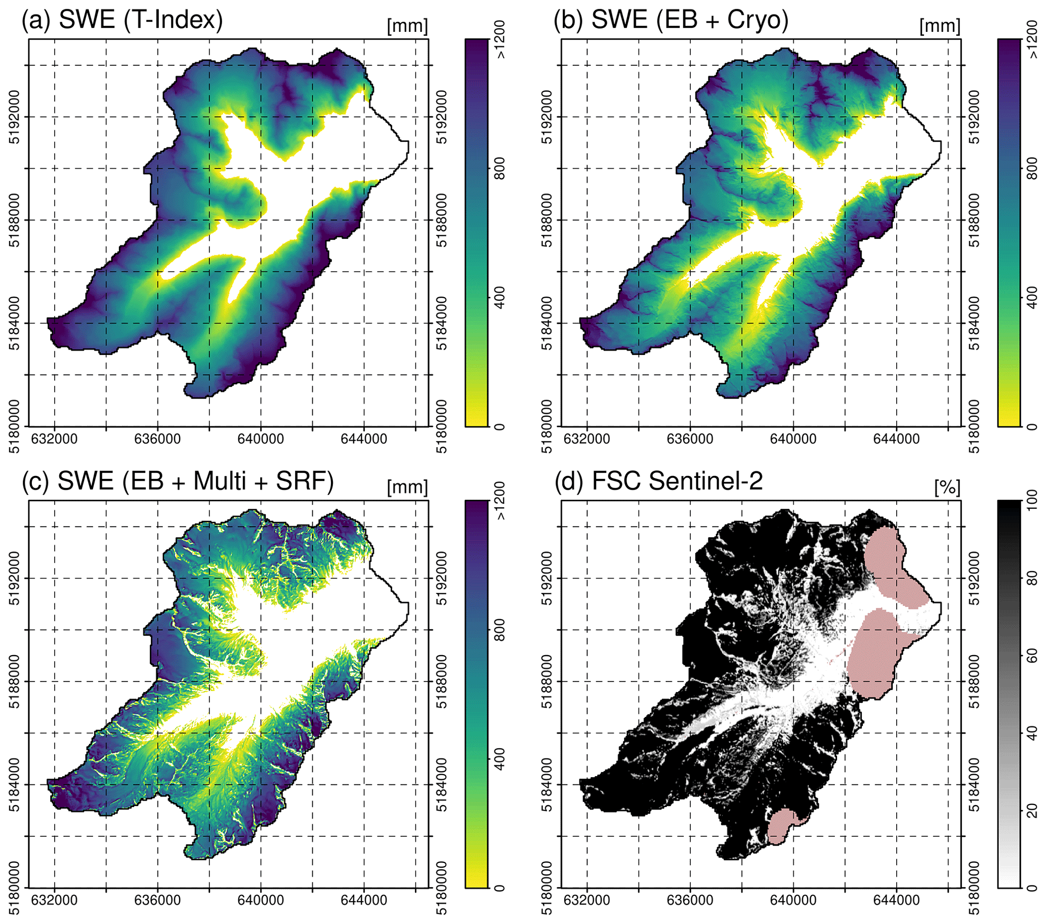
Figure 8 Snow water equivalent on 18 June 2019 in the Rofental, simulated using the temperature index approach at a daily resolution without wind-induced snow redistribution (a), using the energy balance (EB) approach and cryospheric layers (Cryo) without wind-induced snow redistribution (b) and using the energy balance (EB) approach with multiple layers (Multi) including wind-induced snow redistribution (SRF) (c). Panel (d) shows a fractional-snow-cover (FSC; including the glacier areas) map derived from Sentinel-2 satellite data for the same day (pink patches are unclassified pixels – in this case, clouds).

4 Implementation in Python

For the rewriting of the original AMUNDSEN IDL code, the Python language was chosen due to its popularity and simplicity and the large number of excellent and well-tested numerical and scientific libraries available. In particular, openAMUNDSEN makes use of the packages NumPy (Harris et al., 2020) for array calculations and pandas (McKinney, 2010) and Xarray (Hoyer and Hamman, 2017) for processing time series and multidimensional data sets. While Python, being a scripting language, has limitations in terms of execution performance, these libraries allow efficient code execution due to the use of Fortran or C for the underlying calculations. For increasing the runtime efficiency of performance-critical functions within openAMUNDSEN, the Numba library (Lam et al., 2015) is furthermore used for dynamically translating Python code into machine code.

openAMUNDSEN is implemented using an object-oriented architecture, centering around the OpenAmundsen class as the primary interface. This class represents a single model run and encapsulates all the methods required to initialize and run the model. openAMUNDSEN can either be used as a standalone utility (using the openamundsen command line tool) or as a Python library. When used in standalone mode, the openamundsen command line tool must be invoked with the name of a configuration file in YAML format (i.e., openamundsen config.yml). If used as a library from within a Python script, the model configuration in the form of a Python dictionary (again, commonly sourced from a YAML file) must be passed when instantiating an OpenAmundsen object. A typical model run executed from within Python looks as follows:

import openamundsen as oa

config = oa.read\textunderscore config('config.yml')
model = oa.OpenAmundsen(config)
model.initialize()
model.run()

This allows for substantial flexibility in simulation preparation, execution, and post-processing. For example, considering the following:

• It is possible to change the model state variables after initializing them (e.g., the snow layers – which are, by default, initialized as being snow-free – can be initialized using prepared snow depth or SWE data). This is not only possible prior to running the model but can also be done at any point during the model run by using model.run_single() – which performs the calculations for a single time step – in a loop instead of the model.run() call.

• Model results do not necessarily have to be written to file but can also be stored in-memory and accessed directly from the OpenAmundsen class instance for further processing.

• Several model runs can be prepared in a single script by initializing multiple OpenAmundsen instances and, e.g., being run in parallel.

Model runtime is influenced by various factors, most importantly the number of pixels simulated but also the number of weather stations used for interpolation of the meteorological variables, the choice of the layering scheme (cryospheric layers vs. multilayer), the activated submodules (snow–canopy interaction, evapotranspiration, etc.), the number of input–output (I–O) operations (the number of output variables and the temporal frequency at which they are written to file), and others. openAMUNDSEN generally leverages multiple CPU cores (by operating over the model grid pixels in parallel using Numba's parallelization features); however, in practice, the speedup gained by parallelism is small due to the short-lived nature of the respective functions and the overhead from scaling to multiple cores. To give an example, a point-scale (i.e., 1×1) model run completes a full-year simulation using hourly time steps in approximately 2 min on an AMD EPYC 7502P processor. A spatially distributed model run for a medium-sized model grid (450×650 pixels) requires approximately 36 min per simulation year in single-core mode and 33, 30, 28, and 27 min when using 2, 4, 8, and 16 cores, respectively. Running the model in pure Python mode (i.e., disabling the Numba just-in-time compilation) can increase runtime by a factor of more than 40.

5 Model uncertainty and evaluation

The original versions of ESCIMO and AMUNDSEN have been extensively validated in various alpine sites (Strasser and Mauser, 2001; Strasser et al., 2002; Strasser, 2004; Pellicciotti et al., 2005; Strasser et al., 2008; Strasser, 2008; Hanzer et al., 2014; Marke et al., 2015). Hanzer et al. (2016) showed the uncertainty of the model application by means of a systematic, independent, complete, and redundant validation procedure based on the observation scale of temporal and spatial support, spacing, and extent (Blöschl, 1999). To evaluate the dimensions of the observation scale, a comprehensive set of eight independent validation sources was used: (i) mean areal precipitation derived by conserving mass in the closure of the water balance, (ii) time series of snow depth recordings at the plot scale, (iii–iv) multitemporal snow extent maps derived from Landsat and MODIS satellite data products, (v) snow accumulation distribution derived from airborne-laser-scanning data, (vi) specific surface mass balances for three glaciers in the study area, (vii) spatially distributed glacier surface elevation changes for the entire area, and (viii) runoff recordings for several subcatchments. By means of this evaluation procedure, both the simulated spatial patterns of the snow cover and the time series of its evolution are quantitatively analyzed with a maximum of considered independent comparison measures; the method hence represents an unprecedented completeness in the comparison of the simulation results with observations. The results indicate an overall high model skill in all the dimensions and confirmed the very good model evaluations of the published case studies (Hanzer et al., 2016). As an example of the model performance at the location of a meteorological station, Fig. 9 shows snow depth (Fig. 9a) and SWE (Fig. 9b) simulation results achieved with meteorological observations at the Proviantdepot station (2737 m a.s.l.) compared to recordings of snow depth for the winter seasons of 2020–2021 and 2021–2022. All model versions capture well the seasonal course of the snow depth evolution. Of course, the temperature index version could be optimized by means of calibration to better match the meltout time; thus, the lag of some days is not a lack of model “accuracy” in this case (a standard degree day factor of 6.0 mm K⁻¹ d⁻¹ was used, the same as for the results in Fig. 8a, without further calibration). The energy balance version of the model using the multilayer approach and considering lateral snow redistribution provides the best-matching representation of the observations.

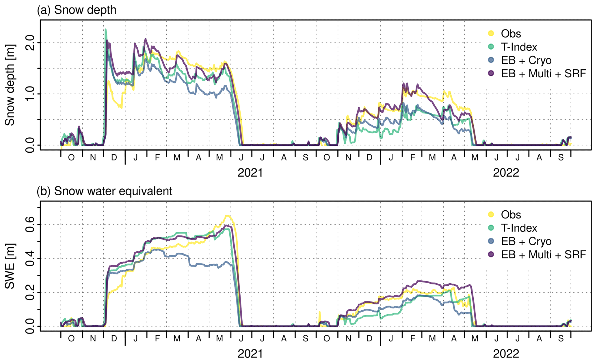
Figure 9 Observed and simulated snow depth (a) and SWE (b) at the location of the meteorological station Proviantdepot (2737 m a.s.l.), located in the area of the example application of Rofental (46.82951° N, 10.82407° E) for the winter seasons of 2020–2021 and 2021–2022. The Pearson correlation, Nash–Sutcliffe efficiency, Kling–Gupta efficiency, and RMSE for the T-index simulations of snow depth are 0.92, 0.79, 0.77, and 0.269, and for SWE, they are 0.96, 0.93, 0.94, and 0.055. For the EB + Cryo model version, they are 0.93, 0.70, 0.61, and 0.283 (snow depth) and 0.94, 0.76, 0.65, and 0.076 (SWE), and for the EB + Multi + SRF model simulation, they are 0.96, 0.92, 0.95, and 0.186 (snow depth) and 0.98, 0.95, 0.88, and 0.046 (SWE).

For the multilayer version of the openAMUNDSEN model, the uncertainty of the model simulations was investigated by Günther et al. (2019) for point simulations at the local scale and by Günther et al. (2020) for distributed applications.

openAMUNDSEN was also subject to several model intercomparison studies. The very first version of the bulk energy balance approach of AMUNDSEN (then still called ESCIMO) was compared to CROCUS for data of the Col de Porte weather station located in the French Alps (1340 m a.s.l.) (Strasser et al., 2002). Later, the model was intercompared to many other snow models in the series of the international Snow Model Intercomparison Projects (SnowMIPs): in the original SnowMIP project (Etchevers et al., 2004), ESCIMO was evaluated together with 22 other snow models of varying complexity at the point scale using meteorological observations from the two mountainous alpine sites of Col de Porte (1340 m a.s.l.) and Weissfluhjoch (2540 m a.s.l.), both in the European Alps. In the follow-up project SnowMIP2 (https://www.geos.ed.ac.uk/~ressery/SnowMIP2.html, last access: 1 June 2024), 33 snowpack models of varying complexity and purpose were evaluated across a wide range of hydrometeorological and forest canopy conditions at five Northern Hemisphere locations, namely (Essery et al., 2009; Rutter et al., 2009) Alptal (Switzerland; 1185 m a.s.l.), BERMS (Canada; 579 m a.s.l.), Fraser (USA; 2820 m a.s.l.), Hitsujigaoka (Japan; 182 m a.s.l.), and Hyytiälä (Finland; 181 m a.s.l.). For each location, two sites were used, one in the open (no canopy) and one forested (canopy) site. Finally, the surface energy balance core of the model participated in ESM-SnowMIP (https://climate-cryosphere.org/esm-snowmip/, last access: 1 June 2024), an international intercomparison project to evaluate 27 current snow models against local and global observations for a wide variety of settings, including snow schemes that are included in Earth system models (Krinner et al., 2018). A further objective of ESM-SnowMIP was to better quantify snow-related feedbacks in the Earth system. ESM-SnowMIP is tightly linked to the Land Surface, Snow and Soil Moisture Model Intercomparison Project (https://climate-cryosphere.org/ls3mip/, last access: 1 June 2024), which is a contribution to the sixth phase of the Coupled Model Intercomparison Project (CMIP6; https://wcrp-cmip.org/cmip-phase-6-cmip6/, last access: 1 June 2024). One of the results of ESM-SnowMIP was an unexpected surprise, specifically that more sites, more years, and more variables do not necessarily provide more insight into key snow processes; instead, “this led to the same conclusions as previous MIPs: albedo is still a major source of uncertainty, surface exchange parameterizations are still problematic, and individual model performance is inconsistent. In fact, models are less classifiable with results from more sites, years, and evaluation variables” (Menard et al., 2021). Currently, openAMUNDSEN belongs to the range of models within the COPE initiative (Common Observing Period Experiment) of the INARCH project (https://inarch.usask.ca/science-basins/cope.php, last access: 1 June 2024). It can be expected that many new insights about the models internals will mutually be learned from these model intercomparisons in the upcoming future.

6 Conclusions

In this paper, we present openAMUNDSEN, a fully distributed open-source snow-hydrological model for mountain catchments. The model includes a wide range of process representations of an empirical, semi-empirical, and physical nature. openAMUNDSEN allows finding a compromise between temporal and spatial resolutions, the time span of the simulation experiment, the size of the considered region, physical detail and consistency, and performance. For example, it offers choices between the temperature index approach to determine snowmelt rates from daily temperature and precipitation or hourly closure of the surface energy balance and the calculation of a number of state variables for several snow layers using temperature, precipitation, humidity, radiation, and wind speed as forcing data. openAMUNDSEN is computationally efficient, of a modular nature, and easily extendible and also allows for using factorial designs to determine interactions between processes and their effect on the accuracy of the simulation results (Essery et al., 2013; Günther et al., 2019, 2020). Hence, the application of the model is very flexible, and it supports a multitude of applications or simulation experiments to address any kind of hydrological, glaciological, climatological, or related research questions.

The model has been evaluated and proven its applicability at many sites worldwide. Most of all, it was subject to a systematic, innovative, multilevel spatiotemporal validation with independent data sets of various resolutions and extents at an instrumented site in the European Alps (Hanzer et al., 2016). In all cases, the model showed high overall skill and captured well the spatial and temporal patterns and the magnitudes of the observations.

The Python model code for openAMUNDSEN is available for the public as an open-source project on GitHub (https://github.com/openamundsen/openamundsen, last access: 1 June 2024), including documentation which is subject to continuous extension and improvement (https://doc.openamundsen.org, last access: 1 June 2024). The bootstrap-resampling weather generator (see Appendix A) is available at https://github.com/openamundsen/openamundsen-climategenerator (last access: 1 June 2024).

7 Future developments

The openAMUNDSEN model code is being continuously further improved and extended. The modeling of the processes of lateral snow redistribution will benefit from a simulation of local wind fields, e.g., as recently demonstrated by Quéno et al. (2024). On top of the wind-induced processes of saltation, turbulent-suspension (with sublimation) snow is also transported downslope by means of avalanches, which is also the origin of accumulated masses of snow leewards of crests. In the original, IDL-based version of AMUNDSEN (Strasser, 2008), the avalanche process was parameterized based on the Mflow-TD algorithm by Gruber (2007); the latter was later extended with a continuous update of the surface elevation model to correct for eroded and/or deposited masses of snow (Bernhardt and Schulz, 2010). A comparable algorithm is in development and is to be included in openAMUNDSEN soon. Another path of improvement is foreseen for the snow–canopy interaction module. On the one hand, the parameterization of inside-canopy meteorological variables derived from measurements taken in the open will be further improved by utilizing the new (winter) measurements of inside-canopy meteorological variables, i.e., from the Col de Porte meteorological station in the French Alps (Sicart et al., 2023). Further, it is intended that the snow–canopy interaction module will be coupled with a dynamically simulated evolution of the LAI from iLand model simulations (Seidl et al., 2012). The ultimate goal of this effort is to bi-directionally couple the snow processes inside the canopy with its long-term evolution to enable the simulation of scenarios of the effect of climate change on the coupled hydrological–biological system of mountain forests.

To compute streamflow discharge in mostly glacierized catchments to be compared to gauge recordings, a linear-reservoir cascade approach following Asztalos et al. (2007) has been implemented as a separate post-processing tool (Hanzer et al., 2016). The linear-reservoir approach is a comparable simple empirical method to produce a runoff curve for a certain location of the stream without the need to provide physical parameters for the catchment characteristics (e.g., soil) or the wave propagation along the channel. Instead, a series of parallel linear-reservoir cascades (Nash, 1960) is computed, the parameters of which are calibrated by maximizing the Nash–Sutcliffe efficiency (NSE) and minimizing the relative volume error (following Lindström, 1997). Due to its purely empirical nature and the fact that its application is limited to small glacierized catchments with short concentration times only, the linear reservoir approach will not be included in the openAMUNDSEN project on the openAMUNDSEN GitHub repository. Instead, it is foreseen that new approaches in machine learning will be tested and developed, e.g., in the field of LSTM (long short-term memory network modeling), which can provide very good results for hydrological streamflow simulations (Kratzert et al., 2021). Other such new developments also exist in the combination of hydrological modeling, remote sensing, and machine learning (De Gregorio et al., 2019a, b). Since AI is a field of rapid development in scientific modeling, we also expect significant advances in snow-hydrological modeling using these innovative methods.

Finally, we see a promising way to increase the model accuracy by assimilating satellite-data-derived maps of, e.g., snow coverage and/or wet snow area to select the best-matching model run out of an ensemble of simulations that has been created by perturbating the meteorological forcing or the parameters of the model. First developments are already being undertaken in this direction. This way, the model can also be accurately initialized when applied for predictions using weather forecast model output as meteorological forcing.

Appendix A: Generation of potential future climate in openAMUNDSEN

Data time series of future climate evolution used to force openAMUNDSEN for climate change scenario simulations can be produced by means of a stochastic block bootstrap resampler, which is realized as an external pre-processing routine (https://github.com/openamundsen/openamundsen-climategenerator, last access: 1 June 2024). The method requires a sufficiently long time series of historical meteorological recordings from a period with as many as possible variable weather conditions in the considered region. The principles of the implemented weather generator follow Strasser (2008) and are described herein. A basic assumption of the method is that a climate storyline can be divided into time periods which are characterized by a certain mean temperature and precipitation and that these two variables are not independent from each other:

$$\begin{array}{}\text{(A1)}& P_{\mathrm{tot}}=f\left(T_{\mathrm{mean}}\right).\end{array}$$

Thereby, P_tot is the total precipitation amount of a specific time period, T_mean is the mean temperature, and f is their functional dependency. The time periods can be set to any length, i.e., to months as in Mauser et al. (2007) or to weeks as in Strasser (2008). In a first step, the typical annual course of the measured meteorological variables is constructed by computing mean temperature and total precipitation for the periods using all years of the historical data set and applying the given formula. While temperature is characterized by a typical seasonal course in the Alpine region (warm in summer, cold in winter), the annual course of the precipitation totals of a period of a certain duration can be more complex. The resulting mean annual climate course is used to construct the future data time series period by period: firstly, the respective temperature for the period is modified with a random variation factor and an assumed projected temporal trend (e.g., as derived from a regional climate model application). Then a corresponding precipitation is derived, along with, again, a random variation. In the end, the climate of a future period is defined by the obtained mean temperature and precipitation. In a final step, the period from the historical pool that has the most similar temperature and precipitation is selected by applying an Euclidian nearest-neighbor distance measure. All respective data of the chosen period (e.g., air temperature, precipitation, global radiation, relative humidity, and wind speed) are then added to the future time series to be constructed. This procedure is continuously repeated for all periods of the year and for all years of the future time series. By modifying the applied random variation, a change in climate variability can be simulated. To allow for more flexibility in the construction of the periods, in our implementation, the basic population from which the measured period is chosen (based on the number of periods available and being equal to the number of years for which observational data are available) can be synthetically extended by allowing for one or more periods before and after the one to be constructed (Fig. A1).

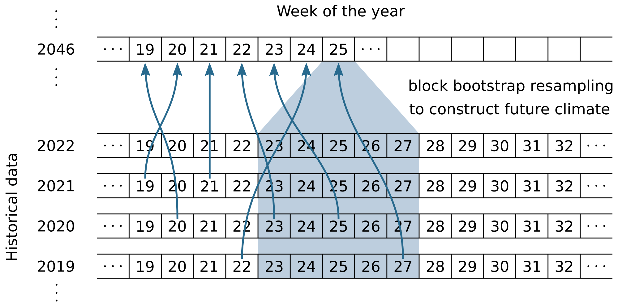
Figure A1 openAMUNDSEN pre-processing with the weather generator: choice of corresponding historical periods to construct a data time series of future climate evolution with preset trends and random variations from given meteorological observations. The number of periods from which data can be selected to construct a particular period of a year in the future time series is set to five in this example.

The described procedure has a number of specific features: (i) the key advantage of the method is that the physical relationship between the meteorological variables is maintained in the simulation; (ii) bootstrap models, such as the described one, obviously work well at a high temporal resolution, e.g., 1 to 3 hourly; (iii) the produced data time series is in the validated range for the subsequent hydrological modeling; (iv) a synthetic baseline scenario can easily be constructed by assuming a zero trend for temperature; (v) the procedure is computationally very efficient; and, finally, (vii) the spatial resolution of the data is preserved as it corresponds exactly to the weather station locations. However, a significant drawback of the method is that auto-correlation between the periods is lost, and the consideration of changes in the variability of the meteorological variables is limited. Together with the fact that changes in extreme values are not considered (only their frequency can change), it becomes clear that the data resulting from the method cannot be used for modeling variations in the extent of hydrological extremes. Furthermore, and most crucially, no coupling is considered between the (simulated) characteristics of the land surface – e.g., whether it is snow-covered or not – and the atmosphere; therefore, the important effects of feedback mechanisms are not conserved in the construction of the data time series. This, however, is a drawback that many physical climate models also share. Examples of the application of the procedure to the high Alpine region of the Berchtesgaden Alps (Germany) with subsequent modeling of snow processes, including snow–canopy interactions, are given in Strasser (2008).