Physics-motivated cell-octree adaptive mesh refinement in the Vlasiator 5.3 global hybrid-Vlasov code

Automatically adaptive grid resolution is a common way of improving simulation accuracy while keeping computational efficiency at a manageable level. In space physics, adaptive grid strategies are especially useful as simulation volumes are extreme, while the most accurate physical description is based on electron dynamics and hence requires very small grid cells and time steps. Therefore, many past global simulations encompassing, for example, near-Earth space have made tradeoffs in terms of the physical description and laws of magnetohydrodynamics (MHD) used that require less accurate grid resolutions. Recently, using supercomputers, it has become possible to model the near-Earth space domain with an ion-kinetic hybrid scheme going beyond MHD-based fluid dynamics. These simulations, however, must develop a new adaptive mesh strategy beyond what is used in MHD simulations.

We developed an automatically adaptive grid refinement strategy for ion-kinetic hybrid-Vlasov schemes, and we implemented it within the Vlasiator global solar wind–magnetosphere–ionosphere simulation. This method automatically adapts the resolution of the Vlasiator grid using two indices: one formed as a maximum of dimensionless gradients measuring the rate of spatial change in selected variables and the other derived from the ratio of the current density to the magnetic field density perpendicular to the current. Both these indices can be tuned independently to reach a desired level of refinement and computational load. We test the indices independently and compare the results to a control run using static refinement.

The results show that adaptive refinement highlights relevant regions of the simulation domain and keeps the computational effort at a manageable level. We find that the refinement shows some overhead in the rate of cells solved per second. This overhead can be large compared to the control run without adaptive refinement, possibly due to resource utilization, grid complexity, and issues in load balancing. These issues lay out a development roadmap for future optimizations.

1 Introduction

Due to the practical difficulty of gathering in situ measurements, simulations are an indispensable tool for space physics research. The two primary families of models are kinetic models where plasma is described as a collection of particles with position and velocity and fluid models where particle species are simplified to a fluid with macroscopic spatial properties. Hybrid methods combine these two approaches, typically modelling ions kinetically and the much lighter electrons as a fluid. The particle-in-cell (PIC) approach is a notable kinetic method, simplifying large numbers of particles into macroparticles with a single position and velocity (Nishikawa et al., 2021). Another way to describe the particles is through a six-dimensional distribution function f(x,v) describing particle density in position and velocity space. The distribution is evolved in time according to the Vlasov equation, and this method is thus called the Vlasov method (Palmroth et al., 2018). A commonly used fluid method is magnetohydrodynamics (MHD), where all particle species are simplified into a single fluid (Janhunen et al., 2012).

Vlasiator is a hybrid-Vlasov plasma simulation that models ions kinetically and electrons as a massless, charge-neutralizing fluid, used for global simulation of near-Earth plasma. The time evolution of the distribution is semi-Lagrangian: the function's value is stored on a six-dimensional Eulerian grid of three Cartesian spatial and velocity dimensions, sampled and transported along their characteristics via Lagrange's method and then sampled back. This is done one dimension at a time using the SLICE-3D algorithm (Zerroukat and Allen, 2012). Electron charge density everywhere is taken to be equal to the ion charge density. Magnetic fields are solved using Faraday's law and electric fields using Hall MHD Ohm's law and Ampère's law with the displacement current neglected, added to a static background dipole field approximating the geomagnetic dipole. The simulation uses OpenMP for threading and the Message Passing Interface (MPI) for task parallelism, with load balancing handled via the Zoltan library (Devine et al., 2002). A more in-depth description of the model used is provided by von Alfthan et al. (2014) and Palmroth et al. (2018).

As a global plasma simulation, Vlasiator's problem domain encompasses the entire magnetosphere and enough of its surroundings to model interactions with the solar wind. This domain ranges from shock interfaces with discontinuous conditions to areas of relative spatial homogeneity. Sufficient resolution in areas of interest is vital for describing some kinetic phenomena (Dubart et al., 2020), and low resolution also affects physical processes such as the reconnection rate through numerical resistivity (Rembiasz et al., 2017). Due to this diversity, using a static, homogeneous grid for calculations is suboptimal. This paper explores the automatic local adjustment of spatial resolution using a method called adaptive mesh refinement (AMR; Berger and Jameson, 1985), examining its performance impact and assessing whether it enhances the simulation results.

The paper is organized as follows: Sect. 1 describes the problem domain and adaptive mesh refinement. Section 2 describes methods used in Vlasiator and the implementation of AMR. Section 3 examines the qualitative effect on the simulation grid and quantitative performance impact. Section 4 summarizes the findings and discusses further avenues of development.

1.1 Problem domain

With three spatial and velocity dimensions, a uniform grid resolving the relevant kinetic scales can become unreasonably demanding to calculate. For simulation accuracy in the magnetospheric domain, some of the surroundings around the inner magnetosphere and magnetotail need to be resolved; otherwise phenomena such as magnetic reconnection and magnetosheath waves (Dubart et al., 2020) cannot be described with sufficient accuracy. Taking solar wind temperature of 5×10⁵ km, a proton density of 1 cm⁻³, velocity of 750 km s⁻¹, and an interplanetary magnetic field strength of −5 nT in the z direction results in a Larmor radius of 130 km and ion inertial length of 230 km. Using Earth radii ($R_{\mathrm{E}}=\mathrm{6.371}\times {\mathrm{10}}^{\mathrm{6}}$ m), take for example a box sized 120 R_E in each dimension with $\left|y\right|,\left|z\right|\le \mathrm{60}{R}_{\mathrm{E}}$ and $x\in [-\mathrm{100},\mathrm{20}]R_{\mathrm{E}}$ with Δx=1000 km for partially resolving ion kinetic effects (Pfau-Kempf et al., 2018) while maintaining reasonable computational cost for a total of 4.5×10⁸ spatial cells. Then resolve typical velocities with $\left|v_i\right|\le \mathrm{4000}$ km s⁻¹ to match observed velocities and Δv=40 km s⁻¹ to resolve kinetic effects resulting in 8×10⁶ velocity space cells per spatial cell (Pfau-Kempf et al., 2018). This results in 3.6×10¹⁵ phase-space cells taking about 14 PiB of memory stored as single-precision floating point numbers (Ganse et al., 2023), too much for any current supercomputer to handle. Grid dimensions here are sourced from Ganse et al. (2023); however, the memory figure differs due to a calculation error in that article.

Modelling the velocity space allows for the representation of kinetic effects such as certain wave modes (Kempf et al., 2013; Dubart et al., 2020) and instabilities (von Alfthan et al., 2014; Hoilijoki et al., 2016). However, this increases the computational load considerably compared to MHD methods, where each spatial cell only stores a few moments instead of the entire velocity space. Hybrid models such as Vlasiator allow for reasonable kinetic modelling of ions without requiring resolving electron scales or use of a non-physical mass ratio.

Representing the velocity space sparsely can be used to alleviate the problem of dimensionality. Phase-space density is very low in most of the velocity space, so cells can be pruned without significant impact on simulation results. By limiting the velocity space to cells that pass a minimum density threshold, savings in computational load of up to 2 orders of magnitude can be achieved (von Alfthan et al., 2014); with $f_{\min }={\mathrm{10}}^{-\mathrm{15}}$ s³ m⁻⁶, memory savings of 98 % can be achieved with a mass loss of less than 1 % (Pfau-Kempf et al., 2018).

1.2 Adaptive mesh refinement

The sparse velocity space strategy allows for simulations with two spatial dimensions and three velocity space dimensions, but a third spatial dimension requires further optimizations. Due to the global nature of Vlasiator, the required resolution of simulation varies greatly between different regions of the magnetosphere illustrated in Fig. 1. Particularly at shock surfaces and current sheets, the properties of plasma change rapidly over a short distance, requiring high spatial resolution. Currently Vlasiator models the solar wind as a constant Maxwellian inflow, making the upstream solar wind homogeneous. Upstream plasma phenomena on a kinetic scale are beyond the scope of the simulation, as modelling them using Vlasov methods is unfeasible on a global scale due to the phase-space requirements outlined in the previous section.

To optimize simulation of a nonhomogeneous problem, the spatial grid itself can have variable resolution. Regions of high interest and large spatial gradients can be modelled in a higher resolution than other areas. If the problem domain is well known, this can be statically parametrized such that the grid is the same from start to finish. Alternatively, refinement can be done dynamically during runtime based on simulation data; this is called adaptive mesh refinement (AMR).

AMR can be implemented in a block-based manner refining rectangular regions, such as in the AMReX framework (Zhang et al., 2021), the hybrid-PIC simulation A.I.K.E.F. (Müller et al., 2011), and the MHD code BATS-R-US used in SWMF (Gombosi et al., 2021), or cell by cell, such as in the grid library DCCRG (Honkonen et al., 2013) used in the MHD simulation GUMICS (Janhunen et al., 2012) and in Vlasiator. Block-based AMR provides easier optimization and communication as each block is a simple Cartesian grid and interfaces between refinement regions are minimized, but this limits the granularity of refinement, as refining entire blocks may create an excessive number of refined cells (Stout et al., 1997).

This paper focuses on the cell-based approach, where the local value of a refinement index calculated from the cell data determines the refinement of the cell. Each cell has a refinement level, with 0 being the coarsest; refining it splits the cell into smaller children on a higher refinement level. Each cell has a unique parent; unrefining or coarsening a cell merges it with its siblings, children of the same parent, back to the parent cell. Generally refinement in such a scheme may have an arbitrary shape. Cell-based refinement is sometimes called quadtree or octree refinement when splitting cubic cells into four or eight equal children in two or three dimensions respectively.

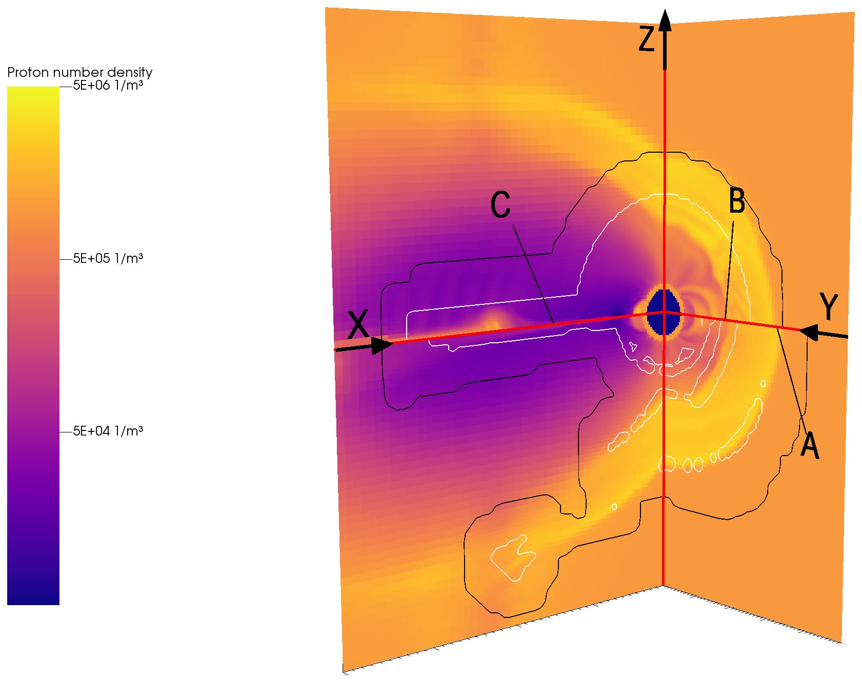
Figure 1 Overview of the global magnetospheric domain, tail side x–z and y–z planes in geocentric solar ecliptic (GSE) coordinates, with x positive sunwards and z northwards perpendicular to the ecliptic plane. A is the bow shock, B the magnetopause, and C the tail current sheet; these three regions are of particular interest, with variables changing rapidly over a short distance. The variable plotted is proton number density, with two levels of refinement contours on top: the inside of the region outlined in black has higher resolution than the outside, and the inside of the white outlines has the highest resolution. Two runs are plotted here, separated by the x–y plane marked by the horizontal red lines. The north side (above) is from a control run using static refinement, and the south side (below) is from a run using adaptive refinement. Physical differences can be seen in the subsolar shock, magnetopause, and tail; these are artefacts of the lower initial resolution of the AMR run.

2 Methods

2.1 Spatial refinement

The sparse velocity space described in Sect. 1.1 is sufficient for hybrid simulations in two spatial dimensions, but three-dimensional simulations require additional spatial optimizations. The method used is cell-based spatial refinement, implemented in Vlasiator 5 (Pfau-Kempf et al., 2024) in a static manner by parametrizing regions to simulate at a finer spatial resolution (Ganse et al., 2023). The adaptive grid is provided by a library called the distributed Cartesian cell-refinable grid (DCCRG; Honkonen, 2023), which also communicates data between processes and provides an interface for the load balancing library Zoltan (Devine et al., 2002). Each cell keeps track of the processes that cells in its neighbourhood belong to, allowing remote communication.

Initially, each cubic cell starts at refinement level 0. These cells are refined by splitting them into eight equally sized cubic children, i.e. splitting them in half along each Cartesian direction. The children of a cell have a refinement level that is one higher than their parent. DCCRG cells have a neighbourhood defined by a distance of the cell's own size for ghost data. Vlasiator's semi-Lagrangian solver has a stencil width of two cells, and a neighbourhood of three cells is used to catch all edge cases. Neighbours are required to be at most one refinement level apart, so a cell of level 0 has a minimum of six level 1 cells between itself and a level 2 cell (Honkonen et al., 2013). If this condition is not met, for example if a level 1 cell with level 0 neighbours is refined, DCCRG resolves this by inducing refinement in the refined cell's neighbours. In case refining a cell is not possible due to, for example, boundary limitations, refinement is cancelled. Effectively, the last refinement change takes precedence. The grid also has a maximum refinement level given as a parameter.

Static refinement is configured to refine a sphere around the inner boundary up to level 2 and the tail box and the nose cap up to level 3. This is done when starting a simulation run, and the refinement remains constant throughout. The spherical refinement and nose cap are meant to catch the magnetopause and the tail box the magnetotail current sheet. The top half of Fig. 1 shows this static refinement, with the two slices shown in full in Fig. 2. The performance gains of this method are demonstrated by Ganse et al. (2023).

Note that spatial refinement is only applied to the 3D spatial grid containing the distribution function. Updating the electromagnetic field is relatively cheap, so the field solver grid is homogeneous, matching the maximum refinement level of the Vlasov grid. After each Vlasov solver time step, moments of the distribution function are copied over to the field solver grid, to multiple field solver cells in case of resolution mismatch. These moments are used to evolve the field, and after the field solver time step, fields are copied from the field solver grid to the Vlasov grid, taking an average if necessary. To prevent sampling artefacts, a low-pass filter is used when the local resolutions do not match (Papadakis et al., 2022).

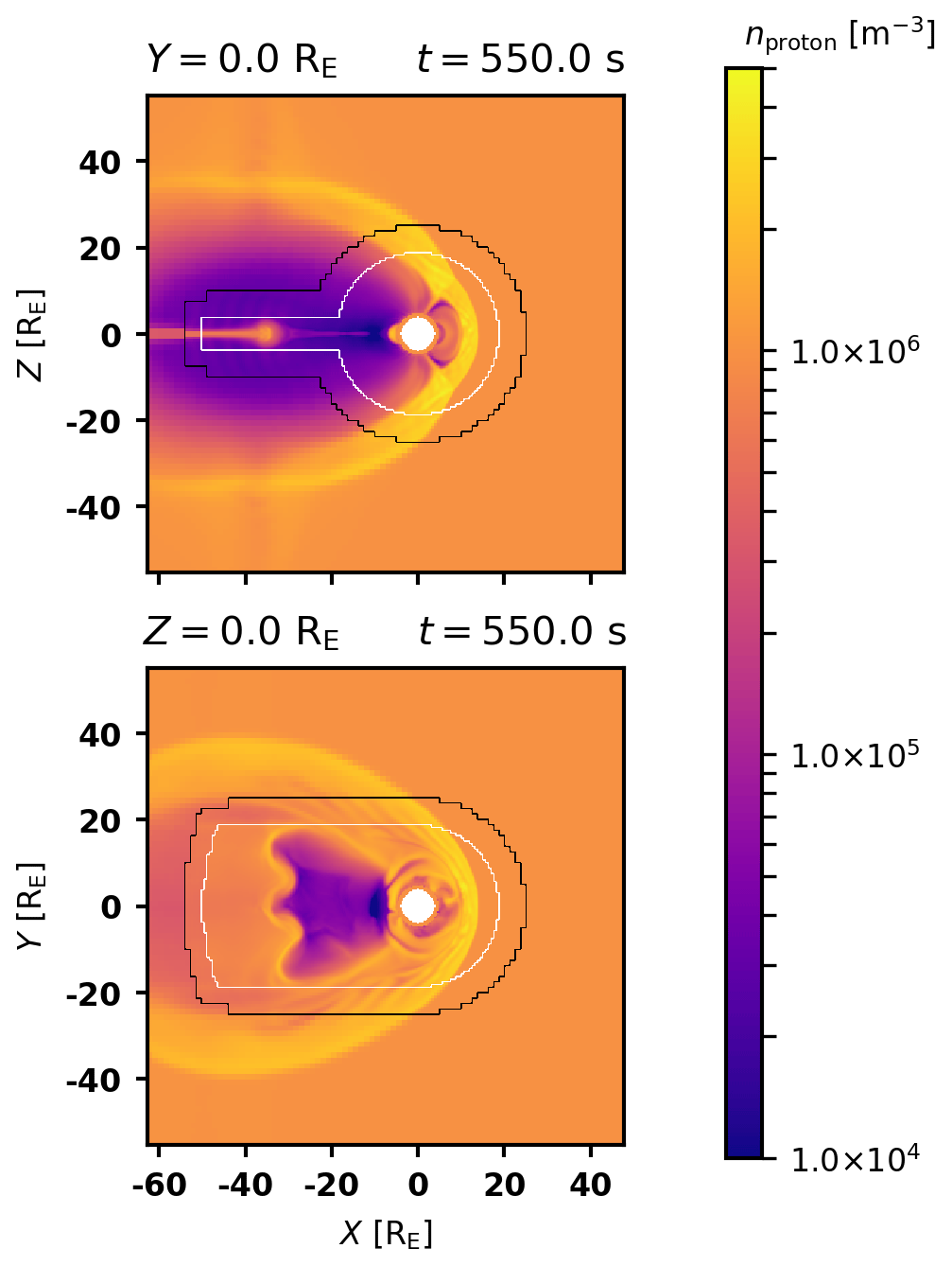
Figure 2 Contour plot of static refinement on particle density, with two slices. Note that the spherical refinement does not follow the shape of the shock; the second refinement level extends outside it and is circular rather than an arc.

2.2 Shortcomings of static refinement

Examining Fig. 2 reveals some issues with static refinement. Note that the parametrized spherical region does not follow the shape of the shock exactly; in this case, an elliptic shape would refine less of the spatially homogeneous solar wind and catch more shock dynamics.

We may also consider situations where the refinement parameters fit poorly. Solar wind is not static, so under varying conditions, the regions of interest may shift. Refinement regions are symmetric with respect to the x–y and x–z planes, so they do not perfectly fit structures for an oblique solar wind or tilted geomagnetic dipole field either. Reparametrization is not too difficult using trial and error, but it is unnecessary work for the end user. In a dynamic simulation, we might even find these regions shifting during a single run, making a static refinement from start to finish necessarily suboptimal. A solution to these issues is to use adaptive mesh refinement for dynamic runtime refinement. With properly chosen parameters, refinement should be better optimized, easier to tune, and more adaptive to changing conditions. Re-refining with sufficient frequency also allows following dynamic structures. Quantitative comparisons between the refinement methods are given in Sect. 3.

2.3 Refinement indices

We first introduce the refinement index α₁, a maximum of changes in spatial variables based on the index used in GUMICS (Janhunen et al., 2012):

$$\begin{array}{}\text{(1)}& {\mathit{\alpha }}_{\mathrm{1}}=\max \left\{\begin{array}{ll}\frac{\left|\mathrm{\Delta }\mathit{\rho }\right|}{\widehat{\mathit{\rho }}}& \left(\mathrm{a}\right)\\ \frac{\left|\mathrm{\Delta }U\right|}{\widehat{U}}& \left(\mathrm{b}\right)\\ \frac{(\mathrm{\Delta }\mathit{p}{)}^{\mathrm{2}}}{\mathrm{2}\mathit{\rho }\widehat{U}}& \left(\mathrm{c}\right)\\ \frac{(\mathrm{\Delta }\mathit{B}{)}^{\mathrm{2}}}{\mathrm{2}{\mathit{\mu }}_{\mathrm{0}}\widehat{U}}& \left(\mathrm{d}\right)\\ \frac{\left|\mathrm{\Delta }\mathit{B}\right|}{\widehat{B}}.& \left(\mathrm{e}\right)\end{array}\right.\end{array}$$

These variables are (a) particle density; (b) total, (c) plasma, and (d) magnetic field energy density scaled to total energy density; and (e) magnetic flux density. The contribution of the electric field energy density is considered negligible:

$$\begin{array}{}\text{(2)}& U\approx {\displaystyle \frac{{\mathit{p}}^{\mathrm{2}}}{\mathrm{2}\mathit{\rho }}}+{\displaystyle \frac{{\mathit{B}}^{\mathrm{2}}}{\mathrm{2}{\mathit{\mu }}_{\mathrm{0}}}}.\end{array}$$

In GUMICS, the magnetic field of the Earth's dipole is removed from B, leaving the perturbed field B₁ in the determination of these ratios. In Vlasiator we find that better refinement results from using the full magnetic field in Eq. (1). The simulation is given a refinement threshold and a coarsening threshold as parameters; for example a cell might be coarsened if α₁<0.3 and refined if α₁>0.6.

The way this works is each cell is compared pairwise to all cells that share a face with it, with Δa being the difference and $\widehat{a}$ the maximum in quantity a between those two cells. The maximum of all these comparisons is the final value of α₁.

Plots of the constituents of α₁ in the x–z plane near the x axis are given in Fig. 3. Comparing this to Fig. 2, the magnetotail and dayside magnetopause are clearly visible along with the front of the shock, but the inner magnetosphere is less highlighted.

A second refinement index is derived from current density and the magnetic field:

$$\begin{array}{}\text{(3)}& {\mathit{\alpha }}_{\mathrm{2}}={\displaystyle \frac{{\mathit{\mu }}_{\mathrm{0}}\left|\mathit{J}\right|}{B_{⟂}+\mathit{ϵ}}}\mathrm{\Delta }x,\end{array}$$

where $\mathit{J}=\frac{\mathrm{1}}{{\mathit{\mu }}_{\mathrm{0}}}\mathrm{\nabla }\times \mathit{B}$ is the current density in the cell, B_⟂ the density of the magnetic field perpendicular to the current, ϵ a small constant to avoid dividing by zero, and Δx the edge length of the cell. This is used to detect magnetic reconnection regions in the MHD-AEPIC model (Wang et al., 2022) in order to embed PIC regions, which is similar in aim to the spatial refinement sought in this work. Consider that α₂ is dimensionless: $B_{⟂}/\left|\mathit{J}\right|$ gives a characteristic length scale, which is compared to Δx. We can again use a refinement and coarsening threshold as with α₁.

As the framework for adaptive runtime refinement is implemented, developing new refinement indices is simple. So far, the Larmor radius r_L and the ion inertial length d_i have been evaluated but have been deemed to be less usable on their own than the current indices. Combining them to an aggregate index in a similar way to α₁ could prove useful and will be the topic of further investigations.

2.4 Interpretation of refinement thresholds

Refinement thresholds have a physical meaning as the maximum allowed gradient or perpendicular current in a cell before it is refined. A useful formulation would be to consider the target refinement level that a cell would be refined towards. The term α₂ has an explicit dependency on Δx, while the constituents of α₁ can generally be written as $\frac{\mathrm{\nabla }y}{\widehat{y}}\mathrm{\Delta }x$. Taking a general refinement parameter α:=yΔx, its refinement criterion for a threshold b is

$$\begin{array}{}\text{(4)}& \begin{array}{rl}\mathit{\alpha }:=y\mathrm{\Delta }x& >b\\ y\mathrm{\Delta }{x}_{\mathrm{0}}\cdot {\mathrm{2}}^{-r}& >b\\ y\mathrm{\Delta }{x}_{\mathrm{0}}& >b\cdot {\mathrm{2}}^r\\ {\log }_{\mathrm{2}}\left(y\mathrm{\Delta }{x}_{\mathrm{0}}\right)& >{\log }_{\mathrm{2}}b+r\\ {\mathit{\alpha }}^{\prime }:={\log }_{\mathrm{2}}\left(y\mathrm{\Delta }{x}_{\mathrm{0}}\right)-{\log }_{\mathrm{2}}b& >r,\end{array}\end{array}$$

with the substitution $\mathrm{\Delta }x=\mathrm{\Delta }{x}_{\mathrm{0}}\cdot {\mathrm{2}}^{-r}$ using the zeroth level cell size Δx₀ and refinement level r. Thus, we can define α^′ as the target refinement level of the cell.

With this rescaling, we now have a modified index where a cell's target refinement level is at least α^′, which can be calculated straightforwardly using the original index α and its refinement threshold b. This also gives the natural choice of the unrefinement threshold as $b/\mathrm{2}$. In practice, a cell would be refined if ${\mathit{\alpha }}^{\prime }>r$ and unrefined if ${\mathit{\alpha }}^{\prime }<r-\mathrm{1}$, with log ₂b as a shift parameter.

The logical meaning of negative values is that the ideal cell size in a region is larger than the coarsest level of refinement in the grid. In practice increasing the size of the coarsest cells is not necessary, as these regions typically have the fewest velocity space cells and contribute little to the overall computational load. A very large value of Δx₀ would also cause issues with induced refinement. In the configuration used in this work, a cell of level −7 would be larger than the entire grid, while having a single cell of level −5 would limit the maximum refinement found anywhere within the domain to −3.

Plots of ${\mathit{\alpha }}_{\mathrm{1}}^{\prime }$ and ${\mathit{\alpha }}_{\mathrm{2}}^{\prime }$ are given in Fig. 4. Comparing them to Fig. 2, the indices are more narrowly localized to the tail current sheet, shock, and magnetopause than the static refinement. Additionally, a flank foreshock at $x\approx -\mathrm{30}{R}_{\mathrm{E}}$ is picked up by both indices; refining such moving structures is impossible using static refinement. The two indices are somewhat similar but distinct; particularly the subsolar shock is resolved better by α₁, as α₂ focuses on detecting current sheets which do not occur on the shock surface.

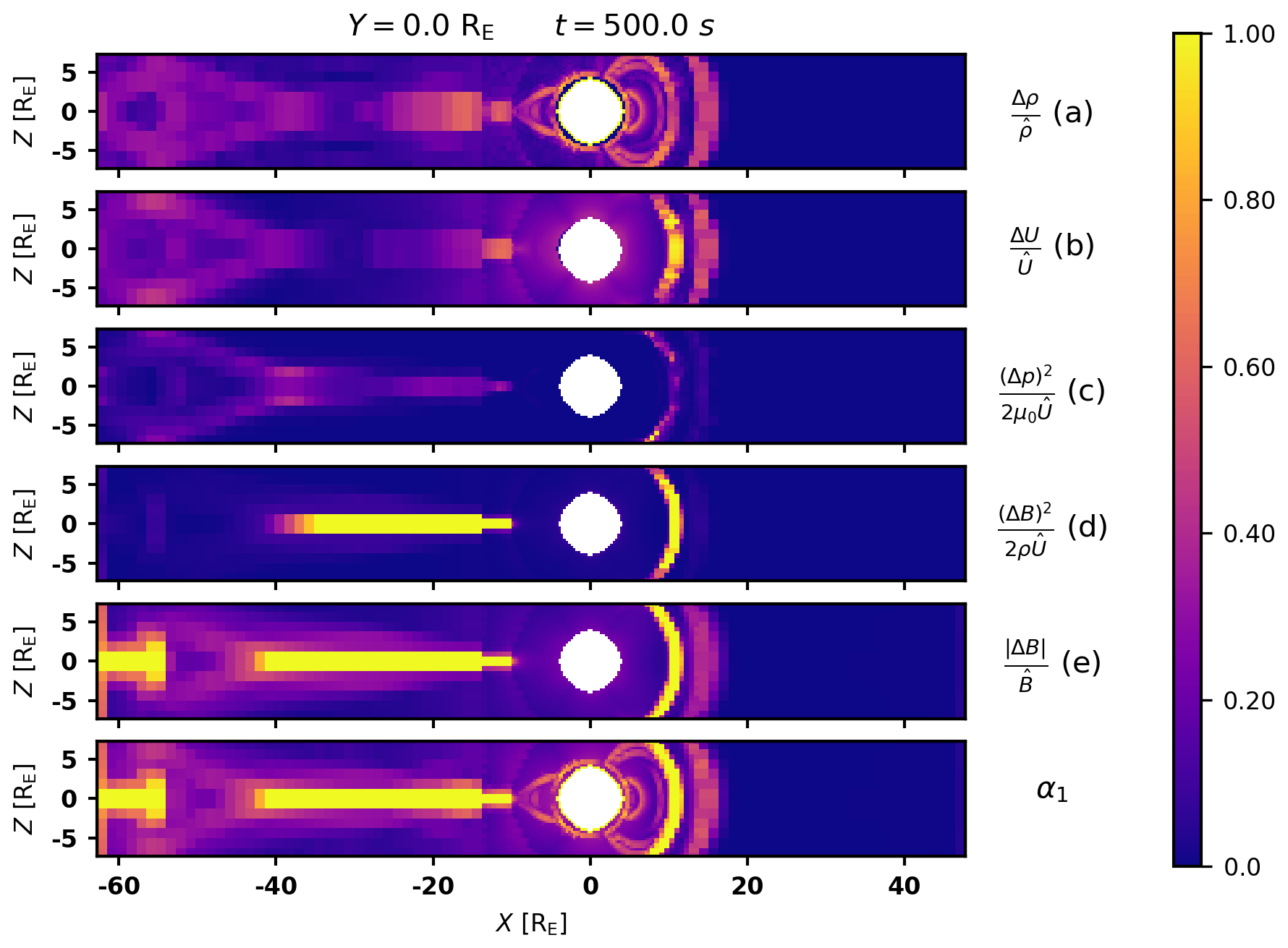
Figure 3 Plots of the constituent gradients of α₁ near the x axis at y=0, and their maximum α₁. Letters correspond to Eq. (1). Gradients are clipped to a maximum of 1, as this is the maximum of (a) and (b). Particle density (a) and total energy density (b) seem to discern the magnetopause and shock, while the field energy density (d) and magnetic flux density (e) highlight the magnetopause and tail current sheets. Kinetic energy density (c) seems to have a minor effect on the value of α, highlighting regions that are similar but with lower value compared to the other parameters.

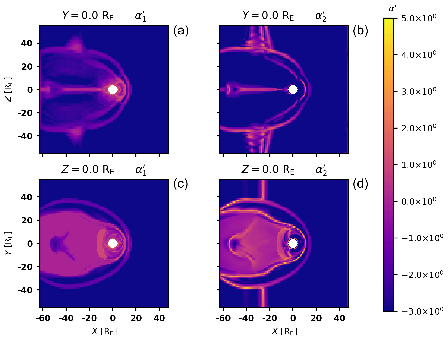
Figure 4 Plots of ${\mathit{\alpha }}_{\mathrm{1}}^{\prime }$ (a, c) and ${\mathit{\alpha }}_{\mathrm{2}}^{\prime }$ (b, d) on the x–z (a, b) and x–y (c, d) planes. Both indices highlight the magnetopause, particularly the subsolar region. Both indices also highlight the shock: α₁ highlights the subsolar shock better and α₂ the flanks and the flank foreshocks at $x\approx -\mathrm{30}{R}_{\mathrm{E}}$.

2.5 Implementation

The refinement procedure is as follows:

1. Each process calculates the refinement indices for all its cells.

2. Each process iterates over its cells, marking them for refinement or coarsening based on the indices.

3. The requirement of neighbouring cells having a maximum refinement level difference of 1 is imposed by DCCRG, inducing additional refinement.

4. The memory usage after refinement is estimated before execution. If this exceeds the memory threshold set for the simulation, the run tries to rebalance the load according to the targeted refinement. If it is still estimated that the run will exceed the memory threshold, the run exits so that the simulation may be restarted from that point with more resources or less aggressive refinement.

5. Refinement is executed. Refined cells are split into eight children with the distribution copied over, and coarsened cells are merged with the distribution averaged between eight siblings.

6. The moments are calculated for coarsened cells, and coordinate data are set for all new cells.

7. The computational load is balanced between the processes, and remote neighbour (ghost cell) information is updated.

Mesh refinement prefers refinement over coarsening. If either refinement index passes its refinement threshold, the cell is refined. A cell is coarsened only if both indices for the cell and all its siblings pass their coarsening threshold. This overrides DCCRG behaviour for induced refinement; a cell will not be unrefined if that would result in the unrefinement of any cell above its coarsening threshold. Alternatively, either refinement index may be disabled, in which case the other controls the refinement entirely. There is also additional bias against isolated, unrefined cells: a cell is always refined if a majority of its neighbours are refined, and cells are never unrefined in isolation; cells are only unrefined if they have either coarser neighbours or neighbours that would also be unrefined.

Mesh refinement may be limited to a specific distance from the origin to limit refinement to where it is most relevant for the simulation; refinement is still induced outside this, as refining a cell on the boundary to the second level requires cells outside to be on the first level and so on. Refinement may also be started at a specific time after the beginning of the simulation. This enables simulating initial conditions using a coarse grid and refining after a certain time without user intervention.

Boundary cells are not refined or unrefined dynamically, since this makes the refinement simpler and the code easier to maintain due to not having to factor in boundary conditions. Therefore it is recommended to initially refine the inner boundary region up to the desired level, similarly to static refinement.

Refinement may be done automatically during runtime or manually by creating a file named DOMR in the run directory. As refinement requires load balancing, it is done before load balancing at user-set intervals. Refinement cadence thus depends on the load balance interval.

3 Results

3.1 Refinement

Runtime adaptive refinement was tested using similar parameters to a two-level test run shown in Fig. 2. The physical parameters were as specified in Sect. 1.1 but with a maximum resolution of 2000 km, as the tests were performed with two levels of refinement as opposed to three used on production runs.

Using only α₁, three test runs were done using refinement thresholds of 0.6, 0.4, and 0.2 with the unrefinement threshold set to half the refinement threshold. These test runs are referred to as alpha1-low, alpha1-med, and alpha1-high respectively. Similarly, using only α₂, three test runs were done using the same refinement and unrefinement thresholds. These are referred to as alpha2-low, alpha2-med, and alpha2-high. The option of delaying refinement was utilized to initialize the simulation with minimal refinement, and refinement was enabled from 500 s onwards. Refinement was restricted to a radius of 50 R_E from the origin. The runs alpha1-med and alpha2-med have final phase-space cell counts closest to that of the control run (1.058×10¹¹), yielding good points of comparison.

A quantitative comparison of the runs is provided in Fig. 5. Panels (a) and (b) show the behaviour of the phase-space cell count on AMR runs. With minimal refinement, the cell count and computational load are consistently lower than on the control run. Notably the medium AMR runs with a cell count comparable to the control have more level 1 cells and fewer level 2 cells than the control run; isolated regions of level 2 cells cause comparatively more induced refinement. The stacked histograms in panels (c) and (d) showing spatial volume for each refinement level as a function of α₁ are a validation of α₁ refinement, while histograms in panels (e) and (f) likewise show the same for α₂ and validate α₂ refinement. The runs alpha1-med and alpha2-med have few level 2 cells below the unrefinement threshold of 0.2 compared to the control run, as well as having no cells below level 2 above the refinement threshold of 0.4. There are many level 1 cells below the unrefinement threshold, likely due to induced refinement. The number of cells above the refinement threshold is also reduced overall, as smaller cells end up with lower cell-to-cell differences in variables compared to larger cells. Stacked histograms in panels (g) through (j) show the same runs using the α^′ indices or target refinement levels (Eq. 4). As expected, there are sharp limits at ${\mathit{\alpha }}^{\prime }=\mathrm{0}$, above which there are no cells below level 1, and ${\mathit{\alpha }}^{\prime }=\mathrm{1}$, above which there are no cells below level 2.

Examining plots of alpha1-med and alpha2-med in the x–y and x–z planes (Fig. 6), adaptive refinement follows the structures of the magnetosphere better than static refinement. The spherical region around the inner boundary seen in Fig. 2 is absent in both AMR runs, with refinement regions instead following the dayside magnetopause and shock. The tails of refinement also flare more widely in the x–y plane in both runs. In the case of α₁, refinement has left some disjoint regions inside the initial spherical refinement region. A smaller region of initial refinement might have avoided this issue. The results of the two refinement methods are somewhat similar but still distinct enough to warrant the usage of both. There are also notable physical differences between the control and AMR runs, particularly in the magnetotail. The reconnection rate is likely affected by numerical resistivity caused by the lower resolution during the 500 s initialization phase. Running the simulation for longer with AMR enabled is likely to reduce these differences, but ultimately convergence can only be compared to a simulation resolving the entire grid at the highest resolution, which is not computationally feasible.

In terms of proton density, two flank foreshocks in the y–z plane can be seen, and adaptive refinement follows the moving structure. Comparing particle density to Fig. 2 reveals the structure is somewhat different, particularly in the x–y plane; coarse initialization changes the physical behaviour of the system, with the benefit of smaller resource usage.

Refinement was performed at every load balance, i.e. every 50 time steps. This corresponds to about half a second in simulation time. Since cell size is between 2000 and 8000 km in this simulation and solar wind plasma velocity is some hundreds of kilometres per second, refinement should occur faster than the movement of any structure. The cadence seems sufficient: refinement follows the flank foreshocks, and the general structure of refinement regions sets in quickly. Further testing is required to determine suitability in more dynamic conditions. These findings seem to suggest that this would only need an adjustment of cadence.

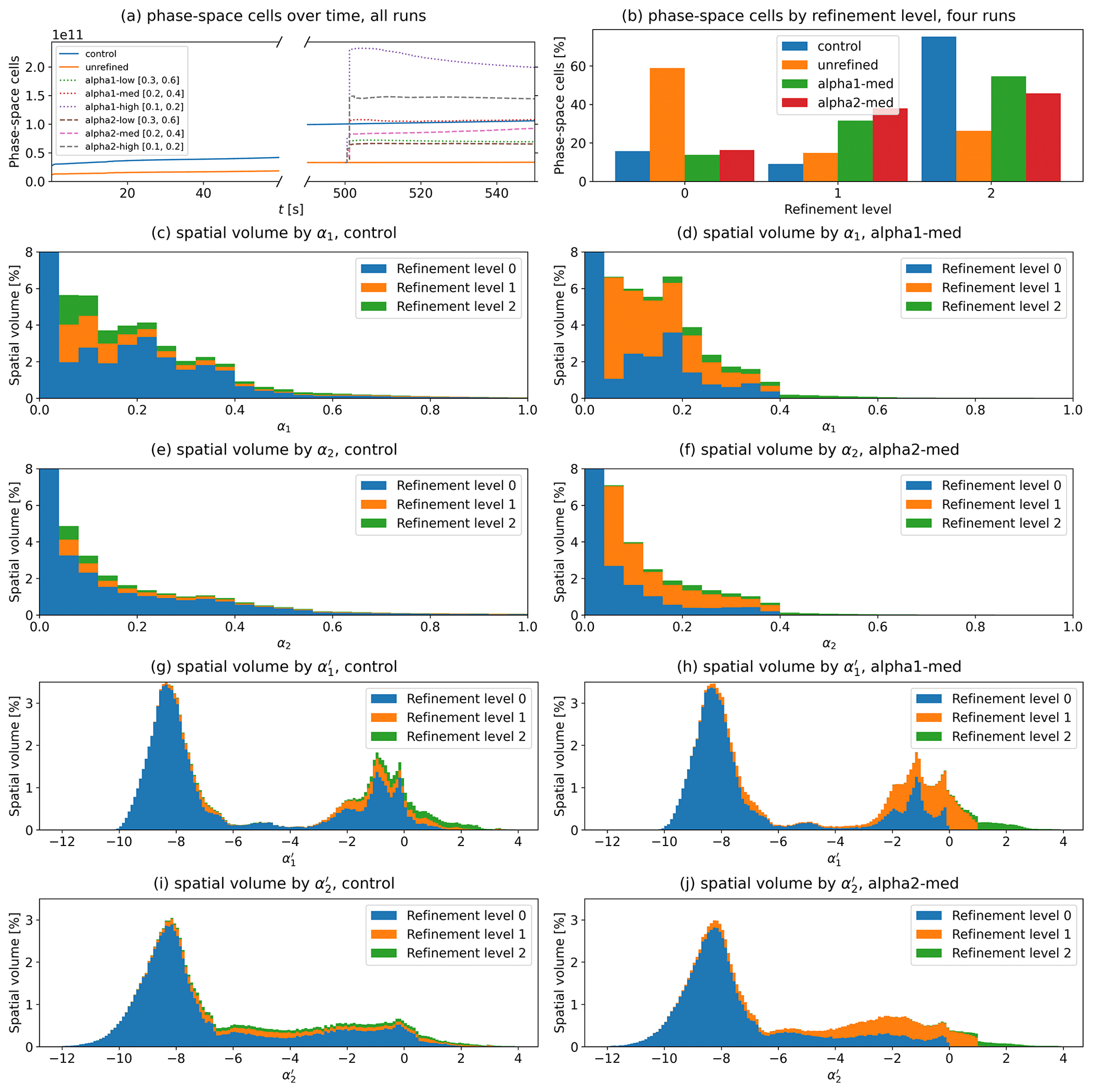
Figure 5 Ten plots of refinement-related parameters. Panel (a) shows the phase-space cell count over simulation time for the static runs and the six AMR runs with the unrefinement and refinement threshold in square brackets for the refined runs. Note that this includes velocity space, indicating the total computational load. Panel (b) shows the percentage of phase-space cells in each refinement level at the end of the static runs and both medium AMR runs (t=550 s). Panels (c)–(f) show stacked histograms of spatial volume by α₁ and α₂ in the control and medium AMR runs with the lowest bin of α<0.04 clipped. Panels (g)–(j) show stacked histograms of spatial volume by targeted refinement levels ${\mathit{\alpha }}_{\mathrm{1}}^{\prime }$ and ${\mathit{\alpha }}_{\mathrm{2}}^{\prime }$ in the control and medium AMR runs.

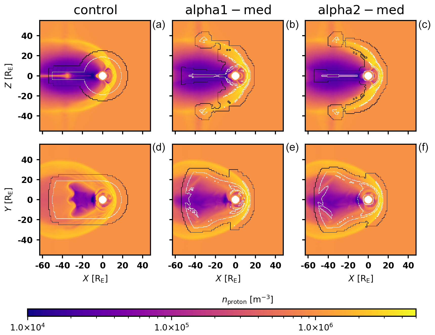
Figure 6 Contour plots of the refinement level on top of the particle density in the control (a, d), alpha1-med (b, e), and alpha2-med (c, f) runs (t=550 s; top panels, x–z plane; bottom panels, x–y plane). The run alpha1-med retains a large amount of the inner magnetosphere refined and has a clean level 2 boundary right on the bow shock. Meanwhile alpha2-med has less refinement in the inner magnetosphere but has more on the sides of the shock. A faint shape can be seen in proton density around $x=-\mathrm{20}$ to −40 R_E in the top panels; this is a flank foreshock that the refinement picks up, which has partially exited the refinement radius.

3.2 Performance

The runs were performed on the CSC Mahti supercomputer, utilizing CPU nodes with 256 GB memory and two AMD Rome 7H12 CPUs with 64 cores each for a total of 128 physical cores and 256 logical cores with hyperthreading. The unrefined run was on 32 nodes, while all the other runs were on 100 nodes due to their greater computational requirements. Each node ran 64 tasks for a total of four OpenMP threads per task. The task balance was kept constant as this was not the principal factor investigated.

Every run's performance was evaluated using the rate of cells solved per second per core. These data are provided in Table 1. The AMR runs have generally worse performance relative to the control run, with the comparative cell rate ranging from 62.6 % for alpha2-low to 99.9 % for alpha1-high. This implies that the increased grid complexity comes at a higher computational cost. There are two possible explanations for performance improving with cell count. First, as the problem size compared to core count increases, each process ends up spending more time in solving cells compared to communicating data with its neighbours, resulting in more ideal parallelization. Second, more refinement leads to more unified regions with fewer interfaces between unrefined and refined cells. This might be improved by using some heuristic to merge isolated regions of refinement, but it remains to be seen whether any simplification of the grid would offset the cost of additional phase-space cells.

Table 2 compares time spent in spatial translation and MPI wait times in runs alpha1-med and alpha2-med and the control; most of the time loss in translation is in waiting for other processes to finish translation in each direction. The load balancing method used was Zoltan's recursive coordinate bisection (Devine et al., 2002), with the velocity space cell count as the weight. This seems to work poorly for a complex grid due to either orthogonal cuts being non-ideal or the single weights not accounting for different translation times in each direction. Another possibility is poor weight calculation: weights are calculated on the step before load balancing, and the load balance after refinement uses the weight calculated for the parent, not accounting for changing refinement interfaces. Since refinement was performed at every load balance in these tests, every load balance was suboptimal, at least until the grid had settled to a point where few cells were refined on each pass. Load balancing between refinement passes is expected to alleviate this issue, and reducing the cadence of refinement without compromising the capture of spatial evolution is a matter of parameter optimization. It remains to be seen if this problem persists on a production-scale run with more tasks.

Of particular note is the performance of the initial 500 s of simulation, done with minimal refinement with only the inner boundary region refined to level 2. The total phase-space cell count reached at 500 s was 3.298×10¹⁰, with roughly the same number of cells solved per core second as the control run on 4096 cores. Initializing the simulation with minimal static refinement is thus quite efficient, using only a third of the resources of static refinement shown in Fig. 2. This performance benefit is expected to increase when refining a simulation up to level 3 or more.

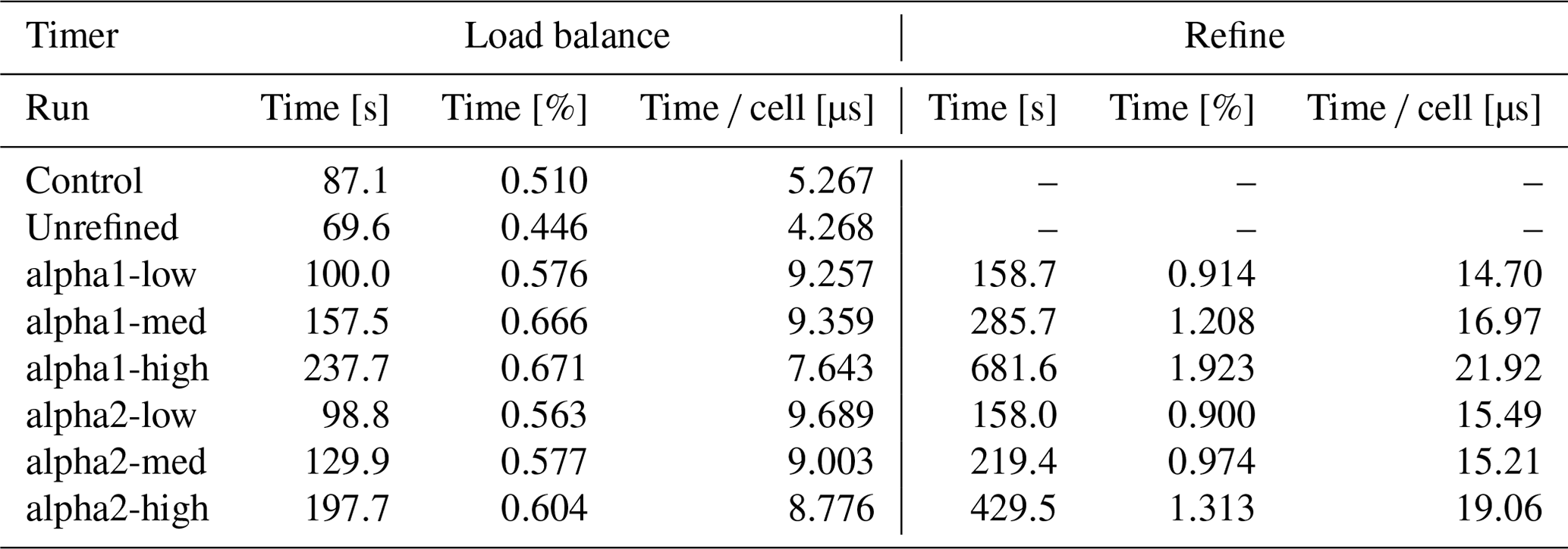
Table 3 shows the time taken in load balance and refining in each run. Balancing the load every 50 time steps and refining before each load balance, re-refining took on average 1.2 % of the simulation time in the run alpha1-med. In comparison, load balancing took 0.67 %, so refining almost triples the overhead compared to just rebalancing. However, load balancing itself took 81 % more time on the alpha1-med run, indicating that the refined grid is harder to partition. Splitting a cell effectively increases its load balance weight 8-fold; if a task domain contains a large number of refined cells, this increases the amount of communication required to balance the load. This effect is not limited to tasks where cells are refined: as these tasks migrate cells to neighbouring tasks, they will also have to migrate cells to other tasks in order to balance the load. Scaled to the phase-space cell count, the effect on load balancing is smaller in the alpha1-high run, indicating similar reasons to those for the overhead in translation performance. On the other hand, refinement time per cell grows with grid size; this is likely due to additional checks for induced refinement in DCCRG. As the total spatial cell count in the grid grows with refinement, each process has more cells, and each refined cell has more neighbours to check for induced refinement.

Table 1 Table of rates of phase-space cells solved per second and per core in each run over 500 to 550 s. The cell rate is generally worse for AMR runs but improves for runs with more refinement. The total runtime is given for reference, with the alpha1-med and alpha2-med runs closest to the computational load of control.

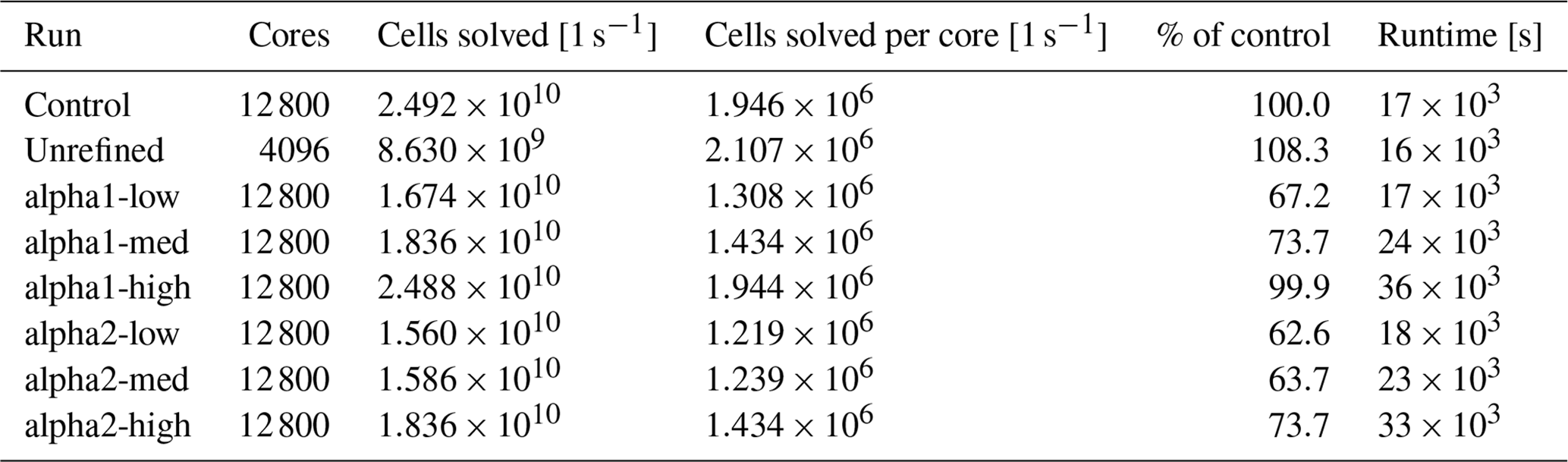
Table 2 Comparison of the time spent in spatial translation and specific timers within the alpha1-med and control runs. Vlasiator performs translation one dimension at a time, updating ghost cells in between. Pre-update barriers refer to the time spent by processes waiting for other processes to complete translation in order to update ghost cells. These waiting times account for 77 % of the time difference between alpha1-med and the control and 90 % between alpha2-med and the control.

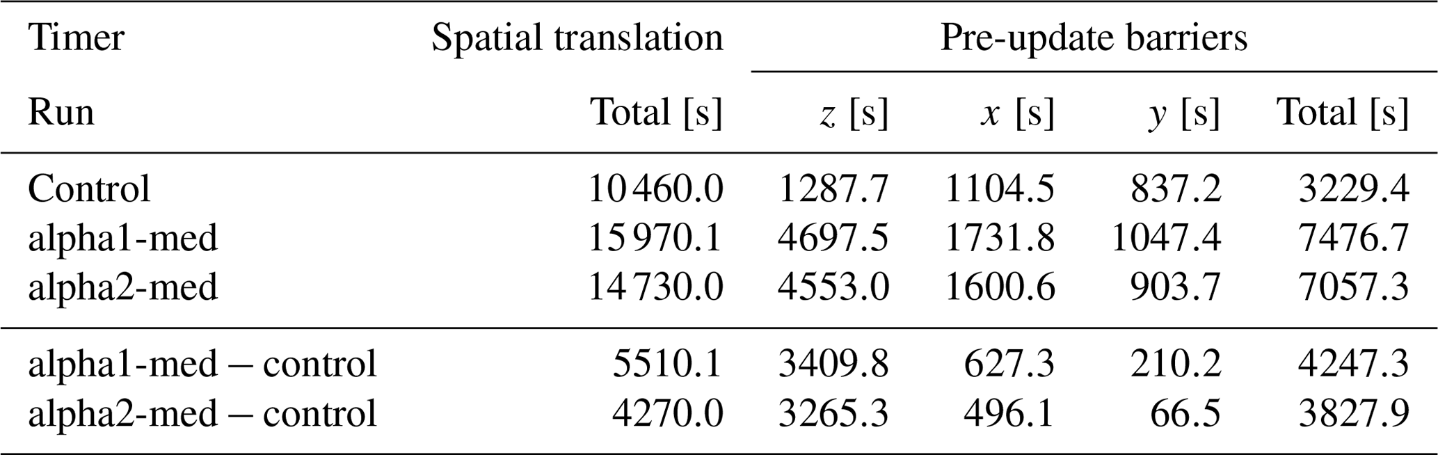
Table 3 Table of the time taken in load balance and refinement in seconds and the percentage of simulation time and microseconds per phase-space cell over 500 to 550 s. Load is balanced every 50 time steps in each run, with the AMR runs refined before every load balance. Load balancing takes somewhat longer on AMR runs, with the worst results on the runs with cell counts closest to the control.

4 Conclusions

In this paper we introduced a method to automatically adapt the Vlasiator spatial grid to concentrate numerical accuracy in regions of special interest. The method is based on two indices α₁ and α₂, measuring the rate of change in spatial variables and the occurrence of current sheets respectively. The grid is refined to a higher resolution in regions where these indices are high and coarsened to a lower resolution where they are low.

We also tested the performance of adaptive mesh refinement, and the results in Sect. 3 show this method works well for global simulations with some caveats. The option to delay refinement alone cuts computational load of the initialization phase to one-third in the test setup, as demonstrated in Table 1, and AMR produces good refinement, albeit with a notable performance overhead of around 26 % in the test case most similar to the control. Since the performance difference between the control and AMR runs seems to be primarily caused by load imbalance, developing better load balance criteria and methods might help alleviate the issue.

Another possibility is to consider different refinement parameters. Replacing them in the simulation code is simple now that the groundwork for AMR has been laid. As the current criteria borrow heavily from (1) GUMICS and MHD-AEPIC and (2) magnetohydrodynamic and embedded PIC simulations respectively, they might not be optimal for a Vlasov simulation. As both refinement indices are based on spatial variables, they do not explicitly account for kinetics present in the simulation. Implementing kinetic measures such as non-Maxwellianity (Graham et al., 2021) or agyrotropy (Swisdak, 2016) would efficiently indicate regions where kinetic phenomena dominate but would not directly map to dimensionless gradients. Thus, refining those regions would not bring the evaluated parameter into the requested range, and implementing them as refinement criteria is not straightforward.

Adaptive mesh refinement fulfils the goals set in its development: replacing static refinement with an adaptive and efficient algorithm. We plan to use AMR in upcoming large-scale production runs, providing further information on the method's advantages and shortcomings. In particular, initializing a simulation at a low resolution allows for a longer total simulated time using the same quantity of resources; however, care must be taken so that this does not compromise the simulation results.

Appendix A: Reproducing the data

The data may be reproduced in the following manner using the provided configuration (Kotipalo, 2023):

1. Install and compile Vlasiator using the instructions provided at https://github.com/fmihpc/vlasiator/wiki/Installing-Vlasiator (last access: 23 August 2024).

2. To generate the control data, run Vlasiator in the control directory using the corresponding configuration files via, for example, srun BIN -run_config control.cfg, where BIN is the Vlasiator executable.

3. To generate the unrefined data, run Vlasiator in the unrefined directory first using the configuration file unrefined-500s. Run it again using the configuration file unrefined-550s using the restart file created at 500 simulation seconds via, for example, srun BIN --run_config unrefined_550s.cfg --restart.filename restart/FILENAME, where FILENAME is the restart file.

4. To generate each AMR data point, run Vlasiator in each of the alpha1 and alpha2 directories using the corresponding configuration files and the same restart file as used for unrefined-550s.

5. The data in Tables 1, 2, and 3 are given by the script data.sh. Data for each run are given by ./data.sh RUN, where RUN is the path of the run to analyse.

6. The first three lines of output correspond to the first three columns of Table 1. The last column is the ratio of cells solved per core to the corresponding number of the control run.

7. The first four columns of Table 2 correspond to the timers Spatial-space and barrier-trans-pre-update_remote{z,x,y}. The average value in seconds is used here, with the total for pre-update barriers calculated as the sum of the z, x, and y barriers, and the difference is simply the difference between the two runs.

8. The columns “Load balance” and “Refine” in Table 3 correspond to the timers Balancing load and Re-refine spatial cell. The values used are average time, percentage of time, and time per phase-space cell.