the Creative Commons Attribution 4.0 License.
the Creative Commons Attribution 4.0 License.
 | 30 Aug 2024
Assimilation of carbonyl sulfide (COS) fluxes within the adjoint-based data assimilation system – Nanjing University Carbon Assimilation System (NUCAS v1.0)
Huajie Zhu
Mousong Wu
Fei Jiang
Michael Vossbeck
Thomas Kaminski
Xiuli Xing
Weimin Ju
Jing M. Chen
Modeling and predicting changes in the function and structure of the terrestrial biosphere and its feedbacks to climate change strongly depends on our ability to accurately represent interactions of the carbon and water cycles and energy exchange. However, carbon fluxes, hydrological status, and energy exchange simulated by process-based terrestrial ecosystem models are subject to significant uncertainties, largely due to the poorly calibrated parameters. In this work, an adjoint-based data assimilation system (Nanjing University Carbon Assimilation System; NUCAS v1.0) was developed, which is capable of assimilating multiple observations to optimize process parameters of a satellite-data-driven ecosystem model – the Biosphere–atmosphere Exchange Process Simulator (BEPS). Data assimilation experiments were conducted to investigate the robustness of NUCAS and to test the feasibility and applicability of assimilating carbonyl sulfide (COS) fluxes from seven sites to enhance our understanding of stomatal conductance and photosynthesis. Results showed that NUCAS is able to achieve a consistent fit to COS observations across various ecosystems, including evergreen needleleaf forest, deciduous broadleaf forest, C3 grass, and C3 crop. Comparing model simulations with validation datasets, we found that assimilating COS fluxes notably improves the model performance in gross primary productivity and evapotranspiration, with average root-mean-square error (RMSE) reductions of 23.54 % and 16.96 %, respectively. We also showed that NUCAS is capable of constraining parameters through assimilating observations from two sites simultaneously and achieving a good consistency with single-site assimilation. Our results demonstrate that COS can provide constraints on parameters relevant to water, energy, and carbon processes with the data assimilation system and opens new perspectives for better understanding of the ecosystem carbon, water, and energy exchanges.
- Article
(5291 KB) - Full-text XML
-
Supplement
(3867 KB) - BibTeX
- EndNote


Overwhelmingly due to anthropogenic fossil fuel and carbonate emissions, as well as land use and land cover change (Arias et al., 2021), atmospheric carbon dioxide (CO2) concentrations have increased at an unprecedented rate since the Industrial Revolution, and the global climate has been profoundly affected. As a key component of the Earth system, the terrestrial biosphere has absorbed about 30 % of anthropogenic CO2 emissions since 1850 (Friedlingstein et al., 2022). However, in line with large-scale global warming, the structure and function of the terrestrial biosphere have changed rapidly (Grimm et al., 2013; Arias et al., 2021; Moore and Schindler, 2022). As a consequence, terrestrial carbon fluxes are subject to great uncertainty (MacBean et al., 2022).
Terrestrial ecosystem models have been an important tool used to investigate the net effect of complex feedback loops between the global carbon cycle and climate change (Zaehle et al., 2005; Fisher et al., 2014; Fisher and Koven, 2020). Meanwhile, with the advancement of modern observational techniques, a rapidly increasing number of satellite- and ground-based observational datasets have played an important role in studying the spatiotemporal distribution and mechanisms of the terrestrial ecosystem carbon fluxes (Rodell et al., 2004; Quirita et al., 2016). Observations, such as sun-induced chlorophyll fluorescence (Schimel et al., 2015) and soil moisture (Wu et al., 2018), have been used to estimate or constrain carbon fluxes in terrestrial ecosystems (Scholze et al., 2017). Carbonyl sulfide (COS) has emerged as a promising proxy for understanding terrestrial carbon uptake and plant physiology (Montzka et al., 2007; Campbell et al., 2008), since it is taken up by plants through the same pathway of stomatal diffusion as CO2 (Goldan et al., 1988; Sandoval-Soto et al., 2005; Seibt et al., 2010) and completely removed by hydrolysis without any back-flux in leaves under normal conditions (Protoschill-Krebs et al., 1996; Stimler et al., 2010).
Plants open/close leaf stomata in order to regulate the water and CO2 transit during transpiration and photosynthesis (Daly et al., 2004). As an important probe for characterizing stomatal conductance, COS has shown great potential to constrain plant photosynthesis and transpiration and to improve understanding of the water–carbon coupling (Wohlfahrt et al., 2012; Asaf et al., 2013; Wehr et al., 2017; Kooijmans et al., 2019; Sun et al., 2022; Zhu et al., 2024). A number of empirical or mechanistic COS plant uptake models (Campbell et al., 2008; Wohlfahrt et al., 2012; Berry et al., 2013) and soil exchange models (Kesselmeier et al., 1999; Berry et al., 2013; Launois et al., 2015; Sun et al., 2015; Whelan et al., 2016; Ogée et al., 2016; Whelan et al., 2022) have been developed to simulate COS fluxes in order to more accurately estimate gross primary productivity (GPP), stomatal conductance, transpiration. However, due to the lack of ecosystem-scale measurements of the COS flux (Brühl et al., 2012; Wohlfahrt et al., 2012; Kooijmans et al., 2021), only a few studies were conducted to systematically assess the ability of COS to simultaneously constrain photosynthesis, transpiration, and other related processes in ecosystem models.
Data assimilation is an approach that aims at producing physically consistent estimates of the dynamical behavior of a model by combining information in process-based models and observational data (Liu and Gupta, 2007; Law et al., 2015). It has been widely applied in geophysics and numerical weather prediction (Tarantola, 2005). In the past few decades, substantial efforts have been put into the use of satellite- (Knorr et al., 2010; Kaminski et al., 2012; Deng et al., 2014; Scholze et al., 2016; Norton et al., 2018; Wu et al., 2018) and ground-based (Knorr and Heimann, 1995; Rayner et al., 2005; Santaren et al., 2007; Kato et al., 2013; Zobitz et al., 2014) observational datasets to constrain or optimize the photosynthesis-, transpiration-, and energy-related parameters and variables of terrestrial ecosystem models via data assimilation techniques. More specifically, by applying data assimilation methods to process-based models, not only can the observed dynamics of ecosystems be more accurately portrayed, but our understanding of ecosystem processes can also be deepened with respect to their responses to climate changes (Luo et al., 2011; Keenan et al., 2012; Niu et al., 2014).
In this study, we present the newly developed adjoint-based Nanjing University Carbon Assimilation System (NUCAS v1.0). NUCAS v1.0 is designed to assimilate multiple observational data streams, including COS fluxes, to improve the process-based Biosphere–atmosphere Exchange Process Simulator (BEPS) (Liu et al., 1997), which has been specifically extended for simulating the ecosystem COS flux with the advanced two-leaf model that is driven by satellite observations of leaf area index (LAI).
In this context, the main questions that we aim to answer in this paper are as follows:
-
What parameters is the COS simulation sensitive to, and how do these parameters change in the assimilation of observed ecosystem-scale COS fluxes?
-
How effective is the assimilation of COS fluxes in improving the carbon, water, and energy balance for different ecosystems (including evergreen needleleaf forest, deciduous broadleaf forest, C3 grass, and C3 crop)?
-
Which processes are constrained by the assimilation of COS fluxes, and what are the mechanisms leading to adjustments of the corresponding process parameters?
-
How robust is NUCAS when optimizing over a single site and over two sites simultaneously?
To achieve these objectives, COS flux observations across a wide range of ecosystems (including evergreen needleleaf forest, deciduous broadleaf forest, C3 grass, and C3 crop) are assimilated into NUCAS to optimize the model parameters using the four-dimensional variational (4D-Var) data assimilation approach, and the optimization results are evaluated against in situ observations. Materials and methods used in our study are described in Sect. 2, which introduces the BEPS model and NUCAS, along with the data used to drive BEPS or for assimilation into NUCAS, and the parameters chosen to be optimized in this study. The results are presented in Sect. 3, including the fit of COS simulations to observations, the variation and impact of parameters on simulated COS, and the comparison and evaluation of model outputs. Section 4 discusses the impacts of the COS assimilation on parameters and processes related to the water–carbon cycle and energy exchange and discusses the influence of uncertain inputs, in particular, impacts of LAI on posterior parameter values. In addition, caveats and implications of assimilating COS flux are summarized. Finally, conclusions are laid out in Sect. 5.
2.1 NUCAS data assimilation system
2.1.1 NUCAS framework
NUCAS is built around the generic satellite-data-driven ecosystem model BEPS and applies the 4D-Var data assimilation method (Talagrand and Courtier, 1987). The BEPS model uses satellite-derived one-sided LAI to drive the phenology dynamics and separates sunlit and shaded leaves in calculating canopy-level energy fluxes and photosynthesis. It further features detailed representations of water and energy processes (Fig. 1). These features render BEPS more advanced in representing ecosystem processes than standard ecosystem models (Richardson et al., 2012) with fewer parameters to be calibrated owing to the LAI-driven phenology.
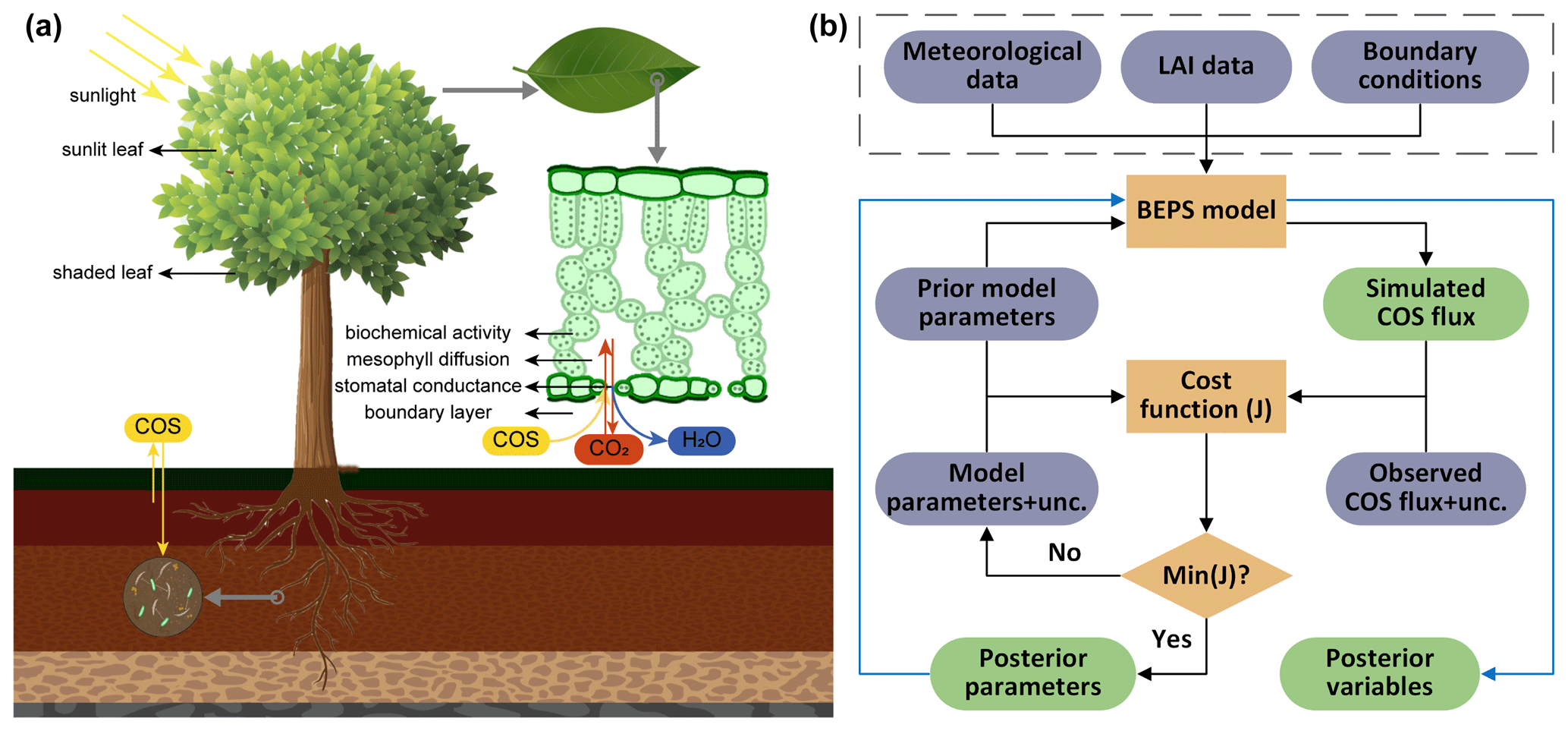
Figure 1Schematic of the Nanjing University Carbon Assimilation System (NUCAS). (a) Illustration of a two-leaf model coupling stomatal conductance, photosynthesis, transpiration, and COS uptake and an empirical model for simulating soil COS fluxes in NUCAS. (b) Data assimilation flowchart of NUCAS. Ovals represent input (blue-gray) and output (green) data. The boxes and rhombi represent the calculation and judgment steps. The solid black line represents the diagnostic process, the solid blue line represents the prognostic process, and the input datasets of BEPS (in the dashed box) are used in both the diagnostic process and the prognostic process.
Data assimilation is performed in two sequential steps: firstly, an inversion step adjusts the values of parameters controlling photosynthesis, energy balance, hydrology, and soil biogeochemical processes to match the observations. Secondly, the posterior parameters obtained in the first step are used as input data for the second step, in which the BEPS model is re-run to obtain the posterior model variables. The schematic of the system is shown in Fig. 1.
Considering model and data uncertainties, NUCAS implements a probabilistic inversion concept (Talagrand and Courtier, 1987; Tarantola, 1987, 2005) by using Gaussian probability density functions to combine the dynamic model and observations to obtain an estimate of the true state of the system and model parameters (Talagrand, 1997; Dowd, 2007). Hereby, we minimize the following cost function:
where O and M denote vectors of observations and their modeled counterparts, respectively, and x and x0 denote the control parameter vector with current and prior values, respectively. CO and Cx denote the uncertainty covariance matrices for observations and prior parameters. Both matrices are diagonal, expressing the assumption that observation uncertainties and parameter uncertainties are independent (Rayner et al., 2005). This definition of the cost function contains both the mismatch between modeled and observed COS fluxes and the mismatch between current and prior parameter values (Rayner et al., 2005).
To determine an optimal set of parameters which minimizes J, a gradient-based optimization algorithm performs an iterative search (Wu et al., 2020). In each iteration, the gradient of J is calculated by applying the adjoint of the model, where the model is run backward to efficiently compute the sensitivity of J and with respect to x (Rayner et al., 2005). The gradient of J is used to define a new search direction. The adjoint model is an efficient sensitivity analysis tool for calculating the parametric sensitivities of complex numerical model systems (An et al., 2016). The computational cost of it is independent of the number of parameters and is in the current case comparable to three to four evaluations of J. In this study, all derivative code is generated from the model code by the automatic differentiation tool TAPENADE (Hascoët and Pascual, 2013). The derivative with respect to each parameter was validated against finite differences of model simulations, which showed agreement within the accuracy of the finite difference approximation. The minimization of the cost function is implemented in a normalized parameter space where the parameter values are measured in multiples of their respective standard deviations with Gaussian priors (Kaminski et al., 2012). The model parameters are the various constants that are not influenced by the model state. Therefore, while they may change between plant function types (PFTs) to reflect different conditions and physiological mechanisms, they will not change in time (Rayner et al., 2005).
2.1.2 BEPS basic model
The BEPS model (Liu et al., 1997; Chen et al., 1999, 2012) is a process-based diagnostic model driven by remotely sensed vegetation data, including LAI, clumping index, and land cover type, as well as meteorological and soil data (Chen et al., 2019). With the consideration of coupling among terrestrial carbon, water, and nitrogen cycles (He et al., 2021), the BEPS model now consists of photosynthesis, energy balance, hydrological, and soil biogeochemical modules (Ju et al., 2006; Liu et al., 2015). It stratifies whole canopies into sunlit and shaded leaves to calculate carbon uptake and transpiration for these two groups of leaves separately (Liu et al., 2015). For each group of leaves, the GPP is calculated by scaling Farquhar's leaf biochemical model (Farquhar et al., 1980) up to canopy level with an updated temporal and spatial scaling scheme (Chen et al., 1999), and the stomatal conductance is calculated using a modified version of the Ball–Berry (BB) model (Ball et al., 1987; Ju et al., 2006). Evapotranspiration (ET) is calculated as the summation of sunlit leaf and shaded leaf transpiration, evaporation from soil and wet canopy, and sublimation from snow storage on the ground surface (Liu et al., 2003). The BEPS model stratifies the soil profile into multiple layers (five were used in this study) and simulates temperature and water content from each layer (Ju et al., 2006). The soil water content is then used to adjust stomatal conductance considering the water stress impacts (Ju et al., 2010; He et al., 2021). Over the last few decades, the BEPS model has been continuously improved and used for a wide variety of terrestrial ecosystems (Schwalm et al., 2010; Liu et al., 2015).
The previous version of BEPS considers a total of 6 PFTs and 11 soil textures (Chen et al., 2012). We use the same soil texture but added 4 PFTs to BEPS in order to better discriminate vegetation types, especially the C4 grass and C4 crop. Detailed information on these 10 PFTs and 11 soil textures is given in Table S1.
2.1.3 COS modeling
The ecosystem COS flux, FCOS,ecosystem, includes both plant COS uptake FCOS,plant and soil COS flux exchange FCOS,soil (Whelan et al., 2016). In this study, these two components were modeled separately. The canopy-level COS plant uptake FCOS,plant (pmol m−2 s−1) was calculated by upscaling the resistance analog model of COS uptake, as presented by Berry et al. (2013) with the upscaling scheme recommended by Chen et al. (1999). Specifically, considering the different responses of foliage to diffuse and direct solar radiation (Gu et al., 2002), FCOS,plant is calculated as
where LAIsunlit and LAIshaded are the LAI values (m2 m−2) of sunlit and shaded leaves, respectively. FCOS,sunlit and FCOS,shaded are the leaf-level COS uptake rate (pmol m−2 s−1) of sunlit and shaded leaves, respectively. The leaf-level COS uptake rate FCOS,leaf is calculated as
where COSa is the COS mole fraction in the bulk air and gsw and gbw are the stomatal conductance and leaf laminar boundary layer conductance to water vapor (H2O), respectively (Berry et al., 2013). The factors 1.94 and 1.56 account for the smaller diffusivity of COS with respect to H2O (Seibt et al., 2010; Stimler et al., 2010). The apparent conductance for COS uptake from the intercellular airspaces is denoted by gCOS and combines the mesophyll conductance and the biochemical reaction rate of COS and carbonic anhydrase (CA). Independent studies indicate that both CA activity and mesophyll conductance tend to scale with the photosynthetic capacity or the maximum carboxylation rate of Rubisco (Badger and Price, 1994; Evans et al., 1994), such that
where α is a parameter that is calibrated to observations of simultaneous measurements of COS and CO2 uptake (Stimler et al., 2012). Analysis of these measurements yields estimates of α of ∼1400 for C3 and ∼7500 for C4 species (Stimler et al., 2012; Haynes et al., 2020). According to the COS modeling scheme of the Simple Biosphere Model (version 4.2) (Haynes et al., 2020), gCOS can be calculated as
where denotes the C4 plant flag, which takes the value of 1 when the vegetation is C4 plants and 0 otherwise. fw is a soil moisture stress factor describing the sensitivity of gsw to soil water availability (Ju et al., 2006). FAPAR is the scaling factor for leaf radiation, calculated as
FCOS,soil is taken as the combination of abiotic COS flux FCOS,abiotic and biotic COS flux FCOS,biotic (Whelan et al., 2016).
FCOS,abiotic is controlled by abiotic degradation of soil organic matter (Whelan and Rhew, 2015) and can be described as an exponential function of the temperature of soil Tsoil (°C).
where alpha (unitless) and beta (°C−1) are parameters determined using the least-squares fitting approach.
FCOS,biotic is attributed to CA in microbial communities (Sauze et al., 2017) and calculated according to Behrendt et al. (2014) and Whelan et al. (2016):
where a is the curve shape constant, SWC is the soil moisture (percent volumetric water content), and Fopt denotes the optimal biotic COS uptake (pmol m−2 s−1) at optimum soil moisture SWCopt. The curve shape constant a can be determined based on SWCopt, Fopt, and COS flux (Fg) under another soil moisture condition (SWCg and SWCg > SWCopt) as follows:
Here we use the parameterization scheme of soil COS modeling from Whelan et al. (2016, 2022); see Tables S2 and S3 for details. Specifically, with reference to Abadie et al. (2022) and Whelan et al. (2022), the mean modeled soil water content (SWC) and temperature of the top 9 cm of the soil profile in BEPS were utilized to drive the COS soil model in this study, and the mean modeled SWC and temperature were calculated through a weighted average considering the depth of each soil layer. A more detailed description about the soil hydrology and stomatal conductance modeling approach of BEPS is provided in Appendix A.
2.2 Model parameters
NUCAS v1.0 can optimize 76 parameters belonging to BEPS. Of these parameters, some are global (i.e., the ratio of photosynthetically active radiation to shortwave radiation (f_leaf)) and others are differentiated by PFT (i.e., maximum carboxylation rate of Rubisco at 25 °C (Vcmax25)) or soil texture class (i.e., Ksatscalar, the scaling factor of saturated hydraulic conductivity (Ksat)). The prior values of the parameters are taken as model defaults which have been tuned in past model development and validation studies (Kattge et al., 2009; Chen et al., 2012). The prior uncertainty of parameters is set based on previous research, i.e., Ryu et al. (2018) and Chen et al. (2022). For a more detailed description of these parameters, see Table S4 in the Supplement.
2.3 Site description
In this study, NUCAS was operated at seven sites distributed over the Eurasian and North American continents characterized as boreal, temperate, and subtropical regions (Fig. 2) based on field observations collected from several studies. These sites were representative of different climate regions and land cover types (in the model represented by PFTs and soil textures, as depicted in Table 1). They contained 4 of the 10 PFTs used in BEPS and 3 of the 11 soil textures. The sites comprise AT-Neu, located at an intensively managed temperate mountain grassland near the village of Neustift in the Stubai Valley, Austria (Hörtnagl et al., 2011; Spielmann et al., 2020a); the Danish ICOS (Integrated Carbon Observation System) research infrastructure site (DK-Sor), which is dominated by European beech (Braendholt et al., 2018; Spielmann et al., 2019a); the Las Majadas del Tiétar site (ES-Lma) located in western Spain with a Mediterranean savanna ecosystem (El-Madany et al., 2018; Spielmann et al., 2019a); the Hyytiälä Forest Station (FI-Hyy) located in Finland and dominated by Scots Pine (Bäck et al., 2012; Vesala et al., 2022); an agricultural soybean field measurement site (IT-Soy) located in Italy (Spielmann et al., 2019a); the Harvard Forest Environmental Monitoring Site (US-Ha1) which is dominated by red oak and red maple in Petersham, Massachusetts, USA (Urbanski et al., 2007; Wehr et al., 2017); and the Wind River Experimental Forest site (US-Wrc), located within the Gifford Pinchot National Forest in southwestern Washington state, USA, with 478 ha of preserved old-growth evergreen needleleaf forest (Rastogi et al., 2018a). For further information on all sites, see publications listed in Table 1.
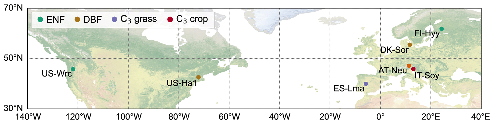
Figure 2Locations of the seven studied sites. Sites sharing the same plant function type are represented with consistent colors. The background map corresponds to the “Nature Earth I” map (https://www.naturalearthdata.com, last access: November 2023). ENF and DBF denote evergreen needleleaf forest and deciduous broadleaf forest, respectively.
Table 1Site characteristics. Site identification includes the country initials and a three-letter name for each site. Locations of the sites are provided by the latitude (Lat) and longitude (Long). PFTs covered by the sites are evergreen needleleaf forest (ENF), deciduous broadleaf forest (DBF), C3 grass, and C3 crop. Soil textures covered by the sites are sandy loam, slit loam, and loam.
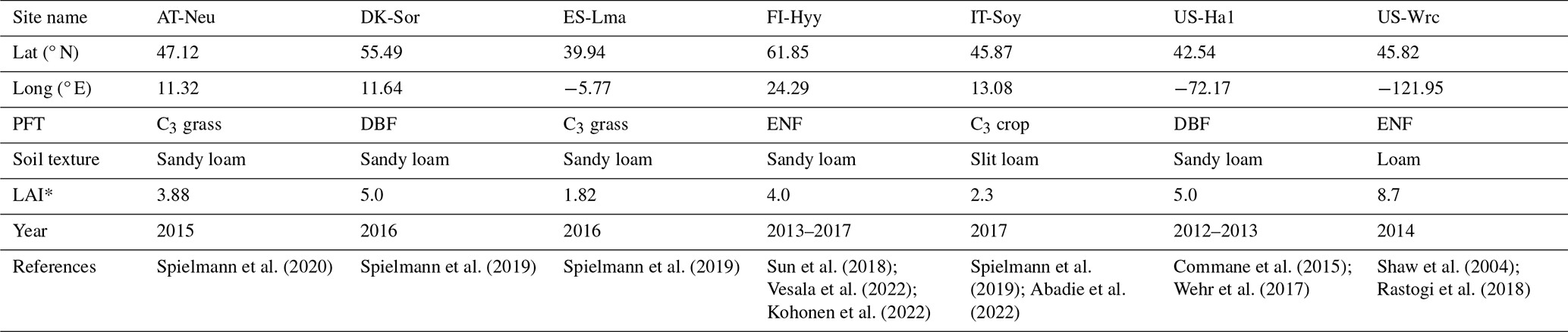
* Mean one-sided LAI (m2 m−2) during the experimental period.
2.4 Data
NUCAS was driven by several temporally and spatially variant and invariant datasets. The CO2 and COS mole fractions in the bulk air were assumed to be spatially invariant over the globe and to vary annually. The CO2 mole fraction data in this study are taken from the Global Monitoring Laboratory (https://gml.noaa.gov/ccgg/trends/global.html, last access: July 2022). For the COS mole fraction, the average of the COS mole fraction observations from sites SPO (South Pole) and MLO (Mauna Loa, United States) was utilized to drive the model, and the data are publicly available online at https://gml.noaa.gov/hats/gases/OCS.html (last access: July 2022). The other input data include a remotely sensed LAI dataset, a meteorological dataset, and a soil dataset. Additionally, in order to conduct data assimilation experiments and to evaluate the effectiveness of the assimilation of COS fluxes, field observations including the ecosystem-scale (eddy-covariance or gradient-based) COS flux, GPP, sensible heat (H), ET, and SWC collected at the sites were used.
2.4.1 LAI dataset
The LAI dataset used here comprises the GLOBMAP global leaf area index product (Version 3) (see GLOBMAP global leaf area index since 1981; Zenodo (https://doi.org/10.5281/zenodo.4700264, Liu et al., 2021)), the Global Land Surface Satellite (GLASS) LAI product (Version 3) (acquired from https://doi.org/10.12041/geodata.GLASS_LAI_MODIS(0.05 D).ver1.dbTS1, Xiao et al., 2016), and the level-4 MODIS global LAI product (see LP DAAC – MOD15A2H (https://doi.org/10.5067/MODIS/MOD15A2H.006, Myneni et al., 2015)). The GLOBMAP LAI product quantifies leaf area index at a spatial resolution of 8 × 8 km and a temporal resolution of 8 d (Liu et al., 2012). The GLASS LAI product is generated every 8 d at a spatial resolution of 1 × 1 km (Xiao et al., 2016), and the MODIS LAI is an 8 d composite dataset with 500 × 500 m pixel size. As a default, we used GLOBMAP products for assimilation experiments as much as possible given their good performance in the BEPS applications to various cases (Chen et al., 2019). The GLASS and MODIS LAI products were used to investigate the effect of the LAI products on the parameter optimization results. Also, according to Spielmann et al. (2019a), the GLOBMAP product had considerably underestimated the LAI at the DK-Sor site in June 2016, and we noticed it was not consistent with the vegetation phenology at ES-Lma in May 2016. Therefore, GLASS LAI was used at these two sites, and the GLOBMAP product was used at the remaining five sites. In addition, the 8 d temporal resolution of the LAI data was interpolated into daily values using the nearest neighbor method.
2.4.2 Meteorological dataset
Standard hourly meteorological data were inputted into BEPS, including air temperature at 2 m, shortwave radiation, precipitation, relative humidity, and wind speed, taken from the FLUXNET database (for sites AT-Neu, DK-Sor, ES-Lma, FI-Hyy, and US-Ha1; see https://fluxnet.org, last access: June 2022), the AmeriFlux database (for sites US-Ha1 and US-Wrc; see https://ameriflux.lbl.gov, last access: June 2022), and the ERA5 dataset (for sites AT-Neu, IT-Soy, and US-Ha1; see https://doi.org/10.24381/cds.adbb2d47, Hersbach et al., 2023), respectively. Since the experiments were conducted at the site scale, we used as far as possible the FLUXNET and AmeriFlux data, which contain information about the downscaling of meteorological variables of the ERA-Interim reanalysis data product, and supplemented them with ERA5 reanalysis data (Pastorello et al., 2020). Although AT-Neu is a FLUXNET site, its FLUXNET meteorological data are only available for the years 2002–2012, while the measurement of COS was performed in 2015. Therefore, we first performed a linear fit of its ERA5-Land data and FLUXNET meteorological data for 2002–2012 and then corrected the ERA5 data for 2015 with the fitted parameters to obtain downscaling information for the meteorological variables. Additionally, for US-Ha1, we used the FLUXNET data in 2012 and the AmeriFlux data and ERA5 shortwave radiation data in 2013 to drive the BEPS model due to the absence of FLUXNET data in 2013 and the lack of shortwave radiation data of AmeriFlux.
2.4.3 Assimilation and evaluation datasets
The hourly ecosystem-scale COS flux observations were used to perform data assimilation experiments and to evaluate the assimilation results. They were taken from existing studies (listed in Table 1) and were available for at least 1 month. Most of the ecosystem COS flux observations were obtained using the eddy-covariance (EC) technique, with the exception of US-Ha1 and US-Wrc, where the COS fluxes were derived with the gradient-based approach (Baldocchi, 2003; Wu et al., 2015; Kohonen et al., 2020). The COS soil flux measurements were collected using soil chambers, except at US-Ha1, where the gradient-based approach was used. Detailed information about the COS measurements can be found in the publications listed in Table 1. Specifically, only the measured ecosystem COS fluxes of FI-Hyy (Vesala et al., 2022) were utilized in this study.
US-Wrc utilizes the gradient-based approach to measure COS ecosystem flux (Rastogi et al., 2018a). However, available data are limited to only COS concentration measurements and lack other parameters required; therefore this site risks introducing biases. Hence, a bias correction scheme was implemented to match the simulated and estimated ecosystem-scale COS fluxes for US-Wrc. The objectives of this correction scheme are to obviate the need for accurate values of parameters relevant for COS flux calculations and to retain as much useful information from the COS concentration measurements as possible (Leung et al., 1999; Scholze et al., 2016). This was done by using the mean () and standard deviation (σM) of the simulated COS flux to correct the COS flux observations (O):
where and σO are the mean and standard deviation of the observed COS flux series. F is the corrected observed COS flux, and the COS simulations were calculated using the prior parameters for the time period corresponding to the COS flux observations. The standard deviation of the ecosystem COS fluxes within 24 h around each observation was calculated as an estimate of the observation uncertainty. For the case where there are no other observations within the surrounding 24 h, the uncertainty was taken as the mean of the estimated uncertainties of the whole observation series.
Due to the coupling between leaf exchange of COS, CO2 and H2O, GPP, and ET data are selected to evaluate the model performance of COS assimilation in this study. In addition, we further explored the ability of COS to constrain H simulations, since the transpiration contributes to a decrease in temperature within the leaf (Gates, 1968; Konarska et al., 2016), and the leaf–air temperature gradient is a key control factor of H (Monteith and Unsworth, 2013; Dong et al., 2017). Moreover, SWC is used in model evaluation because it plays a key role in modeling FCOS,biotic (as shown in Eq. 9) and because the water dissipated in transpiration originates from the soil (Berry et al., 2016). More detail will be provided in the Discussion (Sect. 4.3).
These data were taken from FLUXNET (DK-Sor, ES-Lma, FI-Hyy, and US-Ha1), AmeriFlux (US-Ha1 and US-Wrc), existing studies (Spielmann et al., 2020a, 2019a, and Rastogi et al., 2018a), and SMEAR (https://smear.avaa.csc.fi/, last access: May 2024). As only CO2 turbulent flux (FC) data are available for US-Ha1 in 2013 and only net ecosystem exchange (NEE) data are available for IT-Soy, a night flux partitioning model was used to estimate ecosystem respiration (Reco) and thus to calculate GPP (Reichstein et al., 2005). The model assumes that nighttime NEE represents ecosystem respiration and thus partitions FC or NEE into GPP and Reco based on the semi-empirical models of respiration, which use air temperature as a driver (Lloyd and Taylor, 1994; Lasslop et al., 2012). Since ET observations are only available from FI-Hyy at https://smear.avaa.csc.fi/ (last access: May 2024), ET is derived from latent heat (LE) as the ratio of LE to the latent heat of vaporization (Lw) (Pastorello et al., 2020). In this study, we use air temperature as a driver to calculate Lw and subsequently ET (Bolton, 1980).
We hereby note that only the comparisons of COS and GPP results before and after assimilation are presented in the main text, while the evaluations of the simulated ET (Figs. S3 and S4), H (Figs. S5 and S6), and SWC (Fig. S7) are included in the Supplement.
2.5 Experimental design
Three groups of data assimilation experiments were conducted in this study: (1) 14 model-based twin experiments were performed to investigate the ability of NUCAS to assimilate COS fluxes in different scenarios; (2) 13 single-site assimilation experiments were conducted at all seven sites to obtain the site-specific posterior parameters and the corresponding posterior model outputs based on COS flux observations; and (3) 1 two-site assimilation experiment was carried out to refine one set of parameters over two sites simultaneously and to simulate the corresponding model outputs. Prior simulations using default parameters were also performed in order to investigate the effect of the COS flux assimilation. Moreover, due to the limitation of the COS observations, all of these experiments were conducted in a 1-month time window at the peak of the growing season. Detailed information of these experiments is described in the following.
2.5.1 Twin experiment
Model-based twin experiments were performed to investigate the model performance of the data assimilation (Irrgang et al., 2017) at all seven sites considering single-site and two-site scenarios. In each twin experiment, we first created a pseudo-observation sequence by NUCAS using the prior parameters. The pseudo-observation time series included the prior simulated ecosystem COS fluxes with its uncertainties, and the latter were estimated as the standard deviation of the prior simulated COS fluxes within 24 h around each simulation. Then, a given perturbation ratio was applied to the prior parameters vector as a starting point for the interactive adjustment of parameter values to match the COS flux pseudo-observations. The effectiveness of the data assimilation methodology of NUCAS can be validated if it successfully restores the control parameters from the pseudo-observations. As a gradient-based optimization algorithm is used in NUCAS to tune the control parameters and minimize the cost function, the changes of cost function and gradient over assimilation processes can also be used to verify the assimilation performance of the system. In this work, a total of 14 twin experiments were conducted, including 13 single-site twin experiments and 1 two-site twin experiment. Regarding the uncertainty of parameters, a perturbation size of 0.2 was utilized in all of the twin experiments.
2.5.2 Real data assimilation experiment
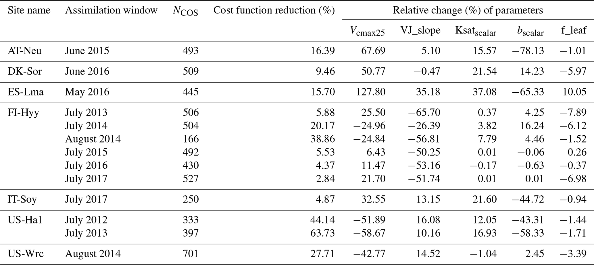
After the ability of NUCAS to assimilate COS fluxes was confirmed by twin experiments, the system was then utilized to conduct data assimilation experiments with real COS observations under single-site and two-site conditions to optimize the control parameters and state variables of this model, and the evaluation dataset was used to test the posterior simulations of the state variables. For the single-site case, a total of 13 data assimilation experiments were conducted at all sites to investigate the assimilation effect of COS flux on optimizing key ecosystem variables. Detailed information about these single-site experiments is shown in Table 2.
Table 2The configuration and the relative changes (%) of the parameters for each single-site assimilation experiment. The cost function reduction of each experiment is indicated by the reduction rate between the initial value of the cost function (Jinitial) and the final value of the cost function (Jfinal), defined as , and NCOS denotes the number of ecosystem COS flux observations.
Single-site assimilation can fully account for the site-specific information and thus achieve accurate calibration. However, this assimilation approach often yields a range of different model parameters between sites. For large-scale model simulations, only one set of accurate and generalized model parameters is required (Salmon et al., 2022). Thus, it is necessary to conduct a two-site assimilation experiment that can assimilate COS observations from two sites simultaneously. Although both DK-Sor and US-Ha1 are dominated by deciduous broadleaved forest and both AT-Neu and ES-Lma are dominated by C3 grass, none of the COS flux observations from these two PFTs overlap in observation time. We therefore selected FI-Hyy and US-Wrc, which are both dominated by evergreen needleleaf forest, and conducted a two-site assimilation experiment with a 1-month assimilation window in August 2014.
2.6 Model evaluation
For the purpose of demonstrating the process of the control parameter vector being continuously adjusted in the normalized parameter space in a twin experiment and quantifying the deviation of the current control vector from the prior, the distance (Dx) between the parameter vector and the prior parameter vector was calculated.
where i denotes the ith parameter in the parameter vectors and n denotes the number of parameters in the parameter vector and takes a value of 76.
With the aim of evaluating the performance of NUCAS in the real data assimilation experiments, we re-ran the model to obtain the posterior model outputs based on the posterior model parameters. Typical statistical metrics including mean bias (MB), root-mean-square error (RMSE), and coefficient of determination (R2) are used to measure the difference between the simulations and in situ observations. They were calculated as
where Mi denotes the simulation corresponding to the ith observation Oi and N is the total number of observations.
Additionally, in order to investigate the sensitivity of COS assimilation to the model parameters, we also calculated the sensitivity index (SI) for each parameter at the prior value based on the sensitivity information provided by the adjoint model. The SI of ith parameter x(i) of the parameter vector x was calculated as
where denotes the norm of the sensitivity vector of the cost function to the model parameters.
3.1 Twin experiments
After averaging about 18 and 13 evaluations of the cost function and its gradients, each of the twin experiments was successfully performed. Details of these twin experiments are shown in Table S5. In summary, during those assimilations, the cost function values were substantially reduced by more than 13 orders of magnitude from greater than 50.75 to less than , and the respective gradient values were also reduced from greater than 38.81 to less than , which verified the ability of the data assimilation algorithm to correctly complete the assimilation.
The relative changes of the parameters with respect to the prior values at the ends of the experiments are reported in Table S5, along with the initial values (Dinitial) and the final values (Dfinal) of Dx. Results show that the relative differences of these parameters from the “true” values reached exceedingly small values at the ends of twin experiments, with the maximum of the absolute values of the relative changes below . Dx was also reduced to nearly zero, where the maximum value was below , which indicates that all parameters in the control parameter vectors were almost fully recovered from the pseudo-observations. In conclusion, these results demonstrate that NUCAS has excellent data assimilation capability under various scenarios and can effectively perform iterative computations to achieve reliable parameter optimization.
3.2 Single-site assimilation
With an average of approximately 97 cost function evaluations, all of the 13 single-site experiments were performed successfully. The experiments reduced cost function values substantially, with an average cost function reduction of 19.97 % (Table 2). However, the cost function reduction of the experiment varies considerably with PFT, site, and assimilation window, ranging from 2.84 % to 63.73 %. The cost function decreased dramatically at US-Ha1, with an average decrease of 53.93 %. In contrast, at IT-Soy, the cost function reduction is only 4.87 %. With the same PFT (C3 grass), the cost function decreased by a similar degree at AT-Neu (16.39 %) and ES-Lma (15.70 %). The average cost function reduction at FI-Hyy (29.52 %) was also comparable to another evergreen needleleaf forest site, US-Wrc (27.71 %), in 2014. However, the cost function reduction of FI-Hyy varied notably from year to year. In July 2014 and August 2014, the cost function reductions were 20.17 % and 38.86 %, respectively, while in July of all other years the cost function reductions were much lower, ranging from 2.84 % to 5.88 %. Similarly to the single-site twin experiments, only five parameters have been efficiently adjusted in the single-site assimilation of real observations (Table 2).
The mean diurnal cycle and the scatterplots of observed and simulated COS fluxes are presented in Figs. 3 and S1, respectively. On average across all sites, the prior simulated and observed ecosystem COS fluxes were remarkably close, with 20.60 and 20.04 pmol m−2 s−1, respectively. However, there was substantial variability between sites and even between experiments at the same site. At ES-Lma, the prior simulated COS fluxes were greatly underestimated by 63.38 %. In contrast, the prior simulated COS fluxes were overestimated at US-Ha1, with MBs of −10.01 and −12.17 pmol m−2 s−1 in July 2012 and July 2013. In general, the MBs of COS fluxes are largely determined by the simulations and observations in the daytime due to the larger magnitude (Fig. 3). However, the model–observation differences at nighttime are also non-negligible. As shown in Fig. 3, the underestimation is particularly evident at AT-Neu, ES-Lma, and FI-Hyy.
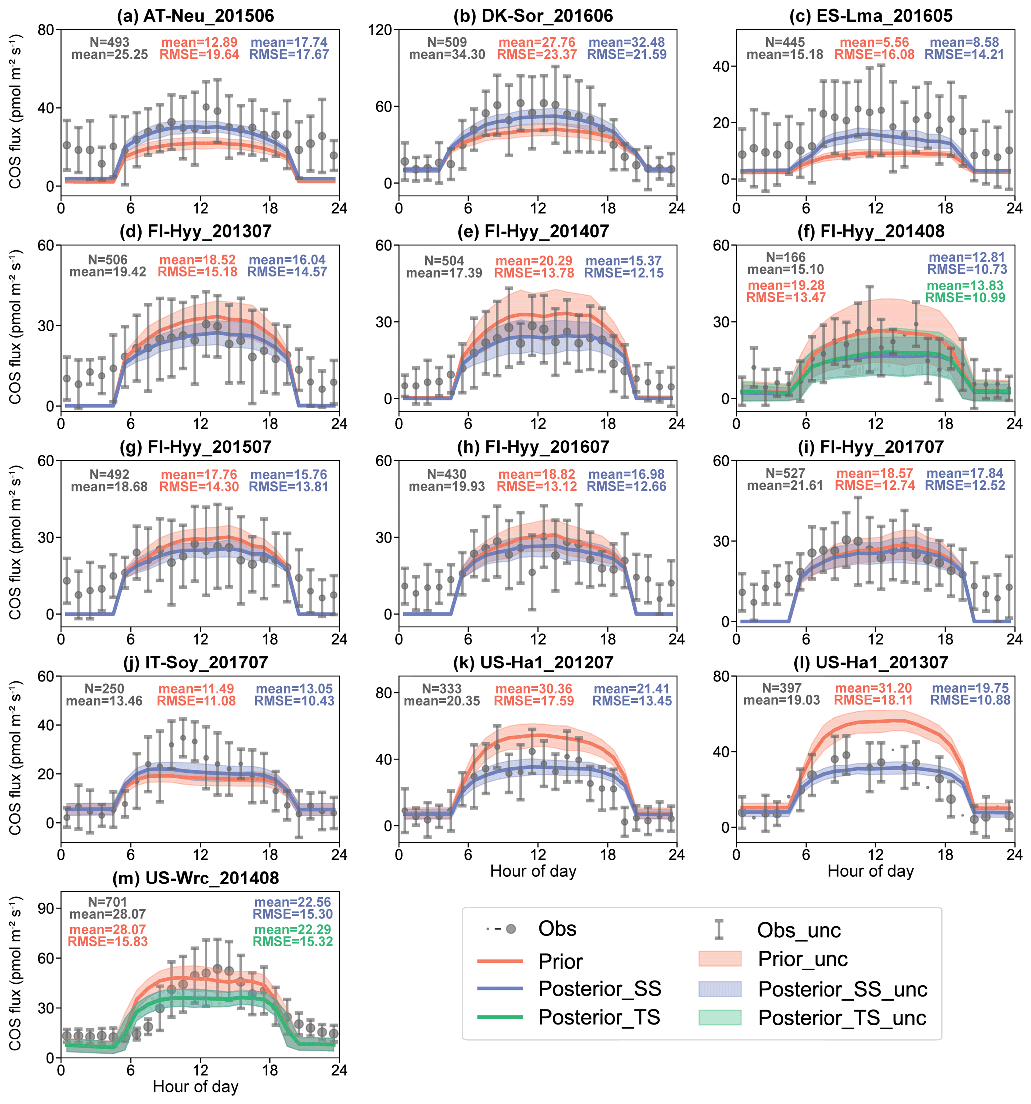
Figure 3The diurnal cycle of observed (gray) and simulated COS flux using prior parameters (red) and single-site (blue) and two-site (green) posterior parameters. The size of the circle indicates the number of observations (ranging from 1 to 31) within each circle, and the error bars depict the standard deviations in the mean of observations from the variability within each circle if the number of corresponding observations is greater than 3. Lines connect the mean values of simulations, and pale bands depict the standard deviation in the mean of simulations from the variability within each bin.
After the single-site optimizations, both the daily variation and the diurnal cycle of COS simulations were improved. This was reflected in the reduction of the mean RMSE between the simulated and observed COS fluxes from 15.71 pmol m−2 s−1 in the prior case to 13.84 pmol m−2 s−1 in the posterior case. The RMSEs were also reduced in all single-site experiments. Moreover, the assimilation of COS fluxes also effectively corrected the bias between prior simulations and observations, with the mean absolute MB decreased from 5.06 to 3.15 pmol m−2 s−1. In contrast, R2 remained almost unchanged by the optimizations, with its mean value of 0.30 in both the prior and the posterior cases. Our results also showcase that the model–observation differences in COS fluxes were effectively reduced during the daytime. However, the remarkable differences between COS flux observations and simulations at nighttime are not effectively corrected in a number of assimilation experiments (i.e., the experiment conducted at FI-Hyy in July 2013; see Fig. 3d).
3.3 Two-site assimilation
FI-Hyy and US-Wrc have different soil textures: sandy loam and loam, respectively. In the two-site assimilation experiment, NUCAS accounted for this difference appropriately and successfully minimized the cost function from 499.56 to 358.81 after 70 evaluations of cost function. The cost function reduction for the experiment has a value of 28.17 %, comparable to the cost function reductions for corresponding single-site assimilation experiments at FI-Hyy and US-Wrc (38.86 % and 27.71 %). Furthermore, corresponding to these two soil textures, the texture-dependent parameters Ksatscalar and bscalar yielded two different posterior parameter values, respectively, so that a total of seven parameters were optimized in the two-site experiment (Table 3). It can be seen that the two-site optimized results of Vcmax25, VJ_slope, and f_leaf are similar to those of the single-site optimized results at US-Wrc, as most of the observations of the two-site experiment originated from US-Wrc. As for the texture-dependent parameters, they had the same signs and comparable magnitudes of the adjustments as those of the corresponding single-site experiment at FI-Hyy and were minutely adjusted at US-Wrc as in the corresponding single-site experiment. Overall, both the cost function reduction and the parameter optimization results of the two-site assimilation experiments were similar to the corresponding single-site experiments, demonstrating the ability of NUCAS to correctly perform joint data assimilation from COS observations at two sites simultaneously.
Table 3The configuration and the relative changes (%) of the parameters for the two-site assimilation experiment at FI-Hyy and US-Wrc. NCOS denotes the total number of ecosystem COS flux observations.
The posterior simulations of COS flux using the two-site posterior parameters also demonstrated the ability of NUCAS to correctly assimilate two-site COS fluxes simultaneously (Figs. 3 and S1). As shown in Figs. 3f and 3m, the prior COS simulations for both the FI-Hyy site and US-Wrc site were overestimated in the daytime compared to the observations. After the two-site COS assimilation, the discrepancies between COS simulations and observations were reduced in both FI-Hyy and US-Wrc, with RMSE reductions of 18.42 % and 3.23 %, achieving similar results to the simulations using the single-site posterior parameters.
3.4 Parameter change
There are five parameters that were adjusted during the assimilation of COS flux observations by NUCAS, whether in twin, single-site, or two-site experiments. They are the maximum carboxylation rate at 25 °C (Vcmax25), the ratio of Vcmax to the maximum electron transport rate Jmax (VJ_slope), the scaling factor (Ksatscalar and bscalar) of saturated hydraulic conductivity (Ksat) and the Campbell parameter (b), and the ratio of PAR to shortwave radiation (f_leaf). These parameters are strongly linked to the COS exchange processes, and it is therefore reasonable that they could be optimized by the assimilation of COS flux. Furthermore, these parameters are also closely linked to processes such as photosynthesis, transpiration, and soil water transport; therefore, the assimilation of COS flux holds the promise of improving the simulation of GPP, ET, H, and SWC.
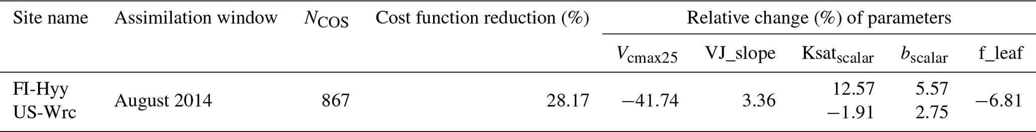
In both the single-site and the two-site experiments, Vcmax25 was considerably adjusted, with average absolute relative changes of 42.08 % and 41.74 %, respectively (Fig. 4a). VJ_slope and bscalar also varied greatly in the single-site experiments, with mean absolute relative changes of 30.67 % and 25.55 %, respectively. However, in the two-site experiment, their mean absolute changes were much smaller at 3.36 % and 4.16 %. The relative changes of Ksatscalar are modest in both the single-site and two-site experiments, with mean absolute values of 10.61 % and 7.24 %, respectively. As for f_leaf, the average absolute relative changes are even smaller than those of Ksatscalar, at 3.67 % and 6.81 % in the single-site and two-site experiments. In addition, we found that the parameters can be tuned considerably in cases where the prior simulations are close to the observations. For example, at IT-Soy, where the prior simulations agree well with the observations and the cost function only decreases 4.87 % in the experiment, both Vcmax25 and bscalar were remarkably tuned, with relative changes of 32.55 % and −44.72 %.
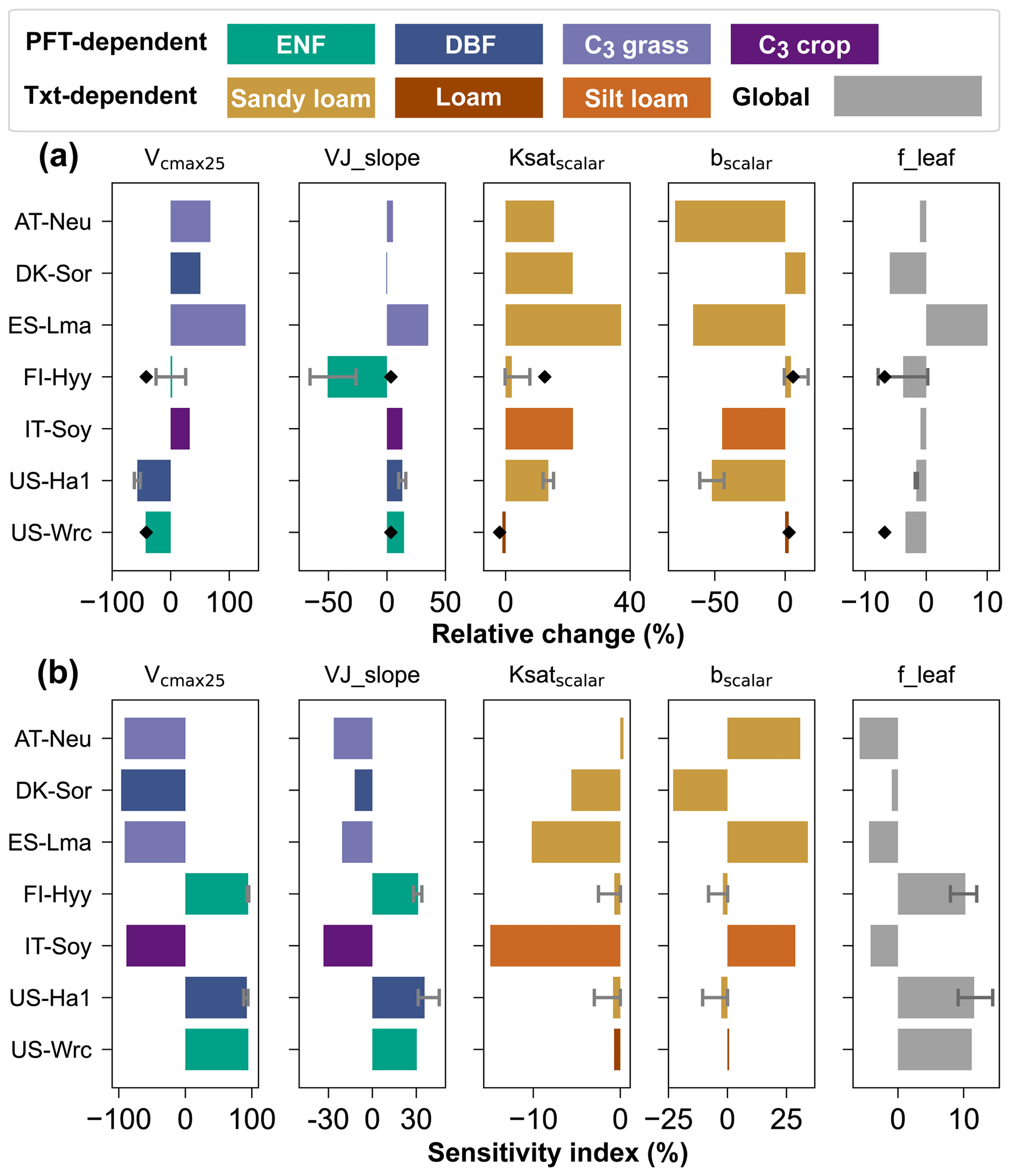
Figure 4(a) Relative changes of parameters for single-site experiments (bars) and for the two-site experiment (diamond points). (b) Sensitivity indexes of parameters at prior values. For sites where multiple single-site experiments were conducted, the ends of the error bars and the bar indicate the maximum, minimum, and mean of the relative changes of the parameters, respectively. For those sites lacking multi-year COS observations, no error bars were plotted. The color of each bar indicates the PFT/texture (Txt).
Across all single-site experiments, there are notable differences in the results of parameter optimization, especially in Vcmax25. For the single-site experiment at US-Ha1 in July 2013, the posterior value of Vcmax25 is 55.28 % lower than the prior. In contrast, the posterior Vcmax25 is 127.80 % higher than the prior at ES-Lma. In addition to Vcmax25, the relative changes of bscalar and VJ_slope also vary considerably, ranging from −78.13 % to 16.84 % and −65.70 % to 35.18 %, respectively. On the contrary, the posterior values of f_leaf show less variability and do not differ from the prior value by more than 10.05 % (note the difference in x-axis scales).
3.5 Parameter sensitivity
The adjoint-based sensitivity analysis results of the parameters are illustrated in Fig. 4b. Our results suggest that Vcmax25 has a critical impact on the assimilation results, followed by VJ_slope. With absolute SIs ranging from 87.76 % to 96.41 %, the mean absolute SI of Vcmax25 is about 3 times that of VJ_slope, which is 29.71 %. In contrast, the average absolute SIs of bscalar, f_leaf, and Ksatscalar are much lower, with 11.54 %, 8.95 % and 3.05 %, respectively.
Unlike the great variability in the posterior Vcmax25 and VJ_slope, the SIs of these two parameters are stable, especially at the same site. At US-Ha1, for example, the differences between the SIs of Vcmax25 and VJ_slope in its two experiments were all smaller than 3.05 %. Furthermore, Vcmax25 has the smallest magnitude of variation in SIs among the five parameters, with the standard deviation of the SIs being 2.62 %, despite the fact that its SIs are of a much larger order of magnitude. With the SIs ranging from 12.05 % to 45.71 % and 0.94 % to 14.43 %, VJ_slope and f_leaf also play important roles in the modeling of COS. As for Ksatscalar and bscalar, their SIs varied considerably across sites and even across experiments at the same site. For example, the absolute SIs of bscalar are as high as 30.80 % and 34.04 % at the C3 grass sites AT-Neu and ES-Lma, respectively. On the contrary, the mean absolute SI of bscalar is only 2.59 % at FI-Hyy. However, the absolute SIs of bscalar at FI-Hyy vary considerably across the experiments, ranging from 0.06 % to 10.46 %.
Our results also suggest that f_leaf tends to play a more important role in the COS assimilation at the forest sites (including FI-Hyy, US-Ha1, and US-Wrc but not DK-Sor) compared to the sites with low-stature vegetation type (AT-Neu, ES-Lma, and IT-Soy), with the mean absolute SIs about 2 times those of the latter. With a mean absolute SI of 93.44 %, Vcmax25 is also observed to be more sensitive at the forest sites. Specifically, the largest SI of Vcmax25 was observed at DK-Sor, while the SIs of VJ_slope and f_leaf of DK-Sor are noticeably lower than those of other sites, at 12.05 % and 0.94 %, respectively.
3.6 Comparison and evaluation of simulated GPP
For single-site experiments, both the prior and posterior GPP simulations performed well in modeling the daily variation and diurnal cycle of GPP, with mean R2 values of 0.83 and 0.81, respectively (Figs. 5 and S2). The discrepancy between GPP simulations and observations was substantially reduced by the assimilation of COS, from a mean RMSE of 6.71 umol m−2 s−1 in the prior case to 5.02 umol m−2 s−1 in the posterior case. Similarly to COS, the mean of the prior simulated GPP is also generally larger than that of the observed GPP. With the assimilation of COS, the bias between the observed and simulated GPP was effectively corrected, with the reduction in mean absolute MB from 3.83 to 2.40 umol m−2 s−1.
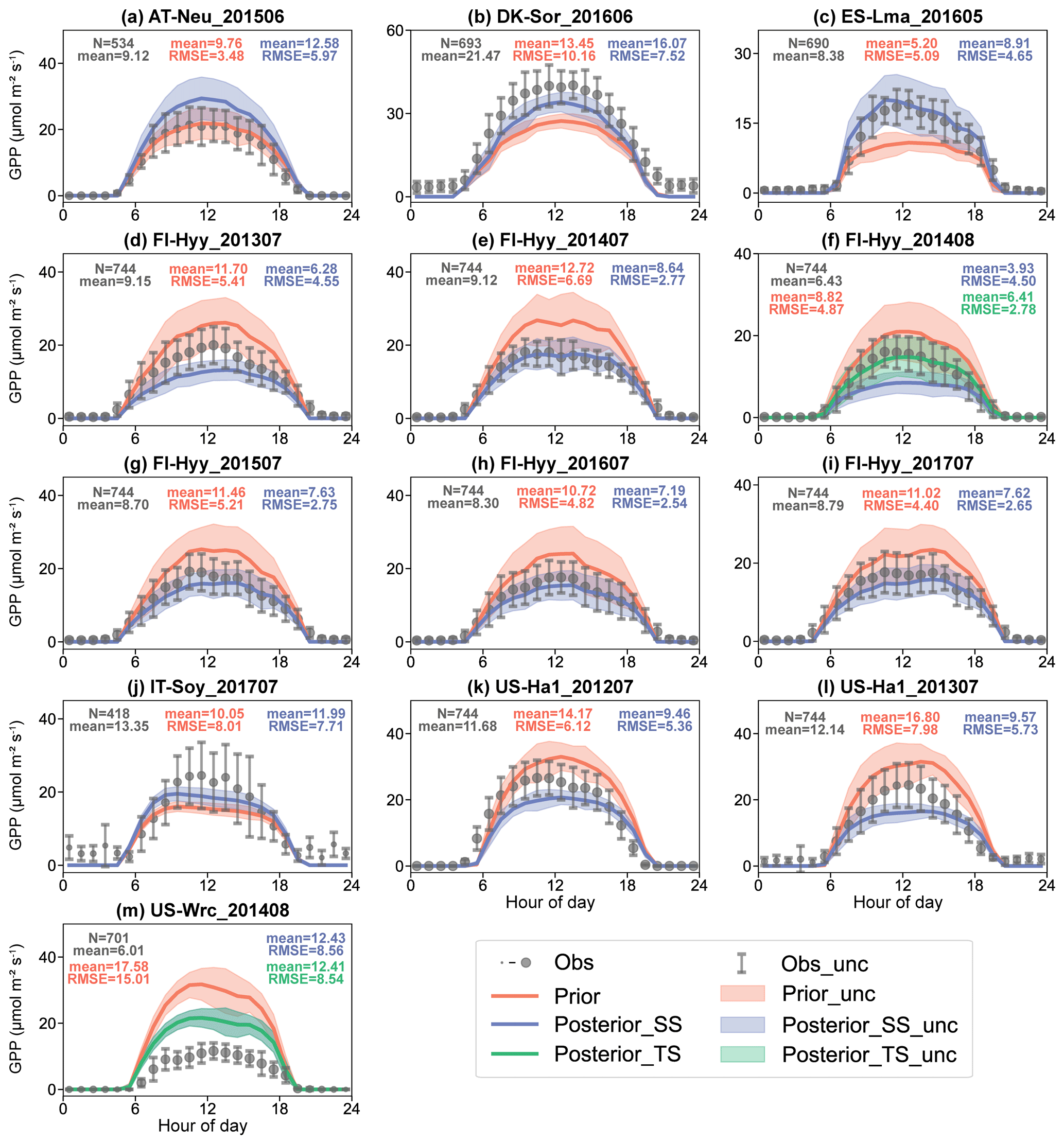
Figure 5The diurnal cycle of observed (gray) and simulated GPP using prior parameters (red) and single-site (blue) and two-site (green) posterior parameters. The size of the circle indicates the number of observations within each circle (ranging from 1 to 31), and the error bars depict the standard deviations in the mean of observations from the variability within each circle. Lines connect the mean values of simulations, and pale bands depict the standard deviation in the mean of simulations from the variability within each bin.
In general, the GPP performance was improved for most of the single-site experiments (12 of 13), with RMSE reductions ranging from 3.81 % to 58.56 %. Across all single-site experiments performed at evergreen needleleaf forest sites, the posterior GPP simulations were remarkably improved, with an averaged RMSE reduction of 37.05 %. At the deciduous broadleaf forest sites (DK-Sor and US-Ha1), the posterior simulated GPP also achieved a better fit with the GPP derived from EC observations, with an averaged RMSE reduction of 22.16 %. However, for experiments conducted on low-stature vegetation types (including C3 grass and C3 crop), the assimilation of COS is less effective in constraining the modeled GPP. At ES-Lma and IT-Soy, the RMSEs of the posterior simulated GPP are slightly lower than those of the prior, with reduction ratios of 8.60 % and 3.81 %, respectively. At AT-Neu, the assimilation of COS observations shifted the GPP simulations away from the GPP derived from EC observations, with the RMSE increasing from 3.48 to 5.97 umol m−2 s−1 (Fig. 5a).
Covering different years or months, the single-site experiments performed at FI-Hyy and US-Ha1 provided an opportunity to analyze inter-annual and seasonal variations in the simulated and observed GPP. At US-Ha1, the prior simulations overestimated GPP in both July 2012 and July 2013 by 21.26 % and 38.41 %, respectively. With the assimilation of COS, the modeled COS exhibited substantial decreases. In parallel, the model–observation difference in GPP also reduced by 12.36 % and 28.10 %, respectively. However, the posterior simulated GPP appeared to be underestimated by 20.08 %. At FI-Hyy, a total of six single-site experiments were conducted between 2013 and 2017, five of them in July and one in August 2014. The observed GPP shows little inter-annual variation in July from 2013 to 2017, with the mean ranging from 8.30 to 9.15 umol m−2 s−1. In August 2014, the GPP observations were noticeably lower than that in July, with a mean of 6.43 umol m−2 s−1. As for simulations, the model tends to overestimate GPP, with MBs ranging from 2.24 to 3.59 umol m−2 s−1. After the assimilation of COS, the overestimation of the COS simulation for FI-Hyy was effectively corrected, with mean absolute MBs of 1.53 umol m−2 s−1. However, with a low SWC in August 2014, the prior simulated COS was obviously overestimated by 37.04 %, which led to remarkable downward adjustments of Vcmax25 and VJ_slope. Thus, the simulated GPP was also markedly downgraded by 55.38 % in August 2014, ultimately resulting in the underestimation of the single-site posterior simulated GPP (Fig. 5f).
In the two-site experiment, the model–observation differences in GPP for both FI-Hyy and US-Wrc were reduced by the assimilation of COS (Fig. 5f and m), with RMSE reductions of 42.96 % and 43.11 %, respectively. These RMSE reductions are even higher than those in the corresponding single-site experiments, by 35.21 % for FI-Hyy and 0.13 % for US-Wrc. These results suggest that simultaneous assimilation using COS observations from two sites can also improve GPP simulations, and the assimilation can be more robust than the single-site assimilation because the possibility of overfitting local noise is reduced.
Overall, the assimilation of ecosystem COS fluxes improved the simulation of GPP both in single-site experiments and in the two-site experiment. However, the assimilation effects vary considerably for different sites and even for different periods within the same site. Our results suggest the assimilation of COS is able to provide strong constraint to the modeling of GPP at forest sites, with an average RMSE reduction of 32.58 %. In contrast, at the sites with low-stature vegetation type (including C3 grass and C3 crop), the assimilation of COS is less effective in constraining the GPP simulations.
4.1 Parameter changes
As mentioned before, our results show Vcmax25 was tuned the most in both the single-site experiments and the two-site experiment, followed by VJ_slope and bscalar. This is because COS plant fluxes are much larger than COS fluxes of soil in general (Whelan et al., 2016, 2018; Spielmann et al., 2019a; Kooijmans et al., 2021; Ma et al., 2021; Maignan et al., 2021; Remaud et al., 2022) and because the soil-hydrology-related parameters cannot directly influence the COS plant uptake. Therefore, the assimilation of the COS flux mainly changed the parameters related to COS plant uptake rather than texture-dependent parameters that relate to soil COS flux to minimize the cost function. However, the adjustment of soil-hydrology-related parameters should not be neglected as well, as they play an important role in minimizing the discrepancy between COS simulations and observations.
As shown in Fig. 3, the prior simulations underestimated COS fluxes at nighttime for many sites, e.g., FI-Hyy. On the one hand, this is due to the substantial gap between current modeled COS soil fluxes and observations (Whelan et al., 2022). On the other hand, this also stems from the fact that the nighttime stomatal conductance was set to a low and constant value (1 mmol m−2 s−1) in the BEPS model. As a result, the discrepancy between nighttime ecosystem COS simulations and observations could not be reduced by adjusting photosynthesis-related parameters to have an effect on stomatal conductance modeling. Thus, soil-hydrology-related parameters were adjusted to compensate for the differences in both soil and plant components simultaneously. In this study, the COS soil model proposed by Whelan et al. (2016, 2022) was utilized, in which the optimal SWC for soil COS biotic uptake was set to 12.5 % for grass. Such an optimal SWC value is much lower than the prior simulated SWC, as shown in Fig. S7a and c. Therefore, the soil-hydrology-related parameters were considerably tuned at AT-Neu and ES-Lma, resulting in a rapid decline in the posterior SWC simulation to a level comparable to the optimum SWC. COS plant uptake is governed by the hydrolysis reaction of COS (Wohlfahrt et al., 2012), catalyzed by CA, though it can also be degraded by other photosynthetic enzymes, e.g., Rubisco (Lorimer and Pierce, 1989; Ma et al., 2021), and the reaction is not dependent on light (Stimler et al., 2011; Whelan et al., 2018). However, given that stomatal conductance is simulated from net photosynthetic rate with a modified version (Woodward et al., 1995; Ju et al., 2010) of the BB model (Ball et al., 1987) in BEPS, the adjustment of light-reaction-related parameters (VJ_slope and f_leaf) can therefore indirectly affect the simulation of COS plant uptake by influencing the calculation of stomatal conductance. According to Ryu et al. (2018), f_leaf varies little in reality and is usually between 41 % and 53 % on an annual mean scale. In our assimilation experiments, the optimized f_leaf values were distributed between 42.92 % and 51.28 %, consistent with this study. In contrast, the other light-reaction-related parameter, VJ_slope, has a much wider range of variation, with relative changes ranging from −65.70 % to 35.18 %.
We noticed remarkably different optimization results for photosynthesis-related parameters in the experiments conducted in July 2013 and July 2014 at FI-Hyy, especially for Vcmax25 and VJ_slope. In these two experiments, the difference in the relative change in both Vcmax25 and VJ_slope is more than 39 %. However, these different adjustments to the parameter set caused a similar impact on COS simulations, leading to the latter being reduced by 13.38 % and 24.22 % in July 2013 and July 2014, respectively. These results revealed the “equifinality” (Beven, 1993) of the inversion problem at hand, i.e., the fact that different combinations of parameter values can achieve a similar fit to the COS observations. Assimilation of further observational data streams is expected to reduce the level of equifinality by differentiating between such combinations of parameter values that achieve a similar fit to COS observations.
4.2 Parameter sensitivity
It has been proven that photosynthetic capacity simulated by terrestrial ecosystem models is highly sensitive to Vcmax, Jmax, and light conditions (Zaehle et al., 2005; Bonan et al., 2011; Rogers, 2014; Sargsyan et al., 2014; Koffi et al., 2015; Rogers et al., 2017). Therefore, it is expected that Vcmax25, VJ_slope, and f_leaf would markedly affect the optimization results, as these parameters ultimately have an impact on the simulation of plant COS uptake by influencing the estimation of photosynthesis capacity and stomatal conductance. Specifically, the results of Wang et al. (2004), Verbeeck et al. (2006), Staudt et al. (2010), Han et al. (2020), and Ma et al. (2022) showed that the simulated photosynthetic capacity was generally more sensitive to Jmax and light conditions than to Vcmax. However, due to the differences in the physiological mechanisms of COS plant uptake and photosynthesis, e.g., the hydrolysis reaction of COS by CA is not dependent on light, the sensitivities of the two processes with respect to the model parameters may differ considerably although they are tightly coupled. Indeed, our adjoint sensitivity results suggest that the same change in Vcmax25 is capable of influencing the assimilation results to a greater extent than a change in VJ_slope and f_leaf would. This result can be attributed to the model structure of Vcmax25 that not only affects the estimation of stomatal conductance through photosynthesis but is also used to characterize mesophyll conductance and CA activity due to their linear relationships with Vcmax (Badger and Price, 1994; Evans et al., 1994; Berry et al., 2013). In addition, such a large sensitivity to Vcmax25 also indicates the importance of accurate modeling of the apparent conductance of COS for ecosystem COS flux simulation.
As for Ksatscalar and bscalar, they also play an important role in the assimilation of COS, since the SWC simulations of BEPS are sensitive to Ksat and b (Liu et al., 2011) and SWC is the primary factor for COS soil biotic flux modeling (Whelan et al., 2016). However, as the soil COS exchange is generally much smaller than COS plant uptake (Whelan et al., 2018) and the parameter scheme provided by Whelan et al. (2022) sets different empirical parameter values (see Table S3 for details) depending on the PFTs, the SIs of Ksatscalar and bscalar differ considerably across PFTs and are overall lower than those of photosynthesis-related parameters.
In Sect. 3.5, we mentioned that the radiation-related parameter f_leaf tends to play a more essential role in the assimilation of COS at the forest sites. Similar findings by Sun et al. (2019) found that the simulated GPP was more sensitive to radiation at forested vegetation types and less sensitive at low-stature vegetation types. In particular, the simulated GPP was also found to be highly sensitive to variations in radiation at low-radiation conditions (Koffi et al., 2015).
4.3 Impacts of COS assimilation on ecosystem carbon, energy, and water cycles
Due to the physiological basis that COS is taken up by plants through the same pathway of stomatal diffusion as CO2, the assimilation of COS was expected to optimize the simulation of GPP. It was confirmed by our single-site and two-site experiments conducted in a variety of ecosystems, including evergreen needleleaf forest, deciduous broadleaf forest, C3 grass, and C3 crop. However, as it is limited by many factors, such as the observation errors of the COS fluxes, the assimilation of COS does not always improve the simulation of GPP, e.g., at AT-Neu site.
Similarly to photosynthesis, transpiration is also coupled with the COS plant uptake through stomatal conductance. The difference is that, after CO2 is transported to the chloroplast surface, it continues its journey inside the chloroplast and is eventually assimilated in the Calvin cycle (Wohlfahrt et al., 2012; Kohonen et al., 2022a). Based on the BB model, photosynthesis-related parameters only indirectly influence the calculation of stomatal conductance through photosynthesis in our model. Thus, ET was not optimized as dramatically as GPP in the assimilation of COS. In comparison, the RMSEs of GPP simulations were reduced by an average of 23.54 % as a result of the assimilation of COS, but ET was reduced by only 16.96 %. Moreover, as the transpiration rate and leaf temperature change show a linear relationship (Kümmerlen et al., 1999; Prytz et al., 2003) and surface–air temperature difference is a key control factor for sensible heat fluxes (Campbell and Norman, 2000; Arya, 2001; Jiang et al., 2022), the optimization for transpiration can therefore improve the simulation of leaf temperature and consequently improve the simulation of sensible heat flux.
Driven by the difference in water potential between the atmosphere and the substomatal cavity (Manzoni et al., 2013), the water is taken up by the roots, flows through the xylem, and exits through the leaf stomata to the atmosphere in the soil–plant–atmosphere continuum via evapotranspiration (Daly et al., 2004). Thus, when plants transpire, the water potential next to the roots decreases, driving water from bulk soil towards roots (Carminati et al., 2010) and reducing soil moisture. Certainly, soil moisture dynamics are also influenced by soil evaporation and leakage during inter-storm periods under ideal conditions (Daly et al., 2004). However, studies have shown that transpiration represents 80 % to 90 % of terrestrial evapotranspiration (Jasechko et al., 2013) and that evaporation is typically a small fraction of transpiration for well-vegetated ecosystems (Scholes and Walker, 1993; Daly et al., 2004). Based on current knowledge of leakage, for example, the relationship between leakage and the behavior of hydraulic conductivity (Clapp and Hornberger, 1978), extremely small adjustments of Ksat and b (i.e., with relative changes of 0.0057 % for Ksatscalar and −0.057 % for bscalar in July 2015 at FI-Hyy) hardly caused any change in leakage. Therefore, our results indicate that the assimilation of COS can not only markedly improve the modeling of stomatal conductance and transpiration, but it can also ultimately impact SWC predictions. However, our results also show that there are obvious discrepancies between the ecosystem COS flux simulations and observations and that discrepancies cannot be effectively reduced by the adjustment of the photosynthesis-related parameters due to the simplification of BEPS for nighttime stomatal conductance modeling. As a result, it was also observed that the soil-hydrology-related parameters were drastically adjusted to minimize the discrepancy of COS simulations and observations, which instead biased the SWC simulations away from observations, for example, as shown in Figs. S7a and c.
4.4 Impacts of leaf area index data on parameter optimization
As essential input data of the BEPS model, LAI products have been demonstrated to be a source of uncertainty in the simulation of carbon and water fluxes (Liu et al., 2018). Therefore, it is necessary to investigate the influence of LAI on our parameter optimization results, as the LAI is directly related to the simulation of COS, and the discrepancy between COS simulations and COS observations is an essential part of the cost function. Here we collected three widely used satellite-derived LAI products (GLOBMAP, GLASS, and MODIS) and the means of the in situ LAI during the growing seasons or during the COS measurement periods for these sites (see Table 1). These in situ LAI means were used to drive the BEPS model along with the other three satellite-derived LAI products, with the assumption that they are representative of the LAI values during the assimilation periods. The configurations of these assimilation experiments were the same as those listed in Table 2 so that a total of 52 single-site experiments were conducted. All experiments were successfully performed, and the results are shown in Figs. 6 and S8.
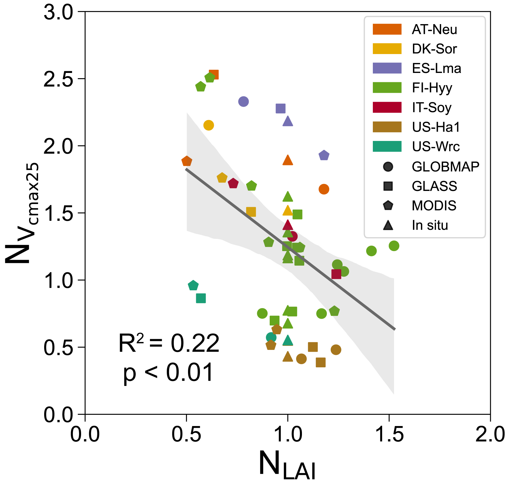
Figure 6Influence of LAI on the posterior Vcmax25 obtained by the single-site experiments conducted at seven sites and driven by four LAI datasets (GLOBMAP, GLASS, MODIS, and in situ). The posterior Vcmax25 and the LAI were represented by their normalized values, and NLAI, respectively. The posterior parameters were normalized by their prior values, and the LAI was normalized by the in situ values. The best-fit linear regression line of the posterior parameters obtained based on the satellite-derived LAI (GLOBMAP, GLASS, and MODIS) with the corresponding LAI data is shown, with the 95 % confidence interval spread around the line.
We found that the posterior Vcmax25 significantly correlated with the LAI (R2=0.22, P<0.01), while there was no apparent relationship between the optimization results of the other four parameters and the LAI. As mentioned before, the LAI is directly related to the simulation of COS and thus influences the posterior values of the parameters. Therefore, the correlations of LAI with these parameters reflect the robustness of the constraint abilities of COS assimilation with respect to them. These results suggest that the assimilation of COS is able to provide strong constraints on Vcmax25, while it constrains other parameters (VJ_slope, Ksatscalar, bscalar, and f_leaf) weakly, although they are also considerably changed by the assimilation. In conclusion, our results suggest that the uncertainty in satellite-derived LAI can not only exert large impacts on the modeling of water–carbon fluxes (Wang et al., 2021), but it is an important source of uncertainty in the parameter optimization results when performing data assimilation experiments with ecosystem models driven by LAI.
4.5 Caveats and implications
In general, we found that the assimilation of ecosystem COS fluxes can improve the model performance for GPP, ET, and H for both the single-site assimilation and the two-site assimilation. Nonetheless, there are currently limitations that affect the use of COS data for the optimization of parameters, processes, and variables related to water–carbon cycling and energy exchange in terrestrial ecosystem models.
The assimilation of COS fluxes relies on the availability and quality of field observations. As both COS plant uptake and COS soil exchange are modeled within NUCAS and the data assimilation was performed at the ecosystem scale, a large number of accurate measurements of both COS soil flux and COS plant flux are essential for COS assimilation and model evaluation. However, at present, we face a serious lack of COS measurements (Brühl et al., 2012; Wohlfahrt et al., 2012). More laboratory and field measurements are needed for better understanding of the mechanistic processes of COS. Besides, the existing COS fluxes were calculated based on different measurement methods and data processing steps, which poses considerable challenges for comparing COS flux measurements across sites. In particular, as only raw COS concentrations were provided and a correction approach was employed, the estimated COS fluxes at US-Wrc may be subject to considerable uncertainties. A standardization of the measurement and processing techniques of COS is therefore urgently needed (Kohonen et al., 2020).
In this study, the prior uncertainty of observation was estimated by the standard deviation of ecosystem COS fluxes within 24 h with the assumption of a normal distribution. However, Hollinger and Richardson (2005) suggested that flux measurement error more closely follows a double exponential than a normal distribution. Kohonen et al. (2020) showed that the overall uncertainty in the COS flux varies with the sign (uptake or release) and the magnitude of the COS flux. Furthermore, there is a lack of understanding of the prior uncertainty for certain model parameters, such as VJ_slope, which makes the uncertainty estimates subject to potentially large errors. In conclusion, we should be more careful in considering the distribution and the magnitude of the prior uncertainty of observations and parameters.
The spatial and temporal variation in atmospheric COS concentrations has a considerable influence on the COS plant uptake (Ma et al., 2021) due to the linear relationship between the two (Stimler et al., 2010). The typical seasonal amplitude of atmospheric COS concentrations is ∼ 100–200 parts per trillion (ppt) around an average of ∼ 500 ppt (Montzka et al., 2007; Kooijmans et al., 2021; Hu et al., 2021; Ma et al., 2021; Belviso et al., 2022). However, in NUCAS, COS mole fractions in the bulk air are currently assumed to be spatially invariant over the globe and to vary annually, which may introduce substantial errors into the parameter calibration. Kooijmans et al. (2021) confirmed that modifying the COS mole fractions to vary spatially and temporally markedly improved the simulation of ecosystem COS flux. Thus, we suggest taking into account the variations in COS concentration and their interaction with surface COS fluxes at high spatial and temporal resolution in order to achieve better parameter calibration.
Currently, there are still uncertainties in the simulation of COS fluxes by BEPS, particularly for nighttime COS fluxes. As the nighttime COS plant uptake is driven by stomatal conductance (Kooijmans et al., 2021), nighttime COS fluxes can therefore be used to test the accuracy of the model settings for nighttime stomatal conductance (gn). In the BEPS model, a low and constant value (1 mmol m−2 s−1) of gn was set for all PFTs. Our simulations of nighttime COS flux indicate that, in BEPS, gn is underestimated to different degrees for different sites. Similar findings by Resco De Dios et al. (2019) showed that the median gn in the global dataset was 40 mmol m−2 s−1. Therefore, the utilization of COS to directly optimize stomatal-related parameters should be investigated. Cho et al. (2023) proved the effectiveness of optimizing the minimum stomatal conductance and other parameters by the assimilation of COS. As different enzymes have different physiological characteristics, Cho et al. (2023) proposed a new temperature function for the CA enzyme and showcased the considerable difference in temperature response of enzymatic activities of CA and Rubisco, which provided valuable insights into the modeling and assimilation of COS. In addition, soil COS exchange is an important source of uncertainty in the use of COS as a carbon–water cycle tracer, since CA activity occurs in the soil as well (Kesselmeier et al., 1999; Smith et al., 1999; Ogée et al., 2016; Meredith et al., 2019). Kaisermann et al. (2018) showed that COS hydrolysis rates were linked to microbial C biomass, whilst COS production rates were linked to soil nitrogen content and mean annual precipitation (MAP). Interestingly, MAP was also suggested to be the best predictor of gn by Yu et al. (2019), who found that plants in locations with lower rainfall conditions had higher gn. Therefore, by using the global microbial C biomass, soil nitrogen content, and MAP datasets; the relationships between these variables; and the associated COS exchange processes, it is to be expected that a more accurate modeling of terrestrial ecosystem COS fluxes could be achieved, further increasing our understanding of the global COS budget and facilitating the assimilation of COS fluxes.
Over the past decades, considerable efforts have been made to obtain field observations of COS ecosystem fluxes and to describe empirically or mechanistically COS plant uptake and soil exchange, which offer the possibility of investigating the ability of assimilating ecosystem COS flux to optimize parameters and variables related to the water and carbon cycles and to energy exchange. In this study, we introduced NUCAS, a system which was developed based on the BEPS model and was designed to have the ability to assimilate ecosystem COS fluxes. In NUCAS, a resistance analog model of COS plant uptake and an empirical model of soil COS flux were embedded in the BEPS model to achieve the simulation of ecosystem COS flux, and a gradient-based 4D-Var data assimilation algorithm was implemented to optimize the internal parameters of BEPS.
A total of 14 twin experiments, 13 single-site experiments, and 1 two-site experiment covering the period from 2012 to 2017 were conducted to investigate the capability of NUCAS to assimilate COS fluxes and to optimize input parameters and simulated variables. COS flux observations from a range of ecosystems were used, including four PFTs and three soil textures. Our results show that NUCAS has the ability to optimize parameter vectors and that the assimilation of COS can constrain parameters affecting the simulation of carbon and water cycles and of energy exchange and thus effectively improve the performance of the BEPS model. We found that there is a tight link between the assimilation of COS fluxes and the optimization of ET which demonstrates the role of COS as an indicator of stomatal conductance and transpiration. The improvement of ET can further improve the model performance for H, although the propagation of the optimization effect is subject to some limitations. These results highlight the broad perspective of COS as a tracer for improving the simulation of variables related to stomatal conductance. Furthermore, we demonstrated that COS can provide a strong constraint on Vcmax25, whereas the adjustment of parameters related to the soil hydrology appears to compensate for weaknesses in the model, i.e., the nighttime stomatal conductance set in the BEPS model. We also proved the strong impact of LAI on the parameter optimization results, emphasizing the importance of developing more accurate LAI products for models driven by observed LAI. In addition, we made a number of recommendations for future improvement of the assimilation of COS. In particular, we flagged the need for more observations of COS and suggested better characterization of observational and prior parameter uncertainties, the use of varying COS concentrations, and the refinement of the model for COS fluxes of soil. Specifically, with the lack of separate COS plant and soil flux data, the ecosystem-scale COS flux observations were utilized in this study. However, we believe that assimilating the component fluxes of COS individually should be pursued in the future, as this assimilation approach would provide separate constraints on different parts of the model. We expect the observational information on the partitioning between the two flux components to provide a stronger constraint than using just their sum.
Our two-site setup constitutes a challenge for the assimilation system, the model, and the observations. In this setup, the assimilation system has to determine a parameter set that achieves a fit to the observations at both sites, and NUCAS passes this important test. It should be noted that NUCAS was designed as a platform that integrates multiple data streams to provide a consistent map of the terrestrial carbon cycle, although only ecosystem COS fluxes were used to evaluate the performance of NUCAS in this study. The two-site assimilation experiment conducted in this study gives us more confidence that the calibrated model will provide a reasonable parameter set and posterior simulation throughout the plant functional type. In other words, what we present here is a pre-requisite for applying the model and assimilation system at regional to global scales.
We noticed the optimization of model parameters faced the challenge of equifinality due to the complexity of the model and the limited observation data. However, the equifinality can be avoided by imposing additional observational constraints (Beven, 2006). Indeed, using several different data streams to simultaneously (Kaminski et al., 2012; Schürmann et al., 2016; Scholze et al., 2016; Wu et al., 2018; Scholze et al., 2019) or step-wise (Peylin et al., 2016) constrain multiple processes in the carbon cycle is becoming a focus area in carbon cycle research. Therefore, it is necessary to combine COS with other observations to constrain different ecosystem processes and/or exploit multiple constraints on the same processes in order to achieve better modeling and prediction of the ecosystem water–carbon cycle and energy exchange.
In the BEPS model, the leaf stomatal conductance to water vapor (gsw in mol m−2 s−1) is estimated using a modified version of the BB empirical model (Ball et al., 1987) following Woodward et al. (1995):
where is the intercept of the BB model, representing the minimum gsw (mol m−2 s−1); is the empirical slope parameter in the BB model (unitless); Rh is the relative humidity at the leaf surface (unitless); fw is a soil moisture stress factor describing the sensitivity of gsw to soil water availability (Ju et al., 2006); and Ca is the atmospheric CO2 concentration (µmol mol−1). The net photosynthesis rate (A) is calculated using the Farquhar model (Farquhar et al., 1980; Chen et al., 1999):
where Ai and Aj are Rubisco-limited and RuBP-limited gross photosynthetic rates (µmol m−2 s−1), respectively. Rd is leaf dark respiration (µmol m−2 s−1). Vcmax is the maximum carboxylation rate of Rubisco (µmol m−2 s−1); J is the electron transport rate (µmol m−2 s−1); Ci and Oi are the intercellular carbon dioxide (CO2) and oxygen (O2) concentrations (mol mol−1), respectively; and Kc and Ko are Michaelis–Menten constants for CO2 and O2 (mol mol−1), respectively.
The electron transport rate, J, is dependent on incident photosynthetic photon flux density (PPFD; µmol m−2 s−1) as
where Jmax is the maximum electron transport rate (µmol m−2 s−1) and I is the incident PPFD calculated from the incident shortwave radiation RSW (W m−2):
where β=4.55 is the energy–quanta conversion factor (µmol J−1) and f_leaf is the ratio of photosynthetically active radiation to the shortwave radiation (unitless).
The maximum carboxylation rate of Rubisco Vcmax was calculated according to the Arrhenius temperature function and the maximum carboxylation rate of Rubisco at 25 °C (Vcmax25). Vcmax is generally proportional to leaf nitrogen content. Considering that the fractions of both sunlit and shaded leaf areas to the total leaf area and the leaf nitrogen content vary with the depth into the canopy (L), the Vcmax values of sunlit (Vcmax,sun) and shaded (Vcmax,sh) leaves can be obtained through vertical integrations with respect to L (Chen et al., 2012):
where χn (m2 g−1) is the relative change in Vcmax to leaf nitrogen content; Nleaf (g m−2) is the leaf nitrogen content at the top of the canopy; and kn (unitless) is the leaf nitrogen content decay rate with increasing depth into the canopy, taken as 0.3. k is calculated as
where G(θ) is the projection coefficient, taken as 0.5; Ω is the clumping index; and θ is the solar zenith angle.
After Vcmax values for the representative sunlit and shaded leaves are obtained, the maximum electronic transport rate for the sunlit and shaded leaves is obtained from Medlyn et al. (1999):
The soil water availability factor fw,i in each layer i is calculated as
where fi(ψi) is a function of matrix suction ψi (m) (Zierl, 2001) and fi(Ts,i) is a function describing the effect of soil temperature (Ts,i in °C) on soil water uptake (Bonan, 1991).
To consider the variable soil water potential at different depths, the scheme of Ju et al. (2006) was employed to calculate the weight of each layer (wi) to fw:
where n is the soil layer number (five were used in this study) of the BEPS model and Ri is the root fraction in layer i, calculated as
where cdi is the cumulative depth (m) of layer i. In this study, each soil layer depth (from top to bottom) of the BEPS model is 0.05, 0.10, 0.20, 0.40, and 1.25 m, respectively.
The overall soil water availability fw is then calculated as
The hydraulic conductivity of each soil layer Ki (m s−1) is expressed as
where Ksati is the saturated hydrological conductivity of soil layer i (m s−1); SWCi is the volumetric liquid soil water content of soil layer i (m s−1); θs, i is the porosity of soil layer i (unitless); and bi is the Campbell parameter for soil layer i, determining the change rate of hydraulic conductivity with SWC (unitless). In this study, Ksati and bi are expressed as
where Ksatdf,i and bdf,i are the default values of Ksati and bi, respectively.
The source code for BEPS is publicly available at https://doi.org/10.5281/zenodo.10667005 (Wu, 2023), and the adjoint code for BEPS is available upon request from the correspondence author (mousongwu@nju.edu.cn).
Measured eddy-covariance carbonyl sulfide flux data can be found at https://doi.org/10.5281/zenodo.3993111 (Spielmann et al., 2020b) for AT-Neu; https://doi.org/10.5281/zenodo.3406990 (Spielmann et al., 2019b) for DK-Sor, ES-Lma, and IT-Soy; https://doi.org/10.5281/zenodo.6940750 (Kohonen et al., 2022b) for FI-Hyy; and from the Harvard Forest Data Archive under record HF214 (https://doi.org/10.6073/pasta/7ed7b4d1fc7ad303998e76143a3b279a; Commane et al., 2016) for US-Ha1.The raw COS concentration data of US-Wrc can be obtained at https://doi.org/10.5281/zenodo.1422820 (Rastogi et al., 2018b). The meteorological data can be obtained from the FLUXNET database (https://fluxnet.org/, last access: June 2022) for AT-Neu (https://doi.org/10.18140/FLX/1440121, Georg et al., 2020; Pastorello et al., 2020), DK-Sor (https://doi.org/10.18140/FLX/1440155, Andreas and Kim, 2020), ES-Lma (https://doi.org/10.18160/FDSD-GVRS, Migliavacca et al., 2020), FI-Hyy (https://doi.org/10.18140/FLX/1440158, Ivan et al., 2020), and US-Ha1 (https://doi.org/10.18140/FLX/1440071, Harvard University, 2020); from the AmeriFlux database (https://ameriflux.lbl.gov/, last access: June 2022) for US-Ha1 (https://doi.org/10.17190/AMF/1871137, Munger, 2022) and US-Wrc (https://doi.org/10.17190/AMF/1246114, Wharton, 2016); and from the ERA5 dataset (https://doi.org/10.24381/cds.adbb2d47; Hersbach et al., 2023) for AT-Neu, IT-Soy, and US-Ha1. The evaluation data can be obtained from the FLUXNET database for DK-Sor, ES-Lma, FI-Hyy, and US-Ha1; from the AmeriFlux database for US-Ha1 and US-Wrc; from https://doi.org/10.5281/zenodo.3993111 (Spielmann et al., 2020b) for AT-Neu; from https://smear.avaa.csc.fi/ (last access: May 2024) for FI-Hyy; from https://doi.org/10.5281/zenodo.3406990 (Spielmann et al., 2019b) for IT-Soy; and from https://doi.org/10.5281/zenodo.1422820 (Rastogi et al., 2018b) for US-Wrc. The H and LE data of AT-Neu and IT-Soy are provided by Felix M. Spielmann and Georg Wohlfahrt. The GLOBMAP LAI is available at https://doi.org/10.5281/zenodo.4700264 (Liu et al., 2021), the GLASS LAI is available at https://doi.org/10.12041/geodata.GLASS_LAI_MODIS(0.05D).ver 1.db (Xiao et al., 2016), and the MODIS LAI product is available at https://doi.org/10.5067/MODIS/MOD15A2H.006 (Myneni et al., 2015). All datasets used in this study and the model outputs are available upon request.
The supplement related to this article is available online at: https://doi.org/10.5194/gmd-17-6337-2024-supplement.
MW designed the experiments and developed the model. MV and TK developed the data assimilation layer including the adjoint code for the ecosystem model. HZ wrote the original paper and made the analysis. All authors contributed to the writing of the paper.
The contact author has declared that none of the authors has any competing interests.
Publisher’s note: Copernicus Publications remains neutral with regard to jurisdictional claims made in the text, published maps, institutional affiliations, or any other geographical representation in this paper. While Copernicus Publications makes every effort to include appropriate place names, the final responsibility lies with the authors.
We thank everyone that contributed to the collection of data. Specifically, we acknowledge Felix M. Spielmann and Georg Wohlfahrt for providing H and LE data for AT-Neu and IT-Soy. Michael Vossbeck and Thomas Kaminski thank Laurent Hascoët for supporting this activity. The authors thank the reviewers for their highly valuable comments.
This research has been supported by the National Key Research and Development Program of China (grant no. 2020YFA0607504), the National Natural Science Foundation of China (grant no. 42371486), and the Research Funds for the Frontiers Science Center for Critical Earth Material Cycling, Nanjing University (grant nos. 0209-14380115 and 0904-14380031).
This paper was edited by Yilong Wang and reviewed by Kukka-Maaria Kohonen, Michael Cartwright, and one anonymous referee.
Abadie, C., Maignan, F., Remaud, M., Ogée, J., Campbell, J. E., Whelan, M. E., Kitz, F., Spielmann, F. M., Wohlfahrt, G., Wehr, R., Sun, W., Raoult, N., Seibt, U., Hauglustaine, D., Lennartz, S. T., Belviso, S., Montagne, D., and Peylin, P.: Global modelling of soil carbonyl sulfide exchanges, Biogeosciences, 19, 2427–2463, https://doi.org/10.5194/bg-19-2427-2022, 2022.
An, X. Q., Zhai, S. X., Jin, M., Gong, S., and Wang, Y.: Development of an adjoint model of GRAPES–CUACE and its application in tracking influential haze source areas in north China, Geosci. Model Dev., 9, 2153–2165, https://doi.org/10.5194/gmd-9-2153-2016, 2016.
Andreas, I. and Kim, P.: FLUXNET2015 DK-Sor Soroe, FLUXNET2015 [data set], https://doi.org/10.18140/FLX/1440155, 2020.
Arias, P., Bellouin, N., Coppola, E., Jones, R., Krinner, G., Marotzke, J., Naik, V., Palmer, M., Plattner, G.-K., and Rogelj, J.: Climate Change 2021: The Physical Science Basis. Contribution of Working Group I to the Sixth Assessment Report of the Intergovernmental Panel on Climate Change, Technical Summary, https://www.ipcc.ch/report/ar6/wg1/ (last access: April 2023), 2021.
Arya, P. S.: Introduction to micrometeorology, Elsevier, ISBN 0080489265, 2001.
Asaf, D., Rotenberg, E., Tatarinov, F., Dicken, U., Montzka, S. A., and Yakir, D.: Ecosystem photosynthesis inferred from measurements of carbonyl sulphide flux, Nat. Geosci., 6, 186–190, 2013.
Bäck, J., Aalto, J., Henriksson, M., Hakola, H., He, Q., and Boy, M.: Chemodiversity of a Scots pine stand and implications for terpene air concentrations, Biogeosciences, 9, 689–702, https://doi.org/10.5194/bg-9-689-2012, 2012.
Badger, M. R. and Price, G. D.: The role of carbonic anhydrase in photosynthesis, Annu. Rev. Plant. Biol., 45, 369–392, 1994.
Baldocchi, D. D.: Assessing the eddy covariance technique for evaluating carbon dioxide exchange rates of ecosystems: past, present and future, Glob. Change Biol., 9, 479–492, 2003.
Ball, J. T., Woodrow, I. E., and Berry, J. A.: A Model Predicting Stomatal Conductance and its Contribution to the Control of Photosynthesis under Different Environmental Conditions, in: Progress in Photosynthesis Research: Volume 4 Proceedings of the VIIth International Congress on Photosynthesis Providence, Rhode Island, USA, 10–15 August 1986, edited by: Biggins, J., Springer Netherlands, Dordrecht, 221–224, https://doi.org/10.1007/978-94-017-0519-6_48, 1987.
Behrendt, T., Veres, P. R., Ashuri, F., Song, G., Flanz, M., Mamtimin, B., Bruse, M., Williams, J., and Meixner, F. X.: Characterisation of NO production and consumption: new insights by an improved laboratory dynamic chamber technique, Biogeosciences, 11, 5463–5492, https://doi.org/10.5194/bg-11-5463-2014, 2014.
Belviso, S., Remaud, M., Abadie, C., Maignan, F., Ramonet, M., and Peylin, P.: Ongoing Decline in the Atmospheric COS Seasonal Cycle Amplitude over Western Europe: Implications for Surface Fluxes, Atmosphere, 13, 812, https://doi.org/10.3390/atmos13050812, 2022.
Berry, J., Wolf, A., Campbell, J. E., Baker, I., Blake, N., Blake, D., Denning, A. S., Kawa, S. R., Montzka, S. A., Seibt, U., Stimler, K., Yakir, D., and Zhu, Z.: A coupled model of the global cycles of carbonyl sulfide and CO2: A possible new window on the carbon cycle, J. Geophys. Res.-Biogeo., 118, 842–852, https://doi.org/10.1002/jgrg.20068, 2013.
Berry, S. L., Farquhar, G. D., and Roderick, M. L.: Co-Evolution of Climate, Soil and Vegetation, in: Encyclopedia of Hydrological Sciences, edited by: Anderson, M. G. and McDonnell, J. J., https://doi.org/10.1002/0470848944.hsa011, 2016
Beven, K.: Prophecy, reality and uncertainty in distributed hydrological modelling, Adv. Water Resour., 16, 41–51, 1993.
Beven, K.: A manifesto for the equifinality thesis, J. Hydrol., 320, 18–36, 2006.
Bolton, D.: The computation of equivalent potential temperature, Mon. Weather Rev., 108, 1046–1053, 1980.
Bonan, G. B.: A biophysical surface energy budget analysis of soil temperature in the boreal forests of interior Alaska, Water Resour. Res., 27, 767–781, 1991.
Bonan, G. B., Lawrence, P. J., Oleson, K. W., Levis, S., Jung, M., Reichstein, M., Lawrence, D. M., and Swenson, S. C.: Improving canopy processes in the Community Land Model version 4 (CLM4) using global flux fields empirically inferred from FLUXNET data, J. Geophys. Res.-Biogeo., 116, G02014, https://doi.org/10.1029/2010JG001593, 2011.
Braendholt, A., Ibrom, A., Larsen, K. S., and Pilegaard, K.: Partitioning of ecosystem respiration in a beech forest, Agr. Forest Meteorol., 252, 88–98, 2018.
Brühl, C., Lelieveld, J., Crutzen, P. J., and Tost, H.: The role of carbonyl sulphide as a source of stratospheric sulphate aerosol and its impact on climate, Atmos. Chem. Phys., 12, 1239–1253, https://doi.org/10.5194/acp-12-1239-2012, 2012.
Campbell, G. S. and Norman, J. M.: An introduction to environmental biophysics, Springer Science & Business Media, https://doi.org/10.1007/978-1-4612-1626-1, 2000.
Campbell, J. E., Carmichael, G. R., Chai, T., Mena-Carrasco, M., Tang, Y., Blake, D., Blake, N., Vay, S. A., Collatz, G. J., and Baker, I.: Photosynthetic control of atmospheric carbonyl sulfide during the growing season, Science, 322, 1085–1088, 2008.
Carminati, A., Moradi, A. B., Vetterlein, D., Vontobel, P., Lehmann, E., Weller, U., Vogel, H.-J., and Oswald, S. E.: Dynamics of soil water content in the rhizosphere, Plant Soil, 332, 163–176, 2010.
Chen, J., Liu, J., Cihlar, J., and Goulden, M.: Daily canopy photosynthesis model through temporal and spatial scaling for remote sensing applications, Ecol. Model., 124, 99–119, 1999.
Chen, J. M., Mo, G., Pisek, J., Liu, J., Deng, F., Ishizawa, M., and Chan, D.: Effects of foliage clumping on the estimation of global terrestrial gross primary productivity, Global Biogeochem. Cy., 26, GB1019, https://doi.org/10.1029/2010GB003996, 2012.
Chen, J. M., Ju, W., Ciais, P., Viovy, N., Liu, R., Liu, Y., and Lu, X.: Vegetation structural change since 1981 significantly enhanced the terrestrial carbon sink, Nat. Commun., 10, 4259, https://doi.org/10.1038/s41467-019-12257-8, 2019.
Chen, J. M., Wang, R., Liu, Y., He, L., Croft, H., Luo, X., Wang, H., Smith, N. G., Keenan, T. F., Prentice, I. C., Zhang, Y., Ju, W., and Dong, N.: Global datasets of leaf photosynthetic capacity for ecological and earth system research, Earth Syst. Sci. Data, 14, 4077–4093, https://doi.org/10.5194/essd-14-4077-2022, 2022.
Cho, A., Kooijmans, L. M. J., Kohonen, K.-M., Wehr, R., and Krol, M. C.: Optimizing the carbonic anhydrase temperature response and stomatal conductance of carbonyl sulfide leaf uptake in the Simple Biosphere model (SiB4), Biogeosciences, 20, 2573–2594, https://doi.org/10.5194/bg-20-2573-2023, 2023.
Clapp, R. B. and Hornberger, G. M.: Empirical equations for some soil hydraulic properties, Water Resour. Res., 14, 601–604, 1978.
Commane, R., Meredith, L. K., Baker, I. T., Berry, J. A., Munger, J. W., Montzka, S. A., Templer, P. H., Juice, S. M., Zahniser, M. S., and Wofsy, S. C.: Seasonal fluxes of carbonyl sulfide in a midlatitude forest, P. Natl. Acad. Sci. USA, 112, 14162–14167, 2015.
Commane, R., Wofsy, S., and Weir, R.: Fluxes of Carbonyl Sulfide at Harvard Forest EMS Tower since 2010, ver 4, Environmental Data Initiative [data set], https://doi.org/10.6073/pasta/7ed7b4d1fc7ad303998e76143a3b279a, 2016.
Daly, E., Porporato, A., and Rodriguez-Iturbe, I.: Coupled dynamics of photosynthesis, transpiration, and soil water balance. Part I: Upscaling from hourly to daily level, J. Hydrometeorol., 5, 546–558, 2004.
Deng, F., Jones, D. B. A., Henze, D. K., Bousserez, N., Bowman, K. W., Fisher, J. B., Nassar, R., O'Dell, C., Wunch, D., Wennberg, P. O., Kort, E. A., Wofsy, S. C., Blumenstock, T., Deutscher, N. M., Griffith, D. W. T., Hase, F., Heikkinen, P., Sherlock, V., Strong, K., Sussmann, R., and Warneke, T.: Inferring regional sources and sinks of atmospheric CO2 from GOSAT XCO2 data, Atmos. Chem. Phys., 14, 3703–3727, https://doi.org/10.5194/acp-14-3703-2014, 2014.
Dong, N., Prentice, I., Harrison, S. P., Song, Q., and Zhang, Y.: Biophysical homoeostasis of leaf temperature: A neglected process for vegetation and land-surface modelling, Global Ecol. Biogeogr., 26, 998–1007, 2017.
Dowd, M.: Bayesian statistical data assimilation for ecosystem models using Markov Chain Monte Carlo, J. Marine Syst., 68, 439–456, 2007.
El-Madany, T. S., Reichstein, M., Perez-Priego, O., Carrara, A., Moreno, G., Martín, M. P., Pacheco-Labrador, J., Wohlfahrt, G., Nieto, H., and Weber, U.: Drivers of spatio-temporal variability of carbon dioxide and energy fluxes in a Mediterranean savanna ecosystem, Agr. Forest Meteorol., 262, 258–278, https://doi.org/10.1016/j.agrformet.2018.07.010, 2018.
Evans, J. R., Caemmerer, S., Setchell, B. A., and Hudson, G. S.: The relationship between CO2 transfer conductance and leaf anatomy in transgenic tobacco with a reduced content of Rubisco, Funct. Plant Biol., 21, 475–495, 1994.
Farquhar, G. D., von Caemmerer, S. v., and Berry, J. A.: A biochemical model of photosynthetic CO2 assimilation in leaves of C3 species, Planta, 149, 78–90, 1980.
Fisher, J. B., Huntzinger, D. N., Schwalm, C. R., and Sitch, S.: Modeling the terrestrial biosphere, Annu. Rev. Env. Resour., 39, 91–123, 2014.
Fisher, R. A. and Koven, C. D.: Perspectives on the Future of Land Surface Models and the Challenges of Representing Complex Terrestrial Systems, J. Adv. Model. Earth Sy., 12, e2018MS001453, https://doi.org/10.1029/2018MS001453, 2020.
Friedlingstein, P., Jones, M. W., O'Sullivan, M., Andrew, R. M., Bakker, D. C. E., Hauck, J., Le Quéré, C., Peters, G. P., Peters, W., Pongratz, J., Sitch, S., Canadell, J. G., Ciais, P., Jackson, R. B., Alin, S. R., Anthoni, P., Bates, N. R., Becker, M., Bellouin, N., Bopp, L., Chau, T. T. T., Chevallier, F., Chini, L. P., Cronin, M., Currie, K. I., Decharme, B., Djeutchouang, L. M., Dou, X., Evans, W., Feely, R. A., Feng, L., Gasser, T., Gilfillan, D., Gkritzalis, T., Grassi, G., Gregor, L., Gruber, N., Gürses, Ö., Harris, I., Houghton, R. A., Hurtt, G. C., Iida, Y., Ilyina, T., Luijkx, I. T., Jain, A., Jones, S. D., Kato, E., Kennedy, D., Klein Goldewijk, K., Knauer, J., Korsbakken, J. I., Körtzinger, A., Landschützer, P., Lauvset, S. K., Lefèvre, N., Lienert, S., Liu, J., Marland, G., McGuire, P. C., Melton, J. R., Munro, D. R., Nabel, J. E. M. S., Nakaoka, S.-I., Niwa, Y., Ono, T., Pierrot, D., Poulter, B., Rehder, G., Resplandy, L., Robertson, E., Rödenbeck, C., Rosan, T. M., Schwinger, J., Schwingshackl, C., Séférian, R., Sutton, A. J., Sweeney, C., Tanhua, T., Tans, P. P., Tian, H., Tilbrook, B., Tubiello, F., van der Werf, G. R., Vuichard, N., Wada, C., Wanninkhof, R., Watson, A. J., Willis, D., Wiltshire, A. J., Yuan, W., Yue, C., Yue, X., Zaehle, S., and Zeng, J.: Global Carbon Budget 2021, Earth Syst. Sci. Data, 14, 1917–2005, https://doi.org/10.5194/essd-14-1917-2022, 2022.
Gates, D. M.: Transpiration and leaf temperature, Ann. Rev. Plant Physio., 19, 211–238, 1968.
Georg, W., Albin, H., and Lukas, H.: FLUXNET2015 AT-Neu Neustift, FLUXNET2015 [data set], https://doi.org/10.18140/FLX/1440121, 2020.
Goldan, P. D., Fall, R., Kuster, W. C., and Fehsenfeld, F. C.: Uptake of COS by growing vegetation: A major tropospheric sink, J. Geophys. Res.-Atmos., 93, 14186–14192, 1988.
Grimm, N. B., Chapin III, F. S., Bierwagen, B., Gonzalez, P., Groffman, P. M., Luo, Y., Melton, F., Nadelhoffer, K., Pairis, A., and Raymond, P. A.: The impacts of climate change on ecosystem structure and function, Front. Ecol. Environ., 11, 474–482, https://doi.org/10.1890/120282, 2013.
Gu, L., Baldocchi, D., Verma, S. B., Black, T., Vesala, T., Falge, E. M., and Dowty, P. R.: Advantages of diffuse radiation for terrestrial ecosystem productivity, J. Geophys. Res.-Atmos., 107, ACL 2-1–ACL 2-23, https://doi.org/10.1029/2001JD001242, 2002.
Han, T., Zhu, G., Ma, J., Wang, S., Zhang, K., Liu, X., Ma, T., Shang, S., and Huang, C.: Sensitivity analysis and estimation using a hierarchical Bayesian method for the parameters of the FvCB biochemical photosynthetic model, Photosynth. Res., 143, 45–66, 2020.
Harvard University: FLUXNET2015 US-Ha1 Harvard Forest EMS Tower (HFR1), FLUXNET [data set], https://doi.org/10.18140/FLX/1440071, 2020.
Hascoët, L. and Pascual, V.: The Tapenade automatic differentiation tool: Principles, model, and specification, ACM Trans. Math. Softw., 39, 20, https://doi.org/10.1145/2450153.2450158, 2013.
Haynes, K., Baker, I., and Denning, S.: Simple biosphere model version 4.2 (SiB4) technical description, Colorado State University: Fort Collins, CO, USA, https://hdl.handle.net/10217/200691 (last access: September 2020), 2020.
He, Q., Ju, W., Dai, S., He, W., Song, L., Wang, S., Li, X., and Mao, G.: Drought risk of global terrestrial gross primary productivity over the last 40 years detected by a remote sensing-driven process model, J. Geophys. Res.-Biogeo., 126, e2020JG005944, https://doi.org/10.1029/2020JG005944, 2021.
Hersbach, H., Bell, B., Berrisford, P., Biavati, G., Horányi, A., Muñoz Sabater, J., Nicolas, J., Peubey, C., Radu, R., Rozum, I., Schepers, D., Simmons, A., Soci, C., Dee, D., and Thépaut, J.-N.: ERA5 hourly data on single levels from 1940 to present, Copernicus Climate Change Service (C3S) Climate Data Store (CDS) [data set], https://doi.org/10.24381/cds.adbb2d47, 2023.
Hollinger, D. and Richardson, A.: Uncertainty in eddy covariance measurements and its application to physiological models, Tree Physiol., 25, 873–885, 2005.
Hörtnagl, L., Bamberger, I., Graus, M., Ruuskanen, T. M., Schnitzhofer, R., Müller, M., Hansel, A., and Wohlfahrt, G.: Biotic, abiotic, and management controls on methanol exchange above a temperate mountain grassland, J. Geophys. Res.-Biogeo., 116, G03021, https://doi.org/10.1029/2011JG001641, 2011.
Hu, L., Montzka, S. A., Kaushik, A., Andrews, A. E., Sweeney, C., Miller, J., Baker, I. T., Denning, S., Campbell, E., and Shiga, Y. P.: COS-derived GPP relationships with temperature and light help explain high-latitude atmospheric CO2 seasonal cycle amplification, P. Natl. Acad. Sci. USA, 118, e2103423118, https://doi.org/10.1073/pnas.2103423118, 2021.
Irrgang, C., Saynisch, J., and Thomas, M.: Utilizing oceanic electromagnetic induction to constrain an ocean general circulation model: A data assimilation twin experiment, J. Adv. Model. Earth Sy., 9, 1703–1720, 2017.
Ivan, M., Petri, K., Pasi, K., Samuli, L., Jukka, P., Üllar, R., Erkki, S., Janne, L., Toivo, P., and Timo, V.: FLUXNET2015 FI-Hyy Hyytiala, FLUXNET2015 [data set], https://doi.org/10.18140/FLX/1440158, 2020.
Jasechko, S., Sharp, Z. D., Gibson, J. J., Birks, S. J., Yi, Y., and Fawcett, P. J.: Terrestrial water fluxes dominated by transpiration, Nature, 496, 347–350, 2013.
Jiang, K., Pan, Z., Pan, F., Wang, J., Han, G., Song, Y., Zhang, Z., Huang, N., Ma, S., and Chen, X.: Influence patterns of soil moisture change on surface-air temperature difference under different climatic background, Sci. Total Environ., 822, 153607, https://doi.org/10.1016/j.scitotenv.2022.153607, 2022.
Ju, W., Chen, J. M., Black, T. A., Barr, A. G., Liu, J., and Chen, B.: Modelling multi-year coupled carbon and water fluxes in a boreal aspen forest, Agr. Forest Meteorol., 140, 136–151, 2006.
Ju, W., Gao, P., Wang, J., Zhou, Y., and Zhang, X.: Combining an ecological model with remote sensing and GIS techniques to monitor soil water content of croplands with a monsoon climate, Agr. Water Manage., 97, 1221–1231, 2010.
Kaisermann, A., Ogée, J., Sauze, J., Wohl, S., Jones, S. P., Gutierrez, A., and Wingate, L.: Disentangling the rates of carbonyl sulfide (COS) production and consumption and their dependency on soil properties across biomes and land use types, Atmos. Chem. Phys., 18, 9425–9440, https://doi.org/10.5194/acp-18-9425-2018, 2018.
Kaminski, T., Knorr, W., Scholze, M., Gobron, N., Pinty, B., Giering, R., and Mathieu, P.-P.: Consistent assimilation of MERIS FAPAR and atmospheric CO2 into a terrestrial vegetation model and interactive mission benefit analysis, Biogeosciences, 9, 3173–3184, https://doi.org/10.5194/bg-9-3173-2012, 2012.
Kato, T., Knorr, W., Scholze, M., Veenendaal, E., Kaminski, T., Kattge, J., and Gobron, N.: Simultaneous assimilation of satellite and eddy covariance data for improving terrestrial water and carbon simulations at a semi-arid woodland site in Botswana, Biogeosciences, 10, 789–802, https://doi.org/10.5194/bg-10-789-2013, 2013.
Kattge, J., Knorr, W., Raddatz, T., and Wirth, C.: Quantifying photosynthetic capacity and its relationship to leaf nitrogen content for global-scale terrestrial biosphere models, Glob. Change Biol., 15, 976–991, 2009.
Keenan, T. F., Davidson, E., Moffat, A. M., Munger, W., and Richardson, A. D.: Using model-data fusion to interpret past trends, and quantify uncertainties in future projections, of terrestrial ecosystem carbon cycling, Glob. Change Biol., 18, 2555–2569, 2012.
Kesselmeier, J., Teusch, N., and Kuhn, U.: Controlling variables for the uptake of atmospheric carbonyl sulfide by soil, J. Geophys. Res.-Atmos., 104, 11577–11584, 1999.
Knorr, W. and Heimann, M.: Impact of drought stress and other factors on seasonal land biosphere CO2 exchange studied through an atmospheric tracer transport model, Tellus B, 47, 471–489, 1995.
Knorr, W., Kaminski, T., Scholze, M., Gobron, N., Pinty, B., Giering, R., and Mathieu, P. P.: Carbon cycle data assimilation with a generic phenology model, J. Geophys. Res.-Biogeo., 115, G04017, https://doi.org/10.1029/2009JG001119, 2010.
Koffi, E. N., Rayner, P. J., Norton, A. J., Frankenberg, C., and Scholze, M.: Investigating the usefulness of satellite-derived fluorescence data in inferring gross primary productivity within the carbon cycle data assimilation system, Biogeosciences, 12, 4067–4084, https://doi.org/10.5194/bg-12-4067-2015, 2015.
Kohonen, K.-M., Kolari, P., Kooijmans, L. M. J., Chen, H., Seibt, U., Sun, W., and Mammarella, I.: Towards standardized processing of eddy covariance flux measurements of carbonyl sulfide, Atmos. Meas. Tech., 13, 3957–3975, https://doi.org/10.5194/amt-13-3957-2020, 2020.
Kohonen, K.-M., Dewar, R., Tramontana, G., Mauranen, A., Kolari, P., Kooijmans, L. M. J., Papale, D., Vesala, T., and Mammarella, I.: Intercomparison of methods to estimate gross primary production based on CO2 and COS flux measurements, Biogeosciences, 19, 4067–4088, https://doi.org/10.5194/bg-19-4067-2022, 2022a.
Kohonen, K.-M., Tramontana, G., and Kolari, P.: Dataset for “Intercomparison of methods to estimate gross primary production based on CO2 and COS flux measurements”, Zenodo [data set], https://doi.org/10.5281/zenodo.6940750, 2022b.
Konarska, J., Uddling, J., Holmer, B., Lutz, M., Lindberg, F., Pleijel, H., and Thorsson, S.: Transpiration of urban trees and its cooling effect in a high latitude city, Int. J. Biometeorol., 60, 159–172, 2016.
Kooijmans, L. M., Sun, W., Aalto, J., Erkkilä, K.-M., Maseyk, K., Seibt, U., Vesala, T., Mammarella, I., and Chen, H.: Influences of light and humidity on carbonyl sulfide-based estimates of photosynthesis, P. Natl. Acad. Sci. USA, 116, 2470–2475, 2019.
Kooijmans, L. M. J., Cho, A., Ma, J., Kaushik, A., Haynes, K. D., Baker, I., Luijkx, I. T., Groenink, M., Peters, W., Miller, J. B., Berry, J. A., Ogée, J., Meredith, L. K., Sun, W., Kohonen, K.-M., Vesala, T., Mammarella, I., Chen, H., Spielmann, F. M., Wohlfahrt, G., Berkelhammer, M., Whelan, M. E., Maseyk, K., Seibt, U., Commane, R., Wehr, R., and Krol, M.: Evaluation of carbonyl sulfide biosphere exchange in the Simple Biosphere Model (SiB4), Biogeosciences, 18, 6547–6565, https://doi.org/10.5194/bg-18-6547-2021, 2021.
Kümmerlen, B., Dauwe, S., Schmundt, D., and Schurr, U.: Thermography to measure water relations of plant leaves, Handbook of computer vision and applications, 3, 763–781, 1999.
Lasslop, G., Migliavacca, M., Bohrer, G., Reichstein, M., Bahn, M., Ibrom, A., Jacobs, C., Kolari, P., Papale, D., Vesala, T., Wohlfahrt, G., and Cescatti, A.: On the choice of the driving temperature for eddy-covariance carbon dioxide flux partitioning, Biogeosciences, 9, 5243–5259, https://doi.org/10.5194/bg-9-5243-2012, 2012.
Launois, T., Peylin, P., Belviso, S., and Poulter, B.: A new model of the global biogeochemical cycle of carbonyl sulfide – Part 2: Use of carbonyl sulfide to constrain gross primary productivity in current vegetation models, Atmos. Chem. Phys., 15, 9285–9312, https://doi.org/10.5194/acp-15-9285-2015, 2015.
Law, K., Stuart, A., and Zygalakis, K.: Data assimilation, Springer, Cham, Switzerland, 214, 52, https://doi.org/10.1007/978-3-319-20325-6, 2015.
Leung, L. R., Hamlet, A. F., Lettenmaier, D. P., and Kumar, A.: Simulations of the ENSO hydroclimate signals in the Pacific Northwest Columbia River basin, B. Am. Meteorol. Soc., 80, 2313–2330, 1999.
Liu, J., Chen, J., Cihlar, J., and Park, W.: A process-based boreal ecosystem productivity simulator using remote sensing inputs, Remote Sens. Environ., 62, 158–175, 1997.
Liu, J., Chen, J., and Cihlar, J.: Mapping evapotranspiration based on remote sensing: An application to Canada's landmass, Water Resour. Res., 39, SWC-4-1–SWC-4-15, https://doi.org/10.1029/2002WR001680, 2003.
Liu, R., Liu, Y., and Chen, J.: GLOBMAP global Leaf Area Index since 1981 (Version 3.0), Zenodo [data set], https://doi.org/10.5281/zenodo.4700264, 2021.
Liu, Y. and Gupta, H. V.: Uncertainty in hydrologic modeling: Toward an integrated data assimilation framework, Water Resour. Res., 43, W07401, https://doi.org/10.1029/2006WR005756, 2007.
Liu, Y., Liu, R., and Chen, J. M.: Retrospective retrieval of long-term consistent global leaf area index (1981–2011) from combined AVHRR and MODIS data, J. Geophys. Res.-Biogeo., 117, G04003, https://doi.org/10.1029/2012JG002084, 2012.
Liu, Y., Xiao, J., Ju, W., Zhou, Y., Wang, S., and Wu, X.: Water use efficiency of China's terrestrial ecosystems and responses to drought, Sci. Rep.-UK, 5, 13799, https://doi.org/10.1038/srep13799, 2015.
Liu, Y., Xiao, J., Ju, W., Zhu, G., Wu, X., Fan, W., Li, D., and Zhou, Y.: Satellite-derived LAI products exhibit large discrepancies and can lead to substantial uncertainty in simulated carbon and water fluxes, Remote Sens. Environ., 206, 174–188, 2018.
Liu, Z., Zhou, Y., Ju, W., and Gao, P.: Simulation of soil water content in farm lands with the BEPS ecological model, Transactions of the Chinese Society of Agricultural Engineering, 27, 67–72, 2011.
Lloyd, J. and Taylor, J.: On the temperature dependence of soil respiration, Funct. Ecol., 8, 315–323, https://doi.org/10.2307/2389824, 1994.
Lorimer, G. and Pierce, J.: Carbonyl sulfide: an alternate substrate for but not an activator of ribulose-1, 5-bisphosphate carboxylase, J. Biol. Chem., 264, 2764–2772, 1989.
Luo, Y., Ogle, K., Tucker, C., Fei, S., Gao, C., LaDeau, S., Clark, J. S., and Schimel, D. S.: Ecological forecasting and data assimilation in a data-rich era, Ecol. Appl., 21, 1429–1442, 2011.
Ma, J., Kooijmans, L. M. J., Cho, A., Montzka, S. A., Glatthor, N., Worden, J. R., Kuai, L., Atlas, E. L., and Krol, M. C.: Inverse modelling of carbonyl sulfide: implementation, evaluation and implications for the global budget, Atmos. Chem. Phys., 21, 3507–3529, https://doi.org/10.5194/acp-21-3507-2021, 2021.
Ma, R., Xiao, J., Liang, S., Ma, H., He, T., Guo, D., Liu, X., and Lu, H.: Pixel-level parameter optimization of a terrestrial biosphere model for improving estimation of carbon fluxes with an efficient model–data fusion method and satellite-derived LAI and GPP data, Geosci. Model Dev., 15, 6637–6657, https://doi.org/10.5194/gmd-15-6637-2022, 2022.
MacBean, N., Bacour, C., Raoult, N., Bastrikov, V., Koffi, E., Kuppel, S., Maignan, F., Ottlé, C., Peaucelle, M., and Santaren, D.: Quantifying and reducing uncertainty in global carbon cycle predictions: lessons and perspectives from 15 years of data assimilation studies with the ORCHIDEE Terrestrial Biosphere Model, Global Biogeochem. Cy., 36, e2021GB007177, https://doi.org/10.1029/2021GB007177, 2022.
Maignan, F., Abadie, C., Remaud, M., Kooijmans, L. M. J., Kohonen, K.-M., Commane, R., Wehr, R., Campbell, J. E., Belviso, S., Montzka, S. A., Raoult, N., Seibt, U., Shiga, Y. P., Vuichard, N., Whelan, M. E., and Peylin, P.: Carbonyl sulfide: comparing a mechanistic representation of the vegetation uptake in a land surface model and the leaf relative uptake approach, Biogeosciences, 18, 2917–2955, https://doi.org/10.5194/bg-18-2917-2021, 2021.
Manzoni, S., Vico, G., Katul, G., Palmroth, S., Jackson, R. B., and Porporato, A.: Hydraulic limits on maximum plant transpiration and the emergence of the safety–efficiency trade-off, New Phytol., 198, 169–178, 2013.
Medlyn, B. E., Badeck, F. W., De Pury, D., Barton, C., Broadmeadow, M., Ceulemans, R., De Angelis, P., Forstreuter, M., Jach, M., and Kellomäki, S.: Effects of elevated [CO2] on photosynthesis in European forest species: a meta-analysis of model parameters, Plant Cell Environ., 22, 1475–1495, https://doi.org/10.1046/j.1365-3040.1999.00523.x, 1999.
Meredith, L. K., Ogée, J., Boye, K., Singer, E., Wingate, L., von Sperber, C., Sengupta, A., Whelan, M., Pang, E., and Keiluweit, M.: Soil exchange rates of COS and CO18O differ with the diversity of microbial communities and their carbonic anhydrase enzymes, ISME J., 13, 290–300, https://doi.org/10.1038/s41396-018-0270-2, 2019.
Migliavacca, M., El-Madany, T. S., Carrara, A., Reichstein, M., and ICOS Ecosystem Thematic Centre: Drought-2018 ecosystem eddy covariance flux product from Majadas del Tietar North, ICOS [data set], https://doi.org/10.18160/FDSD-GVRS, 2020.
Monteith, J. and Unsworth, M.: Principles of environmental physics: plants, animals, and the atmosphere, Academic Press, https://doi.org/10.1016/C2010-0-66393-0, 2013.
Montzka, S., Calvert, P., Hall, B., Elkins, J., Conway, T., Tans, P., and Sweeney, C.: On the global distribution, seasonality, and budget of atmospheric carbonyl sulfide (COS) and some similarities to CO2, J. Geophys. Res.-Atmos., 112, D09302, https://doi.org/10.1029/2006JD007665, 2007.
Moore, J. W. and Schindler, D. E.: Getting ahead of climate change for ecological adaptation and resilience, Science, 376, 1421–1426, 2022.
Munger, J. W.: AmeriFlux FLUXNET-1F US-Ha1 Harvard Forest EMS Tower (HFR1), AmeriFlux AMP [data set], https://doi.org/10.17190/AMF/1871137, 2022.
Myneni, R., Knyazikhin, Y., and Park, T.: MOD15A2H MODIS/Terra Leaf Area Index/FPAR 8-Day L4 Global 500m SIN Grid V006, NASA EOSDIS Land Processes Distributed Active Archive Center [data set], https://doi.org/10.5067/MODIS/MOD15A2H.006, 2015.
Niu, S., Luo, Y., Dietze, M. C., Keenan, T. F., Shi, Z., Li, J., and Chapin, III, F. S. C.: The role of data assimilation in predictive ecology, Ecosphere, 5, 65, https://doi.org/10.1890/ES13-00273.1, 2014.
Norton, A. J., Rayner, P. J., Koffi, E. N., and Scholze, M.: Assimilating solar-induced chlorophyll fluorescence into the terrestrial biosphere model BETHY-SCOPE v1.0: model description and information content, Geosci. Model Dev., 11, 1517–1536, https://doi.org/10.5194/gmd-11-1517-2018, 2018.
Ogée, J., Sauze, J., Kesselmeier, J., Genty, B., Van Diest, H., Launois, T., and Wingate, L.: A new mechanistic framework to predict OCS fluxes from soils, Biogeosciences, 13, 2221–2240, https://doi.org/10.5194/bg-13-2221-2016, 2016.
Pastorello, G., Trotta, C., Canfora, E., Chu, H., Christianson, D., Cheah, Y.-W., Poindexter, C., Chen, J., Elbashandy, A., and Humphrey, M.: The FLUXNET2015 dataset and the ONEFlux processing pipeline for eddy covariance data, Scientific Data, 7, 225, https://doi.org/10.1038/s41597-020-0534-3, 2020.
Peylin, P., Bacour, C., MacBean, N., Leonard, S., Rayner, P., Kuppel, S., Koffi, E., Kane, A., Maignan, F., Chevallier, F., Ciais, P., and Prunet, P.: A new stepwise carbon cycle data assimilation system using multiple data streams to constrain the simulated land surface carbon cycle, Geosci. Model Dev., 9, 3321–3346, https://doi.org/10.5194/gmd-9-3321-2016, 2016.
Protoschill-Krebs, G., Wilhelm, C., and Kesselmeier, J.: Consumption of carbonyl sulphide (COS) by higher plant carbonic anhydrase (CA), Atmos. Environ., 30, 3151–3156, 1996.
Prytz, G., Futsaether, C. M., and Johnsson, A.: Thermography studies of the spatial and temporal variability in stomatal conductance of Avena leaves during stable and oscillatory transpiration, New Phytol., 158, 249–258, 2003.
Quirita, V. A. A., da Costa, G. A. O. P., Happ, P. N., Feitosa, R. Q., da Silva Ferreira, R., Oliveira, D. A. B., and Plaza, A.: A new cloud computing architecture for the classification of remote sensing data, IEEE J. Sel. Top. Appl., 10, 409–416, 2016.
Rastogi, B., Berkelhammer, M., Wharton, S., Whelan, M. E., Itter, M. S., Leen, J. B., Gupta, M. X., Noone, D., and Still, C. J.: Large uptake of atmospheric OCS observed at a moist old growth forest: Controls and implications for carbon cycle applications, J. Geophys. Res.-Biogeo., 123, 3424–3438, 2018a.
Rastogi, B., Berkelhammer, M., Wharton, S., Whelan, E. M., Itter, S. M., Leen, B. J., Gupta, X. M., Noone, D., and Still, C. J.: Large uptake of atmospheric OCS observed at a moist old growth forest: Controls and implications for carbon cycle applications (Version 1), Zenodo [data set], https://doi.org/10.5281/zenodo.1422820, 2018b.
Rayner, P. J., Scholze, M., Knorr, W., Kaminski, T., Giering, R., and Widmann, H.: Two decades of terrestrial carbon fluxes from a carbon cycle data assimilation system (CCDAS), Global Biogeochem. Cy., 19, GB2026, https://doi.org/10.1029/2004GB002254, 2005.
Reichstein, M., Falge, E., Baldocchi, D., Papale, D., Aubinet, M., Berbigier, P., Bernhofer, C., Buchmann, N., Gilmanov, T., and Granier, A.: On the separation of net ecosystem exchange into assimilation and ecosystem respiration: review and improved algorithm, Glob. Change Biol., 11, 1424–1439, https://doi.org/10.1111/j.1365-2486.2005.001002.x, 2005.
Remaud, M., Chevallier, F., Maignan, F., Belviso, S., Berchet, A., Parouffe, A., Abadie, C., Bacour, C., Lennartz, S., and Peylin, P.: Plant gross primary production, plant respiration and carbonyl sulfide emissions over the globe inferred by atmospheric inverse modelling, Atmos. Chem. Phys., 22, 2525–2552, https://doi.org/10.5194/acp-22-2525-2022, 2022.
Resco de Dios, V., Chowdhury, F. I., Granda, E., Yao, Y., and Tissue, D. T.: Assessing the potential functions of nocturnal stomatal conductance in C3 and C4 plants, New Phytol., 223, 1696–1706, 2019.
Richardson, A. D., Anderson, R. S., Arain, M. A., Barr, A. G., Bohrer, G., Chen, G., Chen, J. M., Ciais, P., Davis, K. J., and Desai, A. R.: Terrestrial biosphere models need better representation of vegetation phenology: results from the North American Carbon Program Site Synthesis, Glob. Change Biol., 18, 566–584, 2012.
Rodell, M., Houser, P., Jambor, U., Gottschalck, J., Mitchell, K., Meng, C.-J., Arsenault, K., Cosgrove, B., Radakovich, J., and Bosilovich, M.: The global land data assimilation system, B. Am. Meteorol. Soc., 85, 381–394, 2004.
Rogers, A.: The use and misuse of Vc, max in Earth System Models, Photosynth. Res., 119, 15–29, 2014.
Rogers, A., Medlyn, B. E., Dukes, J. S., Bonan, G., Von Caemmerer, S., Dietze, M. C., Kattge, J., Leakey, A. D., Mercado, L. M., and Niinemets, Ü.: A roadmap for improving the representation of photosynthesis in Earth system models, New Phytol., 213, 22–42, https://doi.org/10.1111/nph.14283, 2017.
Ryu, Y., Jiang, C., Kobayashi, H., and Detto, M.: MODIS-derived global land products of shortwave radiation and diffuse and total photosynthetically active radiation at 5 km resolution from 2000, Remote Sens. Environ., 204, 812–825, 2018.
Salmon, E., Jégou, F., Guenet, B., Jourdain, L., Qiu, C., Bastrikov, V., Guimbaud, C., Zhu, D., Ciais, P., Peylin, P., Gogo, S., Laggoun-Défarge, F., Aurela, M., Bret-Harte, M. S., Chen, J., Chojnicki, B. H., Chu, H., Edgar, C. W., Euskirchen, E. S., Flanagan, L. B., Fortuniak, K., Holl, D., Klatt, J., Kolle, O., Kowalska, N., Kutzbach, L., Lohila, A., Merbold, L., Pawlak, W., Sachs, T., and Ziemblińska, K.: Assessing methane emissions for northern peatlands in ORCHIDEE-PEAT revision 7020, Geosci. Model Dev., 15, 2813–2838, https://doi.org/10.5194/gmd-15-2813-2022, 2022.
Sandoval-Soto, L., Stanimirov, M., von Hobe, M., Schmitt, V., Valdes, J., Wild, A., and Kesselmeier, J.: Global uptake of carbonyl sulfide (COS) by terrestrial vegetation: Estimates corrected by deposition velocities normalized to the uptake of carbon dioxide (CO2), Biogeosciences, 2, 125–132, https://doi.org/10.5194/bg-2-125-2005, 2005.
Santaren, D., Peylin, P., Viovy, N., and Ciais, P.: Optimizing a process-based ecosystem model with eddy-covariance flux measurements: A pine forest in southern France, Global Biogeochem. Cy., 21, GB2013, https://doi.org/10.1029/2006GB002834, 2007.
Sargsyan, K., Safta, C., Najm, H. N., Debusschere, B. J., Ricciuto, D., and Thornton, P.: Dimensionality reduction for complex models via Bayesian compressive sensing, Int. J. Uncertain. Quan., 4, 63–93, https://doi.org/10.1615/Int.J.UncertaintyQuantification.2013006821, 2014.
Sauze, J., Ogée, J., Maron, P.-A., Crouzet, O., Nowak, V., Wohl, S., Kaisermann, A., Jones, S. P., and Wingate, L.: The interaction of soil phototrophs and fungi with pH and their impact on soil CO2, CO18O and OCS exchange, Soil Biol. Biochem., 115, 371–382, 2017.
Schimel, D., Pavlick, R., Fisher, J. B., Asner, G. P., Saatchi, S., Townsend, P., Miller, C., Frankenberg, C., Hibbard, K., and Cox, P.: Observing terrestrial ecosystems and the carbon cycle from space, Glob. Change Biol., 21, 1762–1776, 2015.
Scholes, R. J. and Walker, B. H.: An African savanna: synthesis of the Nylsvley study, Cambridge University Press, ISBN 0521419719, 1993.
Scholze, M., Kaminski, T., Knorr, W., Blessing, S., Vossbeck, M., Grant, J., and Scipal, K.: Simultaneous assimilation of SMOS soil moisture and atmospheric CO2 in-situ observations to constrain the global terrestrial carbon cycle, Remote Sens. Environ., 180, 334–345, https://doi.org/10.1029/2019GL085725, 2016.
Scholze, M., Buchwitz, M., Dorigo, W., Guanter, L., and Quegan, S.: Reviews and syntheses: Systematic Earth observations for use in terrestrial carbon cycle data assimilation systems, Biogeosciences, 14, 3401–3429, https://doi.org/10.5194/bg-14-3401-2017, 2017.
Scholze, M., Kaminski, T., Knorr, W., Voßbeck, M., Wu, M., Ferrazzoli, P., Kerr, Y., Mialon, A., Richaume, P., and Rodríguez-Fernández, N.: Mean European carbon sink over 2010–2015 estimated by simultaneous assimilation of atmospheric CO2, soil moisture, and vegetation optical depth, Geophys. Res. Lett., 46, 13796–13803, 2019.
Schürmann, G. J., Kaminski, T., Köstler, C., Carvalhais, N., Voßbeck, M., Kattge, J., Giering, R., Rödenbeck, C., Heimann, M., and Zaehle, S.: Constraining a land-surface model with multiple observations by application of the MPI-Carbon Cycle Data Assimilation System V1.0, Geosci. Model Dev., 9, 2999–3026, https://doi.org/10.5194/gmd-9-2999-2016, 2016.
Schwalm, C. R., Williams, C. A., Schaefer, K., Anderson, R., Arain, M. A., Baker, I., Barr, A., Black, T. A., Chen, G., and Chen, J. M.: A model-data intercomparison of CO2 exchange across North America: Results from the North American Carbon Program site synthesis, J. Geophys. Res.-Biogeo., 115, G00H05, https://doi.org/10.1029/2009JG001229, 2010.
Seibt, U., Kesselmeier, J., Sandoval-Soto, L., Kuhn, U., and Berry, J. A.: A kinetic analysis of leaf uptake of COS and its relation to transpiration, photosynthesis and carbon isotope fractionation, Biogeosciences, 7, 333–341, https://doi.org/10.5194/bg-7-333-2010, 2010.
Shaw, D. C., Franklin, J. F., Bible, K., Klopatek, J., Freeman, E., Greene, S., and Parker, G. G.: Ecological setting of the Wind River old-growth forest, Ecosystems, 7, 427–439, 2004.
Smith, K. S., Jakubzick, C., Whittam, T. S., and Ferry, J. G.: Carbonic anhydrase is an ancient enzyme widespread in prokaryotes, P. Natl. Acad. Sci. USA, 96, 15184–15189, 1999.
Spielmann, F., Wohlfahrt, G., Hammerle, A., Kitz, F., Migliavacca, M., Alberti, G., Ibrom, A., El-Madany, T. S., Gerdel, K., and Moreno, G.: Gross primary productivity of four European ecosystems constrained by joint CO2 and COS flux measurements, Geophys. Res. Lett., 46, 5284–5293, 2019a.
Spielmann, F. M., Wohlfahrt, G., Hammerle, A., Kitz, F., Migliavacca, M., Alberti, G., Ibrom, A., El-Madany, T., Gerdel, K., Moreno, G., Kolle, O., Karl, T., Peressotti, A., and Delle Vedove, G.: Dataset for “Gross primary productivity of four European ecosystems constrained by joint CO2 and COS flux measurements”, Zenodo [data set], https://doi.org/10.5281/zenodo.3406990, 2019b.
Spielmann, F. M., Hammerle, A., Kitz, F., Gerdel, K., and Wohlfahrt, G.: Seasonal dynamics of the COS and CO2 exchange of a managed temperate grassland, Biogeosciences, 17, 4281–4295, https://doi.org/10.5194/bg-17-4281-2020, 2020a.
Spielmann, F. M., Hammerle, A., Kitz, F., Gerdel, K., and Wohlfahrt, G.: Dataset for “Seasonal dynamics of the COS and CO2 exchange of a managed temperate grassland” (Version v3), Zenodo [data set], https://doi.org/10.5281/zenodo.3993111, 2020b.
Staudt, K., Falge, E., Pyles, R. D., Paw U, K. T., and Foken, T.: Sensitivity and predictive uncertainty of the ACASA model at a spruce forest site, Biogeosciences, 7, 3685–3705, https://doi.org/10.5194/bg-7-3685-2010, 2010.
Stimler, K., Montzka, S. A., Berry, J. A., Rudich, Y., and Yakir, D.: Relationships between carbonyl sulfide (COS) and CO2 during leaf gas exchange, New Phytol., 186, 869–878, 2010.
Stimler, K., Berry, J. A., Montzka, S. A., and Yakir, D.: Association between carbonyl sulfide uptake and 18Δ during gas exchange in C3 and C4 leaves, Plant Physiol., 157, 509–517, https://doi.org/10.1104/pp.111.176578, 2011.
Stimler, K., Berry, J. A., and Yakir, D.: Effects of carbonyl sulfide and carbonic anhydrase on stomatal conductance, Plant Physiol., 158, 524–530, 2012.
Sun, W., Maseyk, K., Lett, C., and Seibt, U.: A soil diffusion–reaction model for surface COS flux: COSSM v1, Geosci. Model Dev., 8, 3055–3070, https://doi.org/10.5194/gmd-8-3055-2015, 2015.
Sun, W., Kooijmans, L. M. J., Maseyk, K., Chen, H., Mammarella, I., Vesala, T., Levula, J., Keskinen, H., and Seibt, U.: Soil fluxes of carbonyl sulfide (COS), carbon monoxide, and carbon dioxide in a boreal forest in southern Finland, Atmos. Chem. Phys., 18, 1363–1378, https://doi.org/10.5194/acp-18-1363-2018, 2018.
Sun, W., Berry, J. A., Yakir, D., and Seibt, U.: Leaf relative uptake of carbonyl sulfide to CO2 seen through the lens of stomatal conductance–photosynthesis coupling, New Phytol., 235, 1729–1742, 2022.
Sun, Z., Wang, X., Zhang, X., Tani, H., Guo, E., Yin, S., and Zhang, T.: Evaluating and comparing remote sensing terrestrial GPP models for their response to climate variability and CO2 trends, Sci. Total Environ., 668, 696–713, 2019.
Talagrand, O.: Assimilation of observations, an introduction (gtspecial issueltdata assimilation in meteology and oceanography: Theory and practice), J. Meteorol. Soc. Jpn. Ser. II, 75, 191–209, 1997.
Talagrand, O. and Courtier, P.: Variational assimilation of meteorological observations with the adjoint vorticity equation. I: Theory, Q. J. Roy. Meteor. Soc., 113, 1311–1328, 1987.
Tarantola, A.: Inverse problem theory : methods for data fitting and model parameter estimation, ISBN 0444427651, 1987.
Tarantola, A.: Inverse problem theory and methods for model parameter estimation, SIAM, ISBN 978-0-89871-572-9, https://doi.org/10.1137/1.9780898717921, 2005.
Urbanski, S., Barford, C., Wofsy, S., Kucharik, C., Pyle, E., Budney, J., McKain, K., Fitzjarrald, D., Czikowsky, M., and Munger, J.: Factors controlling CO2 exchange on timescales from hourly to decadal at Harvard Forest, J. Geophys. Res.-Biogeo., 112, G02020, https://doi.org/10.1029/2006JG000293, 2007.
Verbeeck, H., Samson, R., Verdonck, F., and Lemeur, R.: Parameter sensitivity and uncertainty of the forest carbon flux model FORUG: a Monte Carlo analysis, Tree Physiol., 26, 807–817, 2006.
Vesala, T., Kohonen, K.-M., Kooijmans, L. M. J., Praplan, A. P., Foltýnová, L., Kolari, P., Kulmala, M., Bäck, J., Nelson, D., Yakir, D., Zahniser, M., and Mammarella, I.: Long-term fluxes of carbonyl sulfide and their seasonality and interannual variability in a boreal forest, Atmos. Chem. Phys., 22, 2569–2584, https://doi.org/10.5194/acp-22-2569-2022, 2022.
Wang, J., Jiang, F., Wang, H., Qiu, B., Wu, M., He, W., Ju, W., Zhang, Y., Chen, J. M., and Zhou, Y.: Constraining global terrestrial gross primary productivity in a global carbon assimilation system with OCO-2 chlorophyll fluorescence data, Agr. Forest Meteorol., 304, 108424, https://doi.org/10.1016/j.agrformet.2021.108424, 2021.
Wang, K.-Y., Kellomäki, S., Zha, T., and Peltola, H.: Component carbon fluxes and their contribution to ecosystem carbon exchange in a pine forest: an assessment based on eddy covariance measurements and an integrated model, Tree Physiol., 24, 19–34, 2004.
Wehr, R., Commane, R., Munger, J. W., McManus, J. B., Nelson, D. D., Zahniser, M. S., Saleska, S. R., and Wofsy, S. C.: Dynamics of canopy stomatal conductance, transpiration, and evaporation in a temperate deciduous forest, validated by carbonyl sulfide uptake, Biogeosciences, 14, 389–401, https://doi.org/10.5194/bg-14-389-2017, 2017.
Wharton, S.: AmeriFlux BASE US-Wrc Wind River Crane Site, AmeriFlux AMP [data set], https://doi.org/10.17190/AMF/1246114, 2016.
Whelan, M. E. and Rhew, R. C.: Carbonyl sulfide produced by abiotic thermal and photodegradation of soil organic matter from wheat field substrate, J. Geophys. Res.-Biogeo., 120, 54–62, 2015.
Whelan, M. E., Hilton, T. W., Berry, J. A., Berkelhammer, M., Desai, A. R., and Campbell, J. E.: Carbonyl sulfide exchange in soils for better estimates of ecosystem carbon uptake, Atmos. Chem. Phys., 16, 3711–3726, https://doi.org/10.5194/acp-16-3711-2016, 2016.
Whelan, M. E., Lennartz, S. T., Gimeno, T. E., Wehr, R., Wohlfahrt, G., Wang, Y., Kooijmans, L. M. J., Hilton, T. W., Belviso, S., Peylin, P., Commane, R., Sun, W., Chen, H., Kuai, L., Mammarella, I., Maseyk, K., Berkelhammer, M., Li, K.-F., Yakir, D., Zumkehr, A., Katayama, Y., Ogée, J., Spielmann, F. M., Kitz, F., Rastogi, B., Kesselmeier, J., Marshall, J., Erkkilä, K.-M., Wingate, L., Meredith, L. K., He, W., Bunk, R., Launois, T., Vesala, T., Schmidt, J. A., Fichot, C. G., Seibt, U., Saleska, S., Saltzman, E. S., Montzka, S. A., Berry, J. A., and Campbell, J. E.: Reviews and syntheses: Carbonyl sulfide as a multi-scale tracer for carbon and water cycles, Biogeosciences, 15, 3625–3657, https://doi.org/10.5194/bg-15-3625-2018, 2018.
Whelan, M. E., Shi, M., Sun, W., Vries, L. K. d., Seibt, U., and Maseyk, K.: Soil carbonyl sulfide (OCS) fluxes in terrestrial ecosystems: an empirical model, J. Geophys. Res.-Biogeo., 127, e2022JG006858, https://doi.org/10.1029/2022JG006858, 2022.
Wohlfahrt, G., Brilli, F., Hörtnagl, L., Xu, X., Bingemer, H., Hansel, A., and Loreto, F.: Carbonyl sulfide (COS) as a tracer for canopy photosynthesis, transpiration and stomatal conductance: potential and limitations, Plant Cell Environ., 35, 657–667, 2012.
Woodward, F. I., Smith, T. M., and Emanuel, W. R.: A global land primary productivity and phytogeography model, Global Biogeochem. Cy., 9, 471–490, 1995.
Wu, M.: Nanjing University Carbon Assimilation System (NUCAS v1.0), Zenodo [code], https://doi.org/10.5281/zenodo.10667005, 2023.
Wu, M., Scholze, M., Voßbeck, M., Kaminski, T., and Hoffmann, G.: Simultaneous assimilation of remotely sensed soil moisture and FAPAR for improving terrestrial carbon fluxes at multiple sites using CCDAS, Remote Sensing, 11, 1–27, https://doi.org/10.3390/rs11010027, 2018.
Wu, M., Scholze, M., Kaminski, T., Voßbeck, M., and Tagesson, T.: Using SMOS soil moisture data combining CO2 flask samples to constrain carbon fluxes during 2010–2015 within a Carbon Cycle Data Assimilation System (CCDAS), Remote Sens. Environ., 240, 111719, https://doi.org/10.1016/j.rse.2020.111719, 2020.
Wu, Z. Y., Zhang, L., Wang, X. M., and Munger, J. W.: A modified micrometeorological gradient method for estimating O3 dry depositions over a forest canopy, Atmos. Chem. Phys., 15, 7487–7496, https://doi.org/10.5194/acp-15-7487-2015, 2015.
Xiao, Z., Liang, S., Wang, J., Xiang, Y., Zhao, X., and Song, J.: Long-time-series global land surface satellite leaf area index product derived from MODIS and AVHRR surface reflectance, IEEE T. Geosci. Remote, 54, 5301–5318, https://doi.org/10.1109/TGRS.2016.2560522, 2016 (data available at: https://doi.org/10.12041/geodata.GLASS_LAI_MODIS (0.05D).ver1.dbTS1).
Yu, K., Goldsmith, G. R., Wang, Y., and Anderegg, W. R.: Phylogenetic and biogeographic controls of plant nighttime stomatal conductance, New Phytol., 222, 1778–1788, 2019.
Zaehle, S., Sitch, S., Smith, B., and Hatterman, F.: Effects of parameter uncertainties on the modeling of terrestrial biosphere dynamics, Global Biogeochem. Cy., 19, GB3020, https://doi.org/10.1029/2004GB002395, 2005.
Zhu, H., Xing, X., Wu, M., Ju, W., and Jiang, F.: Optimizing the terrestrial ecosystem gross primary productivity using carbonyl sulfide (COS) within a “two-leaf” modeling framework, EGUsphere [preprint], https://doi.org/10.5194/egusphere-2023-3032, 2024.
Zierl, B.: A water balance model to simulate drought in forested ecosystems and its application to the entire forested area in Switzerland, J. Hydrol., 242, 115–136, 2001.
Zobitz, J., Moore, D. J., Quaife, T., Braswell, B. H., Bergeson, A., Anthony, J. A., and Monson, R. K.: Joint data assimilation of satellite reflectance and net ecosystem exchange data constrains ecosystem carbon fluxes at a high-elevation subalpine forest, Agr. Forest Meteorol., 195, 73–88, 2014.
- Abstract
- Introduction
- Materials and methods
- Results
- Discussion
- Conclusions
- Appendix A: Stomatal conductance and soil hydrology modeling in BEPS, including parameters to be optimized
- Code availability
- Data availability
- Author contributions
- Competing interests
- Disclaimer
- Acknowledgements
- Financial support
- Review statement
- References
- Supplement