TAMS: a tracking, classifying, and variable-assigning algorithm for mesoscale convective systems in simulated and satellite-derived datasets

The Tracking Algorithm for Mesoscale Convective Systems (TAMS) is a tracking, classifying, and variable-assigning algorithm for mesoscale convective systems (MCSs). TAMS was initially developed to analyze MCSs over Africa and their relation to African easterly waves using satellite-derived datasets. This paper describes TAMS, an open-source MCS tracking and classifying Python-based package that can be used to study both observed and simulated MCSs. Each step of the algorithm is described with examples showing how to make use of visualization and post-processing tools within the package. A unique and valuable feature of this MCS tracker is its support for unstructured grids in the MCS identification stage and grid-independent tracking of MCSs, enabling application across various native modeling grids and satellite-derived products. A description of the available settings and helper functions is also provided. Finally, we share some of the current development goals for TAMS.

1 Introduction

Mesoscale convective systems (MCSs) are defined as large, contiguous areas of precipitation, of around 100 km in scale, produced by convective cloud systems (Houze, 2004). About 75 % of the annual global rainfall occurs in the tropics (Evans and Shemo, 1996). Across the global tropics, MCSs are responsible for up to 90 % of rainfall in selected land regions (Nesbitt et al., 2006). Due to their significant impact on the global hydrological cycle and society, especially as these systems propagate over populated regions, a fundamental understanding of these systems and their impacts across weather and climate scales is imperative for improving forecasting.

With observational and model data ever increasing and readily available, the statistical and climatological analysis of MCS data has been possible in large part due to objective tracking methods. Automated tracking algorithms became more feasible with the advent of satellites in the 1980s. These algorithms, which initially made use of infrared (IR) or a combination of IR and visible images, enabled the detection and tracking of MCSs globally (Williams and Houze, 1987; Velasco and Fritsch, 1987; Augustine and Howard, 1991; Laing and Fritsch, 1993; Machado et al., 1998; Mathon and Laurent, 2001; Vila et al., 2008). Testing has been conducted on brightness temperature (T_b) thresholds for feature and object detection, which range from 253 K for the highest T_b associated with convection to 213 K for very deep convection, to detect convective cloud areas (Maddox, 1980; Mapes and Houze, 1993; Machado et al., 1998; Goyens et al., 2012). The cloud areas or approximate cloud areas like polygons or convex hull shapes that resemble the cloud area are then used to track the systems in time. In the context of tracking, the overlapping technique, which is still widely used today, relies on consecutive satellite image overlaps to establish time continuity (Williams and Houze, 1987; Evans and Shemo, 1996; Mathon and Laurent, 2001). Since then, other tracking methods have been developed, including those based on the minimization of a cost function related to the speed and direction of the MCS (Hodges, 1995), the assessment of the magnitude of spatial correlation (Carvalho and Jones, 2001), the consideration of the system's propagation speed (Woodley et al., 1980), and the use of a projecting centroid technique for forecasting the feature's location in the current or next time step (Johnson et al., 1998).

Radar data have also played a crucial role in facilitating the nowcasting and forecasting of MCSs, enabling the detection of storm cells using radar volume scan data. These data are used to match storms across scans and forecast their position, either based on the storm centroid or through cross-correlation methods that utilize 2-D reflectivity data to calculate motion vectors (Johnson et al., 1998; Dixon and Wiener, 1993). At present, we observe the use of automated methods that leverage these techniques, detection methods, or a combination thereof, along with other satellite-derived products and methods. In the review that follows, our focus is on recent MCS and storm-tracking algorithms that are currently available as open-source code or packages, facilitating ongoing research on MCSs and promoting open and inclusive research, in line with the strong encouragement from the international scientific community.

The “Grab 'em, Tag 'em, Graph 'em” (GTG) algorithm (Whitehall et al., 2015) (https://kwhitehall.github.io/grab-tag-graph/, last access: 29 October 2023) identifies and tracks cloud clusters using IR, the area-overlap method, and graph algorithms. GTG is a Python-based tracker, and it can be applied to remotely sensed datasets. The Tracking and Object-Based Analysis of Clouds (tobac; Heikenfeld et al., 2019; Sokolowsky et al., 2024) (https://github.com/tobac-project/tobac, last access: 29 October 2023) is a community-developed Python package with three main modules: detection, segmentation, and linking. In contrast to area overlap, tobac assigns a center point to a track when it falls within a predicted radius of motion, which is done using trackpy (http://soft-matter.github.io/trackpy, last access: 7 August 2024). Unlike area-overlap algorithms where the feature geographical area is treated as the segmentation area and is not separated from the identified feature, in tobac, the original identified feature can be different from the segmentation area, which is calculated with a watershed method. Similar to tobac is the TempestExtremes (Ullrich et al., 2021, https://github.com/ClimateGlobalChange/tempestextremes, last access: 7 August 2024) algorithm, which is a flexible tool box with which the user can track different extreme events like tropical cyclones, extratropical cyclones, and MCS-like features (Hsu et al., 2023). The Python FLEXible object TRacKeR (PyFLEXTRKR; Feng et al., 2023) (https://github.com/FlexTRKR/PyFLEXTRKR, last access: 29 October 2023) uses both IR and surface precipitation to identify and track convective features using the renowned area-overlap method. The PyFLEXTRKR includes several multi-object identification algorithms to track from cells to MCSs and can explicitly handle merging and splitting. It also has a 2-D convective cell advection estimate functionality specific for reflectivity data using preexisting Python packages. The Multi-Object Analysis of Atmospheric Phenomenon (MOAAP; Prein et al., 2021, 2023, https://github.com/AndreasPrein/MOAAP, https://github.com/AndreasPrein/AndreasPrein-MCS-tracker-intercomparison-SAAG, last access: 30 October 2023) algorithm is a Python-based MCS tracker that uses T_b to connect convective features via preexisting image processing tools rather than using an overlap threshold. MOAAP can also be used to track other atmospheric features. Of the trackers reviewed, PyFLEXTRKR and tobac offer parallelization capability for at least one step of the algorithm. Lastly, convective cell trackers specifically for radar volume scans that are available as open-source codes are the Thunderstorm Identification, Tracking, Analysis, and Nowcasting (TITAN; Dixon and Wiener, 1993) (https://github.com/NCAR/lrose-titan, last access: 30 October 2023) and similarly TINT (Raut et al., 2021) (https://github.com/openradar/TINT, last access: 30 October 2023).

Two tracking algorithms, Forecasting and Tracking the evolution of Cloud Clusters (ForTraCC; Machado et al., 1998) and the Tracking Of Organized Convection Algorithm (TOOCAN; Fiolleau and Roca, 2013), are not publicly available. These trackers are reviewed here because their development has provided and continues to provide publicly available data on MCSs over South America (ForTraCC; https://sigma.cptec.inpe.br/fortracc/, last access: 7 June 2024) and the global tropics (TOOCAN; Fiolleau and Roca, 2024). ForTraCC is currently employed operationally for nowcasting at the Brazilian Center for Forecast and Climate Studies of the National Institute of Spatial Research. It can utilize input data from radar, precipitation, or outgoing longwave radiation and employs an area-overlapping tracking approach. TOOCAN identifies the most convective cores of the cloud top, which are characterized by the lowest T_b. Using clustering methods, it associates these cloud clusters over time. This approach enables the study of MCSs by decomposing them into their numerous small-scale features, facilitating earlier detection in their life cycle.

The original TAMS

In this paper, we will describe the new open-source Python-based tracker known as the Tracking Algorithm for Mesoscale Convective Systems (TAMS). However, before discussing the Python-based TAMS, we will review the first version (“original TAMS”) which was written in MATLAB^®. TAMS was initially developed to track and analyze tropical MCSs over Africa associated with African easterly waves (Núñez Ocasio et al., 2020a, b). These MCSs are directly associated with the formation of tropical cyclones (TCs) in the Atlantic (Núñez Ocasio et al., 2020b; Rajasree et al., 2023), the intensity of the West African monsoon (Núñez Ocasio et al., 2021, 2024), and initiation by topography (Hamilton et al., 2020, 2017), which all together add layers of complexity to studying them. This first version of TAMS comprised four main steps: identification, tracking, classification, and the assignment of precipitation. A cloud element (CE) identified as a potential MCS candidate had to meet specific criteria, including a T_b area of 235 K or lower, with an area ≥4000 km² of embedded 219 K T_b regions (cold cores). The embedded cold core has to always be identified during the MCS lifetime; otherwise, it is not identified as an MCS. The tracking step involved a combination of the area-overlap technique and a modified version of the centroid projection technique. In this modified approach, with the longitudinal component of the CE centroid, the CE was projected using a fixed climatological zonal propagation speed, for which projected distance depended on the temporal resolution of the data. In Núñez Ocasio et al. (2020a), the CEs were projected 2 h into the future. If CEs of the current time sufficiently overlapped (i.e., 55 %) with CEs of the next satellite image (and thus, forward linking), then the future CE was flagged as a “kid” of the current satellite image CE “parent”. The flagged “families” of CEs were then grouped (the actual track) using a recursive graph-walking function. The entire track of an MCS was then classified into one MCS class following specific area, shape, and time criteria (see Núñez Ocasio et al., 2020b, their Table 1). There were four main classes defined in original TAMS comprising two main group: organized and disorganized systems. The four specific classes were Mesoscale Convective Complexes (MCCs), Convective Cloud Clusters (CCCs), Disorganized Long-Lived (DLL), and Disorganized Short-Lived (DSL). The last step of original TAMS was the assignment of precipitation, which used IMERG data interpolated for compatibility with the 4 km IR data. At the time, regridding from higher-resolution precipitation estimates, such as IMERG, rather than coarser TRMM 3B42 estimates, represented a significant improvement in TAMS compared to other MCS tracking algorithms.

The original TAMS allowed Núñez Ocasio et al. (2020a) to analyze the morphology and climatology of MCSs in Africa, a region with various spatial-scale and timescale atmospheric phenomena that interact (e.g., West African monsoon, African easterly waves – AEWs, African easterly jet – AEJ, and Intertropical Convergence Zone – ITCZ), especially over the northern summer months. It was found that a realistic representation of MCS propagation over Africa is dependent on the AEJ, and realistic MCS tracks are only attained when the tracking technique accounts for the AEJ mean background flow through cloud projection (Núñez Ocasio et al., 2020a). These results were important as they showed that tracking technique differences can bias the lifetimes of longer-lived convective systems that, over Africa during the northern summer, tend to be coupled to AEWs. The projection of cloud edges using a climatological MCS propagation speed facilitated the area-overlap method by enhancing the probability of connecting CEs that belonged to the same system. Additionally, this projection approach also facilitated the handling of splits and mergers.

The original TAMS was also applied to a study that investigated MCSs coupled to AEWs. With a combination of MCS tracks using original TAMS and AEW tracks (Brammer et al., 2018), a wave-relative framework was developed in order to study the complex interactions between MCSs and AEWs. Núñez Ocasio et al. (2020b) found that there are significant differences between the MCSs of AEWs that become TCs and the MCSs of AEWs that do not undergo TC genesis. MCSs of developing AEWs (those that become TCs) are more likely to be of the squall line type over Africa and the eastern Atlantic. These MCSs are more likely to move at the same speed and be positioned at the wave vortex they are coupled to.

The original TAMS was written in MATLAB, and it was not an open-source code. Unlike some other trackers, it did not use a preexisting package to track or link CEs detected; rather, the code was written entirely from scratch using some MATLAB image processing. The objective of this paper is to introduce and describe the new TAMS Python-based open-source project. The new TAMS retains the essence of original TAMS while introducing new capabilities, configurations, and settings to make it more user-friendly and flexible. It also provides visualization and post-processing tools.

The following sections are organized as follows: Sect. 2 will provide an overall description of the new TAMS with subsections that detail each of the algorithm's steps and related utilities. Section 3 will focus on introducing additional settings and helper functions as part of the software. Section 4 will be a summary, including a subsection for the caveats and development goals.

2 TAMS open-source Python package – overall description

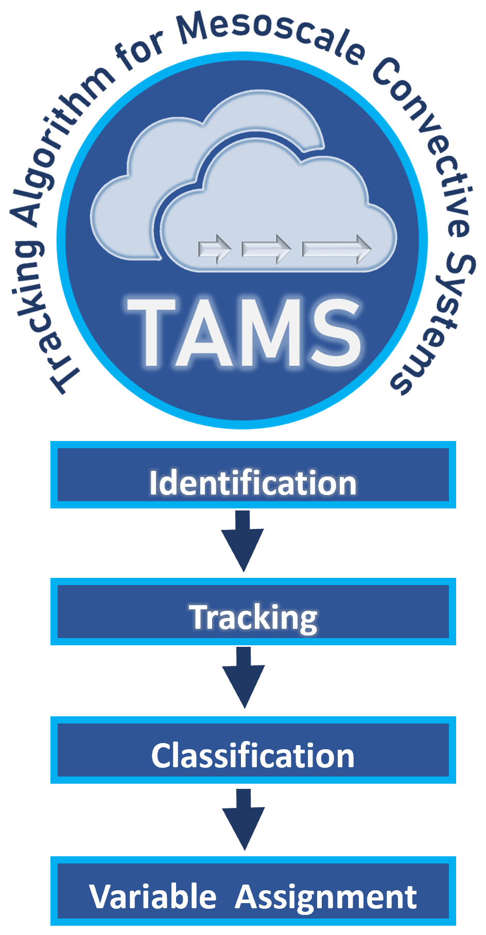
The new version of TAMS (hereon TAMS) is an open-source MCS tracking and classifying Python-based package. A standard workflow using TAMS follows the same main four steps as its predecessor: (1) identify, (2) track, (3) classify, and (4) assign variable(s) (Fig. 1). But the steps can also, to some extent, be run independently. TAMS now includes the capability to assign any desired variable or atmospheric field of choice (not limited to precipitation as in original TAMS) to each mesoscale convective system (MCS) for calculating corresponding statistics of the variable within the cloud area. This new variable assignment functionality, which will be discussed in detail in the following sections, allows TAMS to be customized to identify and track using additional criteria specified by the user rather than solely relying on T_b-dependent criteria. An example of this is the study by Prein et al. (2024) for which TAMS's identification criteria were modified to follow the study's identification criteria.

Figure 1 Schematic of the TAMS logo and the four main algorithm steps.

The TAMS documentation page (https://tams.readthedocs.io/, last access: 7 August 2024) provides a set of instructions for Conda/Mamba or pip installation methods. The package includes a set of visualization, sample datasets, and post-processing tools including functionalities that will be discussed in the following sections. One unique functionality of TAMS is that, like original TAMS, it is grid-independent for tracking, making it a valuable tool for validating simulated MCSs against observed systems. TAMS is additionally grid-independent for assigning variables and supports unstructured-grid input in the identification stage. TAMS provides optional parallelization for (1) CE identification and (2) calculation of statistics of gridded data within MCS and cold-core areas. The TAMS core dependencies are GeoPandas (den Bossche et al., 2023), Matplotlib (Hunter, 2007), NumPy (Harris et al., 2020), pandas (Wes McKinney, 2010; The pandas development team, 2023), scikit-image (van der Walt et al., 2014), Shapely (Gillies et al., 2023), and xarray (Hoyer and Hamman, 2017). The documentation examples are provided as Jupyter Notebooks. The output format is a GeoPandas GeoDataFrame, but this can be transformed into a gridded mask representation, as done for the Prein et al. (2024) tracker intercomparison project (code available in the TAMS GitHub repository). Next, each step of the algorithm will be discussed in detail.

2.1 Identification

The default TAMS identification step follows the approach of the first version using contours of T_b or cloud-top temperature (CTT) data (if using model data) to identify cloud regions (i.e., CEs) of 235 K areas containing embedded 219 K area(s) ≥4000 km². The field used must have associated latitude and longitude coordinate variables. Extremely small 219 K areas (≤10 km²) are discarded, as are 235 K areas that do not meet the 4000 km² threshold. These contour definitions are converted to Shapely polygons, with the convex hull operation applied in order to smooth out the shapes and reduce the number of points required to represent them (to reduce memory requirements and speed up computations). The tams.identify function returns a GeoDataFrame of these shapes. This is the first step of the TAMS workflow, and it can also be run within the tams.run function, which runs all the steps of the workflow with one command (note that if using tams.run, the input xarray DataArray should have both cloud-top temperature and precipitation rate variables). The user is able to modify the identification criteria through the use of the variable-assigning functionality as was done for Prein et al. (2024). This functionality will be described in the next sections. The user does not need to provide time step and grid spacing information to TAMS, but they should be aware of it when considering the overlap threshold and the addition of cloud projection for the tracking step discussed in the next section.

Other parameters in this identification step include enabling parallelization (for input data with a time dimension), the CTT threshold for the cloud boundary, and an additional CTT threshold used to identify the deep convective areas and embedded cold cores. Figure 2 is a visual example using the Meteosat Second Generation (MSG) geostationary satellite (Schmetz et al., 2002), specifically the 10.8 µm spectral band of the Spinning Enhanced Visible and Infrared Imager (SEVIRI) data on 16 September 2022. MCSs coupled to an AEW that were active during research flight 7 of field campaign CPEX-CV (https://espo.nasa.gov/cpex-cv/content/CPEX-CV, last access: 31 October 2023) were identified. The red crosses show the track of the AEW up to that time using the AEW tracker by Lawton et al. (2022). The TAMS package includes sample MSG satellite data that can be loaded using API functions as either the satellite IR radiance (channel 9) or derived T_b. The user can compute the T_b by using an API function that takes MSG SEVIRI IR satellite radiance and channel number as input.

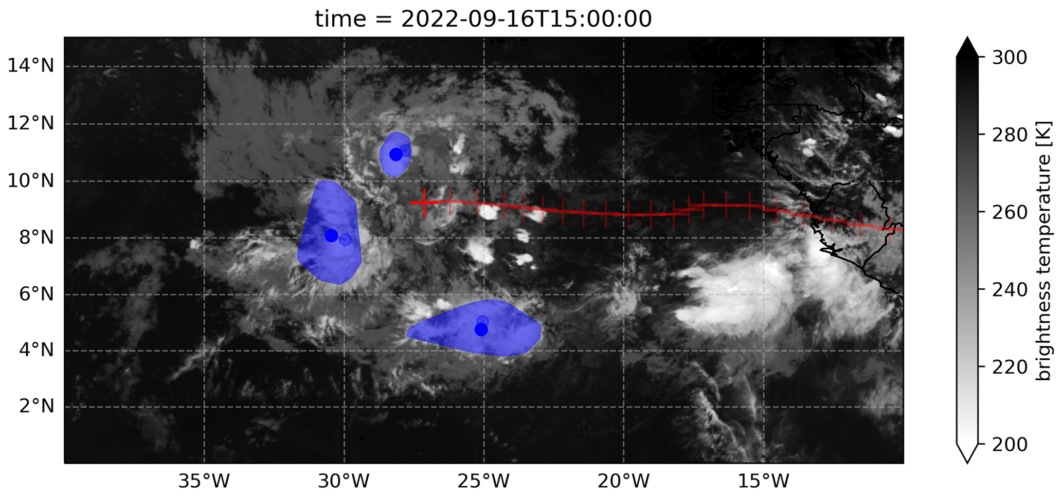
Figure 2 Identified MCSs using MSG data during research flight 7 of the CPEX-CV field campaign. CEs (convex-hull, warm-core 235 K areas) are in blue and IR shaded. Blue dots represent the geographical centroid position. Red crosses are the track of the AEW. Time is in UTC.

Grid-independent identification

TAMS includes sample data taken from a 15 km global-mesh Model for Prediction Across Scales (MPAS) simulation from 8 September 2006 at 12:00 UTC to 13 September 2006 at 18:00 UTC initialized with the Integrated Forecast System (IFS) (Núñez Ocasio and Rios-Berrios, 2023, 2022). This includes native unstructured-grid model output and output regridded to a 0.25° lat–long grid using a first-order conservative method (Jones, 1999) via Climate Data Operators (CDO; https://code.mpimet.mpg.de/projects/cdo, last access: 10 June 2024). To keep file sizes down, the versions included in TAMS are spatial subsets of the original model outputs and include only selected variables. The sample datasets can be automatically downloaded then loaded as xarray objects using API functions.

TAMS is able to identify CEs in both MPAS datasets by contouring the cloud-top temperature (235 K by default). For unstructured-grid data, this currently uses Matplotlib's tricontourf function. In this case, by default, the Delaunay triangulation of the lat–long coordinates is used. Note that this is only an approximation of the true MPAS grid, which is mostly made up of hexagons, but we expect this effect to be insignificant for our high-resolution example. MPAS grids can be decomposed into triangles (e.g., six per hexagon) and the resulting triangulation can be used instead if desired (https://mpas-dev.github.io/MPAS-Tools/stable/visualization.html#mpas-mesh-to-triangles, last access: 7 August 2024) for a faithful representation but with increased contouring compute time. We refer to the identification as grid-independent because we can support unstructured-grid data in addition to structured-grid data with 1-D or 2-D lat–long coordinates.

Figure 3 shows a comparison of MPAS unstructured-grid identified CEs compared to those identified from the MPAS regridded data. The native output is the most faithful to the true model state. Regridding is often done from a higher to a lower spatial resolution, and, depending on the techniques used, CEs may become connected. For example, the CE near 5° N, 105° E in Fig. 3b is separate from the larger CE in the identification using the native MPAS data but not in that using the regridded data.

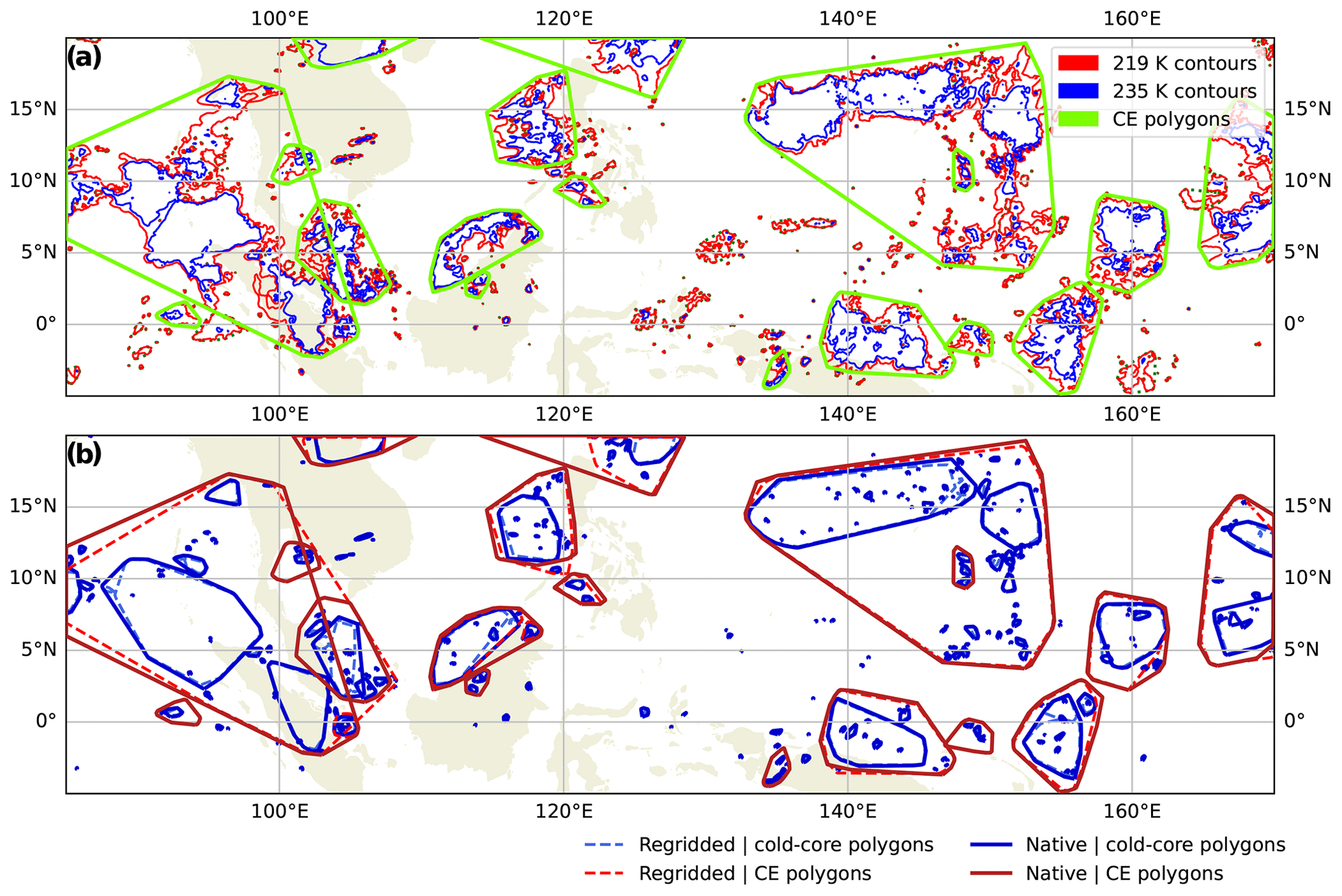
Figure 3 CEs identified on 8 September 2006 at 22:00 UTC (10 h in) for the sample MPAS datasets. (a) Contours of the native MPAS output and associated CE polygons. (b) CEs derived from native (solid lines) MPAS output and regridded (dashed lines) MPAS output.

2.2 Tracking

By default, the track of an MCS is obtained by linking CEs at the current time to CEs at the previous time (backward linking) based on maximum CE polygon overlap. Since the polygons are defined by a set of coordinates (not, e.g., by integer masks on a grid), the tracking can be considered grid-independent. A CE at time t_i has one “parent” at t_i−1, but multiple CEs can have the same parent (e.g., splitting). Optionally, you can choose to have only the largest CE continue a given track as done in Evans and Shemo (1996). Forward linking is also available, and other linking methods are in development.

Overlap thresholds are based on normalized area (0–1), so it is important to consider which area to use when normalizing the overlap area. Núñez Ocasio et al. (2020a) used the minimum area between the two CEs being compared. In this version of TAMS, by default, the area of the CE at the current time when linking is used, but TAMS provides other options: the minimum CE area, maximum CE area, the average, the current CE, or the CE at the other time. As in the first version, there is a setting to project the CE in the x direction before computing overlap, which proves useful when MCSs are propagating in an environment with prevalent zonal background flow, especially when hourly or higher-time-resolution data are not available (Núñez Ocasio et al., 2020a; Feng et al., 2023). The user could estimate what value to use based on a climatology of wind data, but we leave it to the user's discretion to decide on the specific value to choose. Accounting for background flow by projecting the CE before calculating overlap ensures that MCSs that move fast are being tracked. For example, over Africa, the African easterly jet accounts for a large part of the MCS propagation speed. Thus, depending on the resolution being used the user may want to add a projection of −10 m s⁻¹ (Núñez Ocasio et al., 2020a). The track of an MCS is then defined as the record of all CEs linked. It is important to note that, for a given MCS, there may be more than one CE at a given time. To define a single pointwise track in this case, we use the centroid of the combined “multi-polygon” at each time.

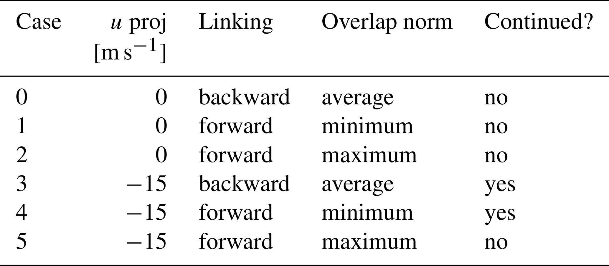
Figure 4 shows MCSs identified and tracked through time (darker shades represent later times) from the sample MSG satellite data using a TAMS API function to plot the tracks. How different setting combinations can be used to link and subsequently alter the track of an MCS is shown in Table 1 for the MCS in the red box in Fig. 4. In order to capture the full track of an MCS that evolved from a larger area to a smaller area as in the example, projection and overlap normalization settings should be carefully selected. Only the two cases with u projection −15 m s⁻¹ and average or minimum overlap normalization continue this track (cases 3 and 4 in Table 1).

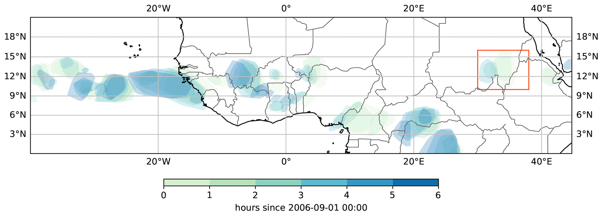
Figure 4 MCS tracks in time (darker shades represent later times) from sample MSG satellite data.

Table 1 Example using different tracking options for an observed MCS case.

A variable that can be analyzed strictly based on the information from the CE and MCS shapes is the area of the systems. Figure 5 shows how the area of simulated MCSs in MPAS is sensitive to threshold temperature selection for identification and to projection speed for tracking. The area is more sensitivity to temperature tuning than projection speed, since there is little noticeable change between the distributions within a certain column. For example, the most likely area range is around 10⁵ km² (consistent with Feng et al., 2023, their Table 1) for all cases in the first column. However, higher projection speed results in a larger number of MCSs in all temperate threshold cases, suggesting that less linking is occurring. Warmer temperature thresholds compared to the defaults (rightmost column) lead to increased system counts and a smoother distribution covering a broader area range. A warmer threshold leads to mergers in the contouring but also provides more new shapes (in this case the latter wins out). On the other hand, much cooler temperature thresholds (left column) pick up about half as many systems, with a distribution that favors larger areas. In this case, the cold-core area criterion is more restrictive.

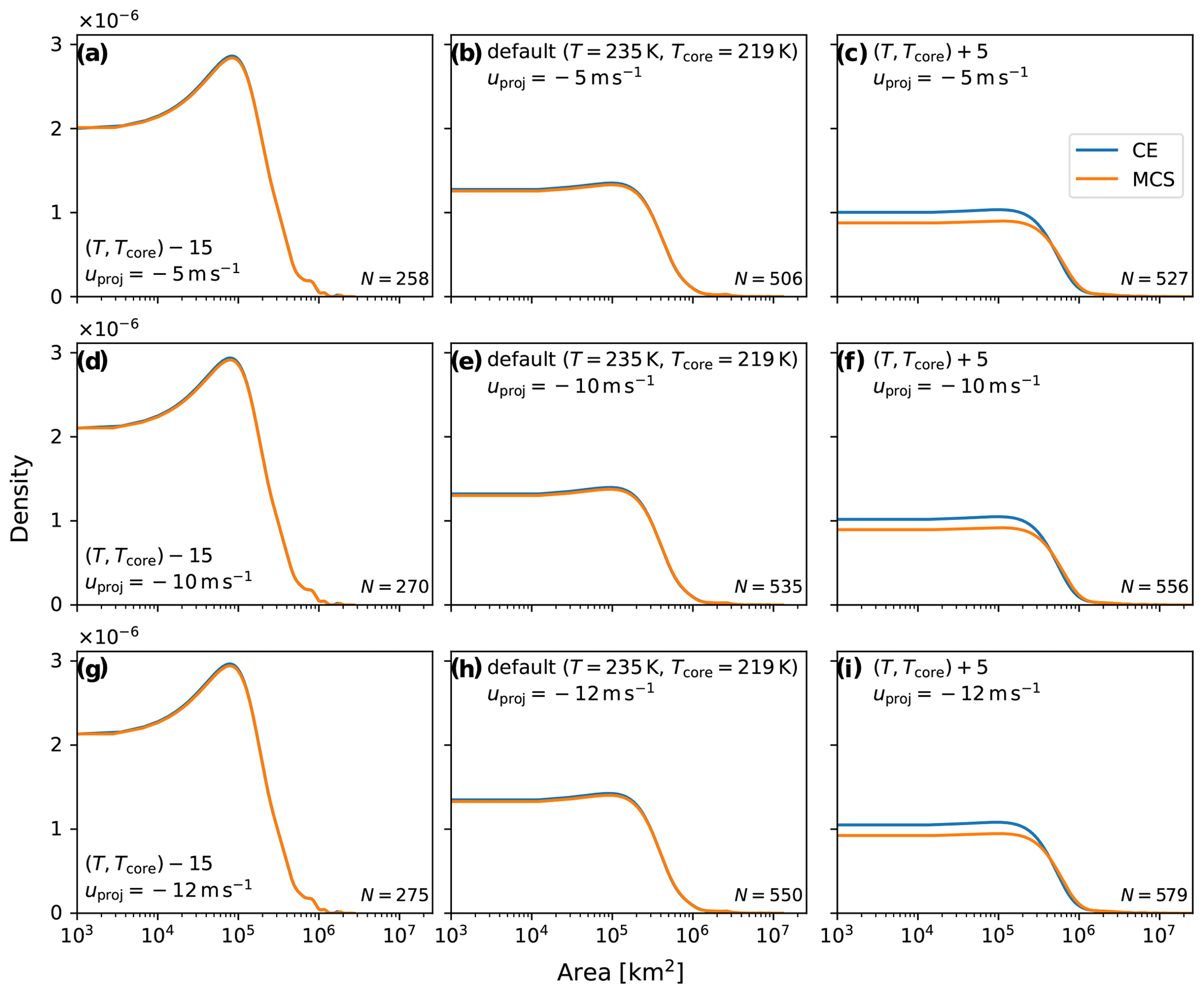
Figure 5 Maximum area kernel density estimates (KDEs) for simulated MCSs from MPAS sample data interpolated to a latitude–longitude grid. Rows represent results using the same projection speed for tracking, while columns represent different temperature thresholds for identification. The data are for the period of 8 September 2006 at 12:00 UTC to 13 September 2006 at 18:00 UTC.

Another way in which the area of MCSs can be analyzed is by comparing it with other MCS characteristics such as duration. Figure 6 shows duration versus area 2-D kernel density estimates (KDEs) for simulated MCSs from MPAS sample data. In this example we see that the systems with the longest duration are not necessarily the largest. Here, except for some outliers, the systems with the longest duration are of low–moderate area, while the largest systems are of low–moderate duration. Moreover, there are different relationships between area and duration between different core thresholds (e.g., the slope is steeper for the colder cases).

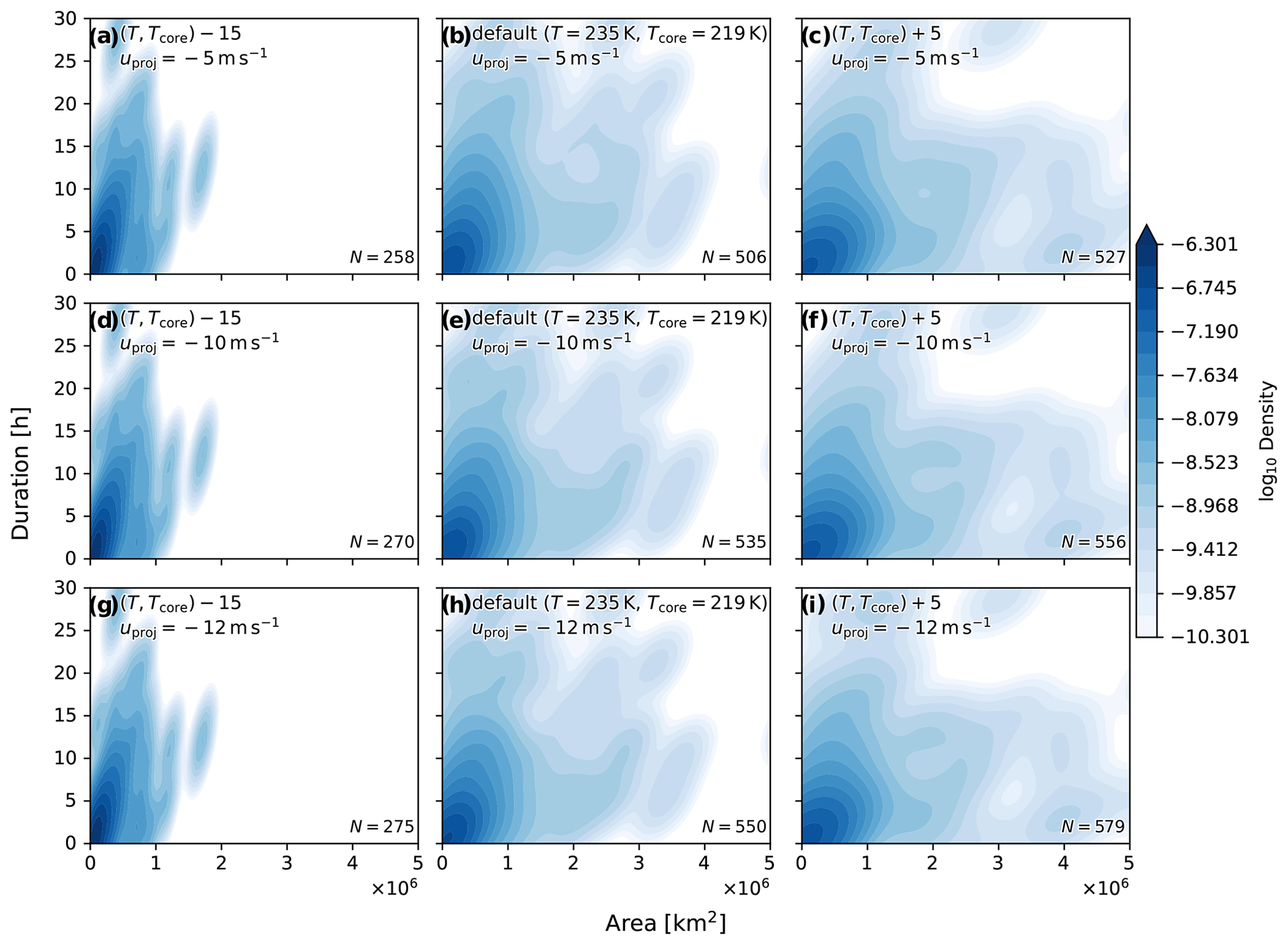
Figure 6 Duration versus maximum area 2-D kernel density estimates (KDEs) for simulated MCSs from MPAS sample data interpolated to a latitude–longitude grid. Rows represent results using the same projection speed for tracking, while columns represent different temperature thresholds for identification. The data are for the period of 8 September 2006 at 12:00 UTC to 13 September 2006 at 18:00 UTC.

2.3 Classification

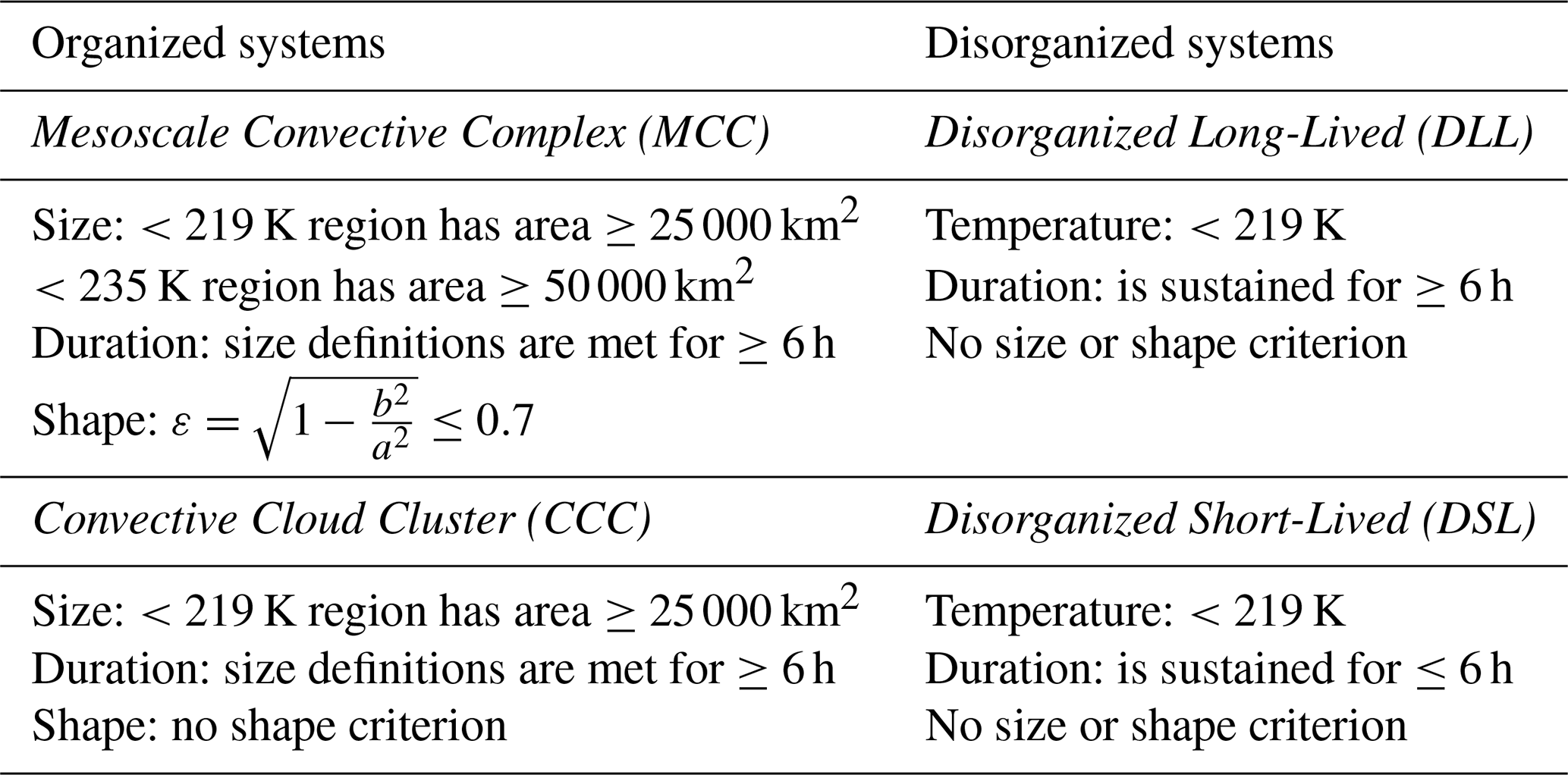
The TAMS software allows the user to classify the entire lifetime of an MCS into one class based on the area, shape, and time criteria described in Table 2. There are four main classes defined in TAMS within two main groups: organized and disorganized systems. The four specific classes are Mesoscale Convective Complexes (MCCs), Convective Cloud Clusters (CCCs), Disorganized Long-Lived (DLL), and Disorganized Short-Lived (DSL). These criteria mostly follow those of the first version in Núñez Ocasio et al. (2020a) with the distinction that DSLs are classified as anything with a duration shorter than 6 h (rather than 3 h or less). Note that these criteria need not be met for consecutive times but for at least 6 h within the lifetime of the system. Recall that all TAMS CEs meet the cold-core criterion.

Table 2 Criteria to categorize the four classes of MCSs.

In order for each MCS to be classified, the user can input the GeoDataFrame obtained from running tams.track into the tams.classify function. The result will be a GeoDataFrame with an additional categorical MCS class column added to the input frame. This GeoDataFrame retains information associated with each CE, and it allows for analyzing the number of CEs versus the number of MCSs by category, as shown in Fig. 7.

Over western Africa during the Fig. 7 example period, the majority of the convection is classified as a DSL. This prevalence of DSLs is notable, as a significant portion of the convection in this region belongs to this category (Fig. 7a and b). Disorganized convective systems are known to be the most frequent type of convective system in the tropics (Rossow et al., 2013; Tan et al., 2013; Semunegus et al., 2017; Núñez Ocasio et al., 2020a). Furthermore, the number of organized MCSs (i.e., MCCs and CCCs) is greatly influenced by the ITCZ, West African monsoon, and AEWs, particularly during the northern summer months (Berry and Thorncroft, 2005; Núñez Ocasio et al., 2020b, 2021; Núñez Ocasio and Rios-Berrios, 2023).

As expected, the number of CEs is much greater than the count of MCSs. (An MCS only gets counted once for its lifetime, while CE counts include counts at each time in the period.) Organized systems (MCCs and CCCs) were less common, with their count below 100. Note that MCCs are defined following Maddox (1980), who defined an MCC as a distinct intense organized and circular convective system (thus the eccentricity criterion). CCCs, which include squall-line-type convection (and thus those that are too elliptically shaped or elongated to be MCCs), were the second-most prominent category during this time. The number of DSL MCSs is comparable to the number of DSL CEs due to the shorter MCS durations. Duration box plots, as shown in Fig. 7c, can help the user discern differences in the duration of the systems across categories. Although CCCs and MCSs share the same time criterion, it is evident that over September 2022, MCCs, based on the median, lasted longer than CCCs.

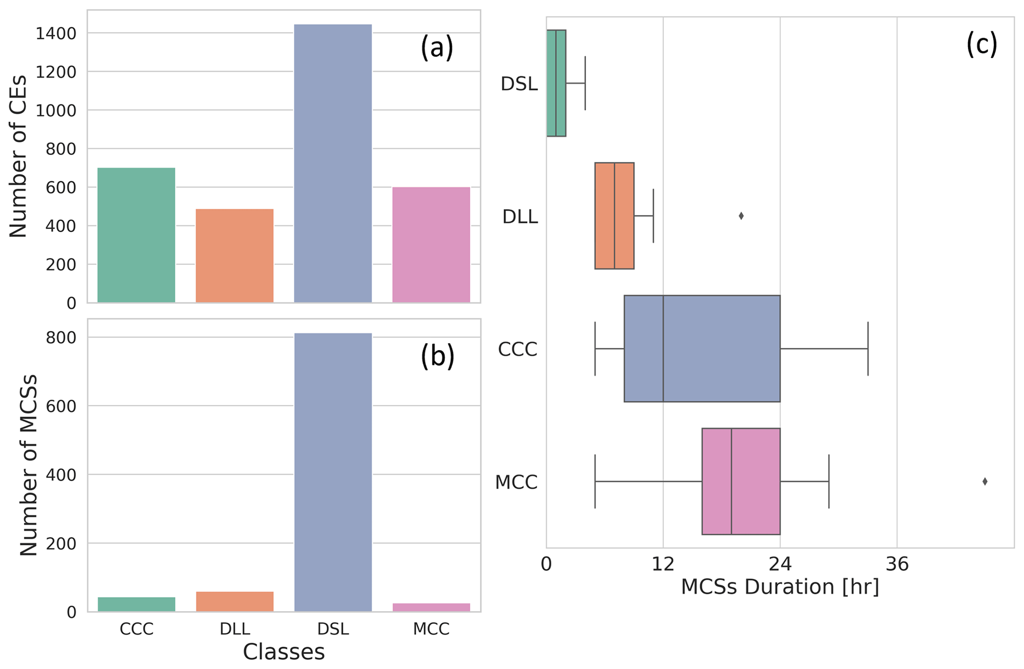
Figure 7 Example statistics for the observed number of CEs (a) and MCSs (b), as well as the duration of MCSs by category (c) during 4 through 30 September 2022, the period of the CPEX-CV field campaign, over a western African domain.

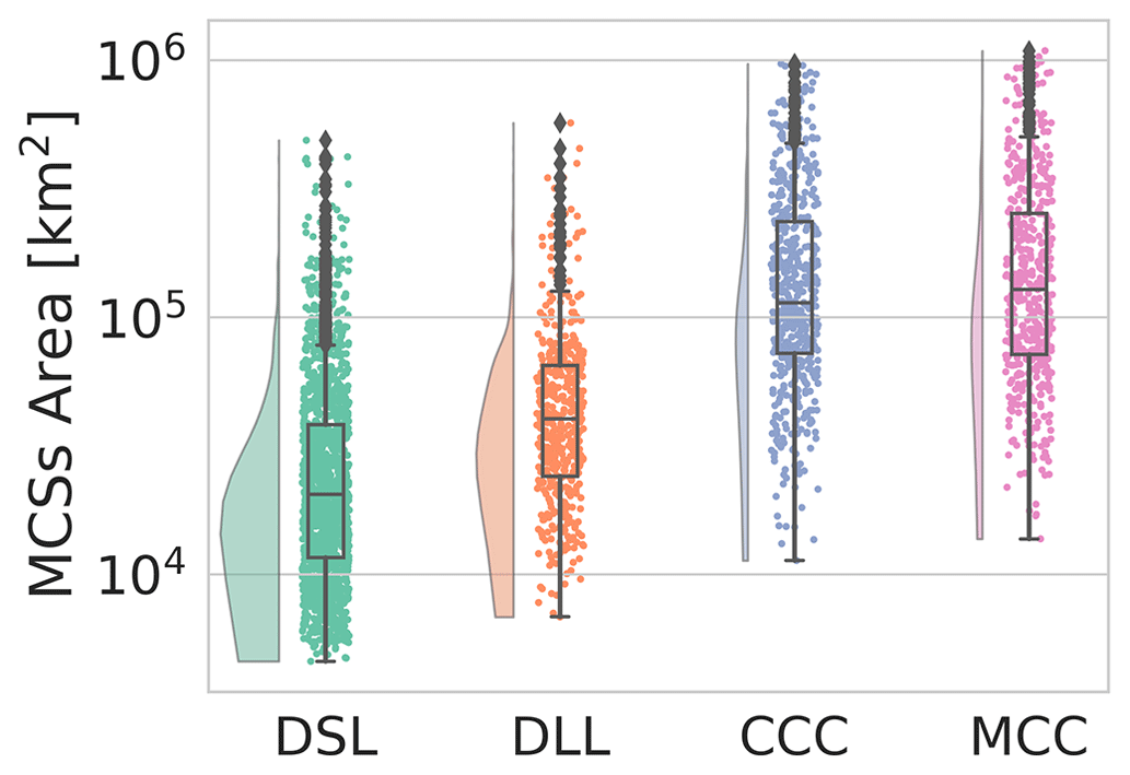
Figure 8 displays MCS area distributions from the CPEX-CV field campaign, categorized by their respective types. During this period, disorganized systems (DSLs and DLLs) were generally smaller than organized systems (MCCs and CCCs), with MCCs, as expected, having the largest median area.

Figure 8 Rain-cloud plots of MCS area (note the log scale) by category for the same period and domain as in Fig. 7.

2.4 Variable assignment

Another unique functionality of TAMS, in addition to identifying and tracking systems using CE polygons and being grid-independent, is its ability to assign any variable of choice to CE or MCS shapes and compute related statistics (e.g., mean and standard deviation) on the data within using a TAMS API function. The statistics are computed over the entire MCS but users can also apply the tooling to compute statistics over the CEs. If tams.run is used instead of running each step separately, the statistics will also include the mean and standard deviation of the cold-core temperature and mean precipitation rates. This allows users to assess the evolution, characteristics, and nature of the systems under study using different atmospheric variables. This function is not limited to a specific data type, spatial resolution, or a specific grid, as demonstrated in the previous sections. Having the same temporal resolution or at least data that include the same times allows the user to match variables to each MCS across various datasets. The geospatial selection process treats the input data as points; only latitude and longitude coordinates are needed, and these need not be the same as those of the data used for CE identification. A visual example of how the variable assignment works is shown in Fig. 9, which demonstrates that the geospatial selection also works for unstructured-grid data.

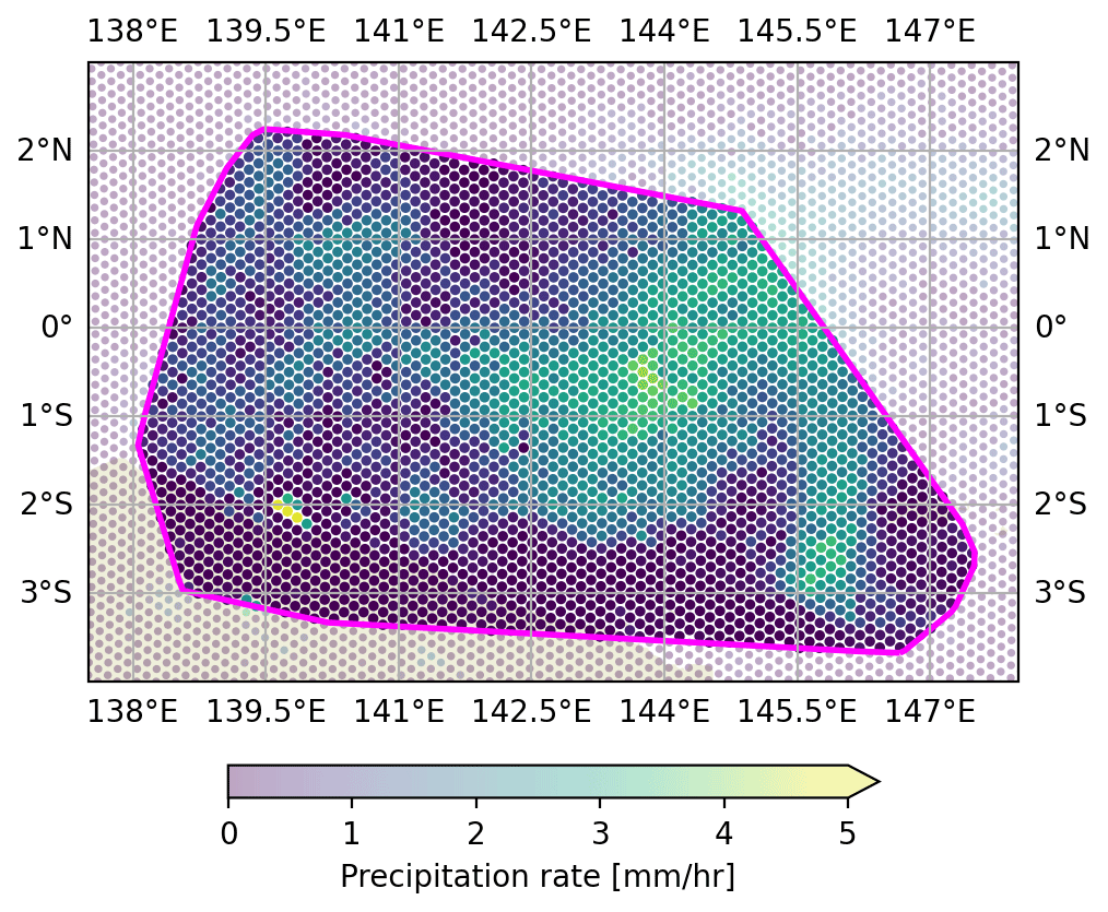
Figure 9 Visualization of the variable assignment of precipitation within a CE selected from Fig. 3b.

One common example is assigning precipitation to each MCS from satellite-derived products like IMERG, as shown in Fig. 10a for the example period of observed MCSs. The statistics include each of the time steps of the MCSs (the CEs of an MCS are combined before creating the plot). DSLs, which had the greatest number of counts, were the rainiest type of MCSs. However, the precipitation rate median of CCCs and MCCs was slightly above that of DSLs at about 3 mm h⁻¹.

Through this function, the user can also extract the minimum T_b as a diagnostic for convection intensity. In Fig. 10b, the most intense and coldest cloud tops were observed in MCCs during the example period. If the user or researcher is analyzing model data that provide a full array of 2-D and 3-D variables at each grid cell, they are not limited to just cloud-top temperature or precipitation. With this functionality, they can assign many other variables and compute relevant statistics.

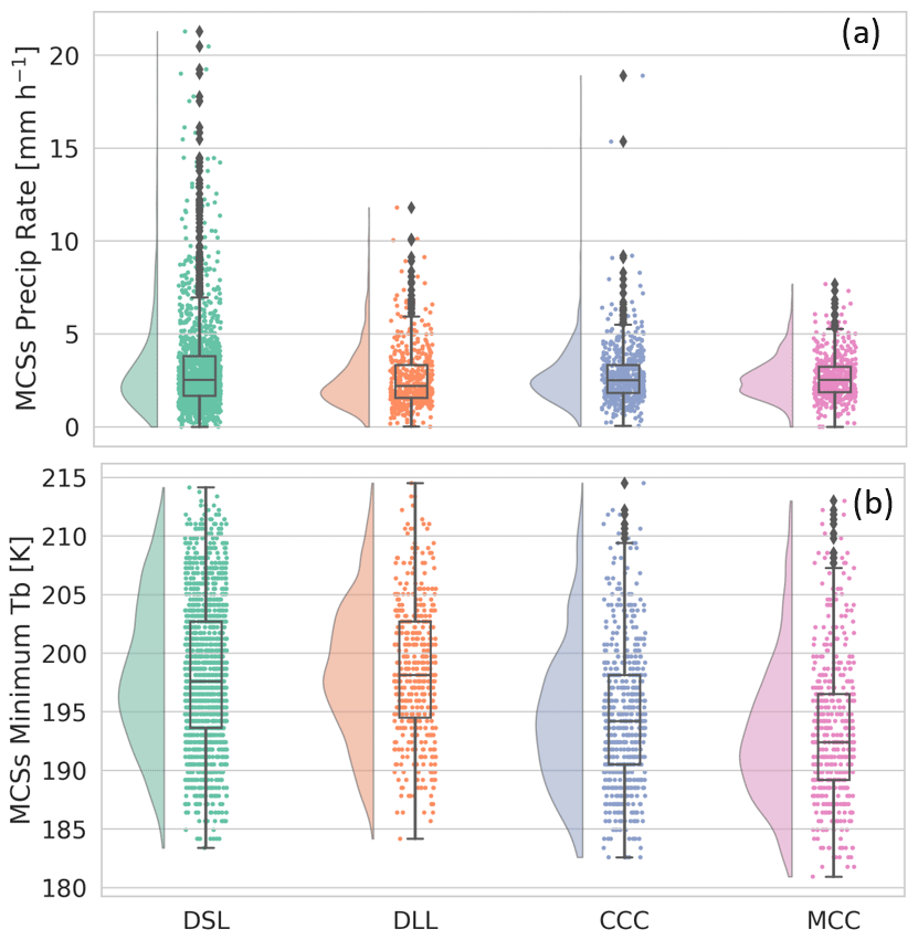
Figure 10 Rain-cloud plots of MCS area-mean rain rates (a) and MCS minimum T_b (b) by category for the same period as in Fig. 7.

As another example, Fig. 11 shows 2-D distributions of simulated precipitation rate versus minimum T_b across different setting options. For this particular subset of data, there is no distinct relationship between minimum T_b and average precipitation rates. Most of the differences across the setting options are due to sensitivity to the change in temperature threshold for identification than to the selected projection speed as discussed in Sect. 2.2. The sample simulated precipitation rate dataset can be loaded with an API function.

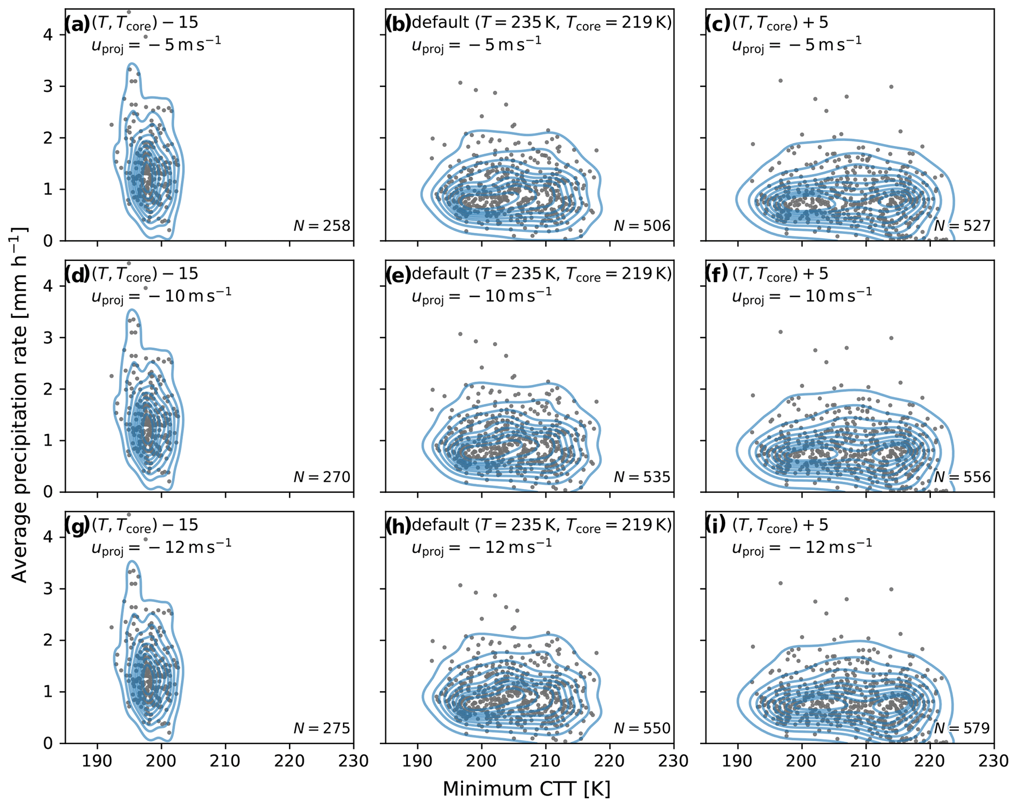
Figure 11 2-D precipitation rate versus minimum T_b kernel density estimates (KDEs) for simulated MCSs from MPAS sample data interpolated to a latitude–longitude grid. Rows represent results using the same projection speeds for tracking, while columns represent different temperature thresholds for identification. The data are for the period of 8 September 2006 at 12:00 UTC to 13 September 2006 at 18:00 UTC, as in Fig. 5.

3 Additional tools and helper functions

3.1 Eccentricity calculation

A quantity that can provide information about the structure of the system is eccentricity (Evans and Shemo, 1996; Núñez Ocasio et al., 2020a). A TAMS API function can be used to calculate the first eccentricity ($\mathit{ϵ}=\sqrt{\mathrm{1}-b^{\mathrm{2}}/a^{\mathrm{2}}}$) of the least-squares best-fit ellipse to the coordinates of the polygon's exterior. If the first eccentricity is ≤0.7, the system is considered more circular (a circle has ϵ=0). This is used in the default MCS classification.

Figure 12 displays the evolution of eccentricity over time, along with other relevant variables, for an observed MCS identified and tracked during research flight 8 of the CPEX-CV field campaign on 20 September 2022. This system persisted for 4 h, and TAMS classified it as a DLL. Initially, the system exhibited a more elongated shape, reaching its precipitation rate peak 1 h after initiation. As time progressed, the system gradually expanded and became more circular. By the time of dissipation, it had evolved into a large and nearly circular system, indicative of a dissipating anvil.

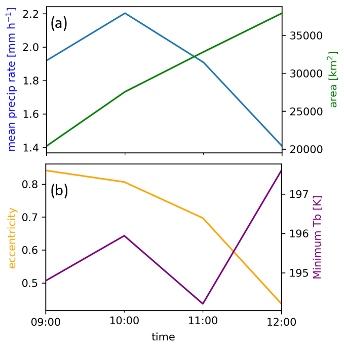
Figure 12 Time series of the observed MCS during research flight 8 of the CPEX-CV field campaign fr precipitation rate (blue line) and area (green line) (a), as well as eccentricity (yellow line) and minimum T_b (orange line) (b).

3.2 Estimating cloud-top temperature from simulated OLR

TAMS also includes code to estimate the cloud-top temperature from simulated top-of-the-atmosphere outgoing longwave radiation (OLR) following the Stefan–Boltzmann law. This is used within the function that was used to load simulations nearing near-real-time application for the PRECIP field campaign. The Yang and Slingo (2001) method, which puts observed infrared brightness temperature and that derived from model OLR on a more equal footing, has also been implemented, and others are planned. It is important to note that these methods really give infrared brightness temperature, which is related to but not the same as the cloud-top temperature.

3.3 Post-processing and visualization

Additional examples featuring the sample data and visualizations can be found within the documentation (https://tams.readthedocs.io/, last access: 7 August 2024) like the plotting of spatial maps including the convex hull outlines of CEs as in Fig. 4. Example applications can be found in the example directory of the GitHub repository. Post-processing and code for Figs. 4, 5, 6, and 11 which show the different tracking and identification options, as well as the use of the example dataset loader functions, can be found in the documentation under examples. These examples also show the statistics that can be derived quickly via high-level functions. Similarly, the code for Fig. 3, demonstrating tracking on unstructured-grid data, is published in the documentation.

4 Summary

We have introduced and described TAMS, an open-source MCS tracking and classifying Python-based package available through GitHub that can be used to study both observed and simulated MCSs. In addition to describing each of the core steps of the algorithm – (1) identify, (2) track, (3) classify, and (4) assign variable(s) – we have introduced visualization and post-processing tools within the package to facilitate the analysis of MCSs for users. What distinguishes TAMS from other tracking packages is its specific design for tracking MCSs. However, the identification and tracking components are flexible and could easily be applied to variables other than cloud-top temperature for different tracking situations. The identification of MCSs is grid-independent, and the user can assign any desired variable to compute statistics on it within the MCS area over time. Current settings and helper functions enable various ways to calculate overlap and account for background flow. The user can select the preferred threshold temperature for the larger convective area to be detected and tracked, as well as the threshold for the corresponding cold cores. Options to select the desired linking method (backward or forward, keep largest, etc.) are also available. Through the sample data available, we have shown that TAMS works with satellite and model data, as well as with unstructured-grid native MPAS data.

4.1 Applications

Recently, TAMS was applied as an MCS forecasting tool using MPAS near-real-time forecast in recent PRECIP (http://precip.org/, last access: 12 December 2023) and CPEX-CV (https://ghrc.nsstc.nasa.gov/home/field-campaigns/cpex-cv, last access: 12 December 2023) field campaigns. In addition, TAMS is one of six MCS tracking algorithms participating in a multi-MCS-tracking intercomparison study (Prein et al., 2024), which is part of the NSF NCAR South America Affinity Group (SAAG; Dominguez et al., 2023) (https://ral.ucar.edu/projects/south-america-affinity-group-saag, last access: 12 December 2023) to study MCSs over South America. The specific TAMS SAAG application is located under examples/mosa in the GitHub repository. PyFLEXTRKR, MOAPP, ForTraCC, tobac, and TOOCAN are also involved in this study.

TAMS is being used internationally for MCS detection and tracking. Currently, TAMS is part of a second multi-MCS-tracking intercomparison study that is making use of high-resolution global simulations from DYAMOND (https://www.esiwace.eu/the-project/past-phases/dyamond-initiative, last access: 12 December 2023) to analyze MCSs globally. We hope TAMS can serve the scientific and research community worldwide, facilitating the study of observed and simulated MCSs. We very much welcome contributors to the code.

4.2 Caveats

There are a couple of caveats associated with the software that are worth noting. The use of a convex hull to define CEs introduces some systematic bias towards larger areas. This could potentially lead to an artificial increase in the calculated system's propagation speed relative to the geographical centroid. More generally, however, computing overlap with convex hull shapes allows for a larger likelihood of linking compared to more strict contour shapes. Additionally, for users interested in analyzing a convective system from its very early initiation stages as a convective cell, the TAMS identification criterion of requiring an embedded 219 K core can sometimes inhibit the detection of these early system stages. However, it is important to mention that users have the flexibility to alter the criteria used in the software's settings.

4.3 Development goals

Our development goals encompass the incorporation of additional settings into our system. These new settings include, but are not limited to, the following.

1. Include other methods for computing CTT from T_b.

2. Implement a projection option based on trajectory history.

3. Implement the original TAMS linking method for comparison.

4. Implement a graph-based linking method with pruning for better handling of (and recording of) both merging and splitting.

5. In CE identification, make the application of the convex hull operation optional, and support other shape-simplification options such as a buffer.

6. Combine an AEW tracker (Lawton et al., 2022) with TAMS, as detailed in the study by Núñez Ocasio et al. (2020b).

7. Extract the code for reducing the CE dataframe to the MCS dataframe and the reduction from the MCS dataframe to the MCS stats dataframe so that it can be used in custom workflows outside of tams.run

8. Add more documentation examples, including testing of generated idealized cases.