HSW-V v1.0: localized injections of interactive volcanic aerosols and their climate impacts in a simple general circulation model

A new set of standalone parameterizations is presented for simulating the injection, evolution, and radiative forcing by stratospheric volcanic aerosols against an idealized Held–Suarez–Williamson (HSW) atmospheric background in the Energy Exascale Earth System Model version 2 (E3SMv2). In this model configuration (HSW with enabled volcanism, HSW-V), sulfur dioxide (SO₂) and ash are injected into the atmosphere with a specified profile in the vertical, and they proceed to follow a simple exponential decay. The SO₂ decay is modeled as a perfect conversion to a long-living sulfate aerosol which persists in the stratosphere. All three species are implemented as tracers in the model framework and are transported by the dynamical core's advection algorithm. The aerosols contribute simultaneously to local heating of the stratosphere and cooling of the surface by a simple plane-parallel Beer–Lambert law applied on two zonally symmetric radiation broadbands in the longwave and shortwave ranges. It is shown that the implementation parameters can be tuned to produce realistic temperature anomaly signatures of large volcanic events. In particular, results are shown for an ensemble of runs that mimic the volcanic eruption of Mt. Pinatubo in 1991. The design requires no coupling to microphysical subgrid-scale parameterizations and thus approaches the computational affordability of prescribed aerosol forcing strategies. The idealized simulations contain a single isolated volcanic event against a statistically uniform climate, where no background aerosols or other sources of externally forced variability are present. HSW-V represents a simpler-to-understand tool for the development of climate source-to-impact attribution methods.

1 Introduction

Volcanic eruptions are one of the most dominant natural sources of exogenous forcing on the Earth system. In large volcanic events, the stratosphere can be loaded with extraordinary amounts of sulfur dioxide (SO₂) that gradually oxidize to form long-living sulfate aerosols (Bekki, 1995). In the case of tropical eruptions, the radiative properties of long-living aerosols subsequently lead to global stratospheric and surface-level temperature deviations of up to a few Kelvin from climatological averages, which can persist for years (Kremser et al., 2016; McCormick et al., 1995; Dutton and Christy, 1992). Variations in the stratospheric sulfate content from Earth's volcanic history have thus been one of the strongest drivers of interannual climate variability (Schurer et al., 2013).

Since volcanic eruptions impact the climate, there is a rich history of implementing volcanic forcing parameterizations for coupled Earth system models (ESMs) in the literature. Simpler techniques prescribe radiative aerosol properties directly from an external dataset or analytic forms (DallaSanta et al., 2019; Toohey et al., 2016; Eyring et al., 2013; Gao et al., 2008; Kovilakam et al., 2020). Prescribed forcing approaches might be chosen for their computational affordability, though they are also used to facilitate climate model intercomparisons by standardizing the forcing scheme (Zanchettin et al., 2016; Clyne et al., 2021). More complex approaches prescribe emissions of volcanic SO₂, which are then handed to separate aerosol, chemistry, and advection codes. These codes then explicitly model the aerosol evolution, transport, and radiative properties (Mills et al., 2016, 2017; Brown et al., 2024). Reviews of the wide array of modeling choices for volcanic forcings made by different ESMs are presented in Timmreck (2012) and Marshall et al. (2022).

Prescribed and prognostic methods have also been applied to model other forms of sulfur-based radiative forcing, with significant research recently being devoted to stratospheric aerosol injection (SAI) climate change intervention activities (Crutzen, 2006; Tilmes et al., 2018, 2017; McCusker et al., 2012). One key goal of SAI research is to quantify the causal connections between an observed climate impact and an upstream forcing source, i.e., to attribute the SAI source as the cause of a detected, anomalous atmospheric response. Volcanoes are a natural analog to SAI and thus offer an avenue for developing novel attribution methods of quantifying these causal connections.

The climate impacts that are most societally relevant tend to be spatially localized (e.g., droughts, heat waves, or fires) and located downstream from their associated sources (e.g., volcanoes or other solar radiation modification) by multiple causal connections. Multistep attribution involves a sequence of single-step attribution analyses but is generally not employed, as the single weakest attribution step limits its confidence (Hegerl et al., 2010). Therefore, there is a need for novel multistep attribution techniques in both climate change studies (Burger et al., 2020) and climate intervention studies (National Academies of Sciences and Medicine, 2021; Office of Science and Technology Policy (OSTP), 2023) that overcome these issues to enable attribution of societally relevant impacts.

As the climate community increasingly relies on advanced statistical inference and machine learning approaches to attribute downstream impacts, it is critical to develop test beds which can be widely shared and used to understand the accuracy of the methods' inferences. Although the development of verification datasets for advanced data analytic techniques in the climate community is nascent, there are a few examples. Fulton and Hegerl (2021) generated synthetic climate modes to test the accuracy of distinct pattern extraction techniques and show that the most commonly used principal component analysis technique does not perform well. Mamalakis et al. (2022) worked to develop an “attribution benchmark dataset” for which the ground truth is known to enable evaluation of different explainable artificial intelligence (AI) methods.

Currently, developing data analytic methods for multistep attribution in the context of volcanic forcing is restricted to models that utilize expensive prognostic aerosol treatments. This is because, with prescribed forcing approaches in free-running atmospheric simulations, there is a dynamical inconsistency between the transport patterns and the aerosol distributions. In particular, the forcing dataset does not respond to the atmospheric state. Accordingly, we suggest that a new idealized representation of prognostic volcanic forcing within a highly simplified atmospheric environment would be a useful test bed for the development of novel multistep attribution methods (i.e., constructing relationships between stratospheric aerosol forcing and atmospheric temperature perturbations).

Here we outline a simulation strategy which enables an affordable prognostic aerosol implementation for idealized climate model configurations. Our design seeks to maintain a realistic spatiotemporal signature of the atmospheric impacts while minimizing the terms contributing to temperature and wind tendencies as much as possible. The former is achieved by including a localized injection and subsequent transport of aerosols by a tracer advection scheme. The latter is achieved by coupling the aerosol concentrations directly to the temperature field. While traditional approaches often require the inclusion of an auxiliary radiative transfer code for this second step, our implementation is standalone.

Our approach sacrifices realism by design. The goal is not to simulate an accurate post-eruption climate of a particular historical volcanic event but rather to produce a plausible realization of a generic volcanic eruption, simulated with a minimal forcing set. This configuration will not offer a deterministic answer to the attribution problem, as the internal variability of the simulated atmosphere implies that there is no single solution to the spatiotemporal evolution of the affordable prognostic aerosol. Nevertheless, it does represent key process characteristics between a source and downstream impact and can provide large datasets without the typical computational burden of climate simulations, thereby supporting the development and testing of novel data analyses and attribution techniques.

Our model isolates a single volcanic event from any other external source of forcing or variability and allows the flexibility to be embedded in a simplified atmospheric environment. Though the implementation is generic, here we present a particular tuning of the parameterizations for an eruption similar in character to the 1991 eruption of Mt. Pinatubo and the subsequently observed impacts (Karpechko et al., 2010; Robock, 2000; McCormick et al., 1995; Hansen et al., 1992). The atmospheric model is an idealized so-called Held–Suarez–Williamson (HSW; Williamson et al., 1998) configuration of the Energy Exascale Earth System Model version 2 (E3SMv2; Golaz et al., 2022). The HSW configuration on a flat Earth replaces E3SMv2's physical parameterization package with a temperature relaxation towards a prescribed, hemispherically symmetric equilibrium temperature and Rayleigh friction near the surface. These two forcing mechanisms mimic radiative effects and the boundary-layer turbulence, respectively. There are no background aerosols, no moisture, and no long-term climate trends. The implementation of the injection, aerosol dissipation, and forcing can be tuned to yield sensible atmospheric impacts for almost any model configuration with qualitatively realistic circulation patterns, even in the absence of a standard physical parameterization suite. We call this extension to the HSW model with enabled volcanism HSW-V.

The paper is structured as follows. The simplified climate model configuration of E3SMv2 is described in Sect. 2. Section 3 introduces the idealized volcanic injection, sulfate formation, and radiative forcing parameterizations. This is followed by a discussion of the ensemble design, simulation results, and computational expense in Sect. 4. Section 5 summarizes the findings and provides an overview of their utility for the modeling community. Appendix A describes custom modifications that were needed for our chosen simplified climate implementation with E3SMv2. In addition, Appendix C provides recommendations for the tuning of the suggested aerosol parameterizations.

2 Climate model configuration

When choosing the base model configuration, the goal was to provide an environment in which the volcanic forcing can be nearly isolated. In addition, we aimed to keep the number of physical subgrid-scale forcing mechanisms small. These simplifications are achieved by running a climate model in atmosphere-only mode and replacing the standard suite of physical parameterizations with simple forcing functions for the temperature and horizontal winds.

Section 2.1 introduces the E3SMv2 climate model, which serves as the foundation for our developments. E3SMv2's chosen HSW configuration is a modified implementation of the idealized scheme originally described by Held and Suarez (1994) (hereafter HS94), involving a damping of low-level winds and a relaxation of the temperature field to a specified zonally symmetric reference profile described in Sect. 2.2. The main difference between the Held and Suarez (1994) and HSW forcing is the presence of a more realistic relaxation temperature profile above 100 hPa which generates stratospheric polar jets in the HSW variant. Section 2.3 describes a simple extension for idealized physics packages which provides global, zonally symmetric longwave and shortwave radiation profiles.

2.1 The E3SMv2 climate model

E3SMv2 is a state-of-the-art climate model that consists of various coupled components for the atmosphere, ocean, land, sea ice, and land ice (Golaz et al., 2022). The dynamical core of the E3SM Atmosphere Model version 2 (EAMv2) uses a spectral-element (SE) solver on a quasi-uniform cubed-sphere grid for a shallow, hydrostatic atmosphere (Taylor et al., 2020) and a semi-Lagrangian tracer transport scheme (Bradley et al., 2022), which ensures local mass conservation and shape preservation. Specifically, the experiments presented here use the ∼ 2° “ne16pg2” grid, where each cubed-sphere element features a 2×2 grid of physics columns. The grid for the physical parameterizations is thus coarser than the associated dynamics grid (Hannah et al., 2021; Herrington et al., 2019). The vertical grid consists of 72 vertical levels with a model top near 0.1 hPa, or approximately 60 km.

We use a highly simplified, dry configuration of EAMv2 with no topography, no moisture, and no coupling to other components. The physical parameterization suite is replaced with a set of idealized forcing functions described in Sect. 2.2. Internally, this configuration is labeled the “FIDEAL” component set – an inheritance of E3SMv2 from its original fork of the Community Earth System Model (CESM, Danabasoglu et al., 2020). As a part of our work, the FIDEAL component set needed to be revived and is not functional in the official release of E3SMv2.

We note that the ne16pg2 grid is coarser than the default E3SMv2 ∼ 1° “ne30pg2” grid. We have not tested activating our implementation on such a higher-resolution grid, which will require retuning of the model parameters. Recommendations for performing the tuning of the volcanic forcing are given in Appendix C.

2.2 Idealized climate forcing

The Held and Suarez (1994) forcing was originally proposed as a benchmark for the intercomparison of statistically steady states produced by the dry dynamical cores of atmospheric general circulation models (AGCMs) without topography. The forcing includes Rayleigh damping of low-level winds to represent friction in the boundary layer and a Newtonian temperature relaxation toward an analytical “radiative equilibrium” temperature T_eq(ϕ,p) given by

$$\begin{array}{}\text{(1)}& {\displaystyle \frac{\partial T}{\partial t}}=\mathrm{\dots }-k_T(\mathit{\varphi },p)\left[T-T_{\text{eq}}(\mathit{\varphi },p)\right].\end{array}$$

Here, T is the temperature, t stands for the time, ϕ represents the latitude, p symbolizes the pressure, and k_T(ϕ,p) is the relaxation rate. T_eq has no time dependence and therefore does not include any diurnal or seasonal cycles. The temperature variability on any timescale is purely driven by the internal dynamics arising from nudging towards the equilibrium. The form of the equilibrium temperature is designed to mimic the net effects of radiation, convection, and other subgrid-scale processes. Williamson et al. (1998) (hereafter W98) later noted that since the Held and Suarez (1994) benchmark deliberately maintains a “passive” stratosphere, supporting none of the typical stratospheric structures such as the polar jets, it would not be applicable to their dynamical core intercomparison studies of tropopause formation. To remedy this deficiency, they provided a modification of the original Held and Suarez (1994) equilibrium temperature, which included realistic lower-stratospheric lapse rates in the tropics and the polar regions. Such a HSW configuration was, e.g., also used in Yao and Jablonowski (2016), who explored sudden stratospheric warmings (SSWs) in the idealized environment.

We use the HSW forcing in our simulations and omit all other physical parameterizations. This setup provides an atmosphere that is characterized by realistic dynamical motions and a quasi-realistic idealized climatology while maintaining a highly simplified inventory of diabatic subgrid forcings. In implementing the HSW configuration in E3SMv2, a few notable modifications were made. First, the lapse rate of the equilibrium temperature T_eq was set to zero above 2 hPa to maintain realistic upper-stratospheric temperatures. Next, in addition to the Held and Suarez (1994) treatment of surface friction, we include a second Rayleigh damping mechanism near the model top as a “sponge layer” to calm the polar jet winds and absorbing spurious wave reflections, as described in Jablonowski and Williamson (2011). The specifics of these HSW modifications are provided in Appendix A.

Figure 1 shows the equilibrium temperature in the latitude–pressure plane, the vertical profile of the wind-damping strength, and the resulting 10-year average zonal-mean temperature and zonal-wind fields following a 5-year spinup period using these idealized forcings in E3SMv2. The resulting stratospheric temperature and wind structures are quasi-realistic, reaching maximum tropical temperatures of about 240 K at the 50–60 km height levels which correspond to the region between 1 and 0.1 hPa. However, these temperatures are slightly cooler than the observed values near 50 km (1 hPa), which are about 260 K, as documented in Fleming et al. (1990). Temperature minima are seen near the tropical tropopause as well as the polar middle stratosphere. Sharp vertical temperature gradients are seen near the polar upper stratosphere, leading to temperatures in excess of 270 K.

In the zonal wind, we see the formation of tropospheric midlatitude westerly jets with maximum wind speeds of ∼ 30 m s⁻¹ and strong stratospheric polar jets in excess of 60 m s⁻¹. As there are no seasonal variations present, each hemisphere eternally varies about this winter-like steady state, which is qualitatively representative of observations (Fleming et al., 1990). At the same time, the global circulation, and thus mass transport, is characterized by symmetric thermally direct circulations (Hadley cells) in the troposphere and symmetric residual streamfunction cells in the stratosphere, consistent with equinox states in nature (see the discussions in Sect. 4.2 and Appendix B).

In the tropical stratosphere, easterlies with speeds up to −30 m s⁻¹ dominate. Note that, while the tropical stratospheric winds will vary about this average, the HSW atmosphere does not include any kind of regular quasi-biennial oscillation (QBO) analog. Yao and Jablonowski (2016) showed that whether or not a QBO spontaneously develops in an HSW configuration will largely depend on the dynamical core in use. For an SE dynamical core, they observed that wave forcing was never strong enough to cause a reversal of the tropical stratospheric winds. The same conclusion appears to hold for our configuration of E3SMv2. Despite this, the QBO may be a desirable target for future studies employing this model configuration, as it has been shown that the QBO phase is a significant modulator of the volcanic climate response (Thomas et al., 2009). We do not consider this issue further in the present work but note that it could be possible to prescribe a QBO by nudging the horizontal winds toward a specified reference state (as has been done for, e.g., the Whole Atmosphere Community Climate Model (WACCM) by Matthes et al., 2010).

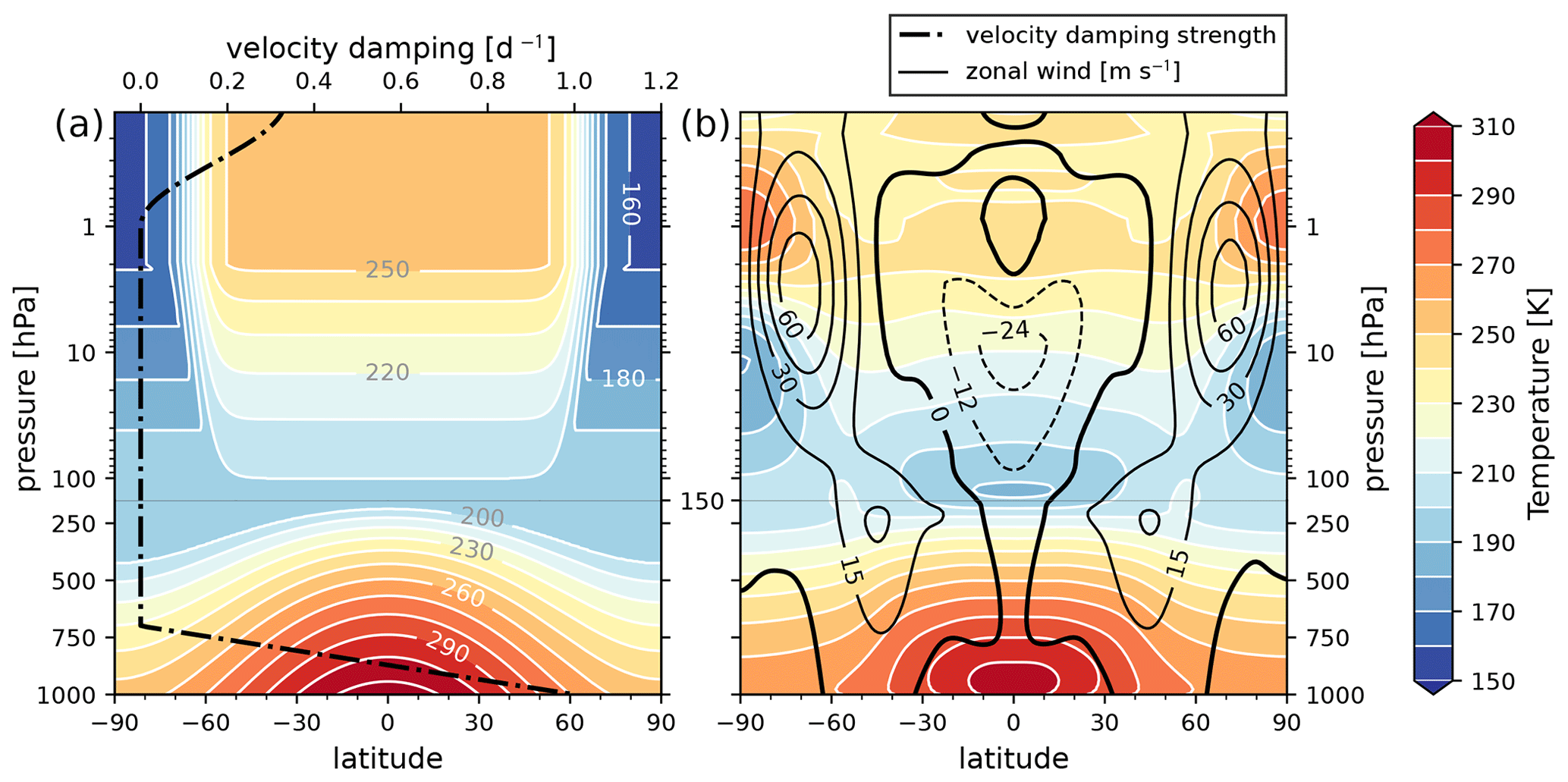
Figure 1 (a) The modified HSW equilibrium temperature in the latitude–pressure plane. Contours are drawn every 10 K. Overlaid as a thick dashed black line is the vertical profile of the velocity damping coefficient for both the sponge layer and the surface, with its values on the top horizontal axis (see Appendix A for details). (b) The 10-year average zonal-mean temperature and zonal-wind distributions in an E3SMv2 run with temperature relaxation toward the reference temperature of panel (a), after a 5-year spinup period. Temperature contours are drawn every 10 K, with positive (negative) wind contours every 15 m s⁻¹ (12 m s⁻¹). Negative contours are dashed, and the zero line is shown in bold. For all the variables shown, the vertical (pressure) axis is logarithmic above 150 hPa and linear below 150 hPa. The separation between these two domains is given as gray horizontal lines.

2.3 Extending the HSW model with simple radiation

The HSW atmosphere does not describe any radiative processes, except for the extent to which they are mimicked in the temperature relaxation toward T_eq. Energy balance at the top of the atmosphere (TOA) is implied, though there are no specifications of incoming or outgoing radiative fluxes.

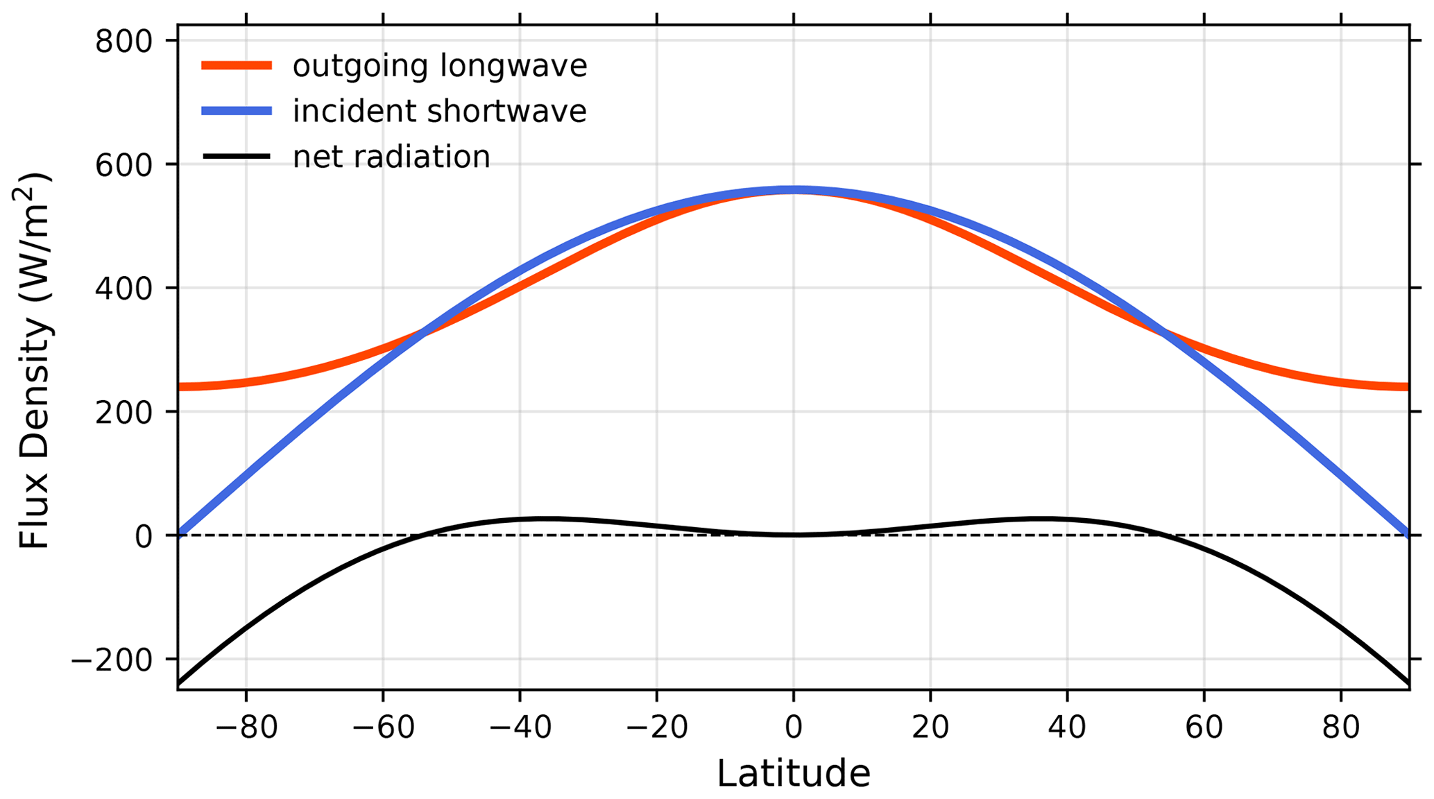
However, in computing the diabatic heating and cooling terms of stratospheric aerosols in Sect. 3, it will be both convenient and natural to have expressions for the flux densities of incoming shortwave (SW) and outgoing longwave (LW) broadbands, which are qualitatively consistent with the HSW equilibrium temperature field. We first define a global, zonally symmetric longwave flux density based on T_eq at the surface and then deduce a shortwave component by setting the total integrated global power equal to that of the longwave component. Both flux density profiles will be constant in time.

In both the Held and Suarez (1994) and HSW models, the radiative equilibrium temperature below 100 hPa is

$$\begin{array}{}\text{(2)}& \begin{array}{rl}{T}_{\text{eq}}(\mathit{\varphi },p)& =\text{max}\left[\right(\mathrm{200}\text{K}),[\left(\mathrm{315}\text{K}\right)-\left(\mathrm{60}\text{K}\right){\sin }^{\mathrm{2}}\mathit{\varphi }\\ & -\left(\mathrm{10}\text{K}\right)\log \left({\displaystyle \frac{p}{p_{\mathrm{0}}}}\right){\cos }^{\mathrm{2}}\mathit{\varphi }\left]{\left({\displaystyle \frac{p}{p_{\mathrm{0}}}}\right)}^{R_d/c_p}\right],\end{array}\end{array}$$

where $R_d/c_p=\mathrm{2}/\mathrm{7}$ is the ratio of the ideal gas constant and specific heat at constant pressure for dry air. At the reference pressure p₀=1000 hPa, the equation reduces to

$$\begin{array}{}\text{(3)}& T_{\text{eq}}\left(\mathit{\varphi },p_{\mathrm{0}}\right)=\mathrm{315}\text{K}-\left(\mathrm{60}\text{K}\right){\sin }^{\mathrm{2}}\mathit{\varphi }.\end{array}$$

We compute a longwave gray-body flux density I_LW from the Stefan–Boltzman law as

$$\begin{array}{}\text{(4)}& I_{\text{LW}}=\mathit{\sigma }{T}_{\text{surf}}^{\mathrm{4}}=\mathit{\sigma }{\left[\mathrm{315}\text{K}-\left(\mathrm{60}\text{K}\right){\sin }^{\mathrm{2}}\mathit{\varphi }\right]}^{\mathrm{4}},\end{array}$$

where σ is the Stefan–Boltzman constant. If desired, T_surf can be the actual surface temperature on the 2D surface mesh. We instead choose a simplified approach that is both analytic and static in time by approximating the surface temperature as Eq. (3). For incident shortwave radiation, we use a simple cosine form which vanishes at the poles, resembling equinox conditions and given by

$$\begin{array}{}\text{(5)}& I_{\text{SW}}=I_{\mathrm{0}}\cos \mathit{\varphi }.\end{array}$$

By integrating Eqs. (4) and (5) over the sphere, we find that a normalization parameter of I₀≈560 W m⁻² ensures that the total globally integrated power is in balance between I_LW and I_SW. We note that these radiative fluxes are considerably higher than the annual average solar insolation of the real Earth system. The primary reason for the enhanced values is that there is no attenuation of the upwelling longwave radiation by moisture, clouds, or other background constituents (excluding volcanic aerosols) in the HSW atmosphere. Including such an effect in the HSW configuration would be arbitrary and overly complicated. Further, we will show in Sect. 3 that the aerosol radiative forcing design has sufficient freedom in the number of tunable parameters to achieve the desired heating rates, without being preferential about the amplitudes of I_SW and I_LW.

The resulting flux profiles are shown in Fig. 2. This figure shows an energy deficit poleward of 55^∘ and a surplus equatorward, with maxima in the net flux at the middle latitudes. We emphasize that the shape of the flux profiles is the important aspect here and that balancing I_LW and I_SW is only being done for style and physical legibility. This “radiation” will be used only to control the heating and cooling rates imposed by injected aerosols, which will ultimately be subject to model tuning and will have no effect on mean atmospheric temperatures. The overall climate and energy balance is still controlled independently by the HSW temperature relaxation.

Figure 2 Longwave (Eq. 4), shortwave (Eq. 5), and net flux densities as functions of latitude.

3 The HSW-V volcanic forcing approach

We model radiative forcing by stratospheric aerosol injection events in the idealized HSW environment by directly forcing the temperature field using a standalone parameterization. This forcing is done without the need for intermediary aerosol or radiation models. While this approach could be generalized for any local injections of sulfur species into the atmosphere, the implementation used here is designed and tuned to produce a realistic representation of the 1991 eruption of Mt. Pinatubo. Specifically, our model describes the localized simultaneous injection of volcanic ash and sulfur dioxide (SO₂) with a specified vertical profile over a single model column. Decay of the SO₂ in turn leads to production of long-lived sulfate aerosols. These chemical species are implemented as “tracers” within EAMv2 (scalar mixing ratio quantities advected by the model's transport scheme) and contribute independently to local and surface temperature tendencies.

The strategy is to add together various ingredients as follows: (1) define volcanic sources (stratospheric injection), (2) define SO₂ sinks (sulfate aerosol production), (3) compute the aerosol optical depth (AOD) of each model column, and (4) increment the temperature tendency (local radiative heating by absorption and radiative surface cooling by AOD). Steps (1)–(4) are described in Sect. 3.1–3.4. Section 3.5 provides a brief summary of the model, a table of the model parameters, and notes on the parameter tuning strategy.

3.1 Tracer injection

We model the time tendency of each injected tracer species j (SO₂ and ash) as the sum of a source and a sink:

$$\begin{array}{}\text{(6)}& {\displaystyle \frac{\partial m_j}{\partial t}}=R\left(m_j\right)+f.\end{array}$$

R(m_j) is an exponential removal function with an e-folding timescale $\mathrm{1}/k_j$, and the source term f describes the spatial distribution of injection:

$$\begin{array}{}\text{(7)}& {\displaystyle }R\left(m_j\right)=-k_j{m}_j,\text{(8)}& {\displaystyle }f={\stackrel{\mathrm{̃}}{A}}_{j}T\left(t\right)H(\mathit{\varphi },\mathit{\lambda })V\left(z\right).\end{array}$$

The separable temporal, vertical, and horizontal dependencies are T(t), V(z), and H(ϕ,λ), respectively, where z is the geometric height and λ symbolizes the longitude. ${\stackrel{\mathrm{̃}}{A}}_j$ is a normalization parameter. This form is then discretized onto the model grid with horizontal column, vertical level, and time-step indices i, k, and n, respectively. We choose to model an injection uniformly distributed over a single column and time period of length δt. Explicitly, the “injection region” S is symbolized as

$$\begin{array}{}\text{(9)}& S=\mathit{\left\{}\right({\mathit{\varphi }}_i,{\mathit{\lambda }}_i,t_n\left)\right|{\mathit{\varphi }}_i={\mathit{\varphi }}_{i^{\prime }},{\mathit{\lambda }}_i={\mathit{\lambda }}_{i^{\prime }},t_{\mathrm{0}}\le t_n\le t_{\mathrm{0}}+\mathit{\delta }t\mathit{\}},\end{array}$$

where i^′ is the index of the injection column. The product of T(t_n) and H(ϕ_i,λ_i) in Eq. (8) is then replaced with an indicator function $I_{i,n}\equiv I(t_n,{\mathit{\varphi }}_i,{\mathit{\lambda }}_i)$, which is equal to one inside of S and equal to zero outside of S. The mass tendency is then

$$\begin{array}{}\text{(10)}& {\displaystyle \frac{\partial m_{j,i,k}}{\partial t}}=-k_j{m}_{j,i,k}+I_{i,n}{A}_{j}V\left(z_k\right).\end{array}$$

The source f for tracer j is normalized by the constant A_j, which scales the total injected mass to a known parameter M_j by

$$\begin{array}{}\text{(11)}& {\displaystyle }{M}_j=A_j\mathit{\delta }t\sum _{k}V\left(z_k\right)\text{(12)}& {\displaystyle }\Rightarrow A_j={\displaystyle \frac{M_j}{\mathit{\delta }t{\sum }_k{V}_k}},\end{array}$$

where we define V_k≡V(z_k). The normalization constant A_j is unique to the vertical grid configuration and converges to the normalization of the analytic form $A_j\to {\stackrel{\mathrm{̃}}{A}}_j$ with increasing resolution. This treatment avoids losing mass to numerical diffusion once the injected mass is placed on the model grid.

Rather than a mass tendency, the quantity required by EAMv2's physics interface is the tendency of the tracer mixing ratio $q_j\equiv m_j/m_{\text{atm}}$. If Δp_i,k is the local pressure thickness of the grid cell, g is the acceleration due to gravity and a_i is the column area, the air mass m_atm in this definition can be replaced using the hydrostatic equation, yielding

$$\begin{array}{}\text{(13)}& q_{j,i,k}=m_{j,i,k}{\displaystyle \frac{g}{\mathrm{\Delta }{p}_{i,k}{a}_i}}.\end{array}$$

Given Eqs. (10)–(13), the final expression implemented for the update of tracer j at column i, vertical level k, and time step n is

$$\begin{array}{}\text{(14)}& {\displaystyle \frac{\partial q_{j,i,k,n}}{\partial t}}={\displaystyle \frac{g}{\mathrm{\Delta }{p}_{i,k}{a}_i}}\left[-k_j{m}_{j,i,k}+I_{i,n}{\displaystyle \frac{M_j}{\mathit{\delta }t{\sum }_k{V}_k}}{V}_k\right].\end{array}$$

For the vertical dependence V(z), we follow Fisher et al. (2019) and assume a Gaussian distribution defined by a center of mass altitude (µ) and a geometrical standard deviation

$$\begin{array}{}\text{(15)}& V\left(z\right)=\exp \left(-{\displaystyle \frac{\mathrm{1}}{\mathrm{2}}}{\displaystyle \frac{(z-\mathit{\mu }{)}^{\mathrm{2}}}{(\mathrm{1.5}\text{km}{)}^{\mathrm{2}}}}\right).\end{array}$$

The profile deviation of 1.5 km is a compromise between Fisher et al. (2019) and the width of the parabolic injection profile of Stenchikov et al. (2021). In hydrostatic models such as E3SMv2, the height z is a diagnostic quantity. Therefore, the vertical profile needs to be computed at each time step. We inject both SO₂ and ash at the same height and with the same deviation, and we do not include a normalization coefficient in V(z), since A_j is already scaled by ∑_kV_k.

We tuned the center of mass altitude (µ) by ensuring that the sulfate tracer which eventually arises from the initial SO₂ injection settles in the lower stratosphere, between 20 and 25 km, consistent with estimates from aerosol transport models (Sheng et al., 2015) and forcing reconstructions (see the review in Sect. 2 of Toohey et al., 2016). As in previous works, we might expect to inject just above the tropical tropopause, near μ=17–18 km (Stenchikov et al., 2021; Fisher et al., 2019), and then allow the self-lofting process to carry the plume to a level of neutral buoyancy in the lower stratosphere. As per Stenchikov et al. (2021), this process is expected to be driven by a vertical velocity of w≈1 km d⁻¹ due to strong initial radiative heating rates of about 20 K d⁻¹ in the dense, fresh volcanic plume. After tuning the model with these considerations in mind, we use the even lower value of μ=14 km, which we found to result in a realistic settling altitude for the sulfate tracer distribution. The need for this exceptionally low injection height is due to an overly aggressive heating of the initial plume given our parameter choices, which is discussed further in Sect. 3.5 and Appendix C4.

Observations giving the total injected mass and e-folding time for SO₂ (25 d) and ash (1 d) for the Mt. Pinatubo eruption were estimated from satellite data and published in Guo et al. (2004a, b) and Barnes and Hofmann (1997). Table 1 provides the chosen parameter values. In particular, the model describes a 24 h injection of a plume centered on 14 km in the vertical and uniformly over a single column. We assume no background values for any of the injected species prior to the eruption, as in some other studies (e.g., Bekki and Pyle, 1994).

The remainder of the model formulation as presented in Sect. 3.2–3.4 is applied uniformly to each time step, and thus the temporal index n will be omitted for brevity. Optical depths and radiative forcings are computed identically for each tracer species, and so the tracer index j will also be omitted. Mixtures of multiple tracers j with varying radiative extinction coefficients will be reintroduced in Sect. 3.4.3.

Stenchikov et al. (2021)Guo et al. (2004a)Barnes and Hofmann (1997)Guo et al. (2004b)Guo et al. (2004a)Guo et al. (2004b)

Table 1 Model parameters. Parameters with the superscript † are tuned parameters. Parameters with the superscript ‡ are constrained by a data-driven calculation though are not necessarily free for tuning. Parameters without a superscript are observations and/or estimates directly from the literature. For information on the tuning, see Sect. 3.5 and Appendix C.

3.2 Sulfate formation

Once injected into the atmosphere, SO₂ follows an oxidation chain with an end product of sulfuric acid (H₂SO₄) that condenses with water vapor to form sulfate aerosol particles (Bekki, 1995). Stratospheric sulfate aerosols have an e-folding removal timescale of 1 year (Barnes and Hofmann, 1997) and are responsible for much of the heating that perturbs Earth's energy balance and atmospheric circulation after a stratospheric volcanic eruption (McCormick et al., 1995; Robock, 2002).

In fully coupled climate models, aerosol heating will be mediated by chemistry, radiation, and moist subgrid processes. Here, the same heating is rather modeled by a direct, analytic coupling of SO₂ to sulfate in a way inspired by the so-called “toy chemistry” of Lauritzen et al. (2015) and also seen in Toohey et al. (2016). Sulfate will evolve using Eq. (6), where the source term f exactly becomes the SO₂ sink $R\left(m_{{\mathrm{SO}}_{\mathrm{2}}}\right)$. The SO₂ removal rate $k_{{\mathrm{SO}}_{\mathrm{2}}}$ is then interpreted purely as a reaction rate, and the sulfate tendency mass is

$$\begin{array}{}\text{(16)}& {\displaystyle \frac{\partial m_{\text{sulf}}}{\partial t}}=-k_{\text{sulf}}{m}_{\text{sulf}}+\mathit{\nu }{k}_{{\text{SO}}_{\mathrm{2}}}{m}_{{\text{SO}}_{\mathrm{2}}}\end{array}$$

or, in terms of the mixing ratio on the computational grid,

$$\begin{array}{}\text{(17)}& {\displaystyle \frac{\partial q_{\text{sulf},i,k}}{\partial t}}=-k_{\text{sulf}}{q}_{\text{sulf},i,k}+\mathit{\nu }{k}_{{\mathrm{SO}}_{\mathrm{2}}}{q}_{{\mathrm{SO}}_{\mathrm{2}},i,k}.\end{array}$$

Here, the reaction weight ν encodes the net production of sulfate per unit mass of SO₂. While ν could be a tuning parameter of the model, we can inform a first choice from chemistry. Since the overall effect of the oxidation sequence yields one aerosol “particle” of sulfate per molecule of SO₂ (Bekki, 1995), ν will just be the ratio of the sulfate to the SO₂ molar mass. Though it is known from observation that sulfate particles vary in their composition across latitude, altitude, and season (Yue et al., 1994), depending on specific humidity and temperature, we make the simplifying assumption that all sulfate particles are 75 % H₂SO₄ by mass. The same assumption is made in Bekki (1995) and is suggested by observation (Rosen, 1971; Yue et al., 1994). Defining this percentage as f_acid=0.75 and the molar masses of H₂SO₄ and SO₂ as M(H₂SO₄) and M(SO₂), the reaction weighting is

$$\begin{array}{}\text{(18)}& \mathit{\nu }={\displaystyle \frac{M\left({\text{H}}_{\mathrm{2}}{\text{SO}}_{\mathrm{4}}\right)/f_{\text{acid}}}{M\left({\text{SO}}_{\mathrm{2}}\right)}}\approx {\displaystyle \frac{\mathrm{1}/\mathrm{0.75}\times \mathrm{98.079}\mathrm{g}{\mathrm{mol}}^{-\mathrm{1}}}{\mathrm{64.066}\mathrm{g}{\mathrm{mol}}^{-\mathrm{1}}}}=\mathrm{2.04}.\end{array}$$

This choice of ν results in a peak sulfate mass of about ∼ 28 Mt occurring approximately 2 months after injection, which is consistent with previous modeling efforts by, e.g., Bluth et al. (1997). In that study, however, the authors note that if we assume sulfate production to arise directly from SO₂ depletion, then the inferred sulfate loading does not coincide with observed 0.55 µm AOD anomalies after Pinatubo. Citing the AOD database of Sato et al. (1993), Bluth et al. (1997) show this peak AOD anomaly to occur nearer to 9 months than 2 months.

For this reason, Toohey et al. (2016) (who also modeled the SO₂→ sulfate conversion directly) decided to address this lag in the AOD anomaly by artificially inflating the SO₂ dissipation parameter to $k_{{\mathrm{SO}}_{\mathrm{2}}}=\mathrm{1}/\mathrm{180}$ d⁻¹. This change is said to represent the net timescale of all processes resulting in an increased global-mean AOD, beyond just the oxidation chain producing H₂SO₄, which may not be fully captured in this idealized description. In this way, they delay the peak sulfate loading, and thus the peak 0.55 µm AOD anomaly, from 2 months to 6 months post-injection. This figure is more consistent with the Pinatubo AOD anomaly time series constructed by the Chemistry-Climate Model Initiative (CCMI; Eyring et al., 2013).

Rather than following these findings of Bluth et al. (1997) and Toohey et al. (2016), we decide instead to retain the observed value of $k_{{\mathrm{SO}}_{\mathrm{2}}}=\mathrm{1}/\mathrm{25}$ d⁻¹. This choice causes the peak AOD anomaly to occur simultaneously with the sulfate loading near month 2, which is consistent with the 0.55 µm AOD results of the prognostic aerosol implementation of Brown et al. (2024) as well as observations of 0.6 µm AOD from the Advanced Very High Resolution Radiometer (AVHRR; Zhao et al., 2013; Heidinger et al., 2014). We verified that the difference in peak sulfate mass between our model and Toohey et al. (2016) is explained fully by the choice of $k_{{\mathrm{SO}}_{\mathrm{2}}}$ and not the reaction normalization ν.

3.3 Aerosol optical depth

A single aerosol species can contribute to extinction of transmitted radiation by absorption and scattering, the combined effect of which is expressed by a spatially varying extinction coefficient ${\mathit{\beta }}_e(x,y,z)$. Within a single model column, we will make the plane-parallel approximation, i.e., ${\mathit{\beta }}_e(x,y,z)\approx {\mathit{\beta }}_e\left(z\right)$. This coefficient can be further expanded as

$$\begin{array}{}\text{(19)}& {\mathit{\beta }}_e=b_e\mathit{\rho }=b_{e}q{\mathit{\rho }}_{\mathrm{atm}},\end{array}$$

where b_e is the mass extinction coefficient of the aerosol species, with dimensions of area per unit mass; ρ is the tracer mass density; and q is the mixing ratio. Consistent with Sect. 2.3, the extinction properties of each tracer species j will be modeled with respect to two broadbands: b_LW will be used for the extinction of LW radiation, which is assumed to be entirely absorption, and b_SW will be used for the extinction of SW radiation, which is assumed to be entirely scattering:

$$\begin{array}{c}{\displaystyle }{b}_{\text{LW}}\equiv \left(b_e\text{for the longwave band}\right),\\ {\displaystyle }{b}_{\text{SW}}\equiv \left(b_e\text{for the shortwave band}\right).\end{array}$$

For a column with a model top at z_top, the dimensionless SW AOD τ at a height z is obtained by vertically integrating the shortwave extinction:

$$\begin{array}{}\text{(20)}& \mathit{\tau }\left(z\right)=\underset{z}{\overset{z_{\text{top}}}{\int }}{\mathit{\beta }}_e\left(z^{\prime }\right)\mathrm{d}{z}^{\prime }=\underset{z}{\overset{z_{\text{top}}}{\int }}{b}_{\text{SW}}q\left(z^{\prime }\right){\mathit{\rho }}_{\mathrm{atm}}\left(z^{\prime }\right)\mathrm{d}{z}^{\prime }.\end{array}$$

On the model grid, this extinction becomes

$$\begin{array}{}\text{(21)}& {\displaystyle }{\mathit{\tau }}_{i,k}=\sum _{k^{\prime }<k}{b}_{\text{SW}}{q}_{i,k^{\prime }}{\mathit{\rho }}_{\text{atm},i,k^{\prime }}\mathrm{\Delta }{z}_{i,k^{\prime }}\text{(22)}& {\displaystyle }=\sum _{k^{\prime }<k}{b}_{\text{SW}}{\displaystyle \frac{q_{i,k^{\prime }}\mathrm{\Delta }{p}_{i,k^{\prime }}}{g}},\end{array}$$

where the pressure thickness Δp symbolizes the pressure difference between two neighboring model interface levels that surround the full model level with index k^′.

We assume that the indices k and k^′ decrease toward the model top (as in E3SMv2). We also define a shorthand for the cumulative SW AOD at the surface as ${\mathit{\tau }}_i\equiv \mathit{\tau }(z=\mathrm{0})$. After summing over k for this case, we have the usual result (Petty, 2006) that each remaining term is just the total column mass burden M_i of the tracer, scaled by the mass extinction coefficient b_SW and the column area a_i:

$$\begin{array}{}\text{(23)}& {\mathit{\tau }}_i=\sum _k{b}_{\text{SW}}{\displaystyle \frac{q_{i,k}\mathrm{\Delta }{p}_{i,k}}{g}}=\sum _k{b}_{\text{SW}}{\displaystyle \frac{q_{i,k}{m}_{atm,i,k}}{a_i}}=b_{\text{SW}}{\displaystyle \frac{M_i}{a_i}}.\end{array}$$

Hereafter, “AOD” will refer specifically to the column-integrated SW AOD defined in Eq. (23).

3.4 Radiative forcing

Injected stratospheric aerosols force the Earth system in two primary ways, i.e., (1) local heating of the stratosphere and (2) remote cooling of the surface. The presence of SO₂ and sulfate aerosols in the stratosphere induces local diabatic heating in the temperature field by absorption of upward-propagating longwave radiation (Kinne et al., 1992; Brown et al., 2024). After the 1991 Mt. Pinatubo eruption, this process resulted in a positive temperature anomaly of up to ∼ 2–4 K, peaking near 50–30 hPa (Rieger et al., 2020; Stenchikov et al., 1998; Labitzke and McCormick, 1992) and driven by a maximum net temperature change at a rate of ∼ 1 K per month during the initial period following the injection.

At the same time, increased aerosol optical depths of the vertical column decrease the flux density of shortwave solar radiation reaching the troposphere. This upper-level scattering of solar radiation contributed to an observed surface cooling of $\sim -\mathrm{0.5}$ K during the 2 years following the eruption of Mt. Pinatubo (Dutton and Christy, 1992; Self et al., 1993; Fyfe et al., 2013).

We model each of these heating effects by adding new forcing terms to the temperature field of the HSW atmosphere. Heating is applied in the stratospheric aerosol plume, and the lowest few model levels are cooled using the computation of the energy change that results from the attenuation of the flux densities I_LW and I_SW.

3.4.1 Local heating of the stratosphere

The local warming effect is modeled as an attenuation of upwelling longwave radiation with flux density I_LW defined in Eq. (4), computed for each model column using the plane-parallel Beer–Lambert law. To begin, the attenuated flux density after transmission through a particular slab with vertical bounds [z₀, z₁] is an integral of the extinction β_e, such as

$$\begin{array}{}\text{(24)}& I(z_{\mathrm{0}},z_{\mathrm{1}})=I_{\text{LW}}\text{exp}\left(-\underset{z_{\mathrm{0}}}{\overset{z_{\mathrm{1}}}{\int }}{\mathit{\beta }}_e\left(z^{\prime }\right)\mathrm{d}{z}^{\prime }\right).\end{array}$$

Here we assume that z₀ is the lowest extent of the aerosol plume, and there has been no attenuation between z=0 and z=z₀. In this case, the power per unit area absorbed by the slab is

$$\begin{array}{}\text{(25)}& \mathrm{\Delta }I=I_{\text{LW}}-I(z_{\mathrm{0}},z_{\mathrm{1}}).\end{array}$$

If we consider another slab located immediately above z₁, on [z₁, z₂], then the incident flux is no longer I_LW but rather I(z₀,z₁), and the power per unit area absorbed is

$$\begin{array}{}\text{(26)}& \begin{array}{rl}\mathrm{\Delta }I& =I(z_{\mathrm{0}},z_{\mathrm{1}})-I(z_{\mathrm{1}},z_{\mathrm{2}})\\ & =I_{\text{LW}}\text{exp}\left(-\underset{z_{\mathrm{0}}}{\overset{z_{\mathrm{1}}}{\int }}{\mathit{\beta }}_e\left(z^{\prime }\right)\mathrm{d}{z}^{\prime }\right)\\ & \left[\mathrm{1}-\text{exp}\left(-\underset{z_{\mathrm{1}}}{\overset{z_{\mathrm{2}}}{\int }}{\mathit{\beta }}_e\left(z^{\prime }\right)\mathrm{d}{z}^{\prime }\right)\right].\end{array}\end{array}$$

This form generalizes to an arbitrary slab on [z_n, z_n+1] as

$$\begin{array}{}\text{(27)}& \begin{array}{rl}\mathrm{\Delta }I& =I(z_{n-\mathrm{1}},z_n)-I(z_n,z_{n+\mathrm{1}})\\ & =I_{\text{LW}}\text{exp}\left(-\underset{z_{\mathrm{0}}}{\overset{z_n}{\int }}{\mathit{\beta }}_e\left(z^{\prime }\right)\mathrm{d}{z}^{\prime }\right)\\ & \left[\mathrm{1}-\text{exp}\left(-\underset{z_n}{\overset{z_{(n+\mathrm{1})}}{\int }}{\mathit{\beta }}_e\left(z^{\prime }\right)\mathrm{d}{z}^{\prime }\right)\right].\end{array}\end{array}$$

Discretizing these integrals onto the vertical grid with levels k and column i yields

$$\begin{array}{}\text{(28)}& \begin{array}{rl}\mathrm{\Delta }{I}_{i,k}=& I_{\text{LW}}\text{exp}\left(-\sum _{k^{\prime }>k}{b}_{\text{LW}}{\displaystyle \frac{q_{i,k^{\prime }}\mathrm{\Delta }{p}_{i,k^{\prime }}}{g}}\right)\\ & \left[\mathrm{1}-\text{exp}\left(-b_{\text{LW}}{\displaystyle \frac{q_{i,k}\mathrm{\Delta }{p}_{i,k}}{g}}\right)\right],\end{array}\end{array}$$

where the argument of the leftmost exponent sums over all levels k^′ which are below level k. The effect here is that aerosols lower in the vertical column “shadow” those above, decreasing the power of incident radiation available for absorption. In this way, the peak of the local aerosol heating may lie below the actual density peak of the plume.

The absorbed power per unit area is then translated to a heating rate per unit mass s and finally to an associated temperature tendency ΔT, with the assumption that all of the absorbed radiation is perfectly converted to heat. If the flux densities are given in Watt per square meter, then, by dimensional analysis,

$$\begin{array}{}\text{(29)}& {\displaystyle }{s}_{i,k}={\displaystyle \frac{a_i\mathrm{\Delta }{I}_{i,k}}{m_{i,k}}}{\displaystyle \frac{\text{J}}{\text{kg s}}}\text{(30)}& {\displaystyle }\Rightarrow \mathrm{\Delta }{T}_{i,k}={\displaystyle \frac{\mathrm{1}}{c_p}}{\displaystyle \frac{a_i\mathrm{\Delta }{I}_{i,k}}{m_{i,k}}}{\displaystyle \frac{\text{K}}{\text{s}}}.\end{array}$$

This temperature tendency is always positive and will be imposed on the grid cell at (i,k) for each tracer at each time step.

3.4.2 Cooling of the surface

The surface cooling is modeled as an AOD attenuation of incident radiation with flux density I_SW, as defined in Eq. (5). We begin with a form analogous to Eq. (24), where the vertical slab on [z₀,z₁] is replaced with the entire vertical column above position z on [z,z_top]. The integral term in parentheses is then exactly the AOD as given in Eq. (20). The attenuation is thus

$$\begin{array}{}\text{(31)}& I\left(z\right)=I_{\text{SW}}\text{exp}\left(-\underset{z}{\overset{z_{\text{top}}}{\int }}{\mathit{\beta }}_e\left(z^{\prime }\right)\mathrm{d}{z}^{\prime }\right)=I_{\text{SW}}{e}^{-\mathit{\tau }\left(z\right)}.\end{array}$$

With the notation used in Eq. (23), the deficit flux density after attenuation by the aerosol over the full height of the atmosphere in a single model column i is

$$\begin{array}{}\text{(32)}& \mathrm{\Delta }{I}_i=I_{\text{SW}}\left(e^{-{\mathit{\tau }}_i}-\mathrm{1}\right).\end{array}$$

That is, a deficit energy density of ΔI_i W m⁻² is imposed at the surface. For a model column at the Equator with τ=0.2, this form gives $\mathrm{\Delta }I\approx -\mathrm{100}$ W m⁻², which is roughly consistent with the observed broadband solar transmission deficits of ∼ 20 % at Mauna Loa, Hawaii, in the months following Pinatubo (Self et al., 1993; see their Fig. 9). With AODs of τ≈4, the shortwave attenuation saturates (all available incident radiation has scattered).

The attenuation is next translated to a cooling rate per unit mass s and an associated temperature tendency ΔT. Since the HSW atmosphere simulates no land–atmosphere coupling processes, we employ a very simple representation of the conduction and convection that would, in reality, be responsible for communicating an energy deficit at the ground to the atmospheric surface layer. We imagine that all of the energy lost over the column heats the planetary surface, which in turn transfers heat to the atmosphere by a function F with some efficiency ζ:

$$\begin{array}{}\text{(33)}& s_{i,k}=\mathit{\zeta }F\left(\mathrm{\Delta }{I}_i\right).\end{array}$$

The heat transfer “efficiency” ζ should be considered a catch-all for any surface–atmosphere coupling effects which we do not model, and it is treated as a tuning parameter for the magnitude of atmospheric surface cooling (see Sect. 3.5). As in the local heating treatment of the previous section, the function F can be obtained by dimensional analysis:

$$\begin{array}{}\text{(34)}& {\displaystyle }{s}_{i,k}=\mathit{\zeta }{\displaystyle \frac{a_i\mathrm{\Delta }{I}_i}{{\stackrel{\mathrm{̃}}{m}}_i}}{\displaystyle \frac{\text{J}}{\text{kg s}}}\text{(35)}& {\displaystyle }\Rightarrow \mathrm{\Delta }{T}_{i,k}=\mathit{\zeta }{\displaystyle \frac{\mathrm{1}}{c_p}}{\displaystyle \frac{a_i\mathrm{\Delta }{I}_i}{{\stackrel{\mathrm{̃}}{m}}_i}}{\displaystyle \frac{\text{K}}{\text{s}}},\end{array}$$

where ${\stackrel{\mathrm{̃}}{m}}_i$ is the mass of air in the lowest κ model levels of column i over which the cooling is to be applied. If we apply the cooling only to the lowest model level with κ=K, then

$$\begin{array}{}\text{(36)}& {\stackrel{\mathrm{̃}}{m}}_i=m_{i,K}\end{array}$$

and otherwise

$$\begin{array}{}\text{(37)}& {\stackrel{\mathrm{̃}}{m}}_i=\sum _{k=K}^{K-(\mathit{\kappa }-\mathrm{1})}{m}_{i,k}.\end{array}$$

In this way, the net cooling (total energy loss over unit time) is conserved as the parameter κ is increased, and the cooling per unit mass is “diluted”. The choice of κ will effectively encode whatever missing physical mechanisms would otherwise communicate the cooling higher into the vertical column. For κ>1, ΔT_i,k is a 3D quantity, while ΔI_i and τ_i are always 2D quantities. In Table 1, rather than setting κ directly, we set $\stackrel{\mathrm{̃}}{\mathit{\delta }z}$, or the height above the surface in meters where the cooling should be applied, from which κ is inferred given the vertical discretization.

3.4.3 Generalization to mixtures of tracer species

When multiple tracer species j are present (SO₂, ash, sulfate), the total radiative heating is not derived from a simple sum of the ΔT solutions found over the preceding sections. Rather, it is the total extinction which is determined by additive extinction coefficients:

$$\begin{array}{}\text{(38)}& {\mathit{\beta }}_e=\sum _j{\mathit{\beta }}_{e,j}=\sum _j{b}_{e,j}{m}_j.\end{array}$$

In this case, the total AOD of Eq. (23) becomes

$$\begin{array}{}\text{(39)}& \begin{array}{rl}{\mathit{\tau }}_i& =\sum _k\sum _j{b}_{\text{SW},j}{\displaystyle \frac{q_{j,i,k}\mathrm{\Delta }{p}_{i,k}}{g}}\\ & =\sum _j{b}_{\text{SW},j}{\displaystyle \frac{M_{j,i}}{a_i}}=\sum _j{\mathit{\tau }}_{j,i}.\end{array}\end{array}$$

For the total longwave heating, the expression is somewhat more complicated. Equation (28) becomes

$$\begin{array}{}\text{(40)}& \begin{array}{rl}\mathrm{\Delta }{I}_{i,k}=& I_{\text{LW}}\text{exp}\left(-\sum _j\sum _{k^{\prime }>k}{b}_{\text{LW},j}{\displaystyle \frac{q_{j,i,k^{\prime }}\mathrm{\Delta }{p}_{i,k^{\prime }}}{g}}\right)\\ & \left[\mathrm{1}-\text{exp}\left(-\sum _j{b}_{\text{LW},j}{\displaystyle \frac{q_{j,i,k}\mathrm{\Delta }{p}_{i,k}}{g}}\right)\right].\end{array}\end{array}$$

Here, each grid cell has an incident flux density that has already been attenuated by all species j underneath it, and so the total attenuation is not simply a sum of j separate evaluations of ΔI.

3.5 Model summary and parameter tuning

Figure 3 provides a summary of the important equations developed in the previous subsections, and Table 1 gives the chosen parameter values. Some parameter values are taken directly from observations or previous works in the literature, while others are derived quantities. Five parameters are tuning parameters, i.e., the longwave mass extinction coefficients for SO₂, sulfate, and ash; the maximum height of the forced surface cooling; and the surface heat transfer efficiency.

The longwave attenuation mechanism of the model is tuned to produce realistic stratospheric heating rates by sulfate aerosols. The mass extinction coefficient b_LW for sulfate is instrumental in tuning the long-term mean temperature anomalies. We note that, while we refer to this heating mechanism specifically as a “longwave attenuation”, the tuning process implicitly accounts for heating contributions from the near-infrared radiation as well (see Appendix C3). Not as obvious is the importance of b_LW for the very short-lived ash tracer. Though radiative forcing by ash does not directly contribute to the eventual stratospheric temperature anomalies, it does control the mechanism by which the aerosols are delivered to the lower stratosphere (Stenchikov et al., 2021). The lofting speed of the dense, fresh plume will be controlled by the aggressive heating of ash, which is the dominant component of the initial injection. As such, the mass extinction coefficient for ash serves as the main tuning parameter which controls the settling height of the aged aerosols. Meanwhile, SO₂ participates in both the initial lofting of the plume and the short-term temperature anomalies for the first couple of months. This behavior by SO₂ creates some degeneracy in the longwave extinction tuning parameters, which could be avoided with a slight modification; see Appendix C4 for a discussion.

The shortwave mass extinction coefficients b_SW do not play the same role in tuning the surface cooling. Instead, we simply constrain the b_SW of each species to yield an AOD representative of post-Pinatubo zonal-mean observations. During the months and years following the eruption, these values peaked near 0.2–0.5 (Toohey et al., 2016; Mills et al., 2016; Stenchikov et al., 2021; Dutton and Christy, 1992; Stenchikov et al., 1998). Tuning the magnitude of surface cooling is then passed on to the efficiency parameter ζ.

A description of the actual tuning process, as well as recommendations for tuning the model on different simulation grids and varying aerosol injection scenarios, can be found in Appendix C.

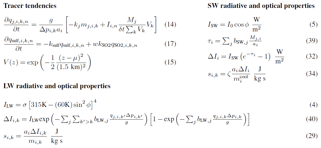
Figure 3 Summary of the important model equations controlling the tracer injection and removal, together with radiative and optical properties for the tracers in shortwave and longwave broadbands. See the equation numbers in the text for explanations. The SW and LW equations are written for a mixture of tracer species j at a fixed time step n. Values for the parameters are given in Table 1.

4 Implementation in E3SMv2

4.1 Ensemble generation

We explored two different ensemble generation strategies, which are characterized by “high-variability” (HV) or “limited-variability” (LV) sets of initial conditions. Both strategies appear in the literature, but they are not often explicitly named and compared.

In the HV strategy, ensemble member initial conditions are sampled from a base run of the HSW climate (described in Sect. 2) at an interval which produces independent atmospheric states. The choice of this time interval is unique to the model configuration. In making this determination, we follow the methodology of Gerber et al. (2008). In short, an index measuring the dynamical process which sets the upper bound on low-frequency variability in the model is defined, and the time that it takes for the autocorrelation of this index to vanish is found. At that time, we consider the initial condition to have been “forgotten”. For the HSW forcing, no seasonal cycle or ocean process is imposed, and so the upper-bound variability timescale is set by positional variations of the extratropical jets, encoded as the annular-mode index (defined in Gerber et al., 2008).

For a standard HS94 forcing on a ∼ 1° pseudospectral grid, Gerber et al. (2008) showed the annular-mode index autocorrelation to vanish by days 90–100. Lower-resolution grids had progressively longer timescales. We found that this autocorrelation was ∼ 0.1 by day 90 for the HSW atmosphere on the ne16pg2 grid in E3SMv2, only slowly converging thereafter to zero by day ∼ 250. Compromising on these diminishing returns for efficiency, our HV ensembles are generated by sampling initial states from a base run every 90 d. Volcanic injections can then begin at any point in the individual member integrations.

In the LV strategy, all ensemble members are initialized with an identical state, which is subjected to a random grid-point-level temperature perturbation of $\mathrm{1}\times {\mathrm{10}}^{-\mathrm{4}}$ K. We then wait some amount of time before enabling the volcanic injections. During this pre-injection period, the members will diverge from one another as dynamical feedbacks seeded by the initial temperature perturbations grow. In our experiments, waiting 75 d produced ensemble member background states that are more qualitatively similar in their zonally averaged flow but that exhibit synoptic-scale variations.

Note that the two timescales quoted above in the generation of the HV and LV ensembles are distinct and should not be confused. In the former case, the initial conditions lie 90 d apart from one another, while in the latter case the perturbed initial conditions evolve together but slowly diverge for a period of 75 d.

With enough members, the HV ensemble mean will show the average atmospheric response to our volcanic forcing independent of the background state. Meanwhile, an LV ensemble mean will show the robust response to a particular state, at least for the initial plume evolution. Eventually, the LV members will diverge and will be statistically similar to the HV ensemble once the aerosol distribution approaches zonal symmetry. Thus, an LV ensemble is perhaps most interesting to studies of this early phase.

Figure 4 shows a snapshot of a five-member volcanic injection ensemble at 8 d post-injection for the HV and LV ensemble generation strategies. The differences seen here are principally due to the fact that the HV ensemble samples strongly varying states of the northern polar jet, while the bulk aerosol transport of the plumes of the LV ensemble follow each other more closely. Also shown are time histories of the averaged zonal-mean zonal wind within 20° in latitude of the eruption site (from 5° S to 35° N) at 50 hPa for all the ensemble members, demonstrating the difference between the background HV and LV states.

Figure 5 displays the zonal mean of the initial conditions for temperature and zonal wind for ensemble members ens01, ens03, and ens05 for the HV case. These states show the qualitative spread in independent states sampled from an evolving HSW atmosphere, the most notable differences being the balance between (or collapse of) the polar jets and the strength of the stratospheric equatorial easterlies. Note that the zero contour rises steeply from the tropical to midlatitude regions, and thus the initial transport of a plume for a fixed height will vary strongly with latitude and will also be particularly sensitive to movements of the jet stream. The combination of the chosen initial condition and the parameter configuration given in Table 1 results in the lower tail of the initial injection distributions catching westerlies, while most of the mass enters the stratosphere and travels east. Note that all of the initial conditions for the LV case were based on perturbations of the HV ensemble member ens05 (Fig. 5c).

For the purposes of the present work, the model results of Sect. 4.2 are shown only for a HV ensemble. We encourage future studies using this model to present their ensemble generation methods in these terms.

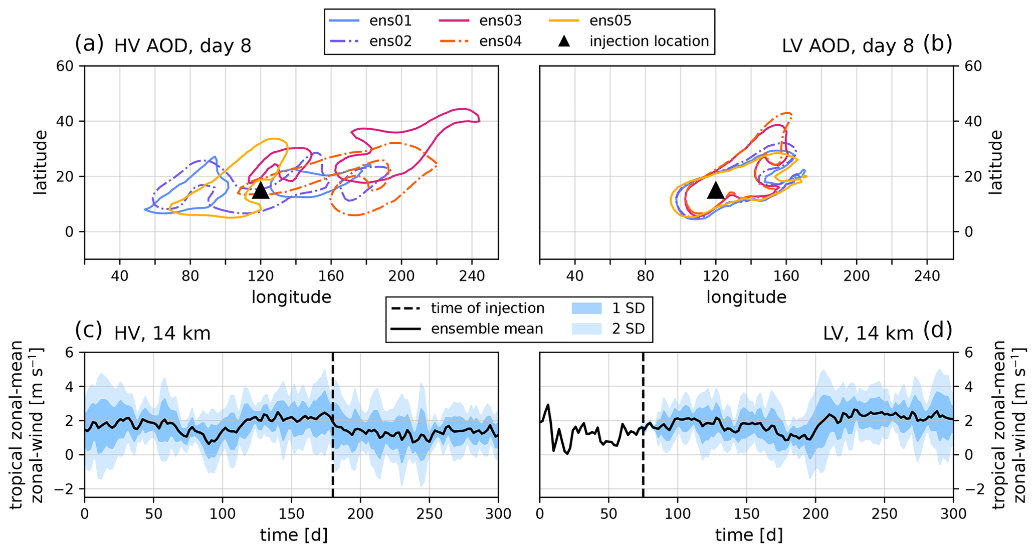
Figure 4 (a) AOD 0.5 contours for five HV ensemble members at 8 d post-injection. Each ensemble member is given a unique color, and their line styles alternate for visual clarity. (b) Identical to panel (a) but for five LV ensemble members. (c) Zonal-mean zonal wind averaged over a tropical region bracketing the injection site, from 5° S to 30° N at 50 hPa, for the HV ensemble. The bold black line shows the ensemble mean. Dark and light blue shadings show 1 and 2 standard deviations, respectively. The black vertical dashed line shows the time of injection (day 180). (d) Identical to panel (c) but for the LV ensemble, with injection at day 75.

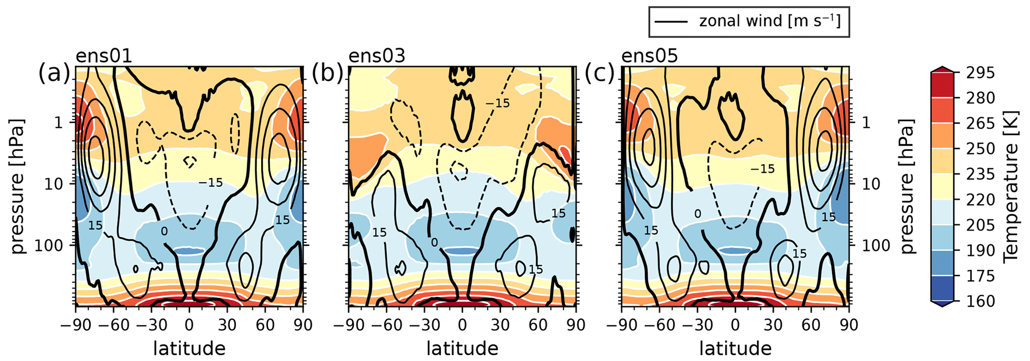
Figure 5 Zonal mean of the initial condition for ensemble members ens01, ens03, and ens05 for the HV ensemble (corresponding to the solid-line AOD distributions of Fig. 4). Temperature is shown on the color scale with intervals of 15 K and zonal wind in black contours with intervals of 15 m s⁻¹. The 0 m s⁻¹ contour in the zonal wind is shown in bold, and negative contours are dashed.

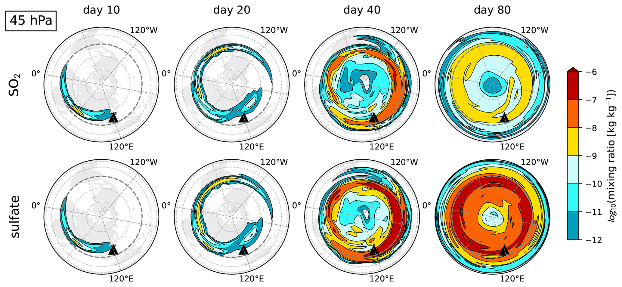
Figure 6 SO₂ (a) and sulfate aerosol (b) mixing ratios (kg tracer)(kg dry air)⁻¹ for a single ensemble member at the 45.67 hPa model level, displayed with a logarithmic scale. The columns from left to right correspond to 10, 20, 40, and 80 d post-injection. The data are plotted on a Lambert azimuthal equal-area projection extending from the North Pole to 60° S, where continental land masses are shown only for spatial reference (our model features no topography or land processes). A 30°×30° grid is drawn in dashed lines, with the Equator in bold dashed line. The injection location is marked with a black triangle.

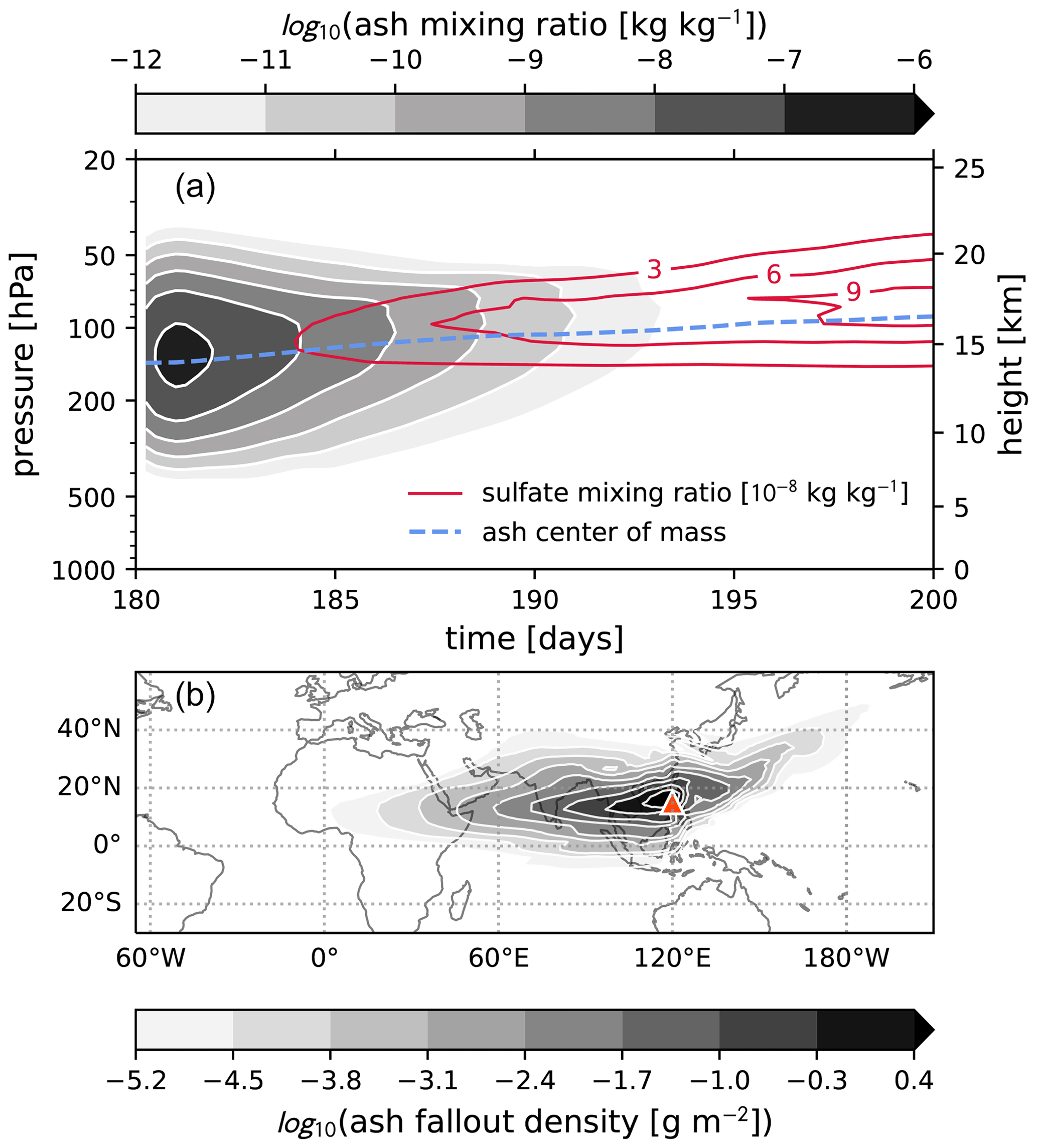
Figure 7 Evolution of the ash plume. (a) The zonal-mean and ensemble-mean logarithmic ash mixing ratios, averaged over all latitudes within 20° of the injection (from 5° S to 35° N). The dashed blue line shows the rising center of mass of the ash, and the solid red contours show the sulfate mixing ratios in intervals of 3×10⁸. The eruption occurs at day 180. (b) The cumulative sum of removed (“fallout”) stratospheric ash R(m_ash) over days 0 through 20 post-injection, together with all grid cells above 100 hPa, for a single ensemble member. The values are logarithmically scaled densities (g m⁻²). The red triangle marks the position of the volcanic injection. Continental land masses are shown only for spatial reference (our model features no topography or land processes).

4.2 Discussion of the results

We ran a five-member HV ensemble (Sect. 4.1) of E3SMv2 simulations subject to the modified idealized HSW physics (Sect. 2, Appendix A). A volcanic injection of SO₂ and ash (Sect. 3) occurs at day 180 with the parameter configuration of Table 1. Figure 6 shows the transport of the SO₂ and sulfate aerosol plumes at the 45 hPa model level for days 10, 20, 40, and 80 for the single ensemble member ens01. At this altitude, the dominant transport is driven by the easterly winds of the tropical stratosphere (see Fig. 1). By day 20 the plume has circled the globe, and by day 40 the plume has reached the North Pole. Also during this time, both SO₂ and sulfate concentrations have risen for this fixed vertical level. For SO₂, this effect is purely driven by vertical transport (our model contains no gravitational settling of any tracer species, and so all species will dynamically loft as long as heating is present), while for sulfate this effect is a combination of transport and actual aerosol production. By day 80, the tracer distributions are well-mixed in the tropical and midlatitude regions, and increasingly more SO₂ has been converted to sulfate.

Figure 7 provides a detailed view of the ash plume evolution over the first 20 d of the simulation. Panel (a) shows the zonal-mean ash mixing ratios as a function of time and pressure, averaged over a 20° band centered on the injection in latitude, from 5° S to 35° N. By day 12, the zonal-mean ash mixing ratios in this region have dissipated below 10⁻¹². Also shown for reference is the growing sulfate plume, which is just starting to be produced by SO₂ conversion. Panel (b) shows the total amount of ash removed from the stratosphere over the same time period (g m⁻²). That is, we are plotting the cumulative sum of the removal function R(m_ash) (Eq. 7) over all grid cells above 100 hPa, from days 180 through 200. Our model does not actually implement gravitational settling of ash, though our simple removal process can be thought of as an accumulated “fallout”. Thus, this distribution shows both the extent and history of the ash plume after 20 d.

Figure 8 displays the evolution of the zonal-mean AOD as a function of latitude and time as well as the imposed radiative cooling rate at the surface (K d⁻¹) by SW extinction. The AOD peaks at 0.3 near 15° N after 1 month, and by day 90 post-injection, zonal-mean optical depths of 0.1 reach the North Pole. Figure 9 shows the zonal-mean distribution of sulfate and the local stratospheric heating rate by LW absorption as a 30 d time average over days 60 through 90 post-injection. The aerosol density and heating rates coincide with one another in the tropics, while at higher latitudes the heating rate distribution develops strong meridional gradients that the sulfate mixing ratio does not. These gradients are an imprint of the LW radiation profile of Fig. 2, which is minimized at the poles.

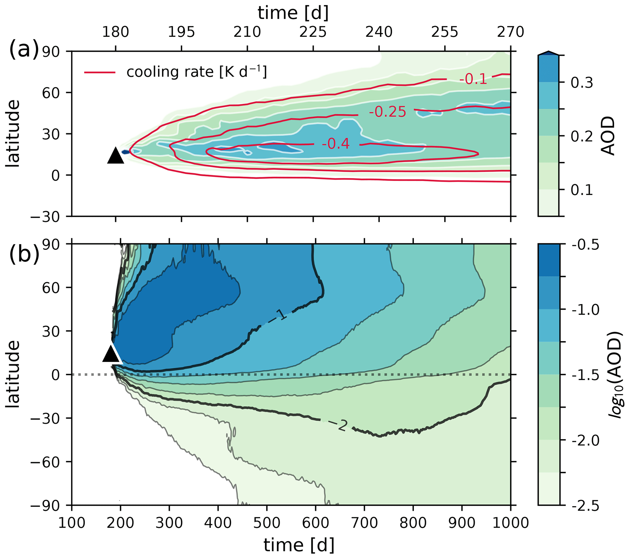
Figure 8 (a) Zonal-mean AOD in the latitude–time plane for the first 90 d post-injection. Overplotted in solid red contours is the cooling rate imposed on the lowest model level by shortwave extinction every 0.15 K d⁻¹. (b) Logarithmic zonal-mean AOD over 1000 d. The 0.1 and 0.001 AOD lines are in bold. Cooling rates are not overplotted in this panel. The faint dotted line shows the Equator, and the black triangle shows the time and latitude of the injection.

Several features of the HSW general circulation are shown in Figs. 8 and 9. A realistic tropopause is formed by the inversion of the equilibrium temperature T_eq near 130 hPa in the tropics. At the same time, the shape of T_eq at the lowest model levels mimics unequal solar insolation of the surface, driving convection in the tropical troposphere. Together, these effects give rise to upper-level divergence at the tropical tropopause and subsidence in the subtropics. The resulting Hadley cell can be seen in the sulfate distribution tail descending to the surface south of 30° N. The meridional transport of the zonally averaged tracer distribution, however, appears not to be hemispherically symmetric, with most of the aerosol population remaining in the Northern Hemisphere.

For the Mt. Pinatubo eruption, relative hemispheric symmetry of the AOD and temperature signal is established much more rapidly in both observations (Stenchikov et al., 1998; Mills et al., 2016) and more realistic models (Mills et al., 2016; Stenchikov et al., 2021; Ramachandran et al., 2000; Karpechko et al., 2010; Brown et al., 2024). This hemispheric symmetry is imposed because, in reality, the mean meridional circulation is characterized during the solstice months by a strong winter hemisphere Hadley cell, a relatively weak cell in the summer hemisphere, and a convergence zone north of the Equator (Schneider et al., 2014), driven by the seasonal cycle (Schneider, 2006) as well as asymmetry in the northern and southern land–sea distribution (Cook, 2003). During the Northern Hemisphere summer of July 1991, the upper-level diverging branch of the southern cell would have readily facilitated cross-equatorial transport of lower-stratospheric aerosols (Hoskins et al., 2020). All of these features are absent from our axisymmetric model, where any air masses in the upper troposphere or above will essentially always diverge from the Equator. To see this flow feature, the HSW Hadley cells are visualized using the Stokes streamfunction ψ(ϕ,p) in Fig. 9. Following previous studies (Oort and Yienger, 1996; Cook, 2003; Pikovnik et al., 2022), the ψ function is defined by a vertical integration of the zonally averaged meridional wind $\stackrel{\mathrm{‾}}{v}$ as

$$\begin{array}{}\text{(41)}& \mathit{\psi }(\mathit{\varphi },p)={\displaystyle \frac{\mathrm{2}\mathit{\pi }a\cos \mathit{\varphi }}{g}}\underset{\mathrm{0}}{\overset{p}{\int }}\stackrel{\mathrm{‾}}{v}(\mathit{\varphi },p^{\prime })\mathrm{d}{p}^{\prime },\end{array}$$

where a symbolizes Earth's radius. At a position in pressure and latitude, ψ gives the mean meridional mass transport over the entire stratospheric column above. Thus, positive (negative) peaks in the streamfunction distribution indicate clockwise (counterclockwise) circulation in the zonal average. The HSW streamfunction is anti-symmetric about the Equator, more closely resembling an equinox state in nature.

These conclusions about the mean tropospheric circulation can be expressed more generically for the stratospheric mass transport by way of a transformed Eulerian mean (TEM) analysis. Following the specific TEM framework presented in Gerber and Manzini (2016) based on Andrews et al. (1987), we computed residual velocities in the meridional plane for the HSW atmosphere with no volcanic injections. The 5-year average states of the residual velocities between 100 hPa and the model top near 0.1 hPa are presented in Appendix B. This residual circulation is essentially the HSW analog of the Brewer–Dobson circulation (BDC), which describes the global mass circulation through the stratosphere (see, e.g., Butchart, 2014, for a detailed review). Figure B1 shows two symmetric overturning circulation features from Equator to pole in each hemisphere, characterized by tropical upwelling, a midlatitude surf zone, and polar subsidence. This symmetry is markedly different from the average residual circulation of the Northern Hemisphere summer in nature, which sees a single southward pole-to-pole mass transport in the stratosphere (Butchart, 2014). Thus, the volcanic aerosol distribution as manifest in HSW-V remains primarily in the Northern Hemisphere, unlike the historical Mt. Pinatubo event. This circulation pattern is much more reminiscent of the equinox condition of the BDC. Specifically, the streamfunction presented in Fig. B1 is in good qualitative agreement with the observed residual streamfunction during the spring of 1992 following the historical Mt. Pinatubo eruption (Eluszkiewicz et al., 1996). Similarly, the meridional and vertical residual velocities are in qualitative agreement with those derived from the multi-reanalysis mean presented in Abalos et al. (2021) and the reanalysis springtime means in Fujiwara et al. (2022) (their Chap. 11). We note that, if a solstice condition is desired in the global circulation for future studies with this model, it would be straightforward to replace the HSW equilibrium temperature T_eq with a different one designed for that purpose, as in Polvani and Kushner (2002).

Finally, we quantify impacts by the volcanic aerosol forcing on the atmospheric state by atmospheric variable anomalies. Anomalies are defined as the grid-point-level arithmetic differences between a particular run (or ensemble mean) and the time average of a volcanically quiescent reference simulation. For this reference run, we use a 10-year run of the spun-up HSW atmosphere with no volcanic forcing, which is shown in Fig. 1b. Figure 10 shows the resulting ensemble-mean global-mean temperature anomaly as a function of pressure for 1000 d. The temperature anomaly peaks near 2 K at day 120 post-eruption in the stratosphere near 50 hPa, while the surface (lowest model level) anomaly peaks near −1 K. Note that the surface temperature anomalies exhibit much more noise than those in the stratosphere. In particular, we found that the stratospheric temperature anomaly is positive for any individual ensemble members, whereas the negative surface cooling anomaly is often significant (nonzero to at least 1 standard deviation) only in the ensemble mean.

Also shown in Fig. 10 are the total (globally integrated) tracer mass time series for SO₂ and sulfate as well as the vertical center of mass (COM) of the tropical stratospheric component of the sulfate distribution. The latter is simply defined as a subset of sulfate which remains above the peak of the vertical injection profile at 14 km or ∼ 130 hPa and within 20° of the injection at latitudes from 5° S to 35° N. This sulfate subset is the component of the plume most sensitive to radiative heating and is thus largely responsible for the global-mean stratospheric temperature anomaly (see Fig. 9).

4.3 Computational expense

Activating our scheme in E3SMv2 involves minimal computational overhead. We observed that a ne16pg2 HSW simulation with the volcanic parameterizations turned off runs at 175 simulated model years per wall-clock day (SYPD) executing on 384 processes (16 physics columns per process) on the Perlmutter supercomputer at the National Energy Research Scientific Computing Center (NERSC). This is equivalent to 52.6 core hours (or process-element hours) per simulated year, or “pe-h yr⁻¹”. With the same specifications, turning on the volcanic parameterizations reduces the throughput to 58.7 pe-h yr⁻¹, a decrease of ∼ 10 %.

This performance is in contrast to expensive prognostic aerosol implementations in coupled climate models, which often involve modal aerosol size distributions, more detailed radiative bands, and aerosol interactions with an inventory of other chemical species which must also be transported. For comparison, Brown et al. (2024) found 5395 pe-h yr⁻¹ when executing their prognostic stratospheric aerosol implementation on the higher-resolution ne30pg2 grid in a nudged atmosphere-only configuration of E3SMv2 on the Cheyenne machine at the National Center for Atmospheric Research (NCAR). For a fully coupled configuration of E3SMv2, Brown et al. (2024) found 9898 pe-h yr⁻¹, also on the ne30pg2 grid. Assuming that increasing the resolution from ne16pg2 to ne30pg2 involves a reduction in pe-h yr⁻¹ by a factor of 8, our model is ∼ 11 times faster and ∼ 21 times faster than atmosphere-only and fully coupled E3SMv2 simulations, respectively. The assumed factor of 8 comes from the fact that, when reducing both horizontal dimensions by a factor of 2, the time step must also be halved according to the Courant–Friedrichs–Lewy (CFL) condition of the dynamical core.

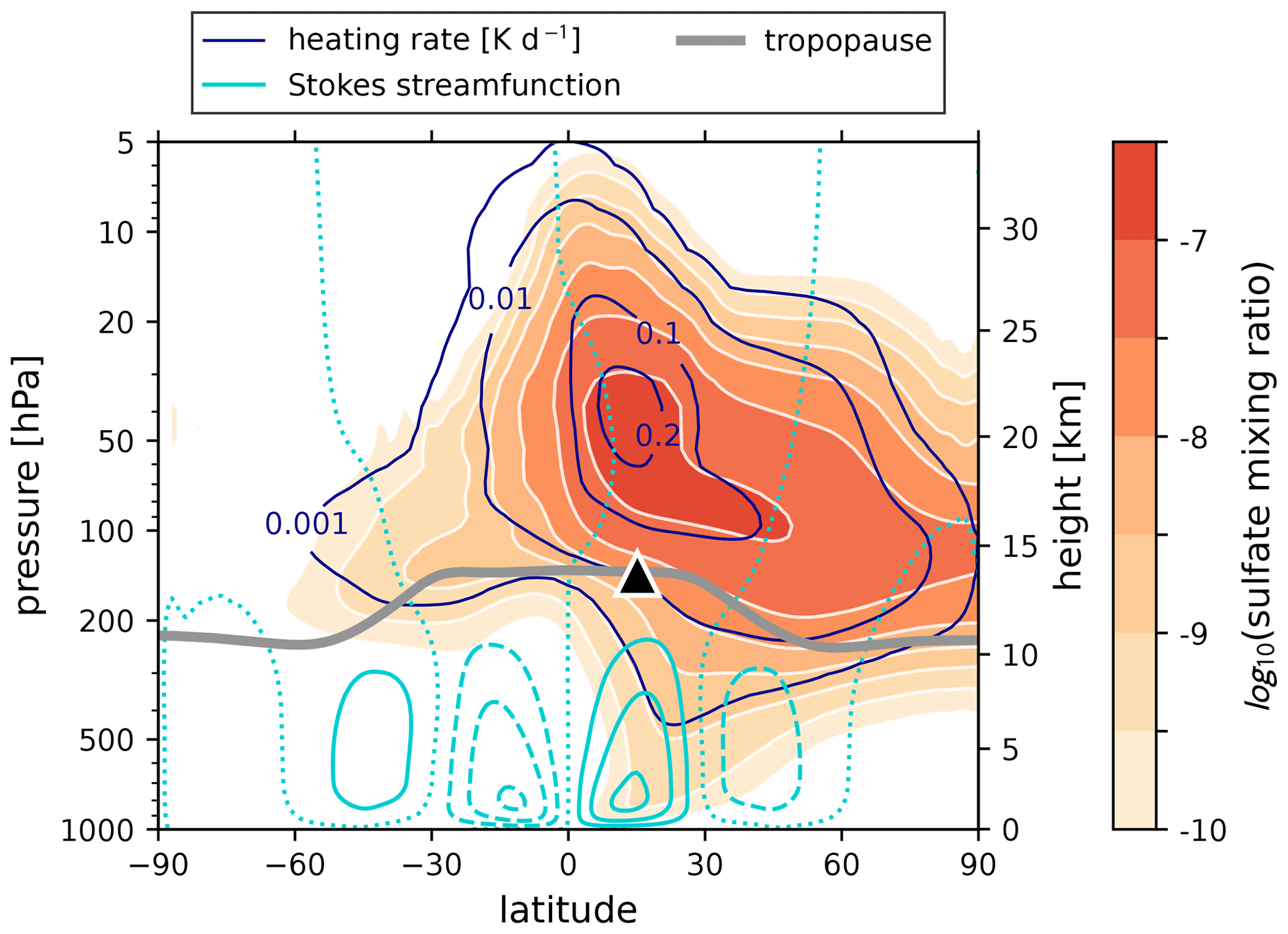
Figure 9 The 30 d time average over days 60–90 post-injection of the logarithmic zonal-mean sulfate mixing ratio (kg tracer)(kg dry air)⁻¹. Also plotted in solid dark blue contours is the local stratospheric heating rate by longwave absorption (K d⁻¹), with logarithmic intervals between contours 0.001, 0.01, and 0.1, and a final contour drawn at 0.2. Cyan contours show the Stokes streamfunction (Eq. 41) with intervals of 3×10¹⁰ kg s⁻¹. Negative (positive) contours are dashed (solid), and the zero line is dotted. The thick gray line shows the tropopause. The height axis is obtained from the model's diagnostic geopotential height.

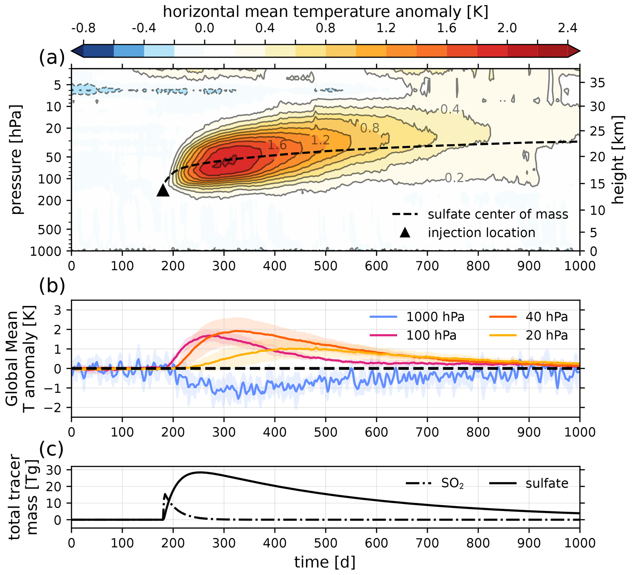
Figure 10 (a) Ensemble-mean temperature anomalies with respect to a volcanically quiescent reference period of 10 years, averaged at each model level over all longitudes and all latitudes within 20° of the injection (from 5° S to 35° N). Contour intervals are drawn every 0.2 K. The height axis is obtained from the model's diagnostic geopotential height. The black triangle shows the height of the initial mass injection distribution peak and the time of the eruption at 180 d. The dashed black line shows the center of mass of the volcanic sulfate distribution. (b) The temperature anomaly data shown in panel (a), chosen for certain pressure levels, including the surface (1000 hPa). The shading for each curve shows the standard deviation of the ensemble members. (c) The globally integrated tracer mass time series for SO₂ and sulfate.

5 Conclusions

The injection, evolution, and forcing described in this article constitute an idealized prognostic simulation of volcanic aerosol emission and impact development. Previously, it was not possible to include volcanic forcing routines in such a simple environment, as they inherently depend on a complex library of physical subgrid parameterizations. To our knowledge, there is no other option for simulating sulfur forcing with a prognostic aerosol treatment in a Held–Suarez-based atmosphere.

This idealized prognostic simulation has isolated the volcanic event from other sources of variability and established a direct relationship between forcing (SO₂ emission) and downstream (stratospheric and surface temperature anomalies) impacts. Delivering these features as a computationally affordable capability facilitates the development of new multistep data analytic techniques designed to improve downstream attribution. This simulation has been used in the development of explainable AI techniques which measure the importance of input variables for the prediction of downstream temperature (McClernon et al., 2024). In the near future, we anticipate its broader utility in developing other multistep attribution methods and in capitalizing on the development of the LV ensemble formulation to establish robust responses to a particular atmospheric state.

This work is a new addition to an idealized AGCM hierarchy that can be used to study phenomena in isolation. Examples of this model hierarchy include Sheshadri et al. (2015) and Hughes and Jablonowski (2023), who studied the effects of topography on the atmospheric flow, or Polvani and Kushner (2002) and Gerber and Polvani (2009), who assessed polar jets and hemispheric asymmetry. Other idealized configurations focus on simple moist flows with moisture feedbacks (Frierson et al., 2006; Thatcher and Jablonowski, 2016), tropical cyclones (Reed and Jablonowski, 2012), tracer-based cloud microphysics (Frazer and Ming, 2022; Ming and Held, 2018), age-of-air tracers (Gupta et al., 2020), the Madden–Julian oscillation (MacDonald and Ming, 2022), or climate change forcing (Butler et al., 2010). In addition, this work builds upon previous idealizations of volcanism using simpler prescribed forcing approaches. This includes Toohey et al. (2016), who provided a set of zonally symmetric volcanic aerosol optical properties tuned to observational data, and DallaSanta et al. (2019), who subjected a set of atmospheric models of increasing complexity to a prescribed aerosol forcing in the form of controlled solar dimming and steady, zonally uniform lower-stratospheric temperature tendencies.

We illustrated that our implementation can be used to mimic the spatiotemporal temperature anomaly signatures of large volcanic eruptions, and we presented one specific parameter tuning that gives rise to a Pinatubo-like event. Our design intentionally leaves out many details which we felt would increase physical complexity, without being necessary for producing realistic atmospheric impacts for attribution studies (e.g., gravitational settling of aerosols). Nevertheless, the formulation remains flexible for modifications. Our parameterizations can be tuned toward eruption scenarios other than the 1991 Mt. Pinatubo event. They can also could support any number of co-injected tracer species, concurrence of multiple eruptions, and injections at any latitude and height. In fact, the description is generic enough that, by replacing the vertical and/or temporal injection profiles, we could imagine simulating the aerosol direct effect of various localized emission events of the troposphere (e.g., wildfire smoke) or the stratosphere (e.g., geoengineering SAI experiments) in an idealized model configuration.

Appendix A: Modification of the Held–Suarez–Williamson forcing to accommodate higher model tops

As suggested in Sect. 2.2, we make two modifications to the implementation of the HSW forcing scheme, i.e., (1) the adjustment of the radiative equilibrium temperature T_eq near the model top and (2) the inclusion of an additional sponge-layer wind-damping mechanism, which are described in Sect. A1–A2. Figure 1a shows the radiative equilibrium temperature with our modifications together with the employed vertical profiles for the sponge-layer and surface-layer damping.

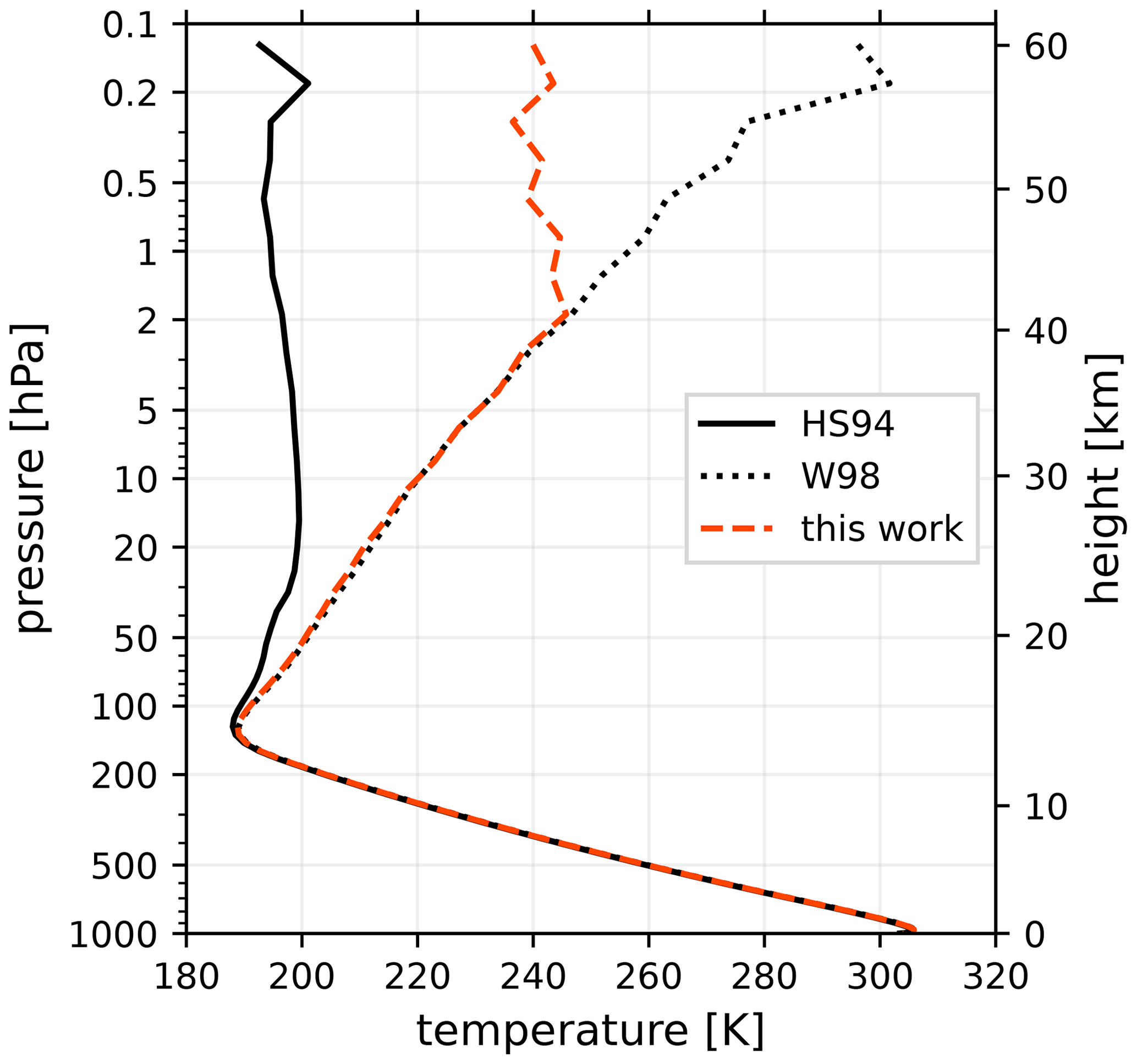
Figure A1 Zonal-mean tropical temperature profiles resulting from E3SMv2 runs of the HS94 (solid black), W98 (dotted black), and our modified HSW (dashed red) forcing schemes, averaged over −7° S to 7° N. The runs were performed at the ne16pg2 resolution for 10 years, with the first 5 years discarded as spinup and the time mean of the latter 5-year period shown here. The height axis is derived from the geopotential height of the modified HSW run, with the same averaging performed.

A1 Modified radiative equilibrium temperature

The model employed in the experiments of Williamson et al. (1998) features a top at ∼ 3 hPa, while the standard E3SMv2 model top is located at ∼ 60 km, or 0.1 hPa. Applying the temperature relaxation profile as published in Williamson et al. (1998) to E3SMv2 therefore results in undesired reversals in the polar lapse rate near 2 hPa as well as temperatures at the tropical model top at around 60 km in excess of 300 K. Observed monthly-mean zonal-mean tropical temperature peaks near 50 km are closer to ∼ 260 K (Holton and Hakim, 2013). We experimented with modifying the lapse rate parameters in the HSW T_eq as suggested by Williamson et al. (1998) and implemented by Yao and Jablonowski (2016), but ultimately we chose to attempt to retain more realistic temperatures of the upper stratosphere by simply imposing a lapse rate of zero for p<2 hPa in T_eq. Specifically, the equilibrium temperature used in our modified HSW forcing is

$$\begin{array}{}\text{(A1)}& T_{\text{eq}}(\mathit{\varphi },p)=T_{\text{eq,HSW}}(\mathit{\varphi },\text{max}\left(p,p^{*}\right)),\end{array}$$

where T_eq,HSW(ϕ,p) is the form presented in Appendix A of Williamson et al. (1998), and $p^{*}=\mathrm{2}$ hPa.

Other than this modification, the design and parameter choices of T_eq are identical to those defined in Held and Suarez (1994) and Williamson et al. (1998). From Williamson et al. (1998), we inherit the property that the original implementation of Held and Suarez (1994) applies below 100 hPa. Figure A1 shows zonally averaged tropical temperature profiles resulting from 5-year E3SMv2 runs responding to the specifications of Held and Suarez (1994), Williamson et al. (1998), and our modified HSW forcings. The three implementations exhibit no difference in tropopause structure. Above the tropopause, the HS model approaches a constant temperature near 200 K, while W98 and the modified HSW forcings share a lapse rate of approximately 2.6 K km⁻¹ until 2 hPa, where they diverge.

A2 Sponge-layer Rayleigh damping

Following Held and Suarez (1994) and Williamson et al. (1998), we use the inverse timescales k_v(p) and k_T(ϕ,p) for Rayleigh damping of the velocity v and relaxation temperature T toward T_eq, respectively. In addition, we add a second Rayleigh damping mechanism in the sponge layer (so-called since it acts to absorb vertically propagating waves near the model top). The vertical profile that we choose for the damping strength follows the implementation of Harris et al. (2021) (their Eq. 8.15), with a monotonic onset from ∼ 100 Pa to the model top:

$$\begin{array}{}\text{(A2)}& k_s\left(p\right)=k_{\mathrm{0}}\text{sin}{\left({\displaystyle \frac{\mathit{\pi }}{\mathrm{2}}}{\displaystyle \frac{\text{log}({\mathit{\eta }}_c/\mathit{\eta })}{\text{log}({\mathit{\eta }}_c/{\mathit{\eta }}_T)}}\right)}^{\mathrm{2}}.\end{array}$$

Here, the normalized pressure coordinate is $\mathit{\eta }\equiv p/p_{\mathrm{0}}$, with p₀=1000 hPa. We define the onset position at ${\mathit{\eta }}_c=\left(\mathrm{1}\mathrm{hPa}\right)/p_{\mathrm{0}}$ and the normalized pressure at the model top as ${\mathit{\eta }}_T\equiv p_{\text{top}}/p_{\mathrm{0}}$. The maximum strength of the damping is set using $k_{\mathrm{0}}=\mathrm{1}/$ (3 d).

Given these modifications, the wind and temperature tendencies will be updated at each physics time step by

$$\begin{array}{}\text{(A3)}& {\displaystyle \frac{\partial T}{\partial t}}=-k_T(\mathit{\varphi },p)\left(T-T_{\text{eq}}\right),\text{(A4)}& {\displaystyle \frac{\partial \mathit{v}}{\partial t}}=\left(-k_s\left(p\right)-k_v\left(p\right)\right)\mathit{v},\end{array}$$

which form the totality of the parameterized forcings in our model (in the absence of volcanic injections). The vertical profile of the total wind damping (k_s(p)+k_v(p)) is shown in Fig. 1a.

Appendix B: Residual circulation of the modified Held–Suarez–Williamson atmosphere

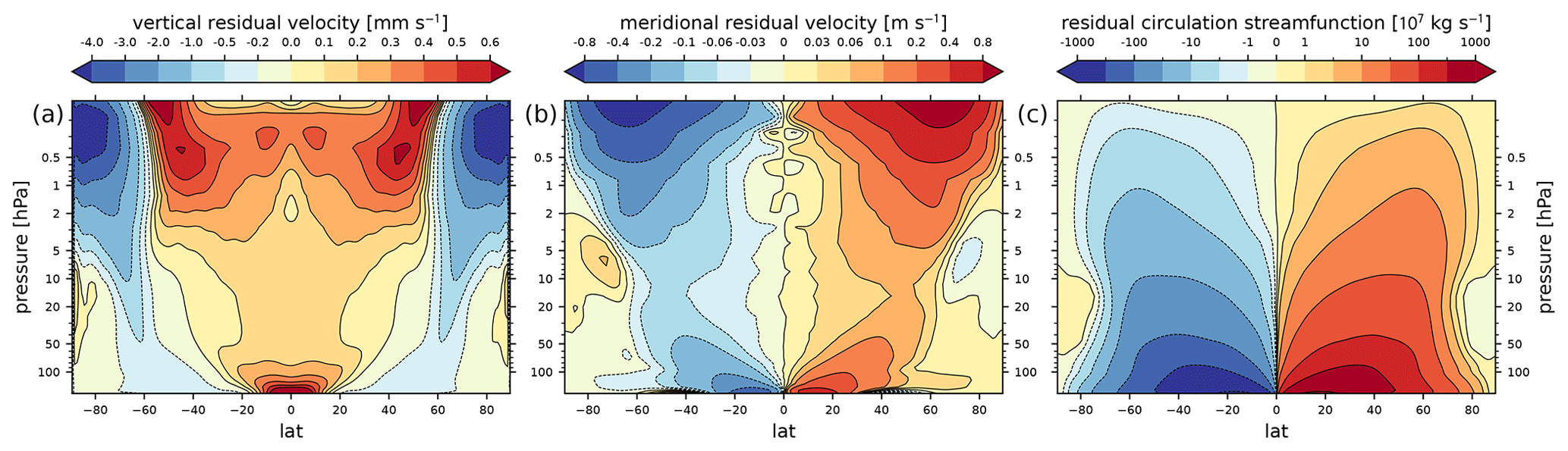
Figure B1 Stratospheric residual circulation of the HSW atmosphere averaged over 5 years, after a 5-year spinup period. The vertical scale extends from 100 hPa to the model top near 0.1 hPa. (a) The vertical residual velocity (mm s⁻¹). Contours are irregularly spaced. (b) The meridional residual velocity (m s⁻¹). Contours are irregularly spaced. (c) The residual streamfunction (10⁷ kg s⁻¹). Contours unlabeled on the color bar are 3 times their neighboring contour toward zero. That is, the positive contours are $\mathrm{1},\mathrm{3},\mathrm{10},\mathrm{30},\mathrm{100},\mathrm{\dots }$

A discussion of the residual circulation of the HSW atmosphere was presented in Sect. 4.2. Figure B1 shows the vertical and meridional components of the residual velocity in the meridional plane from 100 to 0.1 hPa averaged over 5 years of integration of a HSW run with no volcanic injections, after a 5-year spinup period. Also shown is the residual circulation mass streamfunction. The meridional residual velocity, vertical residual velocity, and residual velocity streamfunction are exactly the forms presented as Eqs. (A6), (A7), and (A8), respectively, of Gerber and Manzini (2016).

The residual vertical and meridional velocities agree qualitatively well with those computed from springtime averages of reanalysis data as presented in Fujiwara et al. (2022) (their Figs. 11.12 and 11.15). Curious features of the HSW residual velocities are the sign reversals in both residual velocity components as well as the streamfunction in the polar stratosphere near 10–30 hPa. These features appear in some, but not all, of the springtime reanalysis results of Fujiwara et al. (2022) in the meridional residual velocity, though not in the vertical residual velocity.

Appendix C: Recommendations for model parameter tuning

This section provides recommendations for retuning the idealized volcanic forcing model presented in this work. This information may be useful if the parameterizations are to be activated with a different dynamical core resolution or if the model parameters are altered to represent a different aerosol injection scenario. The results shown in Sect. 4.2 only represent the Pinatubo-like parameter configuration given in Table 1 for a grid of nominal 200 km horizontal spacing (the ne16pg2 grid).

In our original implementation, the parameter tuning was done by manually perturbing parameter values after a preliminary estimate, running simulations, and observing the results of certain target metrics. In practice, the tuning process is an iterative one, since changing the extinction coefficients changes the local aerosol heating rates, which in turn changes the local circulation and thus the plume transport. Achieving a plume that leads to both a realistic stratospheric distribution and global-mean temperature anomalies was the goal.

Each subsection below describes the tuning of a certain effect, first listing the relevant parameters, the target metric used, and the method of the initial estimate. We suggest that future tuning efforts of our parameterizations follow these procedures. In what follows, we refer to a “passive” run as one where the tracer injection and sulfate production occur as described in Sect. 3.1–3.2 but all radiative feedback is disabled and the tracers are only transported.

C1 SW mass extinction coefficients

Parameters:	bSW,ash, $b_{\mathrm{SW},{\mathrm{SO}}_{\mathrm{2}}}$, bSW,sulfate
Target metric:	maximum zonal-mean AOD
Initial estimate method:	passive simulation runs

In tuning the shortwave extinction coefficients, we can make a preliminary constraint of b_SW, such that the resulting AOD τ_i is representative of post-Pinatubo observations. Zonal-mean AODs observed in the months and years following the Pinatubo eruption peaked near 0.2–0.5 (Dutton and Christy, 1992; Stenchikov et al., 1998; Mills et al., 2016), and passive runs of our injection protocol yield maximum zonal-mean column mass burdens (as a sum of all species) which peak near 2×10⁷ kg approximately 3 weeks post-injection near the Equator. Constraining columns of this mass burden to have an AOD of 0.35, Eq. (23) then suggests

$$\begin{array}{}\text{(C1)}& \begin{array}{rl}{\mathit{\tau }}_i=\mathrm{0.35}& =b_{\text{SW}}{\displaystyle \frac{M_i}{a_i}}\\ & \Rightarrow b_{\text{SW}}={\displaystyle \frac{\mathrm{0.35}{a}_i}{\mathrm{2}\times {\mathrm{10}}^{\mathrm{7}}\mathrm{kg}}}=\mathrm{700}{\displaystyle \frac{{\text{m}}^{\mathrm{2}}}{\text{kg}}},\end{array}\end{array}$$

where we took $a_i=(\mathrm{200}\times \mathrm{200})$ km², consistent with a ∼ 2° resolution near the Equator. Starting with this initial estimate, we then manually and iteratively altered the b_SW parameters until converging upon the desired peak zonal-mean AOD (see Fig. 8), with the final parameter values given in Table 1. These final values are an acceptable starting estimate for new tuning efforts. Since Eq. (C1) involves a factor of (area) / (mass), the b_SW parameters should be, in principle, independent of resolution. However, higher resolutions could resolve finer, higher-density structures in the tracer fields and might therefore be indirectly dependent on the grid spacing.

C2 Surface heat transfer efficiency

Parameter:	ζ
Target metric:	minimum mean surface
	temperature anomaly
Initial estimate method:	derived constraint
	from the literature

As we do not know a priori the relationship between surface cooling rates and the realized surface temperature anomaly in the HSW atmosphere, we make a preliminary tuning of ζ, assuming a known maximum negative cooling rate. In their model experiments of the Pinatubo initial plume dispersion, Stenchikov et al. (2021) observed that spatial-mean values of the surface cooling in the equatorial belt from 0 to 15° N post-injection are around $\mathrm{\Delta }T=-\mathrm{0.02}$ K d⁻¹ (their Fig. 6), which is also qualitatively consistent with Stenchikov et al. (1998) and Ramachandran et al. (2000). In this region, we have already roughly constrained τ to be near 0.35 in Eq. (C1). Solving Eq. (35) for ζ in this case gives

$$\begin{array}{}\text{(C2)}& \begin{array}{rl}\left(-\mathrm{0.02}{\displaystyle \frac{\text{K}}{\text{d}}}\right)& =\mathit{\zeta }{\displaystyle \frac{\mathrm{1}}{c_p}}{\displaystyle \frac{a_i}{m_{i,\text{surf}}}}{\displaystyle \frac{\left(\mathrm{1}\text{d}\right)}{\left(\mathrm{86400}\text{s}\right)}}{I}_{\text{SW}}\\ & \left(\exp (-\mathrm{0.35})-\mathrm{1}\right)\\ & \Rightarrow {\mathit{\zeta }}^{-\mathrm{1}}={\displaystyle \frac{\mathrm{1}}{c_p}}{\displaystyle \frac{a_i}{m_{i,\text{surf}}}}{\displaystyle \frac{\left(\mathrm{1}\text{d}\right)}{\left(\mathrm{86400}\text{s}\right)}}\\ & {\displaystyle \frac{\mathrm{1}}{\left(-\mathrm{0.02}\frac{\text{K}}{\text{d}}\right)}}{I}_{\text{SW}}\left(\exp (-\mathrm{0.35})-\mathrm{1}\right).\end{array}\end{array}$$

Using I_SW from Eq. (5) at latitude ϕ=0 and $m_{i,\text{surf}}=(\mathrm{\Delta }{p}_{i,k}{a}_i/g)$ with $\mathrm{\Delta }{p}_{i,k}=\mathrm{10}$ hPa (corresponding to ∼100 m or κ=2 for Eq. (37) in E3SMv2), this gives

$$\begin{array}{}\text{(C3)}& \mathit{\zeta }\approx \mathrm{1.5}\times {\mathrm{10}}^{-\mathrm{3}},\end{array}$$

which is independent of horizontal resolution, since a_i cancels in Eq. (C2) (though it is dependent on vertical resolution). The tuned value of $\mathrm{4.0}\times {\mathrm{10}}^{-\mathrm{3}}$ is several times larger than this estimate, since we ultimately required average tropical cooling rates significantly lower than −0.02 K d⁻¹ (see Fig. 8a) to obtain a significant surface-level temperature anomaly near −1 K. This requirement may simply be due to the strength of the HSW temperature relaxation at the lowest model levels needing a stronger forcing to overcome.

C3 LW mass extinction coefficients

Parameters:	bLW,ash, $b_{\mathrm{LW},{\mathrm{SO}}_{\mathrm{2}}}$, bLW,sulfate
Target metrics:	maximum mean stratospheric
	temperature anomaly and
	lofted sulfate plume height
Initial estimate methods:	passive simulation run and
	the derived constraint from the
	literature

In making an initial estimate of the LW mass extinction parameters, we first simplify Eq. (28) to an approximate form where the aerosol radiative shadowing effect is not allowed (assuming I_LW is incident on all vertical positions of the column):

$$\begin{array}{}\text{(C4)}& \mathrm{\Delta }{I}_{i,k}=I_{\text{LW}}\left[\mathrm{1}-\text{exp}\left(-b_{\text{LW}}{\displaystyle \frac{q_{i,k}\mathrm{\Delta }{p}_{i,k}}{g}}\right)\right].\end{array}$$

This simplified attenuation implies a stratospheric heating rate in the form of Eq. (30) of

$$\begin{array}{}\text{(C5)}& \begin{array}{rl}\mathrm{\Delta }{T}_{i,k}& ={\displaystyle \frac{\mathrm{1}}{c_p}}{\displaystyle \frac{a_i}{m_{i,k}}}{I}_{\text{LW}}\left[\mathrm{1}-\text{exp}\left(-b_{\text{LW}}{\displaystyle \frac{q_{i,k}\mathrm{\Delta }{p}_{i,k}}{g}}\right)\right]\\ & \approx -{\displaystyle \frac{\mathrm{1}}{c_p}}{\displaystyle \frac{a_i}{m_{i,k}}}{I}_{\text{LW}}{b}_{\text{LW}}{\displaystyle \frac{q_{i,k}\mathrm{\Delta }{p}_{i,k}}{g}},\end{array}\end{array}$$

where the approximation $e^x\approx (\mathrm{1}+x)$ was used. From observations by previous modeling studies (Stenchikov et al., 2021; Ramachandran et al., 2000; Stenchikov et al., 1998), we expect monthly-mean zonal-mean values for the stratospheric heating rate during month 3 post-injection to approach ΔT=0.3 K d⁻¹ in the tropics. Note that, in the works cited for this figure, this is the total heating rate due to contributions of visible, near-infrared, and infrared radiation. In this work, though we refer to this heating effect specifically as “longwave”, we are tuning to the total heating rate of 0.3 K d⁻¹.

The estimate of b_LW can now proceed analogously to Sect. C1–C2 by inverting Eq. (C5) for b_LW. Passive runs of our injection protocol yield sulfate monthly-mean zonal-mean mixing ratios at this time and locations of about 10⁻⁶ kg kg⁻¹. The preliminary b_LW estimate is then

$$\begin{array}{}\text{(C6)}& \Rightarrow b_{\text{LW}}={\displaystyle \frac{\left(\mathrm{0.3}\frac{\text{K}}{\text{d}}\right)}{\left({\mathrm{10}}^{-\mathrm{6}}\frac{\text{kg}}{\text{kg}}\right)}}{\displaystyle \frac{g{c}_p{m}_{i,k}}{a_i{I}_{\text{LW}}\mathrm{\Delta }{p}_{i,k}}}{\displaystyle \frac{\left(\mathrm{1}\text{d}\right)}{\left(\mathrm{86400}\text{s}\right)}}{\displaystyle \frac{{\text{m}}^{\mathrm{2}}}{\text{kg}}}.\end{array}$$

Evaluating this form with I_LW(ϕ=0) from Eq. (4) and using $m_{i,\text{surf}}=(\mathrm{\Delta }{p}_{i,k}{a}_i/g)$ gives

$$\begin{array}{}\text{(C7)}& b_{\text{LW}}\approx \mathrm{6.2}{\displaystyle \frac{{\text{m}}^{\mathrm{2}}}{\text{kg}}}.\end{array}$$

Comparing this estimate with Eq. (C1), our formulation implies that the aerosols are much more efficient at attenuating shortwave radiation (by scattering) than longwave radiation (by absorption).

From this estimate, we then manually and iteratively adjust the three b_LW parameters for ash, SO₂, and sulfate. As suggested in Sect. 3.5, this tuning is done with two target metrics in mind: (1) b_{LW, sulfate} is tuned to give rise to maximum stratospheric temperature anomalies of 2–3 K, and (2) b_{LW, ash} is tuned to control the initial lofting of the fresh, dense plume, such that the aged sulfate population converges upon the 20–30 km vertical layer. The parameter $b_{\mathrm{LW},{\mathrm{SO}}_{\mathrm{2}}}$ contributes to both the initial lofting and the short-term temperature anomalies. Thus, the final tuned parameters (given in Table 1) arrive at very different values.

C4 Avoiding a low injection height by revising the LW mass extinction coefficient tuning

As alluded to in Sect. 3.5 and Appendix C3, there is some degeneracy between b_LW,ash and $b_{\mathrm{LW},{\mathrm{SO}}_{\mathrm{2}}}$ for controlling the initial heating of the aerosol plume as well as degeneracy between b_LW,sulfate and $b_{\mathrm{LW},{\mathrm{SO}}_{\mathrm{2}}}$ for controlling the stratospheric temperature anomalies during the first few months post-injection. This makes the manual process of iteratively tuning the parameters more laborious. In the present case, it also results in the implementation of an unusually low initial injection height of μ=14 km. Specifically, we did not tune $b_{\mathrm{LW},{\mathrm{SO}}_{\mathrm{2}}}$ along with b_LW,ash and instead needed to compensate for the aggressive early plume lofting by lowering μ.

The tuning process would be easier, and a higher initial injection height of 18–20 km could be more easily supported, if the degeneracy between these three extinction parameters were removed. We suggest having the SO₂ tracer behave instead as a radiatively passive tracer, acting only as the vehicle for sulfate production, by setting $b_{\mathrm{LW},{\mathrm{SO}}_{\mathrm{2}}}=\mathrm{0}$ and $b_{\mathrm{SW},{\mathrm{SO}}_{\mathrm{2}}}=\mathrm{0}$. In this case, the LW mass extinction coefficients for ash and sulfate would be independent knobs for the lofting height and long-term temperature anomalies, respectively. We would consider this tuning choice an improvement of the parameterization.