Implementation and assessment of a model including mixotrophs and the carbonate cycle (Eco3M_MIX-CarbOx v1.0) in a highly dynamic Mediterranean coastal environment (Bay of Marseille, France) – Part 2: Towards a better representation of total alkalinity when modeling the carbonate system and air–sea CO₂ fluxes

The Bay of Marseille (BoM), located in the northwestern Mediterranean Sea, is affected by various hydrodynamic processes (e.g., Rhône River intrusion and upwelling events) that result in a highly complex local carbonate system. In any complex environment, the use of models is advantageous since it allows us to identify the different environmental forcings, thereby facilitating a better understanding. By combining approaches from two biogeochemical ocean models and improving the formulation of total alkalinity, we develop a more realistic representation of the carbonate system variables at high temporal resolution, which enables us to study air–sea CO₂ fluxes and seawater pCO₂ variations more reliably. We apply this new formulation to two particular scenarios that are typical for the BoM: (i) summer upwelling and (ii) Rhône River intrusion events. In both scenarios, our model was able to correctly reproduce the observed patterns of pCO₂ variability. Summer upwelling events are typically associated with a pCO₂ decrease that mainly results from decreasing near-surface temperatures. Furthermore, Rhône River intrusion events are typically associated with a pCO₂ decrease, although, in this case, the pCO₂ decrease results from a decrease in salinity and an overall increase in total alkalinity. While we were able to correctly represent the daily range of air–sea CO₂ fluxes, the present configuration of Eco3M_MIX-CarbOx does not allow us to correctly reproduce the annual cycle of air–sea CO₂ fluxes observed in the area. This pattern directly impacts our estimates of the overall yearly air–sea CO₂ flux as, even if the model clearly identifies the bay as a CO₂ sink, its magnitude was underestimated, which may be an indication of the limitations inherent in dimensionless models for representing air–sea CO₂ fluxes.

1 Introduction

Since the industrial revolution, atmospheric CO₂ concentrations have been constantly increasing (Mauna Loa Observatory: https://gml.noaa.gov/ccgg/trends/, last access: 20 June 2024). By absorbing large amounts of CO₂, the global ocean acts as an important sink of anthropogenic CO₂. Recent estimates suggest that this absorption corresponds to roughly 25 % of annual emissions (Friedlingstein et al., 2022). During this absorption process, CO₂ undergoes a series of acid–base reactions that eventually lead to the formation of carbonate ions (CO${}_{\mathrm{3}}^{\mathrm{2}-}$). Initially, dissolved CO₂ reacts with water to form carbonic acid (H₂CO₃), which then dissociates into bicarbonate (HCO${}_{\mathrm{3}}^{-}$) and hydronium (H⁺) ions. In turn, HCO${}_{\mathrm{3}}^{-}$ dissociates into CO${}_{\mathrm{3}}^{\mathrm{2}-}$ and H⁺ ions. Increased uptake of atmospheric CO₂ modifies this acid–base reaction chain, thus affecting the associated species concentrations, particularly of H⁺ ions, which increase significantly, resulting in a decrease in seawater pH. This phenomenon, known as ocean acidification (OA), is ubiquitous, as confirmed through global observations (Feely et al., 2009; Dore et al., 2009; Gonzales-Dávila et al., 2010; Bates et al., 2012). The increased uptake of atmospheric CO₂ not only results in lower pH but also modifies the overall carbonate equilibrium, which is slowly shifting towards higher HCO${}_{\mathrm{3}}^{-}$ and H₂CO₃ concentrations and lower CO${}_{\mathrm{3}}^{\mathrm{2}-}$ concentrations, which makes it more difficult for marine calcifiers to form their calcium carbonate shells (Orr et al., 2005).

Coastal oceans (depth <200 m, Gattuso et al., 1998) account for over 10 % (0.18 to 0.45 Pg C per year; Laruelle et al., 2010, 2014) of the total oceanic CO₂ uptake (Thomas et al., 2004) and are therefore particularly impacted by OA, generally exhibiting more pronounced localized decreases in pH (e.g., Kapsenberg et al., 2017; Luchetta et al., 2010). Nonetheless, coastal environments are highly complex, mainly due to their high spatial and temporal variability, which makes their response to changes difficult to predict (Carstensen et al., 2018). Their proximity to the land means they are particularly exposed to anthropogenic pressures (run off and riverine input of anthropogenic nutrients and other chemical products, as well as organic matter rejects). Moreover, they are affected by strong physical forcings (e.g., tides, salinity gradients, wind-induced currents) and account for about 30 % of all oceanic primary production, which typically results in rich and diverse ecosystems (Gattuso et al., 1998).

The Mediterranean Sea is comparatively small and semi-enclosed; it receives nutrients through several pathways including Saharan dust depositions (Guerzoni et al., 1997) and numerous riverine inputs (e.g., Hopkins, 1992; Salat et al., 2002; Pujo-Pay et al., 2006). Considering the fact that the Mediterranean Sea is mostly oligotrophic (Morel and André, 1991), these inputs are highly significant for phytoplankton growth (Revelante and Gillmartin, 1976; Ludwig et al., 2009). These features render the biogeochemistry of the Mediterranean Sea particularly complex, especially with regard to the carbonate system. Several studies have investigated the carbonate system and air–sea CO₂ fluxes in these areas, typically using point measurements from various locations, including the Ligurian Sea (De Carlo et al., 2013; Kapsenberg et al., 2017), the Bay of Marseille (BoM; Wimart-Rousseau et al., 2020a), the Gulf of Trieste (Ingrosso et al., 2016), and the Adriatic Sea (Urbini et al., 2020). Overall, these studies agree with findings by Roobaert et al. (2019), who showed that coastal systems mostly act like CO₂ sinks on a yearly basis, although the CO₂ uptake shows a significant intra-annual variability.

Most modeling approaches to investigate carbonate system variables typically employ 3D coupled physical–biogeochemical models and focus on larger coastal areas (e.g., Artioli et al., 2014; Bourgeois et al., 2016). If the focus is on smaller areas, this requires higher spatial and temporal resolutions to correctly represent the relevant processes (Bourgeois et al., 2016). However, higher spatial and temporal resolutions often result in a significant increase in the calculation time, which makes the repetition of numerical experiments – an important step to better understand the global functioning of the area and its reaction to environmental forcings – more difficult. A solution to avoid important calculation times is to use a dimensionless model. This type of model allows us to conduct large numbers of tests in short amounts of time. For instance, Lajaunie-Salla et al. (2021) used the dimensionless Eco3M-CarbOx model, which contains a carbonate module in which a carbonate system is resolved by using total alkalinity (TA) and dissolved inorganic carbon (DIC). Even if the DIC, the oceanic partial pressure of CO₂ (pCO₂), and the total pH (pH_T) representations look reliable, Eco3M-CarbOx tends to minimize the range of TA variations during the year, resulting in a near-constant TA (Lajaunie-Salla et al., 2021).

Here, we try to provide a more realistic representation of carbonate system variables in the BoM. As a starting point, we used the concept of the dimensionless Eco3M-CarbOx model (Lajaunie-Salla et al., 2021), which aims to represent a small volume of surface water (i.e., 1 m³) in the BoM. We developed a planktonic ecosystem model which contains, among other things, mixotrophic organisms; modified the carbonate module described by Lajaunie-Salla et al. (2021); and added it to our newly developed planktonic ecosystem model to obtain the Eco3M_MIX-CarbOx model (v1.0). We implemented two types of TA formulations and compared the simulation results to in situ observations to identify which formulation was capable of delivering the more realistic results: (i) a formulation that only considers biological processes (referred to as autochthonous formulation) and (ii) a new TA formulation that depends only on salinity (referred to as allochthonous formulation). Furthermore, we simulate air–sea CO₂ fluxes to determine whether the BoM acts as a sink or a source of CO₂, and we provide a detailed analysis of drivers of seawater pCO₂ variations for two specific hydrodynamic processes that are typical for the BoM: (i) Rhône River intrusion and (ii) summer upwelling events. With this study, we aim to provide a new tool which will allow us to obtain a reliable representation of the carbonate system in the simplest way possible: by using a dimensionless configuration which is easy to use and adapt and which gives results in a short amount of time.

The Eco3M_MIX-CarbOx model contains both a mixotrophy compartment and a representation of the carbonate system. The model description is split into two parts: (i) a description of how the organisms and their dynamics are represented in the model, with a particular focus on mixotrophic organisms, and (ii) a more detailed description of the carbonate module and the associated dynamics. While (ii) is presented here, (i) has been presented in a companion paper (Barré et al., 2023).

2 Materials and methods

2.1 Study area

The BoM is located in the NW Mediterranean Sea, in the eastern part of the Gulf of Lion near Marseille. Due to its proximity to Marseille, the second biggest city in France, and to other urbanized areas along the coast (e.g., Fos-sur-Mer and Berre Lagoon to the west), the BoM is strongly affected by anthropogenic forcings, which results in significant inputs of anthropogenic nutrients such as ammonium (NH${}_{\mathrm{4}}^{+}$) and phosphate (PO${}_{\mathrm{4}}^{\mathrm{3}-}$), chemical products, and organic matter (OM) (Millet et al., 2018) through urban rivers. Significant quantities of nutrients and freshwater are also provided by the Rhône River (Pont et al., 2002), the delta of which is located 35 km to the west of the bay. In specific wind conditions, the Rhône River plume can be pushed eastwards, supplying the bay with nitrate, which tends to boost the productivity of the area (Gatti et al., 2006; Fraysse et al., 2013, 2014). In addition to these inputs, the biogeochemical functioning of the BoM is affected by various hydrodynamic processes including strong mistral events (Yohia, 2017); upwelling events (Millot, 1990) which generally take place in specific locations, such as the Calanques of Marseille and the Côte Bleue; development of eddies (Schaeffer et al., 2011); and intrusions of oligotrophic water masses via the Northern Current (Barrier et al., 2016; Ross et al., 2016).

In Eco3M_MIX-CarbOx, environmental forcings are provided by in situ measurements of sea surface temperature (referred to as temperature in the following), salinity, and atmospheric pCO₂ in combination with simulation data of wind speed and solar irradiance.

To evaluate our representation of carbonate system variables, we compared our model results to in situ measurements by using a carbonate parameter dataset which includes TA, DIC, and salinity data (https://www.seanoe.org, last access: 14 February 2023). Measurements are performed fortnightly at SOLEMIO station. pH_T and pCO₂ are calculated based on measured TA and DIC using CO2SYSv3 (Sharp et al., 2020, originally developed by Lewis and Wallas, 1998) on MATLAB.

A detailed description of the forcings used by the model and a map of the study area showing the location of stations where measurements were carried out, along with places of interests, can be found in Sect. 2.1 of Barré et al. (2023) (Table 1 and Fig. 1, respectively).

Table 1 Summary of simulation properties. Simulation with constant TA is detailed in the Supplement.

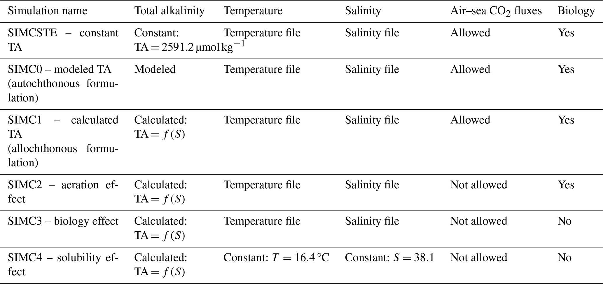
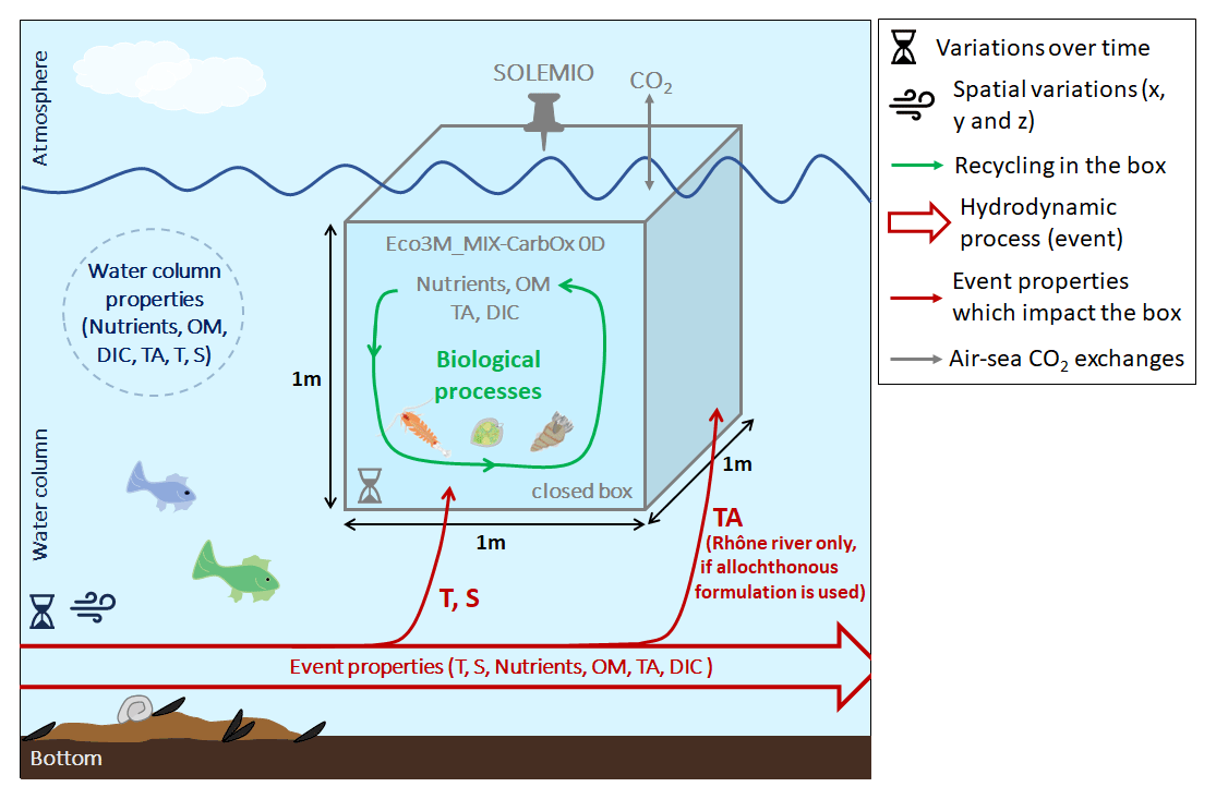
Figure 1 Schematic representation of 0D concept used in this study with Eco3M_MIX-CarbOx. T: temperature, S: salinity, and OM: organic matter.

2.2 Model description

In this study, we used the Eco3M_MIX-CarbOx model (v1.0), which was developed to represent the dynamics of the seawater carbonate system and mixotrophs in the BoM and was implemented using the Eco3M (Ecological Mechanistic and Molecular Modelling) platform (Baklouti et al., 2006a, b). Eco3M_MIX-CarbOx is a dimensionless model (0D): we consider a volume of 1 m³ of surface water at SOLEMIO station; in this volume, the state variables only vary over time as the model is not coupled with a hydrodynamic model. We chose to use a 0D configuration as this configuration has several advantages. Specifically, calculation times are low (around 45 min in our case), which allows us to make several test simulations to better understand the biogeochemical functioning of the BoM and its possible reactions to environmental forcings.

The Eco3M_MIX-CarbOx model includes seven compartments, namely zooplankton, mixotrophs, phytoplankton, heterotrophic bacteria, labile dissolved organic matter, detritic particulate organic matter, and dissolved inorganic matter, with the following carbonate system variables: dissolved inorganic carbon (DIC), total alkalinity (TA), pH calculated on the total scale (pH_T), and oceanic partial pressure of CO₂ (pCO₂). The carbonate system resolution required knowledge of at least two out of the four main variables of TA, DIC, pH_T, and pCO₂. As TA and DIC are conserved, a requirement for solving the source–sink state equations, the carbonate system resolution is based on those two variables in Eco3M_MIX-CarbOx. To provide a more realistic representation of the carbonate system, we modified the carbonate module described by Lajaunie-Salla et al. (2021) by focusing mainly on the state equations of TA and DIC as a realistic implementation of TA and DIC state variables is crucial to obtain reliable estimates of the diagnostic variables of pH_T and pCO₂. In addition to a modified carbonate module, Eco3M_MIX-CarbOx contains a mixotroph compartment, which is crucial for a reliable representation of TA and DIC as the presence of mixotrophs affects total photosynthesis, total respiration, and uptake and precipitation fluxes (Mitra et al., 2014).

By using the dimensionless model Eco3M_MIX-CarbOx, we aim to represent a small volume of surface water (1 m³) at the SOLEMIO station (Fig. 1). This small volume is closed, which means that (i) it does not exchange matter (i.e., nutrients, organic matter, organisms) with the water column; (ii) in our case, as we implemented a carbonate module which allows the representation of air–sea CO₂ fluxes, the only exchanges allowed between the volume and the atmosphere are the air–sea CO₂ fluxes; and (iii) within the volume, the matter is continuously recycled. As a result, when the water column is impacted by a hydrodynamic event which modifies its properties (i.e., which brings nutrients, organic matter, impact salinity, or temperature, for example), the event impacts only the temperature and salinity of the volume (note: in the volume, TA may be impacted by a specific event – for example, Rhône River intrusion in the BoM, which we detailed in Sect. 2.2.2; Fig. 1), and total N and P are supposed to be conserved within the volume as, unlike what is done for the C pool, we do not consider any external source or sink from or to the water column or the atmosphere.

In the following sections, we provide a detailed description of the carbonate system module. We also give a brief description of nutrients and organic matter representation. A detailed description of other compartments, especially of the mixotroph compartment, can be found in Barré et al. (2023). Equations and parameters used by the model are also explained in this previous study.

2.2.1 Nutrients and organic matter

As we use a dimensionless configuration, we assume that nutrients are fully the result of autochthonous biological processes. In other terms, we do not consider allochthonous inputs of nutrients (i.e., from rivers or the atmosphere, for instance; Fig. 1). For all the simulations, nutrient dynamics are represented by the following state equations:

$$\begin{array}{}\text{(1)}& \begin{array}{rl}{\displaystyle \frac{\partial {\mathrm{NO}}_{\mathrm{3}}}{\partial t}}& ={\mathrm{Nitrif}}_{{\mathrm{NO}}_{\mathrm{3}}}^{{\mathrm{NH}}_{\mathrm{4}}}-{\sum }_{i=\mathrm{1}}^{\mathrm{2}}\left({\mathrm{Upt}}_{{\mathrm{NO}}_{\mathrm{3}}}^{{\mathrm{Phy}}_{N_i}}\right)-{\mathrm{Upt}}_{{\mathrm{NO}}_{\mathrm{3}}}^{{\mathrm{CM}}_{N_i}},\\ {\displaystyle \frac{\partial {\mathrm{NH}}_{\mathrm{4}}}{\partial t}}& ={\mathrm{Excr}}_{{\mathrm{NH}}_{\mathrm{4}}}^{{\mathrm{COP}}_N}+{\mathrm{Excr}}_{{\mathrm{NH}}_{\mathrm{4}}}^{{\mathrm{NCM}}_N}+{\mathrm{Remin}}_{{\mathrm{NH}}_{\mathrm{4}}}^{{\mathrm{BAC}}_N}\\ & -{\sum }_{i=\mathrm{1}}^{\mathrm{2}}\left({\mathrm{Upt}}_{{\mathrm{NH}}_{\mathrm{4}}}^{{\mathrm{Phy}}_{N_i}}\right)-{\mathrm{Upt}}_{{\mathrm{NH}}_{\mathrm{4}}}^{{\mathrm{CM}}_N}-{\mathrm{Upt}}_{{\mathrm{NH}}_{\mathrm{4}}}^{{\mathrm{BAC}}_N}-{\mathrm{Nitrif}}_{{\mathrm{NH}}_{\mathrm{4}}}^{{\mathrm{NO}}_{\mathrm{3}}},\\ {\displaystyle \frac{\partial {\mathrm{PO}}_{\mathrm{4}}}{\partial t}}& ={\mathrm{Excr}}_{{\mathrm{PO}}_{\mathrm{4}}}^{{\mathrm{COP}}_{\mathrm{P}}}+{\mathrm{Excr}}_{{\mathrm{PO}}_{\mathrm{4}}}^{{\mathrm{NCM}}_P}+{\mathrm{Remin}}_{{\mathrm{PO}}_{\mathrm{4}}}^{{\mathrm{BAC}}_P}\\ & -{\sum }_{i=\mathrm{1}}^{\mathrm{2}}\left({\mathrm{Upt}}_{{\mathrm{PO}}_{\mathrm{4}}}^{{\mathrm{Phy}}_{P_i}}\right)-{\mathrm{Upt}}_{{\mathrm{PO}}_{\mathrm{4}}}^{{\mathrm{CM}}_P}-{\mathrm{Upt}}_{{\mathrm{PO}}_{\mathrm{4}}}^{{\mathrm{BAC}}_P},\end{array}\end{array}$$

where i represents the number of classes of organisms. The NO${}_{\mathrm{3}}^{-}$ concentration results from nitrification and phytoplankton and constitutive mixotroph (CM) uptakes. The NH${}_{\mathrm{4}}^{+}$ concentration results from copepods and non-constitutive mixotroph (NCM) excretion; remineralization by heterotrophic bacteria; uptakes by phytoplankton, CM, and heterotrophic bacteria; and losses from nitrification. The PO${}_{\mathrm{4}}^{\mathrm{3}-}$ concentration results from copepods and NCM excretion; remineralization by heterotrophic bacteria; and phytoplankton, CM, and heterotrophic bacteria uptakes.

As with nutrients dynamics, organic matter (dissolved and particulate) dynamics are only the result of autochthonous biological processes (Eqs. 2 and 3).

$$\begin{array}{}\text{(2)}& \begin{array}{rl}{\displaystyle \frac{\partial \mathrm{DOC}}{\partial t}}& ={\sum }_{i=\mathrm{1}}^{\mathrm{2}}\left({\mathrm{Exu}}_{\mathrm{DOC}}^{{\mathrm{PHY}}_{C_i}}\right)+{\sum }_{i=\mathrm{1}}^{\mathrm{2}}\left({\mathrm{Exu}}_{\mathrm{DOC}}^{{\mathrm{MIX}}_{C_i}}\right)\\ & +{\mathrm{Excr}}_{\mathrm{DOC}}^{{\mathrm{COP}}_C}+{\mathrm{Mort}}_{\mathrm{DOC}}^{{\mathrm{BAC}}_C}-{\mathrm{BP}}_{\mathrm{DOC}}^{{\mathrm{BAC}}_C}\\ {\displaystyle \frac{\partial \mathrm{DON}}{\partial t}}& ={\sum }_{i=\mathrm{1}}^{\mathrm{2}}\left({\mathrm{Exu}}_{\mathrm{DON}}^{{\mathrm{Phy}}_{N_i}}\right)+{\sum }_{i=\mathrm{1}}^{\mathrm{2}}\left({\mathrm{Exu}}_{\mathrm{DON}}^{{\mathrm{MIX}}_{N_i}}\right)\\ & +{\mathrm{Mort}}_{\mathrm{DON}}^{{\mathrm{BAC}}_N}-{\mathrm{Upt}}_{\mathrm{DON}}^{{\mathrm{CM}}_N}-{\mathrm{Upt}}_{\mathrm{DON}}^{{\mathrm{PICO}}_N}-{\mathrm{Upt}}_{\mathrm{DON}}^{{\mathrm{BAC}}_N}\\ {\displaystyle \frac{\partial \mathrm{DOP}}{\partial t}}& ={\sum }_{i=\mathrm{1}}^{\mathrm{2}}\left({\mathrm{Exu}}_{\mathrm{DOP}}^{{\mathrm{Phy}}_{P_i}}\right)+{\sum }_{i=\mathrm{1}}^{\mathrm{2}}\left({\mathrm{Exu}}_{\mathrm{DOP}}^{{\mathrm{MIX}}_{P_i}}\right)\\ & +{\mathrm{Mort}}_{\mathrm{DOP}}^{{\mathrm{BAC}}_P}-{\mathrm{Upt}}_{\mathrm{DOP}}^{{\mathrm{CM}}_P}-{\mathrm{Upt}}_{\mathrm{DOP}}^{{\mathrm{PICO}}_P}-{\mathrm{Upt}}_{\mathrm{DOP}}^{{\mathrm{BAC}}_P}\end{array}\end{array}$$

In the above, i represents the number of classes of organisms. The concentration of dissolved organic carbon (DOC), nitrogen (DON), and phosphorus (DOP) depends on phytoplankton and mixotroph exudation; copepod excretion (DOC only); heterotrophic bacteria mortality (natural mortality); and CM, PICO, and heterotrophic bacteria uptake.

$$\begin{array}{}\text{(3)}& \begin{array}{rl}{\displaystyle \frac{\partial \mathrm{POC}}{\partial t}}& =E_{\mathrm{POC}}^{{\mathrm{COP}}_C}+{\mathrm{Predation}}_{\mathrm{POC}}^{{\mathrm{COP}}_C}-{\mathrm{BP}}_{\mathrm{POC}}^{{\mathrm{BAC}}_C}\\ {\displaystyle \frac{\partial \mathrm{PON}}{\partial t}}& =E_{\mathrm{PON}}^{{\mathrm{COP}}_N}+{\mathrm{Predation}}_{\mathrm{PON}}^{{\mathrm{COP}}_N}-{\mathrm{Upt}}_{\mathrm{PON}}^{{\mathrm{BAC}}_N}\\ {\displaystyle \frac{\partial \mathrm{POP}}{\partial t}}& =E_{\mathrm{POP}}^{{\mathrm{COP}}_P}+{\mathrm{Predation}}_{\mathrm{POP}}^{{\mathrm{COP}}_P}-{\mathrm{Upt}}_{\mathrm{POP}}^{{\mathrm{BAC}}_P}\end{array}\end{array}$$

The concentration of particulate organic carbon (POC), nitrogen (PON), and phosphorus (POP) depends on copepod egestion, predation by higher trophic levels on copepods (closure terms of the model), and heterotrophic bacteria production and uptake. Particulate organic matter (POM) particles are large enough to sink; however, we do not consider a term to represent their removal from the surface box by sinking. In our case, the POM, such as with the dissolved organic matter (DOM) and nutrients, stays in the box and is constantly recycling (Fig. 1).

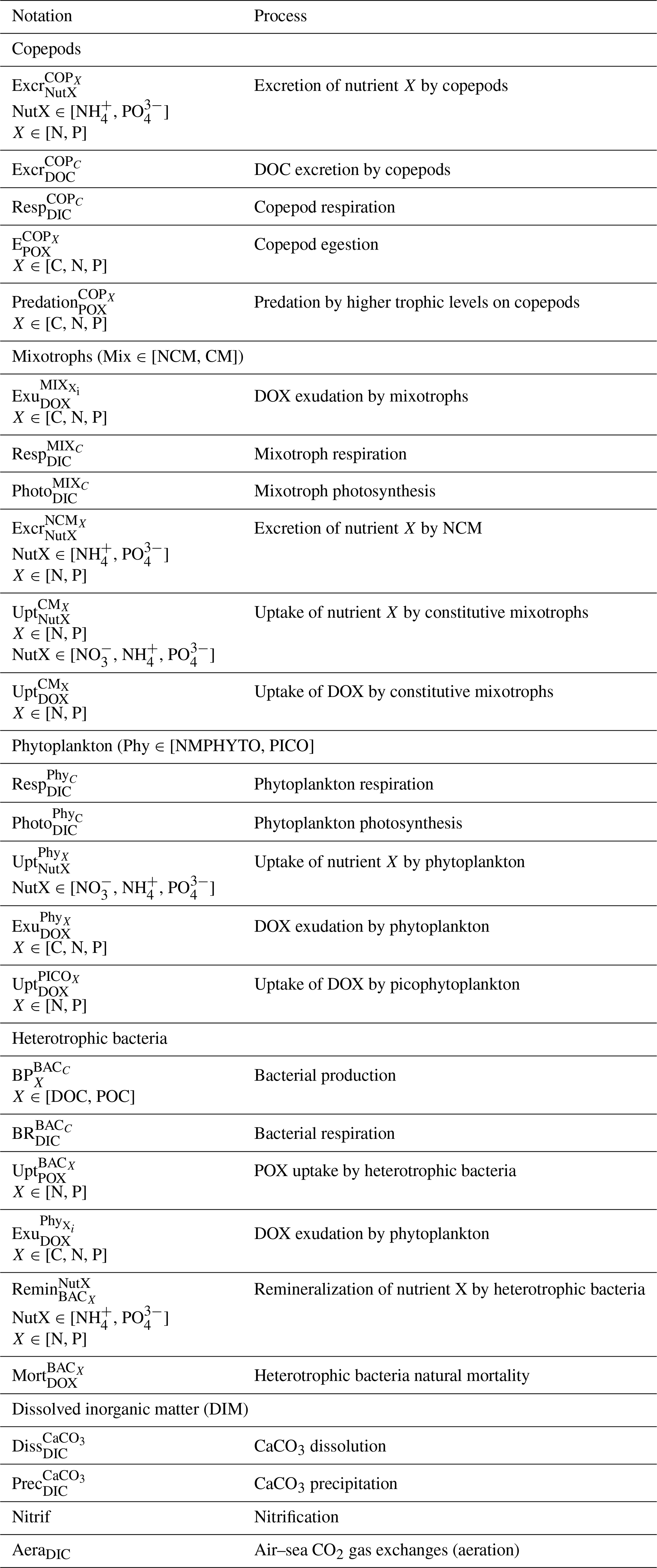
Detailed descriptions and formulations of processes can be found in Barré et al. (2023). Process notation descriptions can be found in Table A1 in Appendix A.

2.2.2 Carbonate system variable calculation

In Eco3M_MIX-CarbOx, we consider the four main carbonate system variables: TA, DIC, pH_T, and pCO₂. We describe their calculation by the model in this section.

In Eco3M-CarbOx, TA representation lacks variations during the year. Eco3M-CarbOx did not account for TA inputs by rivers, especially by the Rhône River, which has an average alkalinity of 2885 µmol kg⁻¹ (Schneider et al., 2007). To remedy this shortcoming, we decided to express TA in two ways. In the first way, we considered only autochthonous TA variations (i.e., variations in TA which result from processes which take place in the considered volume; Fig. 1). In the second way, we considered allochthonous TA variations (i.e., in the volume, TA dynamics are impacted by external contributions; Fig. 1). We then compared the outputs from each formulation to in situ data to determine which formulation delivered the more realistic results.

For the autochthonous formulation, we relied on the Eco3M-CarbOx TA state equation, which we modified to fit our modeled planktonic ecosystem. We first added a term of PO${}_{\mathrm{4}}^{\mathrm{3}-}$ remineralization by heterotrophic bacteria. We consider the fact that the uptake of 1 mol of PO${}_{\mathrm{4}}^{\mathrm{3}-}$ by phytoplankton increases TA by 1 mol and vice versa: for 1 mol of PO${}_{\mathrm{4}}^{\mathrm{3}-}$ released during remineralization, TA decreases by 1 mol (Wolf-Gladrow et al., 2007). As a last term, we included the mixotrophic uptake of nutrients. TA is calculated as follows:

$$\begin{array}{}\text{(4)}& \begin{array}{rl}{\displaystyle \frac{\partial \text{TA}}{\partial t}}& =\mathrm{2}.{\text{Diss}}_{\mathrm{TA}}^{{\mathrm{CaCO}}_{\mathrm{3}}}+{\sum }_{i=\mathrm{1}}^{\mathrm{2}}\left({\text{Upt}}_{{\mathrm{NO}}_{\mathrm{3}}}^{{\mathrm{Phy}}_{N_i}}\right)+{\text{Upt}}_{{\mathrm{NO}}_{\mathrm{3}}}^{{\mathrm{CM}}_N}\\ & +{\sum }_{i=\mathrm{1}}^{\mathrm{2}}\left({\text{Upt}}_{{\mathrm{PO}}_{\mathrm{4}}}^{{\mathrm{PHY}}_{P_i}}\right)+{\text{Upt}}_{{\mathrm{PO}}_{\mathrm{4}}}^{{\mathrm{CM}}_P}+{\text{Remin}}_{{\mathrm{NH}}_{\mathrm{4}}}^{{\mathrm{BAC}}_N}\\ & -{\sum }_{i=\mathrm{1}}^{\mathrm{2}}\left({\text{Upt}}_{{\mathrm{NH}}_{\mathrm{4}}}^{{\mathrm{PHY}}_{N_i}}\right)-{\text{Upt}}_{{\mathrm{NH}}_{\mathrm{4}}}^{{\mathrm{CM}}_N}-{\text{Remin}}_{{\mathrm{PO}}_{\mathrm{4}}}^{{\mathrm{BAC}}_P}\\ & -\mathrm{2}.{\text{Prec}}_{\mathrm{TA}}^{{\mathrm{CaCO}}_{\mathrm{3}}}-\mathrm{2}.{\text{Nitrif}}_{\mathrm{TA}},\end{array}\end{array}$$

where i represents the number of classes of organisms. Process descriptions can be found in Appendix A (Table A1), and formulations are available in Barré et al. (2023). In this formulation, TA only depends on biogeochemical processes (i.e., TA riverine inputs are excluded).

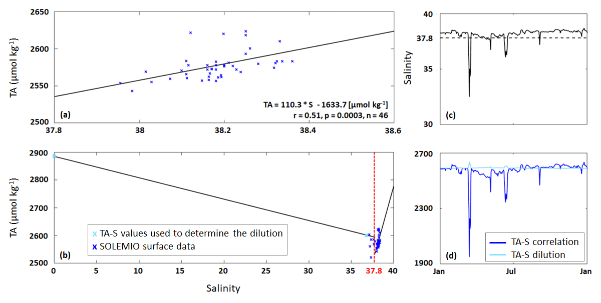
Figure 2 (a) TA–S correlation (black line) based on SOLEMIO surface data excluding low salinities ≤37.8. (b) TA–S dilution (for S≤37.8) and TA–S correlation (for S>37.8). (c) Salinity data used by the model (solid line) and S=37.8 (dashed line). (d) TA calculated from TA–S correlation (Eq. 5) and TA–S dilution (Eq. 6).

For the allochthonous formulation, we first determined an oceanic TA–S correlation (Eq. 5; Fig. 2a) using the measurements of carbonate system parameters at SOLEMIO station (see Sect. 2.1). We only considered the TA values associated with salinity values >37.8 as 37.8 was used as a threshold value to identify low-salinity events (LSEs) associated with Rhône River plume intrusions in the BoM (Fraysse et al., 2014).

$$\begin{array}{}\text{(5)}& \text{TA}=\mathrm{110.3}\cdot S-\mathrm{1633.7}\left(\mathrm{\mu }\mathrm{mol}{\mathrm{kg}}^{-\mathrm{1}}\right)\end{array}$$

Second, using only those TA values associated with LSEs, we determined a separate TA–S formulation to quantify river water dilution (Eq. 6; Fig. 2b).

$$\begin{array}{}\text{(6)}& \text{TA}=-\mathrm{7.7}\cdot S+\mathrm{2885}\left(\mathrm{\mu }\mathrm{mol}{\mathrm{kg}}^{-\mathrm{1}}\right)\end{array}$$

The carbonate dataset did not contain sufficient LSE data to create a reliable TA–S fit. Equation (6) was therefore derived based on two TA–S data pairs: TA = 2885.0 µmol kg⁻¹ and S=0, representative of water masses near the Rhône River mouth (Schneider et al., 2007), and TA = 2600.6 µmol kg⁻¹ and S=36.82, recorded at SOLEMIO station during a major LSE on 15 March 2017. Unlike Eq. (5), the TA–S dilution shows a negative slope that is typical of low-salinity river water (Fig. 2b).

We implemented both TA–S formulations in our Eco3M_MIX-CarbOx model, and the formulation to be used was chosen based on the salinity: if the salinity value used by the model for the time step considered is ≤37.8, the TA–S dilution (Eq. 6) was applied; otherwise, for a salinity value >37.8, the TA–S correlation was applied (Eq. 5, Fig. 2c, d). With this method, TA only depends on salinity (i.e., biological processes are neglected).

The DIC formulation used in our Eco3M_MIX-CarbOx model is very similar to the formulation used in Eco3M-CarbOx, except for the fact that we added the mixotrophic organisms' processes to our equation. As a result, DIC depends on phytoplankton, mixotrophs, zooplankton and bacterial respiration, air–sea CO₂ fluxes (aeration process), dissolution of CaCO₃, phytoplankton and mixotroph photosynthesis, and precipitation of CaCO₃ (Eq. 7).

$$\begin{array}{}\text{(7)}& \begin{array}{rl}{\displaystyle \frac{\partial \text{DIC}}{\partial t}}& ={\sum }_{i=\mathrm{1}}^{\mathrm{2}}\left({{\mathrm{Resp}}_{\mathrm{DIC}}}^{{\mathrm{PHY}}_{C_i}}\right)\\ & +{\sum }_{i=\mathrm{1}}^{\mathrm{2}}\left({{\mathrm{Resp}}_{\mathrm{DIC}}}^{{\mathrm{MIX}}_{C_i}}\right)+{{\mathrm{Resp}}_{\mathrm{DIC}}}^{{\mathrm{COP}}_C}\\ & +{{\mathrm{BR}}_{\mathrm{DIC}}}^{{\mathrm{BAC}}_C}+{\mathrm{Diss}}_{\mathrm{DIC}}^{{\mathrm{CaCO}}_{\mathrm{3}}}\\ & -{\sum }_{i=\mathrm{1}}^{\mathrm{2}}\left({{\mathrm{Photo}}_{\mathrm{DIC}}}^{{\mathrm{PHY}}_{C_i}}\right)\\ & -{\sum }_{i=\mathrm{1}}^{\mathrm{2}}\left({{\mathrm{Photo}}_{\mathrm{DIC}}}^{{\mathrm{MIX}}_{C_i}}\right)-{\mathrm{Prec}}_{\mathrm{DIC}}^{{\mathrm{CaCO}}_{\mathrm{3}}}\\ & -{\mathrm{Aera}}_{\mathrm{DIC}}\end{array}\end{array}$$

In the above, i represents the number of classes of organisms. Process descriptions can be found in Appendix A (Table A1), and formulations are available in Barré et al. (2023). As an additional modification, we use a more recent version of the gas transfer velocity calculation introduced by Wanninkhof (2014). The air–sea CO₂ fluxes are determined according to

$$\begin{array}{}\text{(8)}& \text{Aera}={\displaystyle \frac{K_{\mathrm{ex}}}{H}}\cdot \mathit{\alpha }\cdot \left(p{\mathrm{CO}}_{\mathrm{2},\mathrm{sw}}-p{\mathrm{CO}}_{\mathrm{2},\mathrm{atm}}\right),\end{array}$$

where Aera (aeration) is in mmol m⁻³ s⁻¹. K_ex represents the gas transfer velocity (Wanninkhof, 2014) (in cm h⁻¹), α represents the CO₂ solubility coefficient (Weiss, 1974) (in mol L⁻¹ atm⁻¹), pCO_2,sw represents the seawater pCO₂ modeled at the previous time step (in µatm), pCO_2,atm represents the atmospheric pCO₂ from CAV (Cinq Avenues station; see Fig.1 in Barré et al. (2023) for location) (in µatm), and H represents the magnitude of the impacted layer in meters (in Eco3M_MIX-CarbOx, H=1 m). K_ex is calculated using

$$\begin{array}{}\text{(9)}& K_{\mathrm{ex}}=\mathrm{0.251}\cdot U_{\mathrm{10}}^{\mathrm{2}}\cdot {\left({\displaystyle \frac{\mathrm{660}}{\mathit{Sc}}}\right)}^{\left(\frac{\mathrm{1}}{\mathrm{2}}\right)},\end{array}$$

where U₁₀ is the wind speed (in m s⁻¹), and Sc is the Schmidt number calculated with the coefficients from Wanninkhof (2014). By convention, we will consider negative aeration values (i.e., pCO${}_{\mathrm{2},\mathrm{atm}}>p$CO_2,sw) to represent fluxes from the atmosphere into the ocean and vice versa. Furthermore, we will express air–sea CO₂ fluxes in the more frequently used units of mmol m⁻² per unit time.

The pH_T and pCO₂ are then obtained using the value of TA and DIC. Their calculation is detailed in Appendix B. Simulations were conducted using both formulations (autochthonous and allochthonous) for the year 2017 (Table 1, SIMC0 and SIMC1). In addition, we ran a simulation in which TA is set to a constant (TA = 2591.2 µmol kg⁻¹, Table 1, SIMCSTE). This simulation and its results are detailed in the Supplement.

2.3 ΔpCO₂ decomposition

To determine the drivers of the temporal variability of pCO₂, we use two types of ΔpCO₂ decomposition. The first is based on Lovenduski et al. (2007) and evaluates TA, DIC, temperature, and salinity contributions to pCO₂ variations, while the second is based on Turi et al. (2014) and considers the contributions of biology, air–sea CO₂ fluxes, and solubility.

2.3.1 TA, DIC, T, and S drivers

Following the reasoning presented in Lovenduski et al. (2007), pCO₂ variations can be expressed as the sum of variations generated by changes in TA, DIC, temperature, and salinity as follow:

$$\begin{array}{}\text{(10)}& \begin{array}{rl}\mathrm{\Delta }p{\mathrm{CO}}_{\mathrm{2}}& =\mathrm{\Delta }p{{\mathrm{CO}}_{\mathrm{2}}}^{\mathrm{TA}}+\mathrm{\Delta }p{{\mathrm{CO}}_{\mathrm{2}}}^{\mathrm{DIC}}+\mathrm{\Delta }p{{\mathrm{CO}}_{\mathrm{2}}}^T+\mathrm{\Delta }p{{\mathrm{CO}}_{\mathrm{2}}}^S,\\ \mathrm{\Delta }p{\mathrm{CO}}_{\mathrm{2}}& ={\displaystyle \frac{\partial p{\mathrm{CO}}_{\mathrm{2}}}{\partial \mathrm{TA}}}\cdot \left(\mathrm{TA}-\stackrel{\mathrm{‾}}{\text{TA}}\right)+{\displaystyle \frac{\partial p{\mathrm{CO}}_{\mathrm{2}}}{\partial \mathrm{DIC}}}\cdot \left(\mathrm{DIC}-\stackrel{\mathrm{‾}}{\text{DIC}}\right)\\ & +{\displaystyle \frac{\partial p{\mathrm{CO}}_{\mathrm{2}}}{\partial T}}\cdot \left(T-\stackrel{\mathrm{‾}}{T}\right)+{\displaystyle \frac{\partial p{\mathrm{CO}}_{\mathrm{2}}}{\partial S}}\cdot \left(S-\stackrel{\mathrm{‾}}{S}\right),\end{array}\end{array}$$

where ΔpCO₂ is in µatm. The overbar in $\stackrel{\mathrm{‾}}{\text{TA}},\stackrel{\mathrm{‾}}{\text{DIC}},\stackrel{\mathrm{‾}}{T}$, and $\stackrel{\mathrm{‾}}{S}$ denotes the annual mean. Freshwater inputs can induce changes in TA and DIC. However, we isolate the changes in TA and DIC due to variations in freshwater inputs using the salinity-normalized TA (nTA = $\stackrel{\mathrm{‾}}{S}/S\times \text{TA}$) and DIC (nDIC = $\stackrel{\mathrm{‾}}{S}/S\times \text{DIC}$) and by adding another term to regroup them. For simplicity, we only use one term to designate salinity and freshwater inputs (i.e., S+Fw term). Equation (10) can thus be rewritten as follows:

$$\begin{array}{}\text{(11)}& \begin{array}{rl}\mathrm{\Delta }p{\mathrm{CO}}_{\mathrm{2}}& =\mathrm{\Delta }p{{\mathrm{CO}}_{\mathrm{2}}}^{\mathrm{nTA}}+\mathrm{\Delta }p{{\mathrm{CO}}_{\mathrm{2}}}^{\mathrm{nDIC}}\\ & +\mathrm{\Delta }p{{\mathrm{CO}}_{\mathrm{2}}}^{S+\mathrm{Fw}}+\mathrm{\Delta }p{{\mathrm{CO}}_{\mathrm{2}}}^T\\ \mathrm{\Delta }p{\mathrm{CO}}_{\mathrm{2}}& =\mathrm{rS}\cdot {\displaystyle \frac{\partial p{\mathrm{CO}}_{\mathrm{2}}}{\partial \mathrm{TA}}}\cdot \left(\mathrm{nTA}-\stackrel{\mathrm{‾}}{\text{nTA}}\right)+\text{rS}\cdot {\displaystyle \frac{\partial p{\mathrm{CO}}_{\mathrm{2}}}{\partial \text{DIC}}}\\ & \cdot \left(\mathrm{nDIC}-\stackrel{\mathrm{‾}}{\text{nDIC}}\right)+{\displaystyle \frac{\partial p{\mathrm{CO}}_{\mathrm{2}}}{\partial S}}\cdot \left(S-\stackrel{\mathrm{‾}}{S}\right)\\ & +\left[\mathrm{rSTA}\cdot {\displaystyle \frac{\partial p{\mathrm{CO}}_{\mathrm{2}}}{\partial \mathrm{TA}}}\cdot \left(S-\stackrel{\mathrm{‾}}{S}\right)+\mathrm{rSDIC}\cdot {\displaystyle \frac{\partial p{\mathrm{CO}}_{\mathrm{2}}}{\partial \mathrm{DIC}}}\right.\\ & \left.\cdot \left(S-\stackrel{\mathrm{‾}}{S}\right)\right]+{\displaystyle \frac{\partial p{\mathrm{CO}}_{\mathrm{2}}}{\partial T}}\cdot \left(T-\stackrel{\mathrm{‾}}{T}\right)\\ \mathrm{rS}& ={\displaystyle \frac{S}{\stackrel{\mathrm{‾}}{S}}}|\mathrm{rSTA}={\displaystyle \frac{\stackrel{\mathrm{‾}}{\text{TA}}}{\stackrel{\mathrm{‾}}{S}}}|\mathrm{rSDIC}={\displaystyle \frac{\stackrel{\mathrm{‾}}{\text{DIC}}}{\stackrel{\mathrm{‾}}{S}}}.\end{array}\end{array}$$

See Appendix A in Lovenduski et al. (2007) for more details about the computation. Derivatives are obtained using the approach suggested by Sarmiento (2006).

2.3.2 Contributing processes

The second decomposition (Turi et al., 2014) aims to estimate the contribution of air–sea CO₂ exchanges, biological processes, and solubility effects to pCO₂ variations:

$$\begin{array}{}\text{(12)}& \mathrm{\Delta }p{\mathrm{CO}}_{\mathrm{2}}=\mathrm{\Delta }p{\mathrm{CO}}_{\mathrm{2}}^{\mathrm{aeration}}+\mathrm{\Delta }p{\mathrm{CO}}_{\mathrm{2}}^{\mathrm{biology}}+\mathrm{\Delta }p{\mathrm{CO}}_{\mathrm{2}}^{\mathrm{solubility}}.\end{array}$$

With the modeling approach used here, we can easily identify the individual processes and evaluate their effect on pCO₂ variations. Several simulations are required to identify and separate the effects of the underlying processes (see Table 1, SIMC2 to SIMC4). SIMC2 aimed to quantify the effect of aeration process on pCO₂ variations. Starting from SIMC1, we disabled the air–sea CO₂ exchanges. SIMC3 aimed to estimate the effects of biology. Using the above reasoning, we deactivated all biological processes; i.e., neither the biology nor aeration was activated in SIMC3. Finally, SIMC4 aimed to evaluate the effect of solubility on pCO₂ variations. This was achieved by keeping both temperature and salinity constant, using their annual means. The three terms of Eq. (12) can be calculated as follows:

$$\begin{array}{}\text{(13)}& \mathrm{\Delta }p{{\mathrm{CO}}_{\mathrm{2}}}^{{\mathrm{process}}_i}=p{{\mathrm{CO}}_{\mathrm{2}}}^{\mathrm{SIMC}\left(i-\mathrm{1}\right)}-p{{\mathrm{CO}}_{\mathrm{2}}}^{\mathrm{SIMC}\left(i\right)},\end{array}$$

where i is the simulation number for the process considered ($\mathrm{2}\le i\le \mathrm{4}$). The order in which the simulations are run is particularly important. For instance, we quantified the aeration effect (by deactivating aeration) before examining the effect of biological processes (also by deactivating them) because of the impact the biology can have on seawater pCO₂ and on aeration fluxes. Using similar reasoning, the impact of the biology is assessed before the impact of solubility (obtained by setting temperature and salinity as constant); temperature itself has a significant effect on the biology (Lajaunie-Salla et al., 2021).

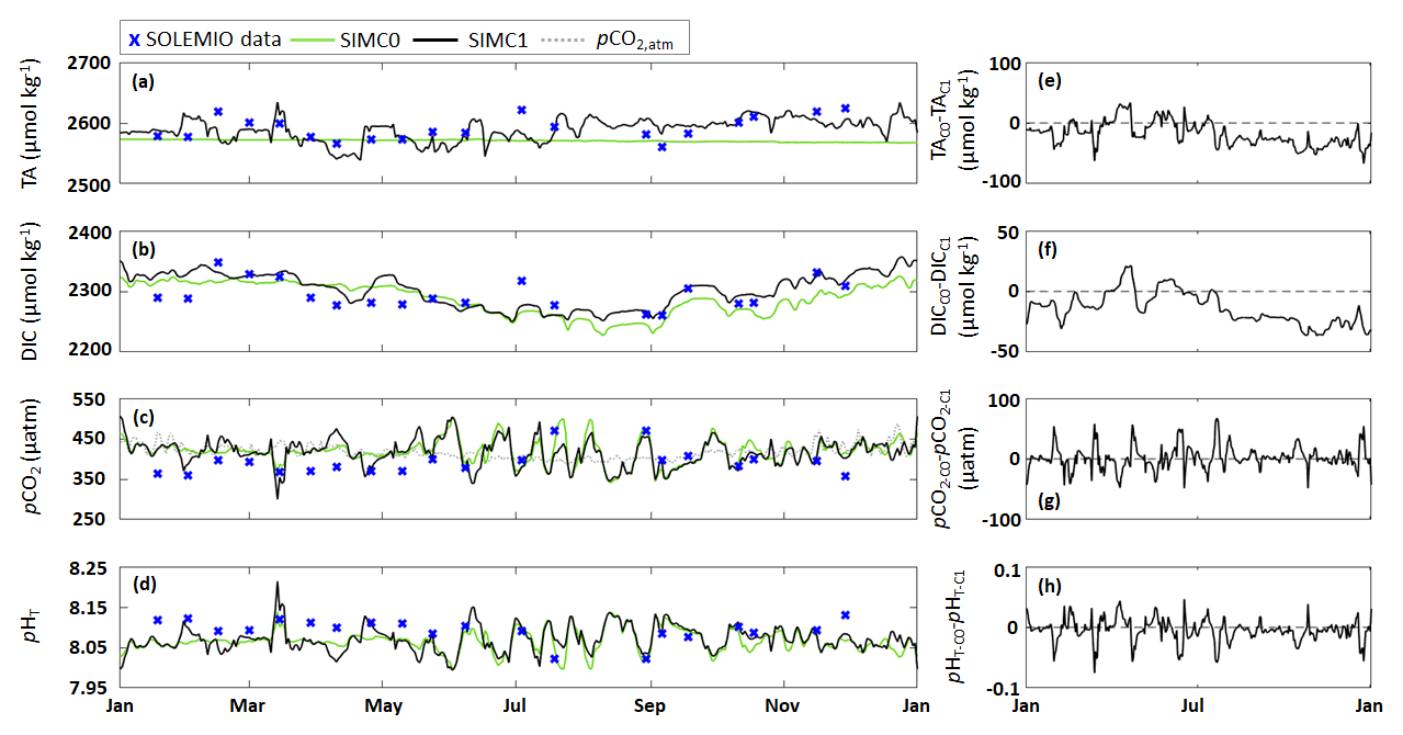
Figure 3 (a–d) Comparison of model outputs from the SIMC0 (autochthonous formulation) and SIMC1 (allochthonous formulation) model runs showing daily averages of (a) TA, (b) DIC, (c) seawater pCO₂ and CAV atmospheric pCO₂, and (d) pH_T. (e–h) Differences between SIMC0 and SIMC1 outputs for each variable (VARC0 − VARC1).

3 Results

3.1 Carbonate system variables

First, we performed an initial qualitative evaluation of Eco3M_MIX-CarbOx, comparing the output of SIMC0 (using the autochthonous TA formulation) and SIMC1 (using allochthonous TA formulation) for TA, DIC, pCO₂, and pH_T to the corresponding SOLEMIO surface data for 2017 (Fig. 3a–d). Next, we used four statistical indicators to compare model outputs and SOLEMIO data quantitatively: the percentage bias (%BIAS); the average error (AE); the average absolute error (AAE) and the root mean square deviation (RMSD, also referred to as the root mean square error (RMSE) in the literature). They were used with both Eco3M_MIX-CarbOx simulations, SIMC0 and SIMC1 (Table 1), and the reference Eco3M-CarbOx simulation (Lajaunie-Salla et al., 2021). By comparing the statistical indicators obtained for SIMC0, SIMC1, and Eco3M-CarbOx, we obtained an indication of how changes in the carbonate variable formulation affected the results. The statistical-indicator calculation is detailed in Appendix C.

The different TA formulations yielded very different model outputs for DIC, pCO₂, and pH_T (Fig. 3f–h). TA observations varied between 2560.8 and 2623.9 µmol kg⁻¹, with no apparent seasonal pattern (Fig. 3a). This variability is successfully represented by SIMC1 but not by SIMC0 (SIMC1 range: 2540 to 2635 µmol kg⁻¹). SIMC0 produces TA values that show a gradual and near-linear decrease from 2578 µmol kg⁻¹ in early January to 2572 µmol kg⁻¹ at the end of the year. The differences between SIMC0 and SIMC1 are most pronounced between August and December, where SIMC1 delivers systematically higher TA values compared to SIMC0 (Fig. 3e).

With regard to DIC, both SIMC0 and SIMC1 are capable of reproducing the seasonal variability present in the in situ data. From November to April, DIC has higher values (around 2320 µmol kg⁻¹ in both simulations), with lower values during the rest of the year (both have a minimum in August – SIMC0: 2234 µmol kg⁻¹ and SIMC1: 2254 µmol kg⁻¹; Fig. 3b). At the beginning of the year, SIMC1 seems to be closer to the observations than SIMC0, which shows fewer variations (e.g., SIMC1 appears to be better at reproducing the decrease visible at the end of April). Differences between SIMC0 and SIMC1 for DIC are similar to those observed for TA (Fig. 3e, f), although, in absolute terms, they are only about half of what we observed for TA. Nevertheless, these results show that the choice of the TA formulation strongly affects the DIC model results (Fig. 3f).

The in situ pCO₂ data exhibit strong variations throughout the year, especially from May to November, which are well represented in both simulations (Fig. 3c). Between January and April, both simulations overestimate the in situ pCO₂ values: while the simulations both predict pCO₂ values close to the CAV atmospheric pCO₂ at about 415 µatm, pCO₂ observed at SOLEMIO is lower, indicating under-saturation. For both simulations, a strong decrease in pCO₂ is modeled on 15 March in response to a Rhône River intrusion in the BoM. This event is particularly marked in the SIMC1 model results, which show a decrease from 450 to 300 µatm (compared to a decrease from 415 to 358 µatm with SIMC0). While this decrease is also visible in the in situ data, it is more moderate (392 to 367 µatm).

Regarding pH_T, both simulations produced similar dynamics as for pCO₂ (Fig. 3d vs. 3c). Both simulations deliver good representations of the observed pH_T variations between May and November, while from January to April, both simulations underestimate the in situ data (in situ: 8.12 vs. simulations: 8.07). The Rhône River intrusion is also visible in the pH_T data, which exhibit a sudden increase. While both simulations show this increase, it is more pronounced in the SIMC1 results (increase from 8.04 to 8.21) compared to SIMC0 (8.07 to 8.14), but in both cases, it is larger than in the observations (8.09 to 8.12).

The differences between both simulations for pCO₂ and pH_T do not exhibit any noticeable trend (Fig. 3g, h). However, looking at the annual average, SIMC1 produces lower (higher) pCO₂ (pH_T) values compared to SIMC0, with a mean difference of 2.3 µatm ($-\mathrm{5}\times {\mathrm{10}}^{-\mathrm{3}}$). Moreover, for both variables, the differences between SIMC0 and SIMC1 are more pronounced at the beginning of the year.

Table 2 Comparison of the different model results to surface observations at SOLEMIO station for TA, DIC, seawater pCO₂, and pH_T. N represents the number of observations. Mean, SD, AE, AAE, and RMSD are in the same unit as the considered variable, i.e.,: µmol kg⁻¹ for TA and DIC and µatm for pCO₂. %BIAS is without a unit.

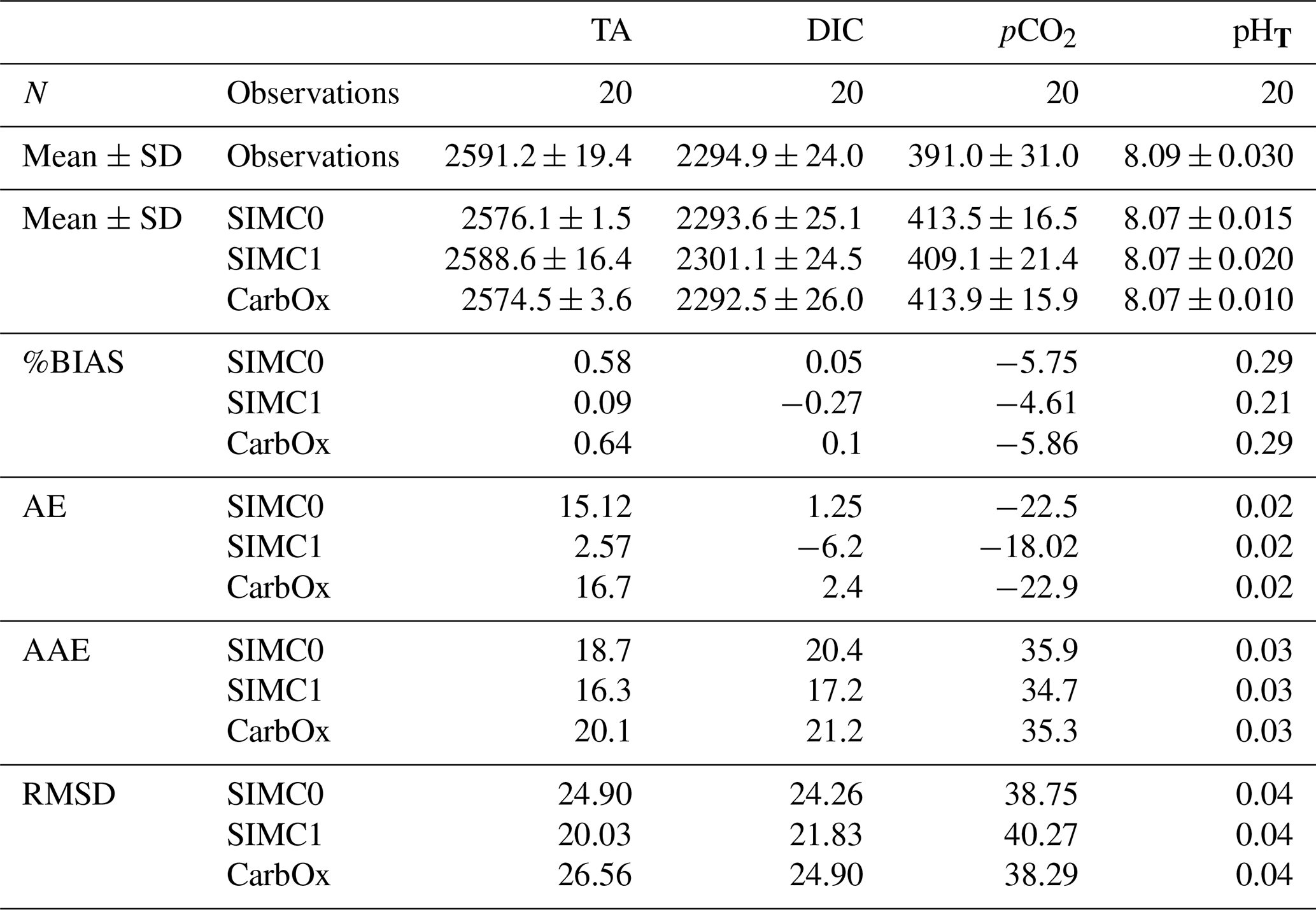
For statistical indicators, %BIAS values are systematically lower than 10 %, with the highest values being obtained for pCO₂ at∼6 %, while the remaining variables had values of <1 %. Similarly, pCO₂ had the highest RMSD, AAE, and AE, which suggests that this parameter is not as well represented in the model as the other variables. Furthermore, SIMC1 produced the best TA representation, resulting in the lowest values for %BIAS, AE, AAE, and RMSD (Table 2). Moreover, SIMC1 produced an annual mean TA that was closest to the observations. On the other hand, the SIMC0 and Eco3m-CarbOx results are fairly similar. SIMC0 produced a slightly better representation of TA compared to Eco3m-CarbOx (%BIAS, AE, AAE, and RMSD slightly lower). For pH_T, SIMC1 outperformed SIMC0 based on %BIAS (Table 2); however, AE, AAE, and RMSD values are similar for the three simulations. We then performed the calculation of statistical indicators for H⁺ concentration as, according to some authors (Kwiatkowski and Orr, 2018), comparing H⁺ concentrations is a better practice than comparing pH. Results are available in Appendix C. Based on Table C1, SIMC1 also outperformed SIMC0 based on AE and AAE. For studying DIC and pCO₂, the situation is less clear as the simulations performed differently for different indicators, making it difficult to pick a clear winner. Still, SIMC1 shows the best AAE and RMSD values for DIC and the best %BIAS, AE, and AAE for pCO₂. In conclusion, SIMC1 shows the best overall indicator values for the examined variables (more specifically, it outperformed the other simulations in 13 out of 20 indicator comparisons when including an H⁺ concentration comparison).

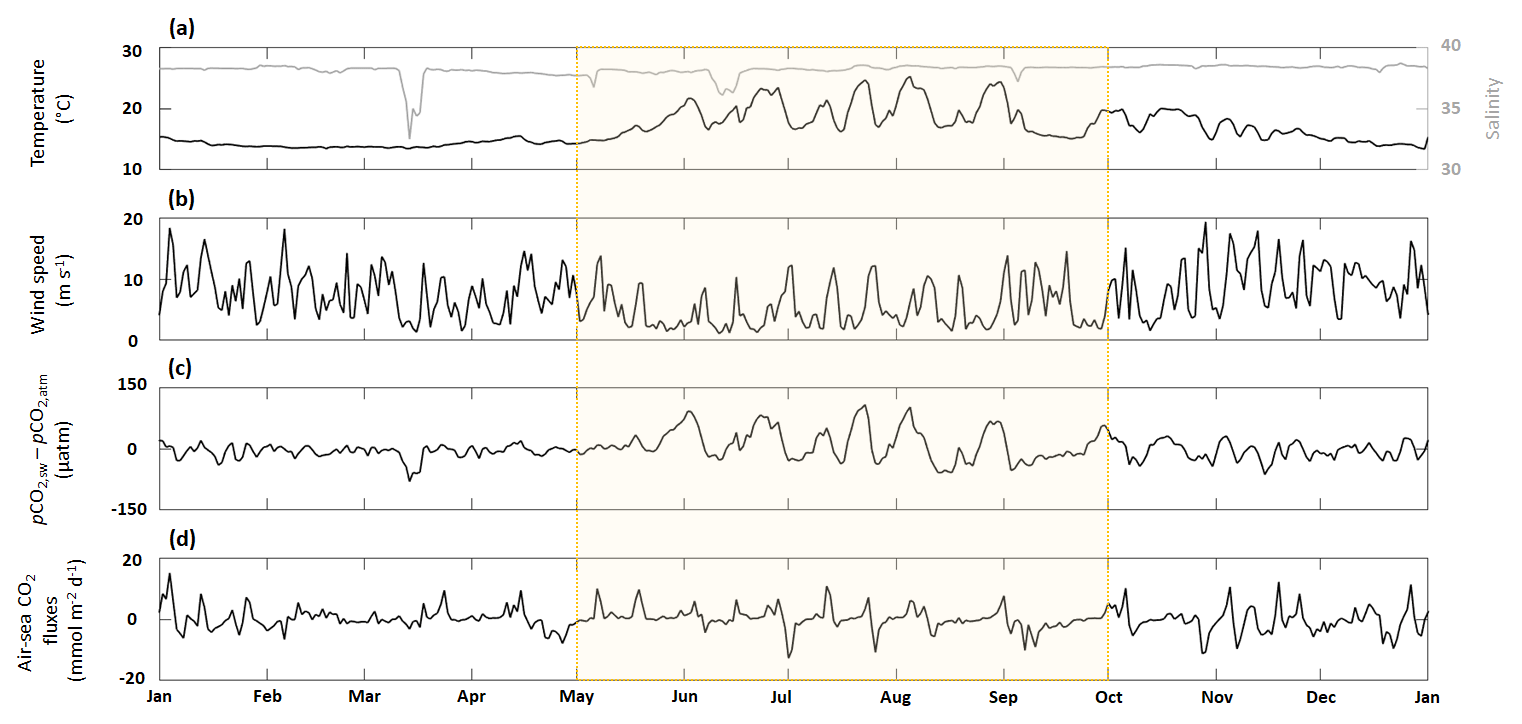
Figure 4 Time series of (a, e) in situ daily average sea surface temperature (black line) and salinity (gray line), (b, f) SIMC1 daily average wind speed, (c, g) the difference between SIMC1 daily average seawater pCO₂ and in situ daily average atmospheric pCO₂, (d, h) and SIMC1 daily average air–sea CO₂ fluxes (aeration process). The summer upwelling period (from 1 May to 1 October) is highlighted in yellow.

3.2 Air–sea CO₂ fluxes

Throughout 2017, temperature varied from 13.3 to 25.9 °C (Fig. 4a), with the highest variability visible during the summer upwelling period (SUP). Apart from four low-salinity events in March, May, June, and September (all corresponding to the Rhône River intrusions), the salinity remained close to its mean value of 38.1 (Fig. 4a).

Wind speed was highly variable, with several strong gusts, especially during winter, when wind speeds often exceeded 10 m s⁻¹ (Fig. 4b). Wind speed tends to be lower during summer and SUP, although these periods also show numerous strong wind events (>10 m s⁻¹).

The sea–air pCO₂ difference exhibits the same seasonality as temperature, with high positive values during summer while oscillating around zero during the rest of the year. In general, the sea–air pCO₂ difference combines the patterns from temperature, salinity, and wind speed, which are the main underlying forcings. The local minimum in March corresponds to an extremely low-salinity event (Fig. 4c). However, during the SUP, the sea–air pCO₂ difference is mostly driven by temperature, as seen from the high variability between May and October, which coincides with the largest temperature variations.

In contrast, air–sea CO₂ fluxes do not show any seasonality, with values oscillating about zero throughout the year (Fig. 4d), yielding an integrated total of −0.21 mmol m⁻² per year. Maximum positive values are obtained from November to March, when wind speeds are highest. Extreme negative values (−13 mmol m⁻² d⁻¹) can be seen in July, coinciding with high wind speed, negative sea–air pCO₂ difference, and a significant drop in temperature.

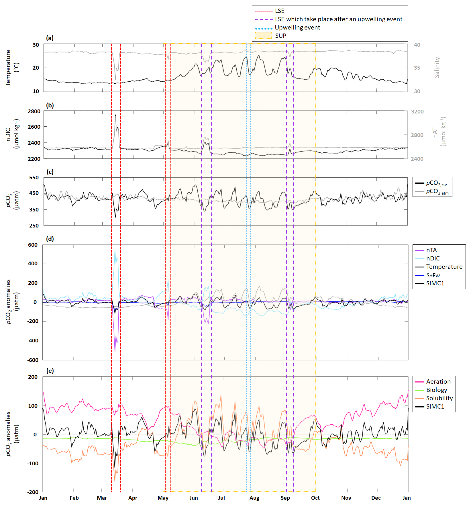
Figure 5 Time series for 2017 of daily average (a) in situ temperature and salinity; (b) modeled nDIC and nTA; (c) modeled seawater and in situ atmospheric pCO₂; (d) pCO₂ anomalies generated by DIC, TA, S+Fw, and temperature based on the approach in Lovenduski et al. (2007) (note: the dark-blue line is sometimes obscured by the black line, especially in March. An enlargement of panel (d) is available in Appendix D); and (e, j) pCO₂ anomalies generated by aeration, solubility, and biological processes based on the approach in Turi et al. (2014). LSE and an upwelling event have been highlighted. The summer upwelling period (SUP) is indicated by yellow shading.

3.3 Main drivers of pCO₂ dynamics

3.3.1 Annual scale

Following the approach from Lovenduski et al. (2007), we used temperature (Fig. 5a), salinity (S), freshwater inputs (Fw), salinity-normalized TA (nTA), and salinity-normalized DIC (nDIC) (Fig. 5b) contributions to identify the underlying dynamics in the observed pCO₂ variations (Fig. 5c). Seasonal variations in temperature (Fig. 5a) produce seasonal anomalies in pCO₂, with negative anomalies dominating from November to May and mostly positive anomalies throughout the remainder of the year (Fig. 5d). Anomalies generated by S+Fw do not exhibit any seasonality but remain close to zero throughout the year, unless there is an LSE, during which the anomalies turn negative (−101, −30, −40, and −20 µatm for the four LSE). Anomalies generated by nDIC show the opposite seasonal trend compared to the anomalies generated by temperature; i.e., from November to May the nDIC-generated anomalies are positive and are negative during the rest of the year. The four LSEs are also clearly visible in the nDIC-generated anomalies, which exhibit sharp increases (increases of 506, 253, 243, and 152 µatm, respectively). Also, nTA does not produce any seasonality in the anomalies but exhibits a sharp decrease during the four LSEs (decreases of 548, 242, 239, and 90 µatm, respectively).

Following the approach by Turi et al. (2014), we examined the effects of aeration, biological processes, and solubility on pCO₂ variability (Fig. 5e). Aeration produced anomalies very similar to those observed for nDIC (Fig. 5d): positive from November to May and negative during the rest of the year. Since CO₂ solubility is controlled by temperature and salinity, solubility-generated anomalies essentially follow the trends and seasonality seen in temperature- and S+Fw-generated anomalies (Fig. 5d): negative from November to May and mostly positive during the rest of the year (mean of +9.2 µatm).

The four LSEs are also visible in the solubility-generated anomalies generating strong decreases (Fig. 5e). However, only two LSEs are easily identifiable (on 15 March, with a drop from −41 to −163 µatm, and on 6 May, with a drop from 8 to −75 µatm), while the other two appear to be obscured by temperature-related counter-movements. Since aeration- and solubility-generated anomalies show opposite seasonality, they partly cancel each other out. While aeration seems to dominate from November to May (apart from LSE), solubility appears to dominate from May to November and during LSE. Biological processes are never the dominant driver of pCO₂ variations as they are systematically smaller (by a factor of 2 to 3) than aeration- and solubility-generated anomalies (Fig. 5e). Biology-induced anomalies are always negative, providing evidence that biological processes always decrease pCO₂.

3.3.2 During the summer upwelling period (SUP)

The SUP is characterized by significant temperature variations (Fig. 5a) due to periodic upwelling events. During the 2017 SUP, there were three LSEs, which will be excluded here as we discuss them in the following section. nTA is nearly constant during the SUP, while nDIC shows marked variations (Fig. 5b) that are directly linked to variations in DIC (see Sect. 3.1). pCO₂ is also highly variable during the SUP (Fig. 5c). Using the approach from Lovenduski et al. (2007) (Fig. 5d), the SUP is characterized by a strong contribution of temperature, which shows strong positive anomalies (maximum of 170 µatm reached on 5 August), and nDIC, which shows strong negative anomalies (minimum of −142 µatm reached on 24 July). S+Fw and nTA do not represent significant drivers, with anomalies remaining close to zero. Using the approach in Turi et al. (2014) (Fig. 5e), we can see that solubility is a major driver producing large-amplitude variations in the pCO₂ anomalies connected to similar variations in temperature (a drop in temperature causes the anomaly to change from positive to negative and vice versa) (Fig. 5a). Aeration, which mostly generates negative anomalies, counteracts solubility. During the SUP, we also observed an increase in the contribution of biological processes since associated anomalies are further decreased at the beginning of the period (from −22 µatm on 1 May to −40 µatm on 31 May).

Focusing on the upwelling event that took place between 23–27 July, we observe a sharp decrease in temperature (from 24.6 to 16.9 °C; Fig. 5a), no variation in nTA, and a slight increase in nDIC (from 2242 to 2269 µmol kg⁻¹; Fig. 5b). The event is also associated with a strong pCO₂ decrease (from 438 to 353 µatm; Fig. 5c). Using the approach in Lovenduski et al. (2007), we observed a decrease in the temperature-generated anomaly (from 148 µatm at the beginning of the event to 5 µatm at the peak of the event). At the same time, the nDIC-generated anomaly become less negative (from −142 µatm at the beginning of the event to −79 µatm at the peak of the event). Neither nTA nor S+Fw seem to have any significant impact on pCO₂ anomalies. Using the approach in Turi et al. (2014) (Fig. 5e), the upwelling event is characterized by a decrease in solubility-generated anomalies (from 79 µatm at the beginning of the event to −24 µatm at the end of the event). Anomalies generated by aeration and biological processes tend to become, respectively, positive and less negative at the end of the event (aeration: −45 to 3 µatm; biological processes: −30 to −20 µatm).

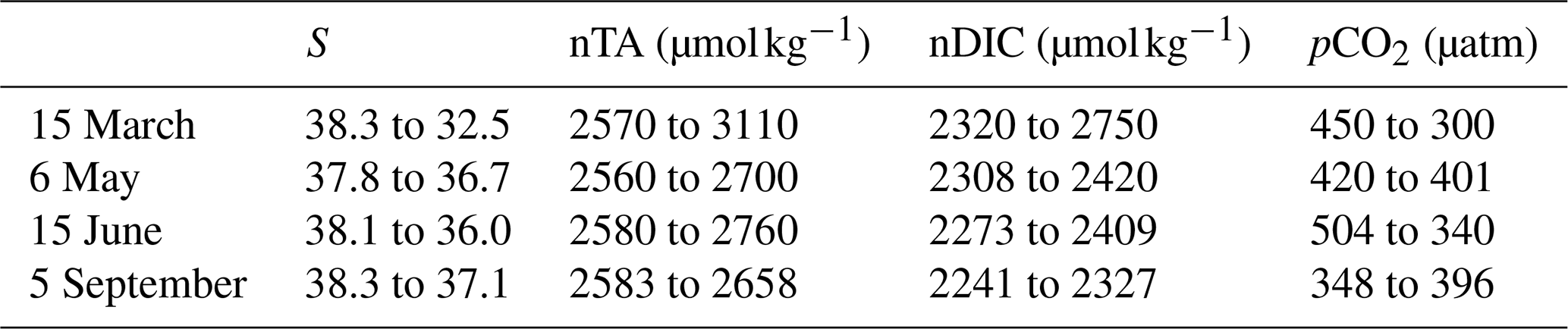
Table 3 Change in S, nTA, nDIC, and pCO₂ from before to during an LSE.

3.3.3 During a low-salinity event (LSE)

There were four LSEs during 2017: on 15 March, 6 May, 15 June, and 5 September. All four LSEs show similar patterns, namely a strong decrease in salinity (Fig. 5a), which in turn leads to an increase in both nTA and nDIC (Fig. 5, Table 3). Apart from the 5 September LSE, which shows an increase in pCO₂, the remaining LSEs coincide with significant pCO₂ decreases (Fig. 5c, Table 3).

When using the approach of Lovenduski et al. (2007), LSEs that do not take place immediately after an upwelling event (i.e., 15 March and 6 May) exhibit similar combinations of driver contributions; e.g., nTA and S+Fw create strong negative anomalies in both LSEs (with combined (nTA + S+Fw) contributions of −614 µatm on 15 March and −211 µatm on 6 May), which are partially canceled out by opposite nDIC contributions (547 µatm on 15 March and 235 µatm on 6 May). While temperature-generated anomalies showed no change during either event, they were still negative, and by adding their effect to those obtained for nTA and S+Fw, we obtain a combined effect of −656 µatm on 15 March and −241 µatm on 6 May.

LSEs that take place immediately after a summer upwelling event (i.e., 15 June and 5 September) show similar variations in salinity, nTA, nDIC, and pCO₂ but also show an increase in temperature (from 16.5 to 20.5 °C on 15 June and 17.5 to 19.8 °C on 5 September; Fig. 5a). Also, the factors driving the anomalies are similar to those for the non-upwelling-related LSEs discussed in the previous paragraph. The combined nTA and S+Fw anomalies (−260 µatm on 15 June and −108 µatm on 5 September) are partially compensated for by the nDIC contribution (171 and 22 µatm, respectively). Unlike for the previous events, we do see a significant temperature effect for the upwelling-related LSEs: temperature-generated anomalies are positive (45 µatm on 15 June and 53 µatm on 5 September) and support the nDIC contribution.

When following Turi et al. (2014) (Fig. 5e), all LSEs, with the exception of the 5 September LSE, are characterized by strong negative solubility-generated anomalies (−163 µatm on 15 March, −78 µatm on 6 May, and −55 µatm on 15 June), partially compensated for by positive aeration-generated anomalies (65, 97, and 8 µatm, respectively). The odd one out, which takes place on 5 September, shows a positive solubility-generated anomaly (27 µatm) and a negative aeration-generated anomaly (−30 µatm). In all four of the LSEs, biological processes did not have any significant impact on pCO₂ variations (anomalies generated by biological processes are 2 to 3 times lower than those generated by aeration or solubility).

4 Discussion

4.1 Impact of Rhône River inputs on TA variations

Due to its location near the Rhône River mouth, the BoM is particularly affected by freshwater inputs. In 2017, there were four LSEs in the BoM. Apart from being low in salinity, the Rhône River water entering the BoM also contains organic matter, nutrients, DIC, and alkalinity, with a mean TA of 2885 µmol kg⁻¹ (Schneider et al., 2007). This input adds up to the effect of biological processes. We have seen that TA measurements in the BoM exhibit significant variability throughout the year (Fig. 3a), although they exhibit no obvious seasonality. By considering autochthonous (i.e., dependent on biological processes only) and allochthonous (i.e., dependent on river inputs only) formulations of TA, we were able to isolate the effects of the biology and riverine inputs and quantify their relative importance for the TA variations seen in the BoM.

With the autochthonous formulation, TA remained fairly constant throughout the year, which is similar to the results obtained by Lajaunie-Salla et al. (2021). In contrast, the allochthonous formulation produced a much higher variability in TA that was close to in situ observations. Several authors suggested that biological processes could have a large effect on TA dynamics in coastal areas (Krumins et al., 2013; Gustafsson et al., 2014). These findings are not confirmed by our model results, where changes in TA due to biology did not exceed 5 µmol kg⁻¹ (Fig. 3a), which is insignificant compared to the changes attributed to other drivers, including riverine inputs. This suggests that TA variations in the BoM are mostly driven by allochthonous factors. The importance of allochthonous contributions to TA variations has already been highlighted by several authors at the Mediterranean Sea scale (Copin-Montegut, 1993; Schneider et al., 2007; Hassoun et al., 2015). Other important drivers in the Mediterranean include TA exchanges with the Atlantic Ocean and Black Sea, as well as TA inputs from sediments and rain. For the particular location of our study area, we only considered river contributions. Having neglected other allochthonous drivers seems to be justified by the results, which showed a close match to observations and a generally better representation of the other carbonate system variables since DIC, pCO₂, and pH_T are all closely related to TA (Fig. 3 and Table 2). Several studies of TA variations in the Mediterranean Sea have been conducted at the sub-basin-scale, yielding different TA–S correlations for different study areas (Cossarini et al., 2015; Hassoun et al., 2015). For instance, the correlation proposed for the northwestern Mediterranean Sea suggests that local TA dynamics are mainly controlled by evaporation. We did not include this in our study as the BoM is strongly impacted by the Rhône River. By focusing on a smaller area, we could provide a TA formulation that represents this particular part of the Mediterranean very well.

While our results seem to provide a realistic representation of TA dynamics in the BoM, we could have included other factors such as sediments, which have been shown to be important for TA dynamics, particularly in coastal areas (Brenner et al., 2016; Gustafsson et al., 2014). We plan to add TA supplies by sediments in our future work. Moreover, from a more conceptual perspective, the use of the present TA allochthonous formulation allowed us to manage two cases of salinity, namely S≤37.8 and S>37.8, with two different equations (Eqs. 5 and 6); however, the switch from one to another – in other words, crossing the threshold value – may lead to instabilities in TA representation. A solution to better manage the threshold-crossing case is to represent the Rhône River inputs more realistically. Here, we used two TA–S couples (TA and S at the mouth of the Rhône River and TA and S measured at SOLEMIO during the most significant Rhône River intrusion event) to obtain the dilution formulation. With this method, we do not take into account the seasonality of TA in the Rhône River, which can bring about significant variations (Fig. S2 and Table S3 of Supplement).

4.2 Impact of hydrodynamic processes on pCO₂ variations

4.2.1 Low-salinity events (LSEs)

The four LSEs observed in 2017 had several common characteristics: a salinity decrease (Fig. 5a) and apparent nTA and nDIC increases (Fig. 5b). Three of the four LSEs resulted in a pCO₂ decrease (15 March, 6 May, and 15 June; Fig. 5c). Rhône River intrusion events are often associated with a pCO₂ decrease since the introduced nutrients stimulate phytoplanktonic growth (Fraysse et al., 2014; Lajaunie-Salla et al., 2021). However, in our case, the decrease in pCO₂ observed on 15 March, 6 May, and 15 June was entirely caused by nTA and solubility effects (Fig. 5d, e). Generally, a TA increase is associated with a pCO₂ decrease that is proportional to the buffering state of the considered water mass (for high TA : DIC ratios, changes in pCO₂ are lower since the water mass is well buffered; Middelburg et al., 2020), which explains the negative pCO₂ anomalies associated with these three LSEs. Solubility depends on both salinity and temperature. Depending on the size and the duration of the Rhône River intrusion, the salinity effect on solubility can vary. When salinity decreases, the solubility of CO₂ in seawater also decreases, which results in a decrease in pCO₂ (Middelburg, 2019). The effects of temperature on solubility vary throughout the year. For instance, during the 15 March and 6 May LSEs, temperatures were low and fairly constant (Fig. 5a) and therefore only contributed a small amount to the negative anomaly (Fig. 5d). In contrast, for the 15 June LSE, temperature caused a positive pCO₂ anomaly (Fig. 5d). This difference can be explained by the fact that the 15 June LSE took place right after an upwelling event, probably facilitated by the Marseille eddy presence near the BoM, which tends to be observed just after mistral events (Fraysse et al., 2014). While the temperature dropped as a result of the upwelling, once the event was over, the temperature increased again, which caused the observed positive pCO₂ anomaly. Despite this positive temperature-related anomaly, the overall anomaly remained negative due to the strong effects of salinity and nTA during the LSE (Fig. 5c).

The 5 September LSE was associated with a pCO₂ increase (Fig. 5c) caused by nDIC and solubility effects (Fig. 5d, e): as salinity and nTA contributions remain weak, they are completely counterbalanced by nDIC and temperature contributions, resulting in an increase in pCO₂. During the 5 September LSE, observed salinity and temperature showed opposite patterns: the decrease in salinity is associated with an increase in temperature, and the increase in salinity after the peak of the LSE is associated with a temperature decrease (Fig. 5a). Unlike for the 15 June LSE, the temperature increase seen during the 5 September event was not caused by the end of the preceding upwelling event as the temperature was decreasing right after the LSE peak (Fig. 5a). We assume that this temperature increase was instead caused by the intruding Rhône River water, which brought about the observed pCO₂ increase (pCO₂ increases exponentially with temperature; Middelburg, 2019).

In all four LSEs, biological processes did not have any significant impact on pCO₂ variations (Fig. 5e). To interpret this result, it is important to consider the assumptions used by Eco3M_MIX-CarbOx (Sect. 2.2). Rhône River intrusions can significantly modify the biogeochemistry of the bay as they are typically associated with temperature and salinity changes and TA, DIC, and nutrient inputs (Gatti et al., 2006; Fraysse et al., 2014; Lajaunie-Salla et al., 2021). Due to its 0D configuration, Eco3M_MIX-CarbOx only represents temperature and salinity changes and TA inputs (only if the allochthonous formulation is used for the latter; Fig. 1). For the studied events, linking measured surface salinity to measured DIC (Appendix E) showed that the four events are not systematically associated with a DIC increase at SOLEMIO even though the Rhône River mouth DIC value (2877 µmol kg⁻¹ – the value calculated by using TA and pH from Schneider et al. (2007) and Aucour et al. (1999), respectively) is much higher than the mean value at the station (2294.9 µmol kg⁻¹). Based on this observation, we can assume that, for DIC, the riverine signal is quickly lost when moving away from the Rhône River mouth and does not reach SOLEMIO station. Contrarily to TA, which is mainly affected by Rhône River inputs in the area, DIC is impacted by air–sea CO₂ exchanges and biological processes, which can explain this pattern. However, for more realism and as these inputs could affect pCO₂ variations by increasing the nDIC contribution, considering them could be an interesting addition to the present configuration. Moreover, linking measured surface salinity to measured nutrient concentrations (Appendix E) showed that only the first and last events (15 March and 5 September, respectively) have an impact on nutrient concentrations at SOLEMIO, with the first event being the most significant. Lajaunie-Salla et al. (2021) showed that these nutrient inputs led to an increase in chlorophyll concentration. This phytoplankton growth leads to a further decrease in pCO₂, which means that, by neglecting this, we possibly underestimated the importance of biological processes, especially of autotrophic processes, during these Rhône River intrusions.

4.2.2 Summer upwelling period (SUP)

During the SUP, regardless of whether there is an LSE, pCO₂ variations mostly depend on temperature and nDIC, which tend to produce anomalies of opposite signs (Fig. 5d). Temperature was highly variable during the SUP due to the succession of upwelling events, which explains its significant contribution to pCO₂ variations. nDIC contribution can be defined as the sum of aeration and biological-process contributions. During the SUP, biological processes represent 29 % of DIC variations (with 14 % attributed to primary production and 15 % to respiration; results not shown). The remaining 71 % are contributions by aeration. While the contribution of aeration decreased during summer, this decrease was compensated for by a 9 % increase in the contribution by biological processes (Fig. 5e). The maximum negative anomaly generated by biological processes occurred at the beginning of the SUP, on 31 May (Fig. 5e), which is evidence that biological processes and, more precisely, autotrophic processes are enhanced during late spring. This feature is explained by the change in organisms' limitations. At the end of spring, organisms are less limited by temperature and light. Nevertheless, the overall contribution of biological processes was low compared to the contributions of aeration and temperature. This agrees with observations by Wimart-Rousseau et al. (2020a) and Lajaunie-Salla et al. (2021), who showed that pCO₂ variations and associated CO₂ fluxes are mostly driven by temperature in the BoM.

We showed that upwelling events were associated with strong decreases in pCO₂ (Fig. 5c), mostly as a result of temperature changes. The associated decrease in temperature further decreased pCO₂. This feature is only observed during upwelling events in summer when both temperatures and pCO₂ are high (Fig. 5a, c), stressing the importance of upwelling events for these variables. During upwelling events, aeration-generated anomalies change sign and become positive (Fig. 5e). The observed decrease in temperature resulted in a decrease in seawater pCO₂ to below atmospheric levels, thereby facilitating the absorption of atmospheric CO₂, which caused the reversal in terms of the sign of the aeration-generated anomaly. During upwelling events, the contribution by biological processes is low compared to temperature and aeration, which both varied significantly (Fig. 5e). While upwelling events only occur at very specific locations (Côte Bleue and Calanques de Marseille) in our study area, they impact the temperature of the entire BoM (Pairaud et al., 2011). However, upwelling events also bring nutrients and DIC to the surface. In Eco3M_MIX-CarbOx, these effects are not considered, and upwelling events are only represented through temperature decreases in the volume. During the SUP, by linking surface temperature measurements and surface DIC and nutrient concentration measurements at SOLEMIO (Appendix E), we showed that (i) among the upwelling events, only two (at the beginning of July and in mid-September) are linked to a noticeable DIC variation, and (ii) surface nutrient concentration dynamics seem to be only slightly affected by upwelling events (nutrient concentrations remain close to 0 most of the time), explained by the fact that, when the upwelling takes place, nutrients which are upwelled are quickly consumed by the phytoplankton present in the area, thus not systematically reaching the station. Even though the effect of upwelling events on DIC and nutrient concentration seems to be limited at SOLEMIO station, it may be interesting to consider them for more realism as the temporal coverage of SOLEMIO measurements remains low (15 d), and we cannot exclude the fact that an impact can be observed but not caught by the measurements. Indeed, even if low, a nutrient input can promote primary production (Fraysse et al., 2013) then increase the contribution of biological processes (especially of autotrophic processes), resulting in a stronger decrease in pCO₂, while DIC inputs would increase the importance of nDIC, thereby reducing the decrease in pCO₂ associated with these events.

4.3 Air–sea CO₂ fluxes

We have shown that air-0sea CO₂ fluxes oscillated between −13 and 15 mmol m⁻² d⁻¹ (Fig. 4d), which is a range similar to the one obtained by Wimart-Rousseau et al. (2020a) (−15 and 10 mmol m⁻² d⁻¹), suggesting that our model correctly represents the range of variations in air–sea CO₂ daily flux values during the year. CO₂ sinks associated with upwelling events (Lajaunie-Salla et al., 2021) are reproduced by our model. By calculating the daily mean value of air–sea CO₂ fluxes during the SUP, we obtained a positive value of 0.15 mmol m⁻² d⁻¹ (or 24.2 mmol m⁻² for the entire SUP). To examine this result in more detail, we performed a sensitivity analysis of our air–sea CO₂ flux calculation (see Appendix F for details), which allowed us to identify the contributions of all relevant parameters (Table 4).

Table 4 Results of the sensitivity analysis showing the effect of varying the relevant parameters by 10 %.

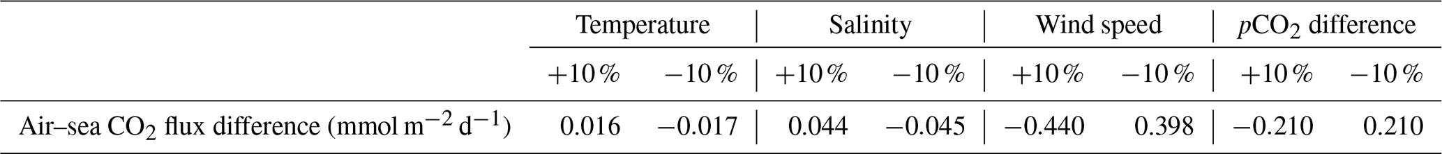
On average, air–sea CO₂ flux values during the SUP were mostly driven by the wind speed term, followed by sea–air pCO₂ differences, salinity, and finally temperature. According to Eqs. (8) and (9), wind speed, salinity, and temperature only affect the magnitude of air–sea CO₂ fluxes, while their sign is determined by the sea–air pCO₂ difference, which also impacts their magnitude significantly (Table 4). We have shown that, during the SUP, this difference is mostly driven by temperature since seawater pCO₂ variations are controlled by temperature at this time (Fig. 5d, e). A realistic representation of seawater pCO₂ is crucial to calculate air–sea CO₂ fluxes. Since seawater pCO₂ variations were correctly represented by the model during the SUP (Fig. 3c), the modeled air–sea CO₂ fluxes during the SUP should be reliable.

Over the entire year, air–sea CO₂ fluxes in the BoM essentially evened out, yielding only a slightly negative balance of −0.21 mmol m⁻² per year. This is much lower than the −803 mmol m⁻² per year suggested by Wimart-Rousseau et al. (2020a). The reason for this discrepancy may be related to the fact that our model overestimates seawater pCO₂ during winter, resulting in a sea–air difference close to zero (Fig. 4d). As a result, despite strong winds and low temperatures which would favor CO₂ absorption (Middelburg, 2019), the winter CO₂ sink is not well represented.

Seawater pCO₂, air–sea CO₂ fluxes, and DIC are closely connected (Appendix B). In Eco3M_MIX-CarbOx, aeration is simulated by applying Eq. (8) to 1 m³ of surface water at SOLEMIO station, which tends to overestimate the impact of the aeration process on DIC and, due to the close link between DIC and pCO₂, also on pCO₂. Indeed, when the aeration process is applied to this small volume, the balance between the atmosphere and the volume is quickly reached, which then impacts the representation of pCO₂. To overcome this problem, we need to consider a larger layer of water on which the aeration process is applied. Consequently, we ran a simulation in which we considered a larger thickness of water (H=30.5 m, annual mean value of the mixed-layer depth in the area; Eq. 8) on which to apply the aeration process. This simulation and its results are described in the Supplement. By increasing the volume on which the aeration process is applied, the annual mean value of air–sea CO₂ fluxes is more realistic (−113.6 mmol m⁻² yr⁻¹) but, still, much lower than the one obtained by Wimart-Rousseau et al. (2020a) in the area. In fact, to represent the air–sea CO₂ fluxes, especially their annual mean value, in a more realistic way, we must consider, on the one hand, a realistic volume of water on which the aeration process is to be applied and, on the other hand, all the processes that take place in the water column and impact this flux, especially vertical mixing and matter transfer to the bottom of the water column. Consequently, in the present state, Eco3M_MIX-CarbOx is unable to represent the annual cycle of air–sea CO₂ fluxes. Overcoming this problem requires the switch to a 3D configuration, which is planned for our future work.

Most studies that investigated air–sea CO₂ fluxes and other carbonate system variables in various Mediterranean locations at different locations (Ligurian Sea, North Adriatic Sea, BoM) were based on measurements only and concluded that their study areas acted as CO₂ sinks during their study periods (e.g., Begovic, 2001; De Carlo et al., 2013; Ingrosso et al., 2016; Urbini et al., 2020; Wimart-Rousseau et al., 2020a). To the best of our knowledge, the only other study examining air–sea CO₂ fluxes in the BoM using a modeling approach was conducted by Lajaunie-Salla et al. (2021) using the Eco3m-CarbOx model, which is also dimensionless and based on a 1 m³ volume like Eco3M_MIX-CarbOx and therefore also tends to underestimate the yearly fluxes. Most modeling studies have focused on larger scales and have employed at least 1D models. For instance, D'Ortenzio et al. (2008) used a coupled 1D model and found that the Mediterranean Sea, as a whole, was nearly balanced as the western and eastern basins act as a CO₂ sink and source, respectively, and therefore cancel each other out. Using a 3D coupled model and looking at even larger scales, Bourgeois et al. (2016) provided a complete analysis of the air–sea CO₂ fluxes in various coastal environments and have shown that they represent 4.5 % of the anthropogenic CO₂ uptake of the global ocean. The 3D models typically allow more realistic representations of the water column; they would allow us to (i) consider a more realistic water column (volume and processes which impact it) to perform our air–sea CO₂ flux calculations, (ii) consider autochthonous and allochthonous contributions to TA variations, and (iii) consider the effects of nutrients and DIC inputs from the Rhône River intrusions and local upwellings. Nevertheless, the dimensionless model also offers some advantages, including a short simulation time and easy adaptability, which allowed us to provide a detailed analysis of drivers of seawater pCO₂ variations, particularly during specific hydrodynamic processes typical for the BoM. This type of study is still uncommon in the area as few of studies have investigated the carbonate system dynamics, especially the pCO₂ variation drivers, and this would have been a tedious task to realize in 3D (i.e., longer simulations and isolation of the pCO₂ variation drivers' contributions are more difficult due to the complexity of the model).

5 Conclusion

Using the concept of the dimensionless Eco3M-CarbOx biogeochemical model as a starting point, we developed a new planktonic ecosystem model which contains, in addition to mixotroph organisms, a modified version of the carbonate module described by Lajaunie-Salla et al. (2021) to represent the carbonate system variables more realistically. First, we improved the parameterization of TA by developing two different formulations: (i) an autochthonous formulation that only considers biological contributions to TA variations and (ii) an allochthonous formulation that only depends on salinity, thus considering riverine contributions to TA variations. A comparison of both TA formulations showed that TA variations in the BoM were mostly due to allochthonous contributions. Then, we adapted the allochthonous formulation for modeling TA variations in the BoM, which yielded a helpful tool to complement the low-frequency in situ measurements. We use this new formulation to study air–sea CO₂ fluxes and seawater pCO₂ variations at SOLEMIO station in 2017, focusing on two hydrodynamic processes that are typical for the BoM: (i) Rhône River intrusions and (ii) summer upwelling events.

During the SUP, our model represented the CO₂ sinks generated by summer upwelling events, which are suggested by Lajaunie-Salla et al. (2021), and identified the underlying drivers of CO₂ variability. Furthermore, our model was able to simulate the expected decrease in pCO₂ associated with summer upwelling events (Lajaunie-Salla et al., 2021). This decrease was mainly generated by temperature effects on pCO₂. LSEs were also represented by the model. They often generated a decrease in pCO₂ as a result of the decreasing salinity and increasing TA, especially when those two contributions were not counterbalanced by temperature effects. However, in winter, the model was unable to reproduce the undersaturation seen in seawater pCO₂ measurements at SOLEMIO station and rather overestimated it. As a result, the present configuration of Eco3M_MIX-CarbOx is unable to reproduce the commonly observed seasonality of air–sea CO₂ fluxes in the northwestern Mediterranean. This pattern directly impacts our estimates of the overall yearly air–sea CO₂ flux as, even if the model clearly identifies the bay as a CO₂ sink, it does not allow us to reproduce the observed mean annual value of air–sea CO₂ fluxes (our model: −0.21 mmol m⁻² per year vs. model of Wimart-Rousseau et al. (2020a): −803 mmol m⁻² per year).

The present work clearly highlighted the limitations of dimensionless models. Although this type of model possesses some advantages that facilitate an improved understanding of complex coastal systems, it has clear limitations when it comes to the representation of specific processes or variables, with obvious impacts on the results. The accuracy could be improved by employing a 3D coupled model, which would allow us to (i) improve our representation of air–sea CO₂ fluxes by applying them to the whole water column, (ii) improve our representation of TA by considering autochthonous and other allochthonous sources, and (iii) improve our representation of LSE and upwelling events by allowing us to consider the inputs of nutrients and DIC.

Appendix A: State equation process description

Table A1 Description of state equation processes.

Appendix B: pH_T and pCO₂ calculation

The calculation method performed in the Eco3M_MIX-CarbOx model to obtain pH_T and pCO₂ is detailed below. As specified in Sect. 2, we used the method introduced by Lajaunie-Salla et al. (2021), which relies on CO2SYSv3 (Sharp et al., 2020), software originally developed by Lewis and Wallas (1998) to resolve the carbonate system using two of its four representative variables. This Appendix aims to complete Appendix A from Lajaunie-Salla et al. (2021) by providing some corrections. It also introduces the possibility of choosing between two types of TA formulations (autochthonous or allochthonous) to perform the calculation of pH_T and pCO₂.

B1 Equilibrium constant and conservative element concentration calculations

In the following formulations, S represents the practical salinity.

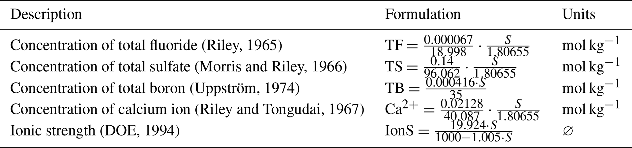
B1.1 Conservative element concentrations and ionic strength

Table B1 Formulations of conservative element concentrations and ionic strength.

B1.2 Equilibrium constants

In the following formulations, T represents the temperature value converted to Kelvin (i.e., T (°C) +273.15).

K_F (mol kg⁻¹): HF dissociation constant (Dickson and Riley, 1979b)

$$\begin{array}{}\text{(B1)}& \begin{array}{rl}& \ln \left(K_{\mathrm{F}}\right)={\displaystyle \frac{\mathrm{1590.2}}{T}}-\mathrm{12.641}+\mathrm{1.525}\cdot {\text{IonS}}^{\mathrm{0.5}}\\ & K_{\mathrm{F}}=\exp \left(\ln \left(K_{\mathrm{F}}\right)\cdot \left(\mathrm{1}-\mathrm{0.001005}\cdot S\right)\right)\end{array}\end{array}$$

K_F is expressed on the free pH scale.

K_S (mol kg⁻¹): HSO${}_{\mathrm{4}}^{-}$ dissociation constant (Dickson, 1990a)

$$\begin{array}{}\text{(B2)}& \begin{array}{rl}\ln {\left(K_S\right)}_{\mathrm{temp}}& =-{\displaystyle \frac{\mathrm{4276.1}}{T}}+\mathrm{141.328}-\mathrm{23.093}\cdot \ln \left(T\right)\\ & +\left(-{\displaystyle \frac{\mathrm{13}\mathrm{856}}{T}}+\mathrm{324.57}-\mathrm{47.986}\cdot \ln \left(T\right)\right)\cdot {\text{IonS}}^{\mathrm{0.5}}\\ \ln \left(K_S\right)& =\ln {\left(K_S\right)}_{\mathrm{temp}}+\left({\displaystyle \frac{\mathrm{35}\mathrm{474}}{T}}-\mathrm{771.54}+\mathrm{114}\mathrm{723}\cdot \ln \left(T\right)\right)\\ & \cdot \text{IonS}-{\displaystyle \frac{\mathrm{2698}}{T}}\cdot {\text{IonS}}^{\mathrm{1.5}}+{\displaystyle \frac{\mathrm{1776}}{T}}\cdot {\text{IonS}}^{\mathrm{2}}\\ K_S& =\exp \left(\ln \left(K_S\right)\cdot \left(\mathrm{1}-\mathrm{0.001005}\cdot S\right)\right)\end{array}\end{array}$$

K_S is expressed on the free pH scale.

K_B (mol kg⁻¹): B(OH)₃ dissociation constant (Dickson, 1990b)

$$\begin{array}{}\text{(B3)}& \begin{array}{rl}& \ln {\left(K_B\right)}_{\mathrm{temp}}=\\ & {\displaystyle \frac{-\mathrm{8996.9}-\mathrm{2890.53}\cdot S^{\mathrm{0.5}}-\mathrm{77.942}\cdot S+\mathrm{1.728}\cdot S^{\mathrm{1.5}}-\mathrm{0.0996}\cdot S^{\mathrm{2}}}{T}}\\ & +\mathrm{148.0248}+\mathrm{137.1942}\cdot S^{\mathrm{0.5}}\\ & \ln \left(K_B\right)=\ln {\left(K_B\right)}_{\mathrm{temp}}+\mathrm{1.62142}\cdot S\\ & +\left(-\mathrm{24.4344}-\mathrm{25.085}\cdot S^{\mathrm{0.5}}-\mathrm{0.2474}\cdot S\right)\cdot \ln \left(T\right)\\ & +\mathrm{0.053105}\cdot S^{\mathrm{0.5}}\cdot T\\ & K_B=\exp \left(\ln \left(K_B\right)\right)\end{array}\end{array}$$

K_B is expressed on the total pH scale.

K_ca (mol kg⁻¹)²: dalcite formation constant (Mucci, 1983)

$$\begin{array}{}\text{(B4)}& \begin{array}{rl}\log {\left(K_{\mathrm{ca}}\right)}_{\mathrm{temp}}& =-\mathrm{171.9065}-\mathrm{0.077993}\cdot T\\ & +{\displaystyle \frac{\mathrm{2839.319}}{T}}+\mathrm{71.595}\cdot \log \left(T\right)\\ \log \left(K_{\mathrm{Ca}}\right)& =\log {\left(K_{\mathrm{ca}}\right)}_{\mathrm{temp}}\\ & +\left(-\mathrm{0.77712}+\mathrm{0.0028426}\cdot T+{\displaystyle \frac{\mathrm{178.34}}{T}}\right)\\ & \cdot S^{\mathrm{0.5}}-\mathrm{0.07711}\cdot S+\mathrm{0.0041249}\cdot S^{\mathrm{1.5}}\\ & K_{\mathrm{ca}}={\mathrm{10}}^{\left(\log \left(K_{\mathrm{Ca}}\right)\right)}\end{array}\end{array}$$

K_e (mol kg⁻¹): H₂O dissociation constant (Millero, 1995)

$$\begin{array}{}\text{(B5)}& \begin{array}{rl}\ln \left(K_e\right)& =-{\displaystyle \frac{\mathrm{13}\mathrm{847.26}}{T}}+\mathrm{148.9802}-\mathrm{23.6521}\\ & \cdot \ln \left(T\right)+\left(-\mathrm{5.977}+{\displaystyle \frac{\mathrm{118.67}}{T}}+\mathrm{1.0495}\cdot \ln \left(T\right)\right)\\ & \cdot S^{\mathrm{0.5}}-\mathrm{0.01615}\cdot S\\ K_e& =\exp \left(\ln \left(K_e\right)\right)\end{array}\end{array}$$

K_e is expressed on the seawater pH scale (SWS).

K₀ (mol kg⁻¹ atm⁻¹): CO₂ solubility (Weiss, 1974)

$$\begin{array}{}\text{(B6)}& \begin{array}{rl}\ln {\left(K_{\mathrm{0}}\right)}_{\mathrm{temp}}& =-\mathrm{60.2409}+\mathrm{93.4517}\cdot {\displaystyle \frac{\mathrm{100}}{T}}\\ & +\mathrm{23.3585}\cdot \ln \left({\displaystyle \frac{T}{\mathrm{100}}}\right)\\ \ln \left(K_{\mathrm{0}}\right)& =\ln {\left(K_{\mathrm{0}}\right)}_{\mathrm{temp}}+S\cdot \left(\mathrm{0.023517}-\mathrm{0.023656}\right.\\ & \left.\cdot {\displaystyle \frac{T}{\mathrm{100}}}+\mathrm{0.0047036}\cdot {\left({\displaystyle \frac{T}{\mathrm{100}}}\right)}^{\mathrm{2}}\right)\\ K_{\mathrm{0}}& =\exp \left(\ln \left(K_{\mathrm{0}}\right)\right)\end{array}\end{array}$$

K₁ (mol kg⁻¹): H₂ CO₃ dissociation (Lueker et al., 2000)

$$\begin{array}{}\text{(B7)}& \begin{array}{rl}p{K}_{\mathrm{1}}& ={\displaystyle \frac{\mathrm{3633.86}}{T}}-\mathrm{61.2172}+\mathrm{9.6777}\cdot \ln \left(T\right)\\ & -\mathrm{0.011555}\cdot S+\mathrm{0.0001152}\cdot S^{\mathrm{2}}\\ K_{\mathrm{1}}& ={\mathrm{10}}^{\left(-p{K}_{\mathrm{1}}\right)}\end{array}\end{array}$$

K₁ is expressed on the total pH scale.

K₂ (mol kg⁻¹): HCO${}_{\mathrm{3}}^{-}$ dissociation (Lueker et al., 2000)

$$\begin{array}{}\text{(B8)}& \begin{array}{rl}p{K}_{\mathrm{2}}& ={\displaystyle \frac{\mathrm{471.78}}{T}}+\mathrm{25.929}-\mathrm{3.16967}\cdot \ln \left(T\right)\\ & -\mathrm{0.01781}\cdot S+\mathrm{0.0001122}\cdot S^{\mathrm{2}}\\ K_{\mathrm{2}}& ={\mathrm{10}}^{\left(-p{K}_{\mathrm{2}}\right)}\end{array}\end{array}$$

K₂ is expressed on the total pH scale.

B1.3 pH-scale conversion

The pH calculation is performed on the total scale. Accordingly, the previous constants are converted if necessary (i.e., expressed on total pH scale) using the following conversion factors. Except for K_S and K_F, which must be expressed on the free pH scale, the other equilibrium constants must be converted to the total pH scale.

Table B2 Formulation of pH-scale conversion factors.

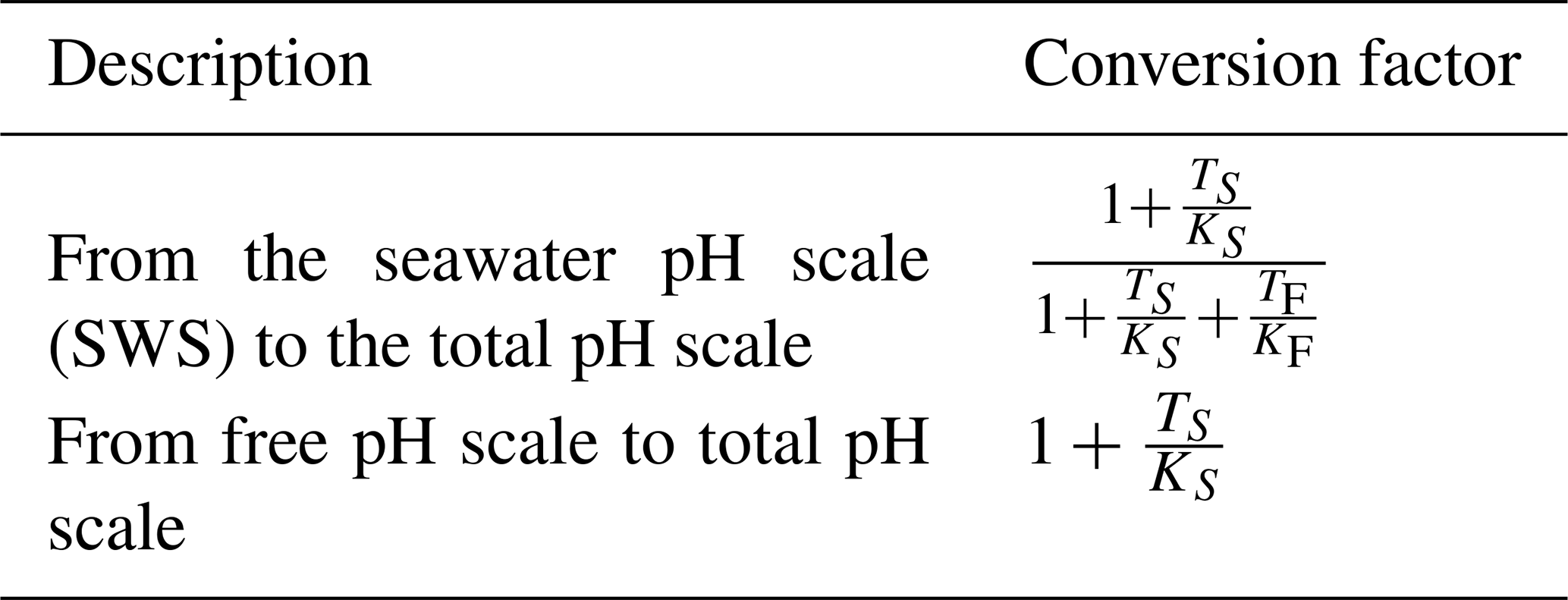
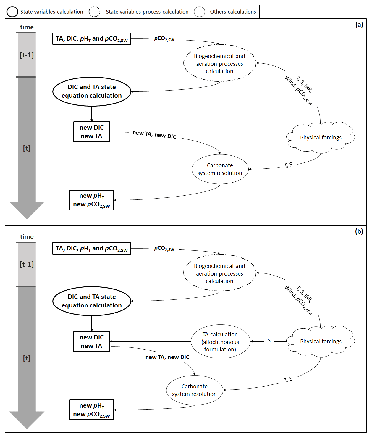
Figure B1 Flow diagram illustrating the steps needed to calculate pH_T and pCO₂ (a) using the autochthonous formulation (Eq. 4) and (b) with the allochthonous formulation (Eqs. 5 and 6). Physical forcings include temperature (T), salinity (S), solar irradiance (IRR), wind speed (wind), and atmospheric pCO₂ (pCO_2,ATM).

B1.4 Pressure correction

All the constants are corrected by the effect of hydrostatic pressure using the following formulations (Millero, 1995). We define T_K and T_C, which represent, respectively, the temperature in Kelvin and in Celsius. R represents the gas constant in mL bar⁻¹ K⁻¹ mol⁻¹ (R=83.1451 mL bar⁻¹ K⁻¹ mol⁻¹), and P represents the pressure in bar.

Corrected K_F (mol kg⁻¹)

$$\begin{array}{}\text{(B9)}& \begin{array}{rl}& K_{\mathrm{F}}\text{CorrFac}=\\ & {\displaystyle \frac{\left(\mathrm{9.78}+\mathrm{0.009}\cdot T_{\mathrm{C}}+\mathrm{0.0009429}\cdot T_{\mathrm{C}}^{\mathrm{2}}+\mathrm{0.5}\cdot \left(\frac{-\mathrm{3.91}+\mathrm{0.054}\cdot T_{\mathrm{C}}}{\mathrm{1000}}\right)\cdot P\right)\cdot P}{R\cdot T_{\mathrm{K}}}}\\ & K_{\mathrm{F}}=K_{\mathrm{F}}\cdot \exp \left(K_{\mathrm{F}}\text{CorrFac}\right)\end{array}\end{array}$$

Corrected K_S (mol kg⁻¹)

$$\begin{array}{}\text{(B10)}& \begin{array}{rl}& K_S\text{CorrFac}=\\ & {\displaystyle \frac{\left(\mathrm{18.03}-\mathrm{0.0466}\cdot T_{\mathrm{C}}-\mathrm{0.000316}\cdot T_{\mathrm{C}}^{\mathrm{2}}+\mathrm{0.5}\cdot \left(\frac{-\mathrm{4.53}+\mathrm{0.09}\cdot T_{\mathrm{C}}}{\mathrm{1000}}\right)\cdot P\right)\cdot P}{R\cdot T_{\mathrm{K}}}}\\ & K_S=K_S\cdot \exp \left(K_S\text{CorrFac}\right)\end{array}\end{array}$$

Corrected K_B (mol kg⁻¹)

$$\begin{array}{}\text{(B11)}& \begin{array}{rl}& K_B\text{CorrFac}=\\ & {\displaystyle \frac{\left(\mathrm{29.48}-\mathrm{0.1622}\cdot T_{\mathrm{C}}+\mathrm{0.002608}\cdot T_{\mathrm{C}}^{\mathrm{2}}+\mathrm{0.5}\cdot \left(-\frac{\mathrm{2.84}}{\mathrm{1000}}\right)\cdot P\right)\cdot P}{R\cdot T_{\mathrm{K}}}}\\ & K_B=K_B\cdot \exp \left(K_B\text{CorrFac}\right)\end{array}\end{array}$$

Corrected K_ca (mol kg⁻¹)²

$$\begin{array}{}\text{(B12)}& \begin{array}{rl}& K_{\mathrm{ca}}\text{CorrFac}=\\ & {\displaystyle \frac{\left(\mathrm{48.76}-\mathrm{0.5304}\cdot T_{\mathrm{C}}+\mathrm{0.5}\cdot \left(\frac{-\mathrm{11.76}+\mathrm{0.3692}\cdot T_{\mathrm{C}}}{\mathrm{1000}}\right)\cdot P\right)\cdot P}{R\cdot T_{\mathrm{K}}}}\\ & K_{\mathrm{ca}}=K_{\mathrm{ca}}\cdot \exp \left(K_{\mathrm{ca}}\text{CorrFac}\right)\end{array}\end{array}$$

Corrected K_e (mol kg⁻¹)

$$\begin{array}{}\text{(B13)}& \begin{array}{rl}& K_e\text{CorrFac}=\\ & {\displaystyle \frac{\left(\mathrm{20.02}-\mathrm{0.1119}\cdot T_{\mathrm{C}}+\mathrm{0.001409}\cdot T_{\mathrm{C}}^{\mathrm{2}}+\mathrm{0.5}\cdot \left(\frac{-\mathrm{5.13}+\mathrm{0.0794}\cdot T_{\mathrm{C}}}{\mathrm{1000}}\right)\cdot P\right)\cdot P}{R\cdot T_{\mathrm{K}}}}\\ & K_e\text{CorrFac}=K_e\cdot \exp \left(K_e\text{CorrFac}\right)\end{array}\end{array}$$

Corrected K₁ (mol kg⁻¹)

$$\begin{array}{}\text{(B14)}& \begin{array}{r}{K}_{\mathrm{1}}\text{CorrFac}=\\ & {\displaystyle \frac{\left(\mathrm{25.5}-\mathrm{0.1271}\cdot T_{\mathrm{C}}+\mathrm{0.5}\cdot \left(\frac{-\mathrm{3.08}+\mathrm{0.0877}\cdot T_{\mathrm{C}}}{\mathrm{1000}}\right)\cdot P\right)\cdot P}{R\cdot T_{\mathrm{K}}}}\\ & K_{\mathrm{1}}=K_{\mathrm{1}}\cdot \exp \left(K_{\mathrm{1}}\text{CorrFac}\right)\end{array}\end{array}$$

Corrected K₂ (mol kg⁻¹)

$$\begin{array}{}\text{(B15)}& \begin{array}{rl}& K_{\mathrm{2}}\text{CorrFac}=\\ & {\displaystyle \frac{\left(\mathrm{15.82}+\mathrm{0.0219}\cdot T_{\mathrm{C}}+\mathrm{0.5}\cdot \left(\frac{\mathrm{1.13}+\mathrm{0.1475}\cdot T_{\mathrm{C}}}{\mathrm{1000}}\right)\cdot P\right)\cdot P}{R\cdot T_{\mathrm{K}}}}\\ & K_{\mathrm{2}}=K_{\mathrm{2}}\cdot \exp \left(K_{\mathrm{2}}\text{CorrFac}\right)\end{array}\end{array}$$

B1.5 Fugacity factor

To perform the calculation of the fugacity factor (FugFac), we supposed that the pressure value is close or equal to an atmosphere (Weiss, 1974).

T represents the temperature in Kelvin. We define P_atm as the atmospheric pressure in bar: P_atm=1.01325 bar.

$$\begin{array}{}\text{(B16)}& \begin{array}{rl}& \ln \left(\text{FugFac}\right)=\\ & {\displaystyle \frac{\left(\left(-\mathrm{1636.75}+\mathrm{12.0408}\cdot T-\mathrm{0.0327957}\cdot T^{\mathrm{2}}+\mathrm{3.16528}\cdot \mathrm{0.00001}\cdot T^{\mathrm{3}}\right)+\mathrm{2}\cdot \left(\mathrm{57.7}-\mathrm{0.118}\cdot T\right)\right)\cdot P_{\mathrm{atm}}}{R\cdot T}}\\ & \text{FugFac}=\exp \left(\ln \left(\text{FugFac}\right)\right)\end{array}\end{array}$$

B2 pH_T and pCO₂ calculation

Solving the equations of the carbonate system requires knowledge of TA and DIC. Depending on the TA formulation used, the steps followed by the model to issue the new pH_T and pCO₂ are described in Fig. B1. If TA is calculated using Eq. (4), biogeochemical and aeration processes are applied as described in Eqs. (4) and (7) in order to deliver new ([t] time step values) TA and DIC: air–sea CO₂ fluxes are calculated from temperature, salinity, wind speed, atmospheric pCO₂, and seawater pCO₂, and the biogeochemical processes required, at least, temperature and solar irradiance to be computed. When calculated, processes are applied in the form of fluxes to the previous TA and DIC ([t−1] time step values) to solve their respective state equation. The pH_T and pCO₂ calculation is, then, performed using, in addition to TA and DIC, temperature and salinity data.

When TA is calculated using Eqs. (5) and (6), the biogeochemical and aeration fluxes computed during the first stage are only applied to DIC from the preceding time step, while TA is calculated after DIC based on the salinity data from the current time step. All subsequent steps are unchanged (Fig. B1b).

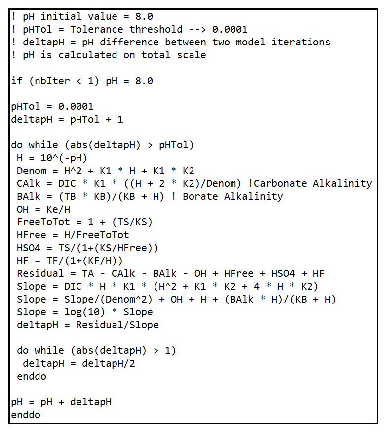
B2.1 pH_T calculation

pH_T is calculated using a buffering value (B) defined as the pH variation induced by an addition of acid or base to a specific solution (Van Slycke, 1922). In seawater, B can be expressed in terms of TA (Middelburg, 2019), which yields the following:

$$\begin{array}{}\text{(B17)}& B={\displaystyle \frac{\partial \text{TA}}{\partial {\text{pH}}_{\mathrm{T}}}}\iff \mathrm{\Delta }{\text{pH}}_{\mathrm{T}}={\displaystyle \frac{\partial \mathrm{TA}}{{\sum }_{i=\mathrm{1}}^n{B}_i}},\end{array}$$

where i represents a chemical species contributing to TA.

Accordingly, we calculate the pH_T difference between two model time steps (ΔpH_T) using an iterative method. We set the pH_T initial value to 8.0. We chose this value by considering the Mediterranean and Rhône River pH_T, which are, respectively, close and equal to 8.0. Finally, considering the fact that the measurement precision is rather close to 0.0004 (Clayton and Byrne, 1993), we set the tolerance threshold to 0.0001. The pH_T calculation is detailed in Fig. B2.

Figure B2 pH_T calculation.

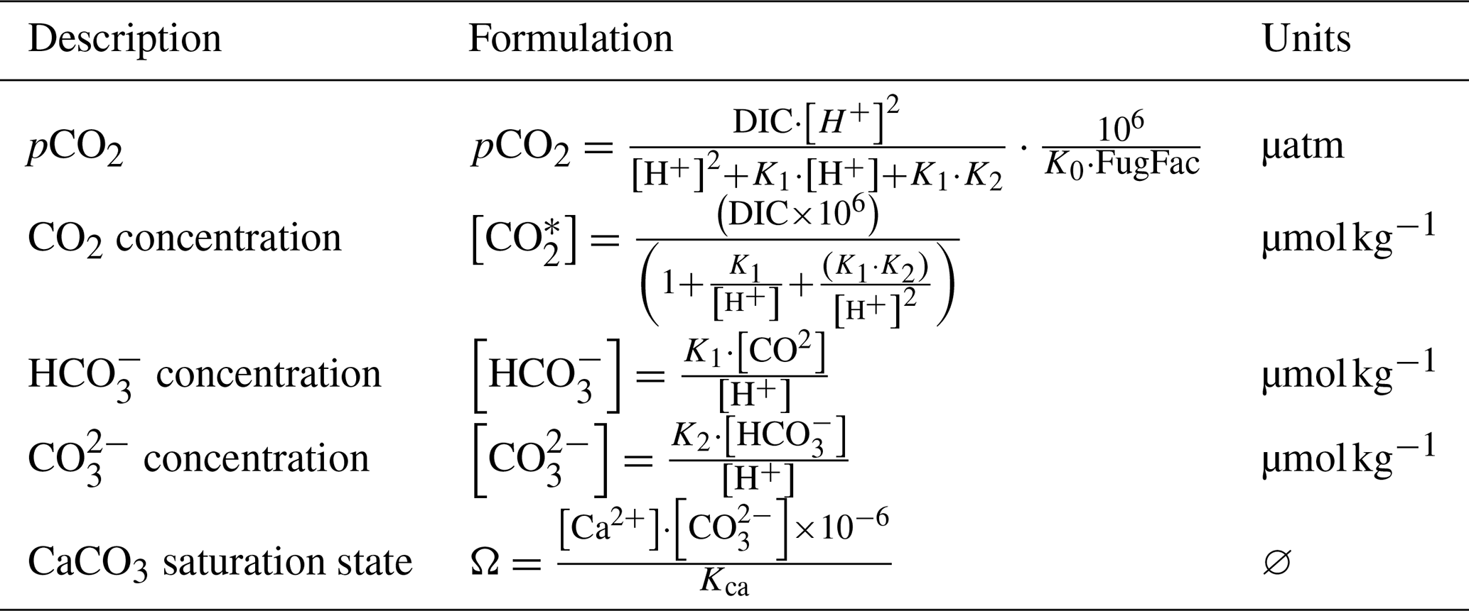
B2.2 pCO₂ and carbonate system species concentrations

pCO₂ is deducted using DIC, pH (via H⁺ concentration), and equilibrium constants. We also calculate the concentrations of CO₂, HCO${}_{\mathrm{3}}^{-}$, CO${}_{\mathrm{3}}^{\mathrm{2}-}$, and CaCO₃ saturation (Ω).

Table B3 Formulation of pCO₂ and carbonate system species concentrations. Note: To apply these formulations, DIC has to be expressed in mol kg⁻¹ and Ca²⁺ and CO${}_{\mathrm{3}}^{\mathrm{2}-}$ in µmol kg⁻¹.

Appendix C: Statistic indicator calculation and application to H⁺ concentration

We used four statistical indicators for the comparison between simulation and SOLEMIO data: the percentage bias (%BIAS), the average error (AE), the average absolute error (AAE), and the root mean square deviation (RMSD, also referred to as the root mean square error (RMSE) in the literature). They were used with two Eco3M_MIX-CarbOx simulations (SIMC0 and SIMC1) and the reference Eco3M-CarbOx simulation (Lajaunie-Salla et al., 2021). The %BIAS is calculated as follows:

$$\begin{array}{}\text{(C1)}& \mathrm{\%}\mathrm{BIAS}={\displaystyle \frac{{\sum }_{i=\mathrm{1}}^N\left(O_i-M_i\right)}{{\sum }_{i=\mathrm{1}}^N{O}_i}}\cdot \mathrm{100},\end{array}$$

where O represents the observations, and M represents the model results (Allen et al., 2007). This indicator allows us to quantify the model's tendency to under- or overestimate the observations. The closer the value is to 0, the better the model. Here, a positive %BIAS means that the model underestimated the in situ observations and vice versa. On an indicative basis, the %BIAS can be interpreted according to Maréchal (2004): absolute values of %BIAS allow us to assess the overall agreement between the model results and observations, and the agreement is considered to be excellent if %BIAS <10 %, very good if 10 % ≤ %BIAS <20 %, good if 20 % ≤ %BIAS <40 %, and poor otherwise. We based our calculation of AE, AAE, and RMSD on Stow et al. (2009). Together, these three statistical indicators provide an indication of model prediction accuracy.

$$\begin{array}{}\text{(C2)}& {\displaystyle }\mathrm{AE}={\displaystyle \frac{{\sum }_{i=\mathrm{1}}^N\left(O_i-M_i\right)}{n}}\text{(C3)}& {\displaystyle }\mathrm{AAE}={\displaystyle \frac{{\sum }_{i=\mathrm{1}}^N\left(\left|O_i-M_i\right|\right)}{n}}\text{(C4)}& {\displaystyle }\mathrm{RMSD}=\sqrt{{\displaystyle \frac{{\sum }_{i=\mathrm{1}}^N{\left(O_i-M_i\right)}^{\mathrm{2}}}{N}}}\end{array}$$

The three of them aim to measure the size of the discrepancies between model results and observations; the closer the value is to 0, the better the agreement between model results and observations. However, when interpreting AE, it is important to note that values near zero can be misleading because negative and positive discrepancies can cancel each other out. That is why it is important to calculate, in addition to AE, AAE and RMSD, which allow us to overcome this effect (Stow et al., 2009). Such as with %BIAS, a positive value of AE means that the model underestimated the in situ observations and vice versa. The model data are averaged using the mean of the output from the date in question ±5 d. Using the temporal mean and standard deviation of the model results allowed us to better account for the variability at SOLEMIO station.

Table C1 Comparing the different model results to surface observations at SOLEMIO station for H⁺ concentration. N represents the number of observations. Mean, SD, AE, AAE, and RMSD are in the same unit as the considered variable, i.e., mmol m⁻³ for H⁺ concentrations. %BIAS is without a unit.

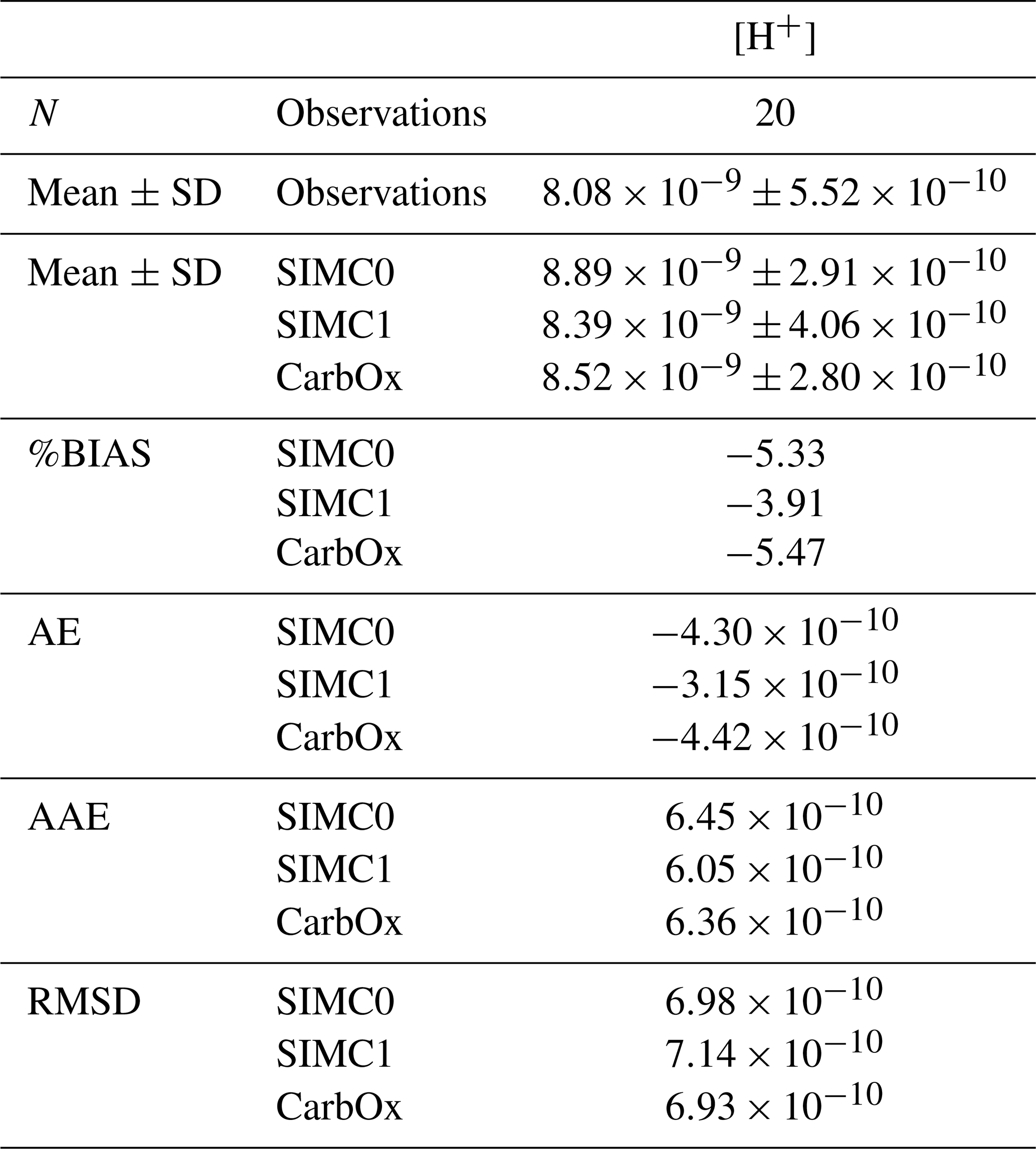
In addition to TA, DIC, pH_T, and pCO₂, statistical indicators were calculated for H⁺ concentrations (Table C1).

Appendix D: Time series of daily average pCO₂ anomalies generated by DIC, TA, S+Fw, and temperature based on the approach described by Lovenduski et al. (2007) for 2017 (enlargement of panel (d) of Fig. 5)

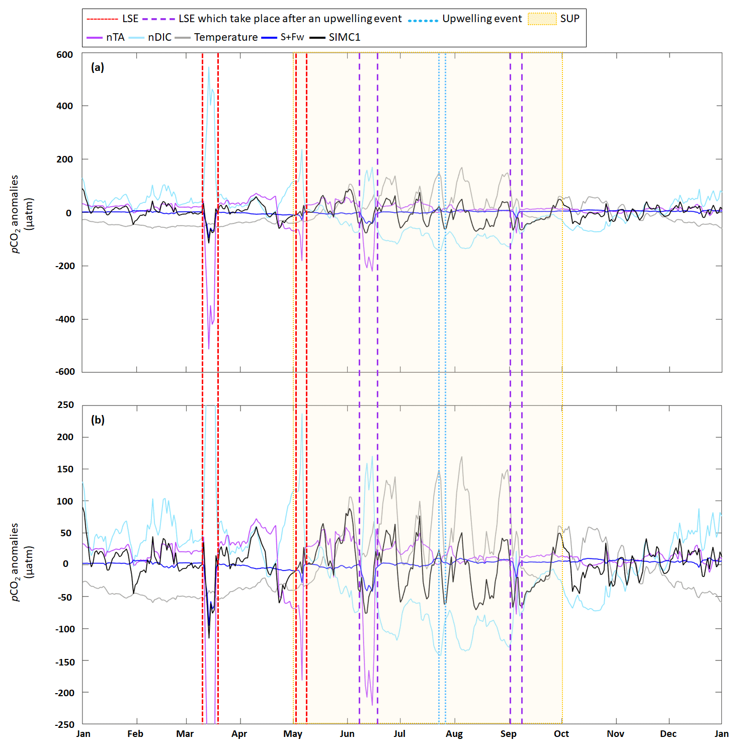
Figure D1 Time series for 2017 of daily average (a) pCO₂ anomalies generated by DIC, TA, S+Fw, and temperature based on the approach in Lovenduski et al. (2007) (note: the dark-blue line is sometimes obscured by the black line, especially in March); (b) enlargement of panel (a) between −250 and 250 µatm. LSE and an upwelling event have been highlighted. The summer upwelling period (SUP) is indicated by yellow shading.

Appendix E: DIC and nutrients – SOLEMIO data interpolation

As we represent a closed volume, we do not consider nutrients and DIC inputs which could be associated with LSEs or upwelling events (Gatti et al., 2006; Fraysse et al., 2013, 2014; Lajaunie-Salla et al., 2021). To assess if these inputs impact SOLEMIO, we interpolated DIC and nutrient measurements performed at the station, subsequently studying the trend observed during the events studied in the present study (Fig. E1).

Table E1 Surface DIC and nutrient concentration measurements at SOLEMIO station during LSEs and SUPs for the year 2017.

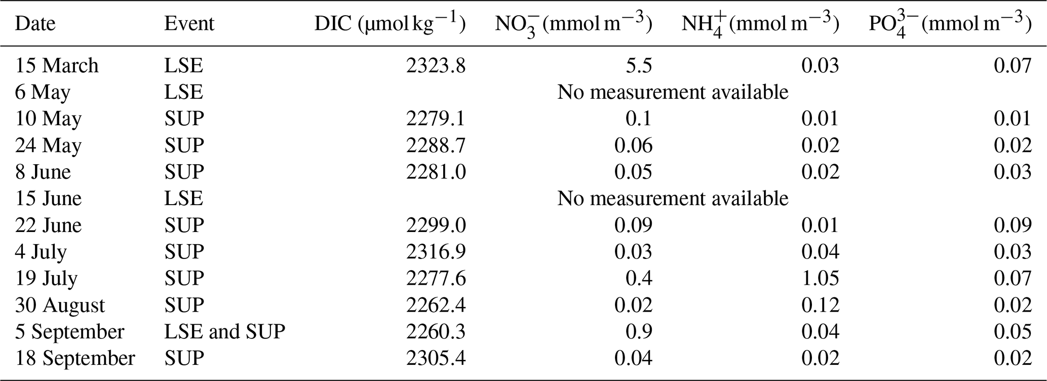
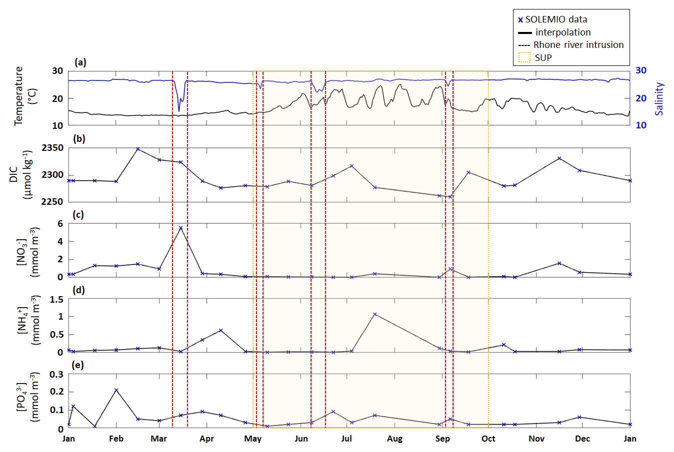
Figure E1 Time series of surface (a) temperature (PLANIER measurements, see Fig. 1 in Barré et al. (2023) for location) and salinity (CARRY measurements, see Fig.1 in Barré et al. (2023) for location) and interpolated (b) DIC, (c) NO${}_{\mathrm{3}}^{-}$, (d) NH${}_{\mathrm{4}}^{+}$, and (e) PO${}_{\mathrm{4}}^{\mathrm{3}-}$ concentrations at SOLEMIO station. SOLEMIO data are represented by blue markers. Rhône River intrusions studied here are indicated by the dotted red lines, and the SUP is shaded in yellow.

Appendix F: Sensibility analysis performed on air–sea CO₂ flux calculations

A sensibility analysis was performed to evaluate the importance of temperature, salinity, wind speed, and seawater–atmospheric pCO₂ difference terms in the air–sea CO₂ flux calculation. Previous terms are increased (decreased) one by one by 10 %. Air–sea CO₂ fluxes are then post-processed using Eqs. (8) and (9). The calculation is performed using MATLAB. We present in Table 4 the mean difference between the reference air–sea CO₂ fluxes (i.e., calculated without increasing (decreasing) one of the calculation terms by 10 %) and the air–sea CO₂ fluxes obtained by adding (removing) 10 % to (from) one of the terms of the calculation (Eq. F1).

$$\begin{array}{}\text{(F1)}& {\mathrm{\Delta }}_{\mathrm{Air}-\mathrm{sea}}{\mathrm{CO}}_{\mathrm{2}}\mathrm{Fluxes}={\displaystyle \frac{\mathrm{1}}{N}}\cdot {\sum }_{i=\mathrm{1}}^N\left(\text{abs}\left(\text{Ref}\right)-\text{abs}\left(X_{\mathrm{10}\mathit{\%}}\right)\right)\end{array}$$

In the above, Δ_Air−seaCO₂Fluxes is expressed in mmol m⁻² s⁻¹, and N is the number of modeled values. X represents temperature, salinity, wind speed, or the difference between seawater and atmospheric pCO₂.