Updating the radiation infrastructure in MESSy (based on MESSy version 2.55)

The calculation of the radiative transfer is a key component of global circulation models. In this article, we describe the most recent updates of the radiation infrastructure in the Modular Earth Submodel System (MESSy). These updates include the implementation of the PSrad radiation scheme within the RAD submodel. Furthermore, the radiation-related submodels CLOUDOPT (for the calculation of cloud optical properties) and AEROPT (for the calculation of aerosol optical properties) have been updated and are now more flexible in order to deal with different sets of shortwave and longwave bands of radiation schemes. In the wake of these updates, a new submodel (ALBEDO), which features solar-zenith-angle-dependent albedos and a new satellite-based background (white sky) albedo, was created. All of these developments are backward compatible, and previous features of the MESSy radiation infrastructure remain available. Moreover, these developments mark an important step in the use of the ECHAM/MESSy Atmospheric Chemistry (EMAC) model, as the update of the radiation scheme was a key aspect in the development of the sixth generation of the European Centre for Medium-Range Weather Forecasts – HAMburg (ECHAM6) model from ECHAM5. The developments presented here are also aimed towards using the MESSy infrastructure with the ICOsahedral Non-hydrostatic (ICON) model as a base model. The improved infrastructure will also aid in the implementation of additional radiation schemes once this should be needed.

We have optimized the set of free parameters for two general circulation model-type (GCM-type) setups for pre-industrial and present-day conditions: one with the radiation scheme that was used to date (i.e. the radiation scheme of ECHAM5) and one with the newly implemented PSrad radiation scheme. After this parameter optimization, we performed four model simulations and evaluated the corresponding model results using reanalysis and observational data. The most apparent improvements related to the updated radiation scheme are the reduced cold biases in the tropical upper troposphere and lower stratosphere and the extratropical lower stratosphere and a strengthened polar vortex. The former is also related to improved stratospheric humidity and its variability if the new radiation scheme is employed.

Using the multiple radiation call capability of MESSy, we have applied the two model configurations to calculate instantaneous and stratospheric-adjusted radiative forcings related to changes in greenhouse gases. Overall, we find that for many forcing experiments the simulations with the new radiation scheme show improved radiative forcing values. This is in particular the case for methane radiative forcings, which are considerably higher when assessed with the new radiation scheme and thus in better agreement with reference values.

1 Introduction

The most accurate models for calculating the radiative transfer within the atmosphere are line-by-line (LBL) models (e.g. Pincus et al., 2015). Results from radiative transfer calculations with these models agree well with observations (e.g. Oreopoulos and Mlawer, 2010; Oreopoulos et al., 2012; Pincus et al., 2015, and references therein). The shortwave (SW) and longwave (LW) broadband errors in the LBL models are of the order of 1 W m⁻² (Pincus et al., 2015, and references therein). However, these detailed radiative transfer models are computationally too expensive to be run in global climate models (e.g. Oreopoulos et al., 2012). Hence, in global climate models, the radiative transfer calculation is simplified compared to LBL models (e.g. Oreopoulos et al., 2012), and it is also, typically, not performed at every time step (Pincus and Stevens, 2013). Thus, there is the challenge for these simplified radiative transfer codes to be sufficiently precise and efficient (Pincus and Stevens, 2013). This causes the need to revise the radiation schemes which are employed in global models from time to time.

Here, we describe how we extended the Modular Earth Submodel System (MESSy; Jöckel et al., 2005, 2010) infrastructure to include the PSrad radiation scheme (Pincus and Stevens, 2013) for further use in MESSy-based climate simulations. The previous status of the MESSy radiation infrastructure is evident from Dietmüller et al. (2016). They document how the radiation infrastructure of the fifth generation European Centre for Medium-Range Weather Forecasts – HAMburg (ECHAM5; Roeckner et al., 2003, 2006) model was restructured to be “MESSy-fied”, i.e. to be modularized according to the MESSy coding standard: new (MESSy) submodels have been created from code parts of the radiation calculation which are related to, but to a certain degree independent of, the radiation scheme. These new submodels were (i) AEROPT, for the provision of aerosol optical properties; (ii) CLOUDOPT, for the calculation of cloud optical properties; and (iii) ORBIT, to determine the orbital parameters which are needed, for example, for the calculation of the radiative transfer. During this process, the structure of the radiation scheme was also MESSy-fied, and the corresponding MESSy submodel RAD was created.

Furthermore, Dietmüller et al. (2016) point out that the MESSy radiation infrastructure provides additional valuable features connected to the radiation calculation. One example is the possibility for multiple (diagnostic) calls of AEROPT, CLOUDOPT, and RAD, which can be used to determine multiple instantaneous radiative forcings (RFs) or stratospheric-adjusted RFs (as described by Stuber et al., 2001) online in a single simulation (see, e.g., Hansen et al., 2005, for a definition of instantaneous and adjusted RFs). This is a powerful feature, as the need for extensive output, which would be required for an offline (post-simulation) calculation, is avoided, and (if intended) all calculations are consistently performed with exactly the same version of the radiation scheme. Furthermore, the diagnostic calls are performed under the same meteorological conditions and at the highest possible frequency, i.e. the frequency of the radiation calls. Hence, a major concern during the development phase, which is described here, was to secure backward compatibility (up to the degree of binary identity to some point) and the possibility of retaining these features in connection with the newly added radiation scheme. Besides the integration of an additional radiation scheme, we also made the radiation infrastructure more flexible. Moreover, we created the MESSy submodel ALBEDO, which now contains the previous code for the calculation of the surface albedo extracted from the RAD submodel and newly added parameterizations for the calculation of the surface albedo.

As mentioned above, until now the default radiation scheme in MESSy was a modularized version of the ECHAM5 radiation scheme, which we will denote as E5rad throughout this paper. For many years, the Max Planck Institute for Meteorology (MPI-M) in Hamburg, Germany, has developed the general circulation model ECHAM (e.g. Roeckner et al., 1996, 2003; Stevens et al., 2013). An important step in upgrading the model from the fifth generation of ECHAM to ECHAM6.1 was an update concerning the radiation scheme, in particular as in the SW the number of bands was increased from 4 to 14 (Stevens et al., 2013). For the latest version of ECHAM, ECHAM6.3, the LW and SW radiation parameterization was revised once more, as the PSrad scheme (Pincus and Stevens, 2013) was made available (Giorgetta et al., 2018; Mauritsen et al., 2019). This version of ECHAM – with PSrad as the radiation model – also constitutes the atmospheric component of MPI-ESM1.2, the MPI-M's Earth System Model, which is described by Mauritsen et al. (2019). Simulations with MPI-ESM1.2 have contributed to the most recent phase of the coupled model intercomparison project (CMIP6; Eyring et al., 2016; see https://pcmdi.llnl.gov/CMIP6/ArchiveStatistics/esgf_data_holdings/, last access: 10 July 2023, for a list of available model output).

Similarly, PSrad is the radiation scheme employed in an ICOsahedral Non-hydrostatic (ICON was originally developed by the Deutscher Wetterdienst, DWD, and the MPI-M; Zängl et al., 2015) model version described by Giorgetta et al. (2018). We decided to add the PSrad scheme (as implemented in ICON version 2.4.0) to the radiation schemes, which are available within the MESSy infrastructure. This update marks an important step to incorporate previous model developments of the ECHAM family within the MESSy infrastructure, while it is also an important step towards the use of ICON as a base model within the MESSy infrastructure.

Furthermore, we expect a reduction in or removal of previous shortcomings related to the old radiation scheme when employing the new radiation scheme PSrad in ECHAM/MESSy Atmospheric Chemistry (EMAC) simulations. For example, previous studies with EMAC and the ECHAM5 radiation scheme have shown considerably low radiative effects for methane. For instance, a doubling of the present-day reference value for methane of 1.8 µmol mol⁻¹ resulted in a top-of-atmosphere stratospheric-adjusted RF of 0.23 W m⁻² (Winterstein et al., 2019; Stecher et al., 2021), while studies of Myhre et al. (1998) and Etminan et al. (2016) suggest 0.53 and 0.62 W m⁻², respectively, for the doubling of the reference value of 1.7 µmol mol⁻¹.

In the following, we present the recent developments concerning the radiation-related MESSy submodels, AEROPT, CLOUDOPT, and RAD, and the new MESSy submodel ALBEDO (Sect. 2). The general circulation model-type (GCM-type) atmosphere-only model setups (i.e. no interactive aerosol; only simplified methane chemistry) driven either by the new (PSrad) or the old (E5rad) radiation scheme, as well as the parameter optimization process, are presented in Sect. 3. This section also features the evaluation of these model setups with observational and reanalysis data. In Sect. 4, we show RF estimates derived using the old and new radiation scheme, and we compare our results to results from previous studies (Sect. 4). Finally, we close with a summary of the presented results (Sect. 5).

2 Radiation infrastructure updates

2.1 MESSy (short description)

Here, we describe the updates of the radiation infrastructure of the Modular Earth Submodel System (MESSy; Jöckel et al., 2005, 2010), which are now implemented in MESSy based on version 2.55. MESSy is a middleware to link different submodels (e.g. representing physical processes, chemical processes, online diagnostics, or external couplers) with a base (dynamical core) model. The key concept behind MESSy is that it provides the general infrastructure to perform simulations with a specific base model and clean interfaces, which allow the coupling of different submodels to this base model (Jöckel et al., 2005) or even the internal coupling of different modelling compartments (Pozzer et al., 2011). The software layers to ensure this clear separation are the base model layer (BML) and base model interface layer (BMIL), which contain the base model's code and the interface to connect submodels to the base model, respectively (Jöckel et al., 2005). Similarly, submodels are split into two layers which contain the core of the submodels computations in the submodel core layer (SMCL) and the submodel interface layer (SMIL) to connect with other submodels or the BMIL (Jöckel et al., 2005). The exchange of variables (between submodels, etc.) is handled via the “CHANNEL” interface (Jöckel et al., 2010) to avoid compile time dependencies between the core routines of different submodels.

Dietmüller et al. (2016) describe the state of the MESSy radiation infrastructure at the starting point of our new implementations. With the radiation infrastructure update and development of the submodels AEROPT, CLOUDOPT, RAD, and ORBIT, they took a big step towards a clean separation between (i) code components that are relevant for the radiation calculation but which can be separated, from a software development perspective, from the core radiative transfer model and (ii) the core radiative transfer model. Of course, it must still be ensured that the input and output variables of the submodels connect properly: for example, if the SW scheme has a set of bands, AEROPT and CLOUDOPT must provide aerosol and cloud optical properties for exactly those bands. Consequently, with the introduction of an additional radiation scheme, we had to update the submodels AEROPT and CLOUDOPT as the band structure of the newly added radiation scheme, PSrad, differs from the old one (see Sect. 2.2). Furthermore, we conducted an additional separation of the code that is independent of the core radiation calculation by creating the new MESSy submodel ALBEDO for the calculation of the surface albedo, which is then provided as an input for the radiation scheme. A key requirement of the updates was the preservation of previous flexibility, in particular concerning the application of multiple calls of the radiation scheme, as well as multiple calls of the aerosol and cloud optical schemes, as described by Dietmüller et al. (2016). Figure 1 gives an overview of the new radiation infrastructure. The following sections describe the updates for each of the radiation infrastructure submodels (i.e. all submodels that are directly related to calling the radiation scheme) in MESSy in comparison to the state described by Dietmüller et al. (2016). The described changes are available at the latest in ALBEDO version 1.4, AEROPT version 2.1.0, CLOUDOPT version 2.5, and RAD 3.0.

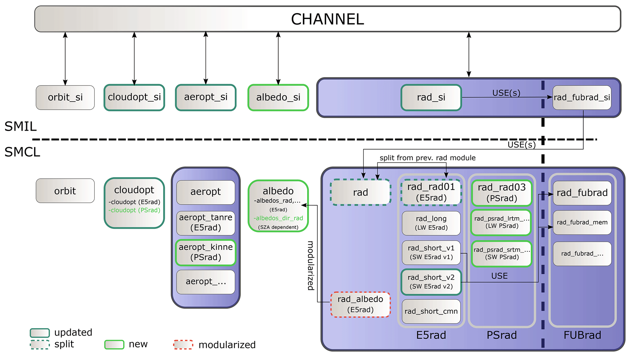
Figure 1 Schematic overview of the updated MESSy radiation infrastructure in comparison to the state described by Dietmüller et al. (2016, see also their Fig. 1). Green colour indicates new submodels (either Fortran modules or Fortran subroutines). Individual Fortran modules are shown as grey boxes. If the MESSy submodels encompass more than one Fortran module, then this is indicated via blueish boxes. See the text for details. In addition to the depicted changes, additional minor modifications, e.g. in the AEROPT core layer modules, have been made during the revision of the radiation infrastructure.

2.2 RAD: updates of the MESSy radiation submodel

The submodel RAD calculates the radiative transfer taking into account aerosols, clouds, and selected gaseous species relevant for radiative transfer (Dietmüller et al., 2016). Based on Dietmüller et al. (2016), we give the following recap of the RAD submodel before our implementation. In RAD, a MESSy-fied version of the ECHAM5 radiation scheme is available. This module comprises a LW radiation scheme with 16 bands (rapid radiative transfer model, RRTM; Mlawer et al., 1997) and two SW schemes (short_v1 and short_v2) with four bands each, both based on Fouquart and Bonnel (1980), whereas short_v2 includes the improvements of Thomas (2008). The MESSy submodel FUBrad (Nissen et al., 2007; Kunze et al., 2014) can be switched on to overcome the relatively coarse resolution in the SW, which allows for high-resolution UV radiative transfer calculations in the stratosphere above 70 hPa and extends the spectral range by including O₂ UV absorption in the Schumann–Runge bands/continuum and Lyman-α.

Here, we implemented the radiation scheme PSrad (Pincus and Stevens, 2013), as available in ICON version 2.4.0, into the MESSy submodel RAD. As described by Pincus and Stevens (2013), the development of PSrad was guided by RRTMG (rapid radiative transfer model for GCMs; Mlawer et al., 1997; Iacono et al., 2008). RRTMG in turn features 16 bands in the LW and 14 bands in the SW (Iacono et al., 2008; see also Tables 2.3 and 2.4 presented by Giorgetta et al., 2013, for the band structure). To make the PSrad scheme available alongside the “old” schemes, we introduce a new software “layer” in the MESSy RAD submodel core by splitting the previous core module “messy_rad.f90” into two new Fortran modules “messy_rad.f90” and “messy_rad_rad01.f90”, where the latter contains all subroutines from the previous “messy_rad.f90” directly related to the ECHAM5 radiation scheme(s). In analogy to “messy_rad_rad01.f90” for the old radiation scheme, “messy_rad_rad03.f90” provides the interface to the new radiation scheme (PSrad). The Fortran module was numbered with “rad03”, as in the SW rad01 already contains two schemes, rad_short_v1 and rad_short_v2. In principle, the two LW and three SW schemes can be combined freely, and the introduction of additional schemes should be straightforward if they are well modularized. However, for new combinations, additional parameter optimization (see Sect. 3.2) will likely be required. While it is still possible to use FUBrad with the old SW radiation schemes, this is not yet possible with the new SW scheme. In a future step, the new SW scheme is also envisaged to be available in combination with the FUBrad submodel. At the moment, however, the model terminates with a controlled shutdown and a corresponding error message if this combination is selected.

This implementation marks a major update of EMAC, as one key update between ECHAM5 and ECHAM6 was the update of the (SW) radiation scheme (Stevens et al., 2013), which in ECHAM6.3 was updated to PSrad (Giorgetta et al., 2018; Mauritsen et al., 2019). Furthermore, it also marks an important step for the transition towards ICON as a MESSy base model, as we implemented PSrad as available in the ICON version described by Giorgetta et al. (2018).

In addition to the distribution of greenhouse gases (GHGs) and meteorological data, the radiation scheme requires input regarding cloud optical properties, aerosol optical properties, and the surface albedo (see e.g. Dietmüller et al., 2016). For a typical simulation, this information now comes from the MESSy submodels CLOUDOPT, AEROPT, and the new submodel ALBEDO. Below, we describe, for such a typical simulation, how these radiation-related submodels (or previous Fortran routines in the case of ALBEDO) have been modified during the revision of the radiation infrastructure. However, we note that it is also possible to feed the respective input, e.g. from a previous simulation, into the RAD submodel via the MESSy submodel IMPORT (Kerkweg and Jöckel, 2015), which allows, among others, reading the time series of gridded data from NetCDF files.

2.3 AEROPT: updates of the MESSy submodel for the calculation of aerosol optical properties

The AEROPT submodel (Dietmüller et al., 2016) calculates the aerosol optical properties that are required for the radiative transfer calculation in the RAD submodel, namely aerosol optical depth for the LW and SW and single scattering albedo and asymmetry factor for the SW only, as scattering in the LW is considered neither in E5rad (Roeckner et al., 2003) nor in PSrad (Pincus and Stevens, 2013). These optical properties are wavelength-dependent. As the number of SW bands is different for PSrad compared to the old (ECHAM5) radiation scheme, the AEROPT submodel had to be revised. Consequently, the number of wavelength bands can vary between different sets of aerosol optical properties. We achieve this, as for each call the AEROPT submodel now provides CHANNEL objects with the corresponding number of wavelength bands.

Furthermore, the Max-Planck-Institute Aerosol Climatology version 1 (MAC-v1) for tropospheric aerosol optical properties described by Kinne et al. (2013) was made available via IMPORT and by introducing an ICON (version 2.4.0) routine (new MESSy Fortran module “messy_aeropt_kinne.f90”), which maps the aerosol optical properties to the model's current height profile and merges the climatologies for fine- and coarse-mode aerosol in the SW (see Giorgetta et al., 2013, for the mapping and merging details).

All other features of the AEROPT submodel, as described by Dietmüller et al. (2016), remain fully functional, e.g. multiple diagnostic calls of the AEROPT submodel or the combination of different aerosol sets. The latter is typically used to merge tropospheric and stratospheric aerosol data, and while merging, the consistency of the number of wavelength bands is checked. While it is still available for the old radiation scheme, the coupling of online-calculated aerosol is not yet implemented for the PSrad scheme. However, this functionality is due to be implemented with a revision of the AEROPT submodel.

2.4 CLOUDOPT: updates of the MESSy submodel for the calculation of cloud optical properties

The submodel CLOUDOPT (Dietmüller et al., 2016) provides the cloud optical properties which are needed for the calculation of the radiation in the submodel RAD. So far, in analogy to the aerosol optical properties provided by AEROPT, CLOUDOPT provides the band-dependent cloud optical properties of optical depth (again for LW and SW), single scattering albedo (SW), and the asymmetry factor (SW). We revised the CLOUDOPT submodel to account for the band structure of the new radiation scheme. CLOUDOPT now also contains the calculation of cloud optical properties as described by Stevens et al. (2013) and implemented in ICON (version 2.4.0). As for the AEROPT submodel, we generalized the infrastructure. Now, the number of wavelength bands of the CHANNEL objects can vary with each call of the CLOUDOPT submodel. Together with the adaptions in AEROPT, this allows us to call radiation schemes with different spectral resolutions within a single simulation for diagnostic purposes.

In the LW, the mass extinction coefficients of the new scheme follow the ECHAM5 parameterizations (Stevens et al., 2013) which were presented by Roeckner et al. (2003). For liquid clouds, the relation between effective radii and mass extinction is given in Eqs. (8) and (11.61) of Stevens et al. (2013) and Roeckner et al. (2003), respectively. For ice clouds, the parameterization is based on Ebert and Curry (1992, see Roeckner et al., 2003; Stevens et al., 2013). In addition, CLOUDOPT still allows the use of an alternative calculation for ice mass extinction in the LW, which was adopted from ECHAM4 (Eq. 101 and Table 3 of Roeckner et al., 1996). For the SW, the new scheme derives the mass extinction, single scattering albedo, and asymmetry factors from lookup tables (Stevens et al., 2013), whereas the old scheme uses a set of coefficients to derive SW optical properties from effective radii (Roeckner et al., 2003).

As in ECHAM5 and ECHAM6, the cloud optical depths of liquid and ice clouds are rescaled using a cloud inhomogeneity factor to account for the subgrid-scale variability of the clouds (Roeckner et al., 2003; Mauritsen et al., 2012; Stevens et al., 2013; Mauritsen et al., 2019; Mauritsen and Roeckner, 2020; see keywords “zinhoml” and “zinhomi” in the supporting information of the latter). For liquid clouds, the inhomogeneity factors can now be set, depending on the cloud type (convection type). In the namelist, three inhomogeneity factors can be set for convection-free, convective, and certain shallow convective clouds (see Mauritsen et al., 2019; Mauritsen and Roeckner, 2020, and the supporting information of the latter) in analogy to the implementation in ECHAM6.3 and ICON.

In CLOUDOPT and in the radiation schemes, the (default) cloud overlap is assumed to be maximum random overlap (Roeckner et al., 2003; Dietmüller et al., 2016; Giorgetta et al., 2018). In the case of PSrad, the overlap assumption is treated based on the Monte Carlo Independent Column Approximation (McICA) technique (see Giorgetta et al., 2018, for details and further references).

2.5 ALBEDO: introduction of the new MESSy submodel for the calculation of surface albedos

As a final step to separate the code from the RAD submodel that is independent of the radiation scheme, the calculation of the surface albedo was modularized. Therefore, we introduced the new submodel ALBEDO. This new MESSy submodel contains the previous (ECHAM5-based) routines to calculate the surface albedo and was extended by adding new parameterizations and additional features for the calculation of solar-zenith-angle (SZA)-dependent surface albedos. In particular, ALBEDO calculates a blue sky albedo (α_blue) from the black sky (α_black) and white sky albedo (α_white) and the fraction of direct and diffuse radiation fluxes with respect to the total downwelling shortwave fluxes at the surface ($f_{\mathrm{sw},\mathrm{surf}}^{\mathrm{dir}}$, $f_{\mathrm{sw},\mathrm{surf}}^{\mathrm{dif}}$) as ${\mathit{\alpha }}_{\mathrm{blue}}=f_{\mathrm{sw},\mathrm{surf}}^{\mathrm{dir}}{\mathit{\alpha }}_{\mathrm{black}}+f_{\mathrm{sw},\mathrm{surf}}^{\mathrm{dif}}{\mathit{\alpha }}_{\mathrm{white}}$ (see, e.g., Liu et al., 2009; Li et al., 2018; Cordero et al., 2021, and references therein for details on the different albedos and how to typically derive the blue sky albedo). Here, the black sky albedo relates to the albedo associated with the collimated beam, whereas the white sky albedo corresponds to the albedo associated with isotropic diffuse radiation (Liu et al., 2009). Further details on the modularization and updates are described below.

2.5.1 ECHAM5 (background) albedo

ECHAM5 uses a so-called background albedo for snow-free land surfaces (Roeckner et al., 2003). This temporally constant (i.e. without interannual or subseasonal variation) climatological field is based on Hagemann (2002). This background albedo is modified according to meteorological and land properties, and an albedo for grid points containing sea ice is calculated (Roeckner et al., 2003). Finally, the resulting fields are combined with a constant value for the albedo of ice-free ocean surfaces to produce the final (blue sky) albedo employed in the ECHAM5 model (Roeckner et al., 2003). The corresponding routine is shifted to the core layer of the new ALBEDO submodel and is called from the respective submodel interface layer.

2.5.2 New white sky albedo for snow-free land

Here, we introduce a new white sky albedo for snow-free land surfaces, which can be used to calculate SZA-dependent surface albedos and is practically a substitute for the previous ECHAM5 background albedo. This white sky albedo is a monthly mean climatology based on data from the Moderate Resolution Imaging Spectroradiometer (MODIS; https://modis.gsfc.nasa.gov/about/, last access: 3 February 2023). Furthermore, in principle, it is possible to use any (background or white sky) albedo with any temporal resolution as input via IMPORT, since the (background or white sky) albedo is now namelist-controlled. So, besides the newly added monthly climatology with subseasonal variation, other albedo data with different variability (e.g. transient) could also be fed in as background albedo via IMPORT.

The provided white sky albedo was produced from the MODIS/Terra+Aqua BRDF/Albedo Gap-Filled Snow-Free Daily L3 Global 30ArcSec CMG V006 data product (MCD43GFv006; Sun et al., 2017; Schaaf, 2019). We used the white sky albedo near-shortwave broadband and the period from 1 January 2001 to 31 December 2010. The original data are daily files on a 43 200 × 21 600 grid. This grid corresponds roughly to a pixel size of 1 km × 1 km. Values of the white sky albedo below 0.07 in the raw daily files are set to missing (guided by the reference value for the ocean surface albedo used in ECHAM5; Roeckner et al., 2003), and the resulting files are further used to calculate monthly means. We calculate a climatology over all months, which we use to fill in missing values in the original monthly mean files; i.e. we substitute missing values in the original monthly files with a climatological value calculated from the original monthly files where the particular pixel is not missing. Consequently, a 12-month climatology is calculated from the collection of the updated monthly files. The all-time climatology is used to create common generic conversion weights to remap both climatologies (all time and 12 months) to a 360×180 grid. Any remaining missing grid points in the two climatological files – which can occur, as there might be grid points which are missing in all months which were used to calculate the climatology – are filled using a nearest-neighbour method. This procedure ensures that when the resolution-dependent land mask is applied in a simulation, the white sky albedo for snow-free land includes land albedo values only.

2.5.3 Solar-zenith-angle-dependent albedo

One main aspect during the modularization of the ALBEDO submodel was to include the SZA dependence of the albedo for water, land, and snow. For the SZA dependence of the ocean surface, the parameterization, as described in Appendix A of Li et al. (2006), was implemented (with a scaling factor to achieve improved global mean SW fluxes; see Sect. 3.2). Li et al. (2006) refer to this parameterization as being based on the Preisendorfer and Mobley (1986) scheme. The SZA-dependent land surface albedo is parameterized depending on the surface properties, as in Appendix B of Briegleb (1992), which is analogous to the implementation in the ICON module mo_albedo.f90. For the snow albedo, we use the parameterization as given in Formula A3 of Yang et al. (2001; see also Appendix B of Briegleb, 1992, and references therein).

When the SZA dependence is used, the procedure to calculate the blue sky albedos is as follows. The white sky albedo, e.g. from MODIS (see above), is modified according to meteorological properties and land properties, as well as ice cover (as was the ECHAM5 background albedo before), and an albedo for sea ice is calculated (again, as in ECHAM5). Based on this white sky albedo and the respective parameterizations (see the previous paragraph), a SZA-dependent black sky albedo for land (snow-covered and snow-free) and ice-covered (snow-covered and snow-free) surfaces is calculated. Additionally, over (ice-free) ocean surfaces, a white sky and black sky albedo is calculated based on the wind speed and the SZA (Yang et al., 2001). From these white sky and black sky albedos and the diffuse and direct SW surface radiation fluxes, the blue sky albedo is obtained.

To be able to use this new feature, either the radiation scheme has to provide (the fraction of) the direct and diffuse SW radiation fluxes from the previous model time step (at the first model time step, the partitioning is automatically set to 0.9 and 0.1, respectively), or the user has to set a fixed relation between these fluxes via a namelist. The former is the case for both PSrad and the SW scheme rad_short_v2, which was slightly adapted to this end, whereas the latter is the case for rad_short_v1.

2.6 Minor modifications of the radiation infrastructure

During the restructuring of the radiation infrastructure, we made several minor adjustments in addition:

1. ECHAM5 commonly performs (full) radiation calls less frequently than at each model time step (Roeckner et al., 2003). Thus, the output from a specific radiation call is used at several model time steps. Hence, at a time step at which a new (full) radiation call is performed, the orbital parameters are advanced (by Δt_orb) for the radiation call (Roeckner et al., 2003). The results from this radiation call (with the adjusted orbital parameters) are later on corrected with the solar irradiation associated with the orbital parameters of the actual model time step for the calculation of the actual SW fluxes and heating rates (see Roeckner et al., 2003). We note that the adjusted SZA contains a modification which ensures that fluxes are non-zero globally to avoid problems in the grid boxes in which the Sun rises or sets during the time steps associated with the radiation time step (see Roeckner et al., 2003; also see their Eq. 11.23). Figure 2 illustrates the alignment of model time steps and radiation calls, where the colours highlight which model time steps are associated with a specific full radiation call. Previously, the orbital parameters were shifted to the middle of the interval between the current and the next full radiation call, including the latter (Fig. 2a). We think that this choice is inconsistent, as the results from the full radiation calculation are corrected later on with the exact orbital parameters of the time steps associated with the full radiation call. As a consequence, the offset orbital parameters should be as close as possible to the actual orbital parameters which are later used for the correction. Hence, the orbital parameters should be shifted to the middle of the interval of the time steps associated with the current radiation call ($t_{\mathrm{r},i-\mathrm{1}}$, $t_{\mathrm{r},i-\mathrm{1}}+\mathrm{\Delta }{t}_{\mathrm{m}}$,…, $t_{\mathrm{r},i}-\mathrm{\Delta }{t}_{\mathrm{m}}$, which leads to $\mathrm{\Delta }{t}_{\mathrm{orb},\mathrm{opt}\mathrm{1}}=\frac{\mathrm{1}}{\mathrm{2}}\left(\right(t_{\mathrm{r},i}-\mathrm{\Delta }{t}_{\mathrm{m}})-t_{\mathrm{r},i-\mathrm{1}})$; Fig. 2b). Besides this choice of the offset, which is our new default, the offset type can be set via a new namelist switch, and there is the option to use the old default Δt_orb,opt0 to ensure backward compatibility, or the offset can be set to an arbitrary constant ($\mathrm{\Delta }{t}_{\mathrm{orb},\mathrm{con}}\le \mathrm{\Delta }{t}_{\mathrm{r}}$). The latter option was introduced for offline radiation calculations.

2. The so-called diffusivity factor (see, e.g., Roeckner et al., 2003; Li, 2000, and references in the latter), which is used to scale the optical thickness of the clouds in the LW, was removed from the CLOUDOPT submodel and is now accounted for (exactly once) in the radiation schemes to avoid any confusion. Originally, the application of the diffusivity factor was partly mixed into the parameters that were used to calculate LW cloud optical thicknesses and partly applied later in the code for the new radiation scheme, while it was accounted for in the cloud optical properties for the old scheme. This restructuring caused changes in the output of CLOUDOPT and the binary divergence of model results based on the old and the new code when applying the old (ECHAM5) radiation scheme.

3. The distance between Sun and Earth (zdisse) was updated to account for the shift of the orbital parameters by Δt_orb. Although this change is expected to have a negligible impact on the model results, we note it here, as it destroys the binary identity.

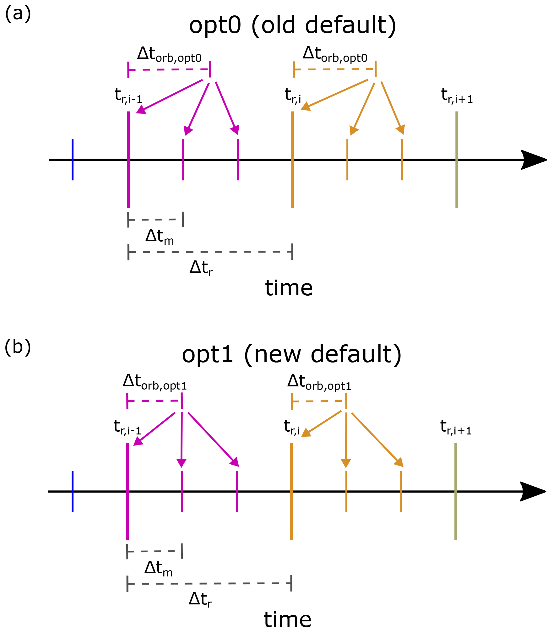
Figure 2 Schematic of the radiation calls for three model time steps per full radiation call (long vertical lines, e.g. t_r,i) for the old (a) and new (b) choice of the offset parameter (Δt_orb). For Δt_m<Δt_r (no full radiation calculation at every model time step), previously (a) the orbital parameters were shifted according to $\mathrm{\Delta }{t}_{\mathrm{orb},\mathrm{opt}\mathrm{0}}=\frac{\mathrm{1}}{\mathrm{2}}(t_{\mathrm{r},i}-t_{\mathrm{r},i-\mathrm{1}})$, whereas the new option shifts the parameter according to $\mathrm{\Delta }{t}_{\mathrm{orb},\mathrm{opt}\mathrm{1}}=\frac{\mathrm{1}}{\mathrm{2}}\left(\right(t_{\mathrm{r},i}-\mathrm{\Delta }{t}_{\mathrm{m}})-t_{\mathrm{r},i-\mathrm{1}})$. In addition to the old and new choice of the offset parameter (Δt_orb), it is now also possible to set this parameter via a namelist to a constant ($\mathrm{\Delta }{t}_{\mathrm{orb},\mathrm{con}}\le \mathrm{\Delta }{t}_{\mathrm{r}}$).

2.7 Overview of the new radiation infrastructure dependencies

The interplay of the radiation-related submodels is presented as a schematic in Fig. 3 for a typical (new) setup. Red arrows mark the two new dependencies that now exist: (1) the direct and diffuse surface fluxes from the last radiation update (box with “rad upd.” in Fig. 3) are provided to the ALBEDO submodel. (2) The orbital parameters (most importantly the SZA) are calculated by ORBIT and provided to the ALBEDO submodel, which then calculates the albedo for the next full radiation calculation. We note that the latter dependency was hidden before, as the calculation of the surface albedo was performed in the RAD submodel. While the other dependencies (black arrows) already existed before our developments, all submodels (RAD, ALBEDO, CLOUDOPT, and AEROPT), except for ORBIT, have been revised and are more flexible now.

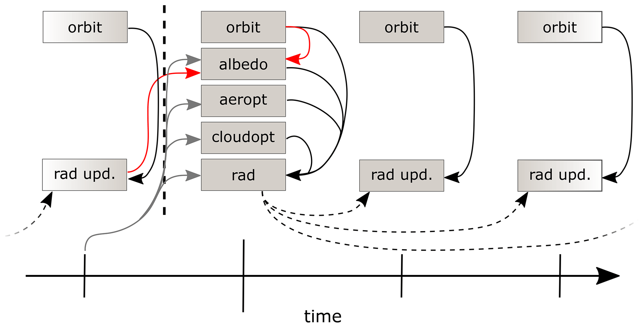
Figure 3 Schematic of the interdependencies of the radiation infrastructure for a typical simulation setup with the new radiation scheme. Grey arrows show information (e.g. temperature and pressure) from the model time step (vertical bars) before a full radiation time step (long vertical bar) that is passed into radiation-related submodels. In a full radiation step (long vertical bar), the radiative transfer is calculated and stored based on an offset of the orbital parameters. Dashed arrows show that information from a full radiation time step is forwarded to the radiation update (rad upd.) time steps. At these time steps for the SW, updates of the radiative fluxes and heating rates are calculated and applied (see Roeckner et al., 2003). This correction is also applied during full radiation calls (see Sect. 2.6). Red arrows show new dependencies. Input from the previous radiation update (fluxes at surface) and the information from ORBIT (mainly SZA) are fed to the ALBEDO submodel.

The processing chain of the radiation calculation is as follows. At a full radiation time step (long vertical bar in Fig. 3), the information (e.g. temperature, pressure, cloud, aerosol, and gases) from the previous model time step is available to ALBEDO, AEROPT, CLOUDOPT, and RAD. Additionally, fluxes from the last radiation update are available for the ALBEDO submodel, which also receives information from ORBIT, in particular the SZA. Then, the different radiation-related submodels are called and pass their information to RAD. Finally, the full radiation calculation is performed with an offset of the orbital parameters, and the results are stored. The SW fluxes at the model time steps are then calculated via a simple update of the radiation fluxes (as in ECHAM5; see Roeckner et al., 2003). Note that “rad upd.” is also performed for the full radiation time step, as the orbital parameters used for the radiative transfer are typically shifted in comparison to the orbital parameters (mainly SZA) associated with the current model time step (see Δt_orb Sect. 2.6).

3 Evaluation of the new (GCM-type) configuration

During the implementation of the presented updates, it was ensured that previous model results could be reproduced after the restructuring of the code. In particular, binary identity was secured up to a point where required changes (see Sect. 2.6; e.g. “diffusivity factor”) break binary identity. A key strength of the MESSy concept is that many (including previous) model configurations can be run with the same executable by adjusting the Fortran namelists only. Accordingly, the four simulations discussed hereafter can be performed with the same executable by changing three namelist files (RAD, ALBEDO, and IMPORT) only. As we have performed diagnostic radiation calls with an exchanged radiation scheme (e.g. driving the simulation with PSrad and performing an additional diagnostic radiation call with E5rad; see Sect. 4), the CLOUDOPT and AEROPT namelist files already included the calculation of aerosol and cloud optical properties for both (E5rad and PSrad) radiation schemes. Hence, these namelist files did not have to be adjusted when the driving radiation scheme was switched.

3.1 Simulation setups

We performed four simulations for the evaluation presented here, namely two simulations (pre-industrial and present-day denoted with pi and pd, respectively) for each of the two radiation schemes (the old ECHAM5 radiation scheme with the v2 in the SW, denoted here with E5rad, and the newly implemented PSrad scheme). These simulations will be addressed here as EMAC-E5rad-pi, EMAC-E5rad-pd, EMAC-PSrad-pi, and EMAC-PSrad-pd, respectively. The simulation setups do not only differ in terms of the radiation scheme but also, according to the respective radiation scheme, the typical old and new setups of AEROPT, CLOUDOPT, and ALBEDO (as described before) have been chosen, as indicated in Table 1. In all simulations, the new choice for the orbital offset parameter (Δt_orb) was employed.

The simulations were conducted with T42 spectral truncation (corresponding to about 2.8° × 2.8°; i.e. roughly 300 km × 300 km at the Equator) and 90 vertical levels extending up to roughly 80 km (see the T42L90MA setup as, e.g., mentioned by Jöckel et al., 2016). The model time step length was set to 600 s, and full radiation calculations were performed at every third model time step.

For the solar forcing, we applied a total solar irradiance (TSI) of 1360.75 W m⁻², representing approximately the average TSI of the first 2 decades (first two solar cycles) in the time series displayed in Fig. 1 of Matthes et al. (2017a, b; data are also available from https://solarisheppa.geomar.de/cmip6, last access: 28 May 2024), i.e. representing pre-industrial conditions. Although Fig. 1 of Matthes et al. (2017a) indicates an increase in TSI from the pre-industrial conditions to the end of the 20th century (to roughly 1361.25 W m⁻²), we have kept the TSI constant for the present-day simulations. The increase of about 0.5 W m⁻², is not of substantial relevance in the global energy budget of Earth, as only one-quarter of this difference remains for Earth's global average, which is further reduced as a part of this additional solar irradiance is reflected. Thus, we expect the change from pre-industrial to present-day conditions to be of the order of about 0.1 W m⁻² in the end.

Table 1 presents additional forcings and boundary conditions. These represent pre-industrial (pi, representative of the year 1850 conditions with some deviations due to data availability) and present-day conditions (pd, representative of the year 2000 conditions). A short outline of the employed boundary data is given below.

The four simulations use prescribed sea surface temperatures (SSTs) and sea ice cover (SIC; Rayner et al., 2003), and the quasi-biennial oscillation (QBO) is nudged, as described by Jöckel et al. (2016). Except for simplified methane chemistry, these simulations feature no chemistry and are thus described here as GCM-type simulations as opposed to chemistry–climate model simulations. In the lowest model level, methane (CH₄) is nudged to surface mixing ratios according to historical CMIP6 data (Meinshausen et al., 2017). In the atmosphere, the simplified methane chemistry includes two effects: (i) the methane oxidation, which is represented by the MESSy submodel CH₄ (Winterstein and Jöckel, 2021) using prescribed climatologies of the methane reactions partners (OH, O(¹D), and Cl) from previous EMAC simulations, namely EMAC-DECK-piControl and EMAC-RD1-base-01 (Jöckel, 2023; see also https://data.ceda.ac.uk/badc/ccmi/data/post-cmip6/ccmi-2022/DLR/EMAC-CCMI2/refD1, last access: 28 May 2024), which were conducted according to the CMIP6 (Eyring et al., 2016) and CCMI-2 (https://blogs.reading.ac.uk/ccmi/ccmi-phase-two/, last access: 17 July 2023; for phase one of CCMI, see Eyring et al., 2013; Morgenstern et al., 2017) protocols, respectively. Water vapour tendencies due to methane oxidation are consequently accounted for in the interactive water vapour field of the simulation. (ii) Methane is photolysed using a photolysis rate which is calculated online by the MESSy submodel JVAL (Sander et al., 2014). The corresponding water vapour and methane fields are used in the first call of the radiation module and thus are driving the simulation.

All other trace gas fields required by the radiation schemes, e.g. carbon dioxide (CO₂), nitrous oxide (N₂O), ozone (O₃), and the chlorofluorocarbons CFC-11 and CFC-12, also stem from comprehensive chemistry–climate model simulations which were previously conducted with EMAC, namely EMAC-DECK-piControl and EMAC-RD1-base-01. Additional diagnostic radiation calls were performed with the imported methane fields from these previous EMAC simulations.

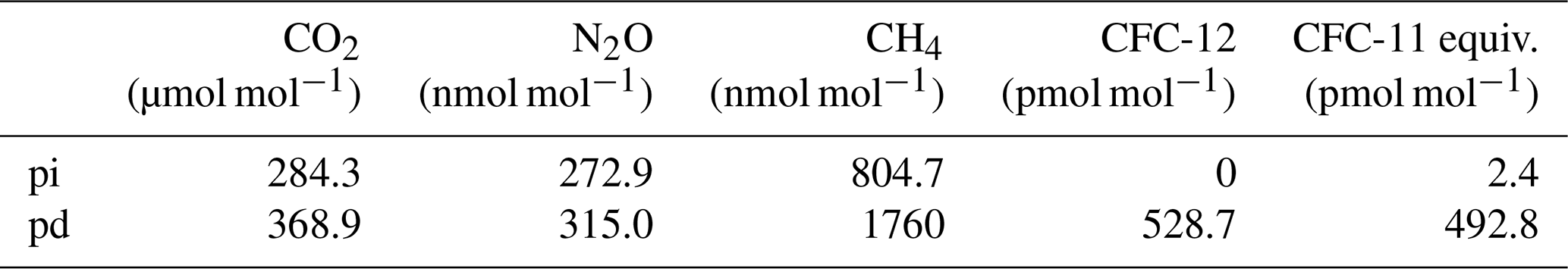
The CO₂, CH₄, and N₂O fields of these previous simulations in turn are based on the respective historical CMIP6 data presented by Meinshausen et al. (2017), which are used as lower boundary conditions in these simulations. Table 2 presents the climatological surface level mixing ratios of these simulations. These values are in agreement with the values presented in Table 5 of Meinshausen et al. (2017) for 1850 and 2000 conditions.

(Rayner et al., 2003)(Naujokat, 1986)Meinshausen and Vogel (2016)Meinshausen et al. (2017)ETH Zürich (2017)Tanre et al. (1984)Hagemann (2002)Roeckner et al., 2003(Roeckner et al., 2003)Kinne et al. (2013)(Sun et al., 2017; Schaaf, 2019)Roeckner et al., 2003(Stevens et al., 2013)

Table 1 Boundary conditions of the simulations for pre-industrial and present-day conditions with radiation scheme E5rad and PSrad. Monthly mean data are abbreviated as mm. Please see the text for details.

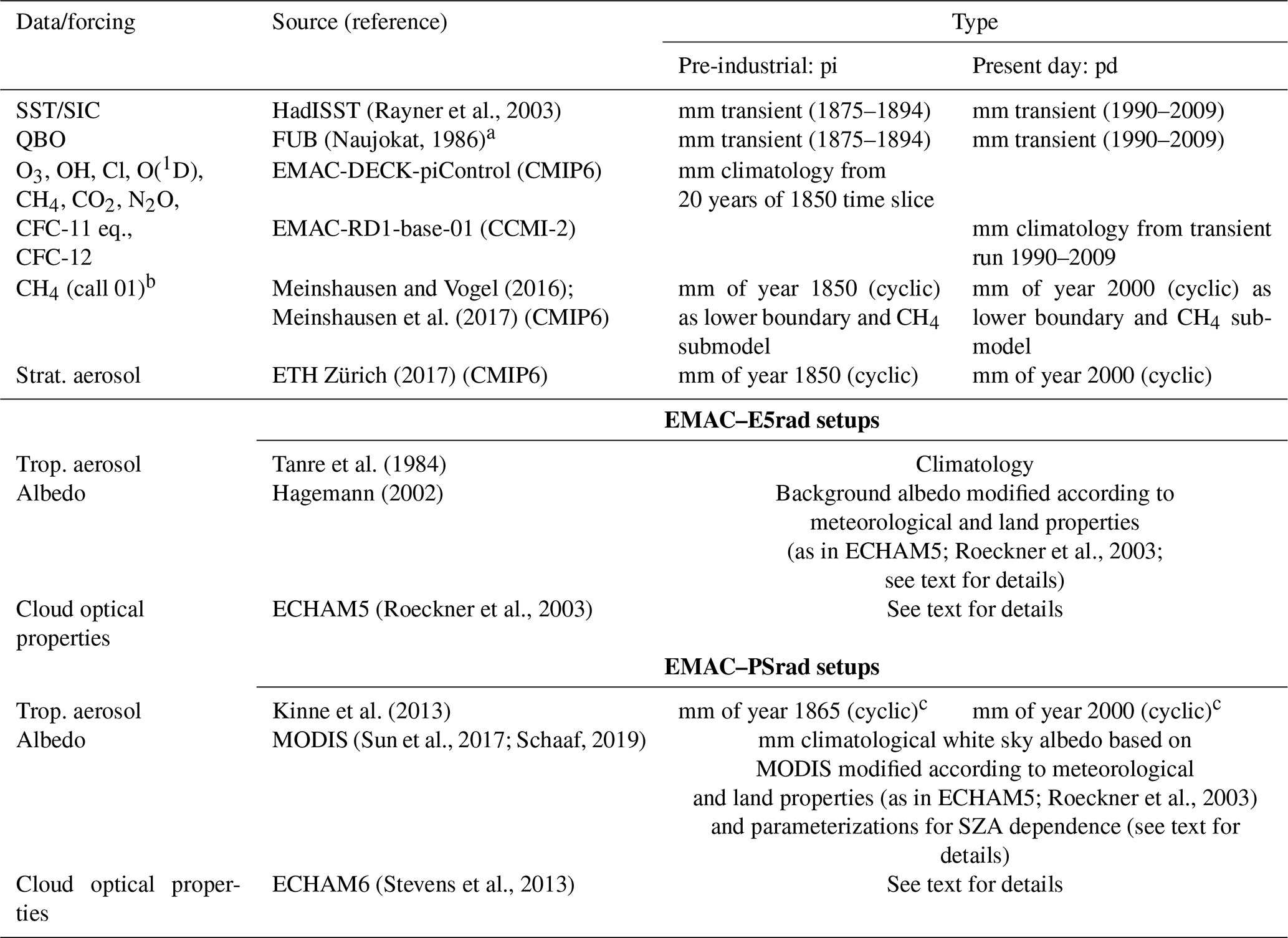
^a For the QBO, an extension method (see https://www.pa.op.dlr.de/CCMVal/Forcings/qbo_data_ccmval/u_profile_195301-200412.html for a description, last access: 19 July 2023) was applied to observational data available from the FUB (Freie Universität Berlin; https://www.geo.fu-berlin.de/en/met/ag/strat/produkte/qbo/index.html, last access: 19 July 2023; see also Naujokat, 1986). ^b Lower boundary conditions and simplified methane chemistry were used to produce the CH₄ field which drives the simulations. However, for additional radiation calls, the CH₄ from previous EMAC simulations, as for other GHGs, is being used to ensure that the CH₄ fields are identical in the simulation driven with E5rad and PSrad and that they match with the other GHGs. ^c The aerosol data set by Kinne et al. (2013) is a mm climatology for the coarse aerosol, whereas the fine-mode aerosol is mm transient (see also Giorgetta et al., 2013).

For CFC-12, the global mean values in the lowest model level are 0 and 528.7 pmol mol⁻¹ for pi and pd conditions, respectively (see Table 2). These values are in agreement with the lower boundary values they are based on, which were presented by Meinshausen et al. (2017) and Carpenter et al. (2018). To include the effect of additional radiatively active ozone-depleting substances (ODSs), the approach outlined by Meinshausen et al. (2017) to lump additional radiatively active ODSs via radiative efficiencies (see e.g. Burkholder, 2018) to CFC-11 equivalents for purposes of radiative transfer calculations was applied in the EMAC-DECK-piControl and the EMAC-RD1-base-01 simulations. For the EMAC-DECK-piControl, eight species have been lumped to CFC-11 equivalents, based on values presented by Meinshausen et al. (2017), whereas for the EMAC-RD1-base-01 only six species have been lumped according to the data given by Carpenter et al. (2018). This results in global mean values of 2.4 and 492.8 pmol mol⁻¹ of CFC-11 equivalents in the lowest level of the EMAC-DECK-piControl and EMAC-RD1-base-01 simulation, respectively. This is lower than the expected full CFC-11 equivalents for the respective periods, which are of the order of 30 pmol mol⁻¹ for pre-industrial conditions and above 700 pmol mol⁻¹ for the 2000s (see Meinshausen et al., 2017). However, the lower CFC-11 equivalent mixing ratios in the EMAC simulations are in agreement with the respective reference values, given the reduced number of accounted (lumped) species in the model setups.

In all simulations, stratospheric aerosol data from ETH Zürich (2017), as proposed for CMIP6, were employed. The tropospheric aerosol data are based on Tanre et al. (1984) and Kinne et al. (2013) for E5rad (as described by Roeckner et al., 2003, for ECHAM5) and PSrad, respectively. Concerning the surface albedo, the E5rad simulations use the previous ECHAM5 routines to adapt the ECHAM5 background albedo (for details, see Hagemann, 2002; Roeckner et al., 2003), whereas the PSrad simulations use the surface albedo computed with the newly implemented solar-zenith-angle-dependent albedo (for water, land, and snow), where the white sky albedo for snow-free land was derived from MODIS (see Sect. 2.5). Hence, except for tropospheric aerosol data and the albedo, the boundary conditions for the E5rad and PSrad simulations were identical.

After optimizing the set of free parameters of the model with respect to the boundary data and the respective radiation scheme (see the description in Sect. 3.2), the simulations were performed for 20 years, while our analyses exploit only the last 10 years of each of the simulations to reduce the risk of any possible influence from the spin-up period. To reduce the amount of data, model output was aggregated as monthly mean values on model levels. These monthly means were calculated online (i.e. all model time steps are accounted for in the means), and whenever necessary, they were interpolated to pressure levels offline.

Without additional diagnostic radiation calls for RF calculations, as presented in Sect. 4, for a simulation performed on a single node¹, the computational time required for a radiation time step is around 70 % higher for the PSrad setups than for the E5rad setups. If the full radiation calls are only performed at every third time step (as in the simulation setups described above), then this leads to an increase in the computational time of roughly 40 %. This increase in computational time cannot be solely attributed to the core radiative transfer routines in RAD but is also affected by possible changes in computational time in the connected submodels AEROPT, CLOUDOPT, and ALBEDO. To put this increase into perspective, we note that EMAC is commonly used in setups with comprehensive interactive chemistry (e.g. as a chemistry–climate model). Due to the large computational demand of the chemistry solver, the increase in computational time due to the radiation scheme will only be a fraction of the increase we report here for a GCM-type setup.

Table 2 Global mean surface level (lowest model level) mixing ratios as employed in the pi and pd simulations based on fields from the previous EMAC simulations, EMAC-DECK-piControl and EMAC-RD1-base-01.

3.2 Parameter optimization for the GCM-type setups

Earth receives approximately 0.34 kW m⁻² of solar radiation at the top of the atmosphere (TOA) on average, which is almost balanced by TOA reflected SW radiation (∼ 0.1 kW m⁻²) and TOA outgoing LW radiation (∼ 0.24 kW m⁻²; e.g. Trenberth et al., 2009; Stephens et al., 2012; Wild et al., 2015). It is challenging to assess the resulting imbalance (Johnson et al., 2016), which is somewhat below 1 W m⁻² (e.g. Trenberth et al., 2009; Wild et al., 2015, and Johnson et al., 2016 present estimates within 0.6–0.9 W m⁻²). The best estimates are derived from heat uptake analyses (Johnson et al., 2016) which are used to calibrate satellite-based observations (Loeb et al., 2009, 2018).

Similarly, in global (climate) models, the TOA (im)balance is commonly “calibrated” to observed estimates during the so-called tuning process (Hourdin et al., 2017). Here, we optimize the four setups that are described in the section above (Sect. 3.1). Our two primary targets were (i) a radiative balance at TOA close to 0 W m⁻² for the pre-industrial configuration (assuming that during that period the Earth's energy budget was almost balanced) and (ii) a radiative imbalance at TOA around 1 W m⁻² for the present-day configuration with the same parameter set (accounting for the expected imbalance; see above). Furthermore, we aimed for clear- and all-sky LW and SW present-day TOA radiation fluxes to be within the uncertainty range of satellite-based observational estimates (Loeb et al., 2018; CERES Science Team, 2021) while securing the hydrological cycle to remain within an acceptable range compared to observations (see below). For a more elaborate review of the principles of climate model tuning, which we will address also as parameter optimization in the following, we refer the reader to Mauritsen et al. (2012).

To achieve our goals, we adjusted parameters associated with clouds, convection, and the surface albedo while keeping the previous defaults, e.g., for parameters related to the parameterization of gravity waves. Table 3 lists the final parameter set along with previously used parameter values. Prior knowledge of sensitivities of the radiative fluxes regarding typical optimization parameters from Mauritsen et al. (2012, Fig. 3) and Kern (2013, Appendix D) allowed us to adjust parameters in a target-oriented manner without extensive testing of all possible sensitivities.

As a starting point for the model optimization, we used typical ECHAM6.3 values for the inhomogeneity factors for liquid and ice clouds (Mauritsen et al., 2019). All other optimization parameters were set to the previous EMAC defaults. First, we targeted the TOA global annual mean clear-sky SW fluxes via the surface albedo as there is no (substantial) dependence of these fluxes on the other optimization parameters. During this process, we increased the minimum albedo of bare sea ice from 0.50 (see Roeckner et al., 2003) to 0.55 (a value that has been previously used in other EMAC simulation setups) and increased the ocean surface albedo by a factor of 1.15 to enhance the outgoing SW clear-sky radiation at TOA to roughly match satellite-based estimates (Loeb et al., 2018). Second, we targeted the TOA LW flux by increasing a parameter that influences a geopotential-based conversion rate from cloud water to rain in convective clouds (cprcon) to the value used for ECHAM6.3 in T63 spectral resolution (Müller et al., 2018). Third, targeting the TOA SW flux, which is sensitive to various parameters (see, e.g., Mauritsen et al., 2012), we decreased the convective mass flux above the level of non-buoyancy (cmfctop) to 0.23, which now lies between the previous EMAC default and the value used in ECHAM6.3 in T63 spectral resolution (Müller et al., 2018).

(Mauritsen et al., 2019)(Mauritsen et al., 2019)(Müller et al., 2018)(Müller et al., 2018)(Roeckner et al., 2003)

Table 3 Comparison of optimized parameters for the final simulation setups with previously used values. Note that the parameter values for the newly optimized simulations (middle column) are within an acceptable range of previously used parameter sets for ECHAM (right column).

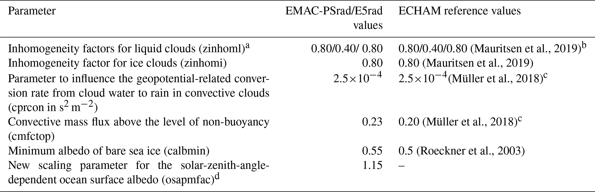
^a For radiation calls with the old radiation scheme, E5rad, zinhoml is calculated based on total liquid water path and another parameter (zinpar), according to Eqs. (11.52)–(11.53) in Roeckner et al. (2003). ^b Mauritsen et al. (2019) only discern certain shallow convective clouds with a different zinhoml factor; this is accounted for by setting two of the three zinhoml parameters to 0.8 in our simulations. ^c Here, we cite the parameters as listed for MPI-ESM1.2-LR by Müller et al. (2018). ^d Only applicable for simulations driven by PSrad.

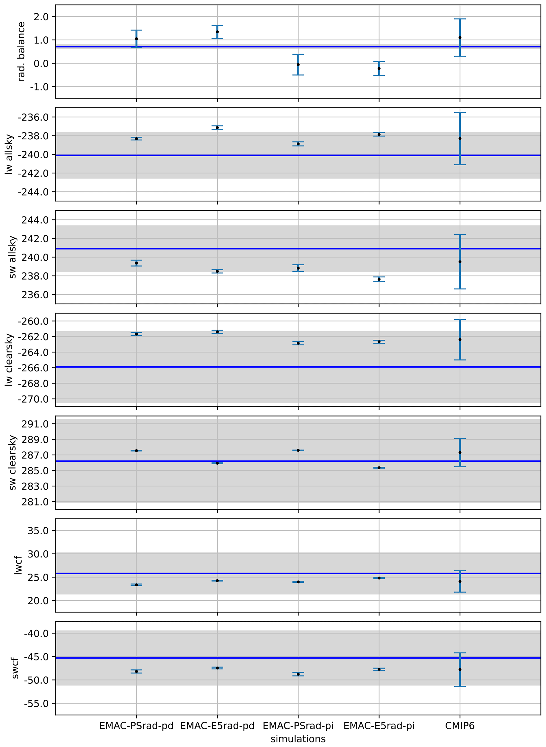
Figure 4 Radiation fluxes (in W m⁻²) for the pi and pd simulations driven by E5rad and PSrad in comparison to estimates from observational data. The estimates (horizontal blue lines) are based on Loeb et al. (2018), with updates presented by the CERES Science Team (2021). The grey shading marks the respective uncertainties, and we aimed for the radiation fluxes (mainly from the pd simulation) to be located within the shaded region after completion of the optimization process. CMIP6 data from Wild (2017) shows the multi-model mean and the inter-model standard deviation.

Figure 4 shows various radiation fluxes, along with reference values from observations (Loeb et al., 2018; CERES Science Team, 2021) and results from CMIP6 (Wild, 2017). Both the observations and the CMIP6 results in Wild (2017) are representative of present-day conditions. The global mean radiation (im)balance in the EMAC simulations is somewhat above 1 W m⁻² for present-day conditions and somewhat below 0 W m⁻² for pre-industrial conditions, with slightly more deviation from the target values for the E5rad simulations. The absolute values of the LW and SW all-sky fluxes are slightly too low on average in the EMAC simulations compared to observational data. Overall, the various fluxes from the optimized simulations lie close to or within the uncertainty range of observations.

3.3 Comparison of old and new model configuration

After optimizing the model configurations for pre-industrial and present-day conditions, we compare the climatological mean states of key meteorological quantities with reanalysis and observational data. For the reanalysis data, we employ ERA5 (Hersbach et al., 2020) monthly mean data on pressure levels (Hersbach et al., 2023) obtained from Copernicus Climate Change Service, Climate Data Store (2023). The model data were interpolated vertically to the pressure levels of the reanalysis (pressure level) data set, whereas the ERA5 data were horizontally regridded to the T42 resolution of the model data. For the evaluation of simulated precipitation data, we use the monthly mean observational data from the Global Precipitation Climatology Project (GPCP; e.g. Huffman et al., 1997, 2009; Adler et al., 2003) version 2.3 (Adler et al., 2018). For both reanalysis and observational data, we use the period 2000–2009 for intercomparison with the last 10 years of our simulations (see Sect. 3.1).

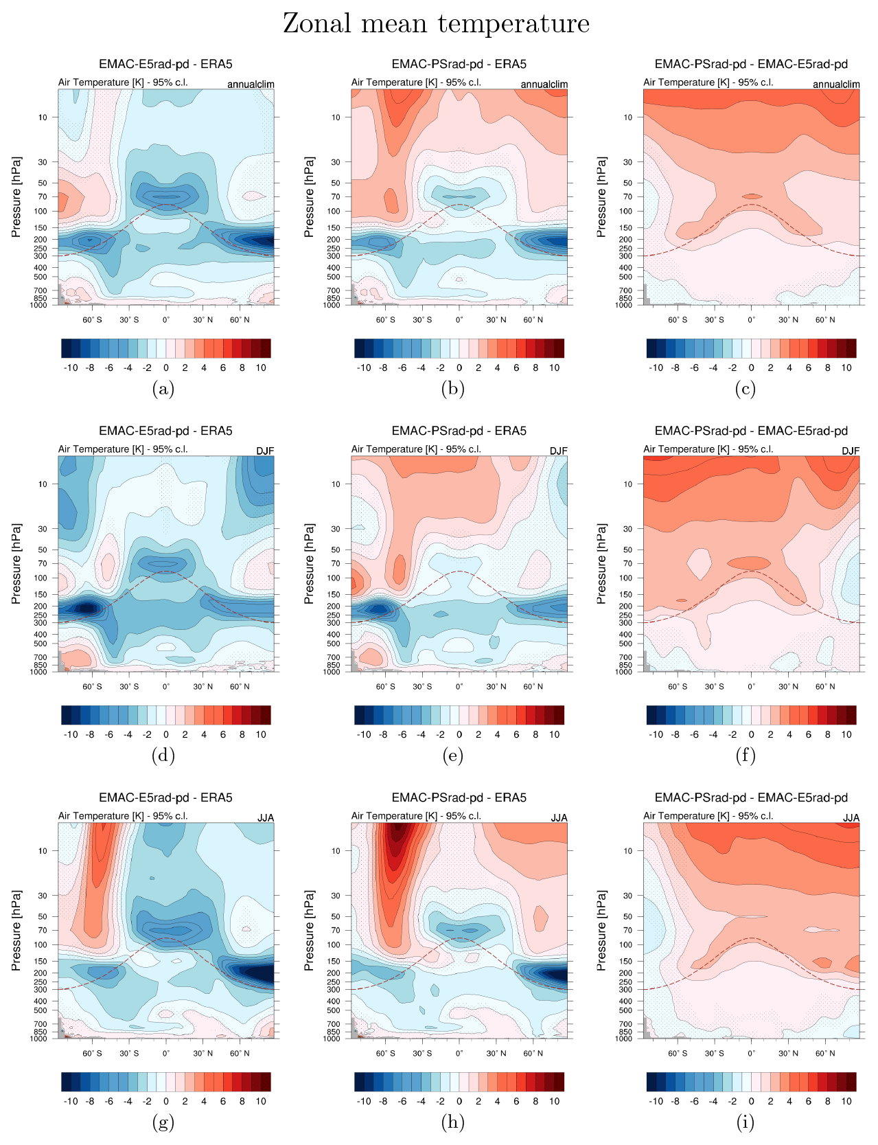
Figure 5 Differences in the multiannual zonal mean temperatures between EMAC-E5rad-pd and ERA5 (a, d, g), EMAC-PSrad-pd and ERA5 (b, e, h), and the differences between EMAC-E5rad-pd and EMAC-PSrad-pd (c, f, i). Differences in the annual means are shown in panels (a)–(c), whereas panels (d)–(f) and (g)–(i) show differences for December–January–February (DJF) and June–July–August (JJA) means, respectively. Stippled regions are not significant at the 95 % level based on Welch's t test. The dashed line indicates a simple latitudinally dependent approximation of the tropopause (Jöckel et al., 2000).

Figure 5 shows the differences in the zonal mean temperatures between the model present-day configurations and ERA5 (first two columns) and between the two present-day simulations with different driving radiation schemes (PSrad and E5rad; third column). Up to around 30 hPa, both model configurations show similar bias patterns compared to ERA5. These biases tend to be lower for EMAC-PSrad-pd than for EMAC-E5rad-pd, except for the extratropical stratosphere in the height region between 150 and 30 hPa. Above 30 hPa, EMAC-PSrad-pd shows mostly higher temperatures than EMAC-E5rad-pd. Hence, where E5rad was on average too cold in the region above 30 hPa, the EMAC-PSrad-pd simulation results seem to be too warm in comparison with ERA5 data, and the warm bias at 60–40° S during June–July–August (JJA) compared to ERA5 is even more pronounced in EMAC-PSrad-pd. However, in large regions, EMAC-PSrad-pd performs better, e.g. concerning the cold bias around the tropical cold point (which is reduced by about 3 K) and the reduced cold bias in the extratropical lower stratosphere.

The cold bias in the tropical upper troposphere and lower stratosphere, as well as other biases of EMAC-E5rad-pd compared to ERA5, is similar to what has been found by Jöckel et al. (2016) when comparing annual climatologies of EMAC simulations with ERA-Interim data (see their Fig. 12 and, in particular, the panel for the RC1-base-01 simulation). Previous comparisons of ECHAM5 and ERA-Interim data for December–January–February (DJF) presented by Stevens et al. (2013) show similar biases as our EMAC-E5rad-pd simulation (see their Fig. 12). Stevens et al. (2013) also find a resolution-dependent warming and a reduction in the cold biases during DJF when ECHAM6.1 (including an updated radiation scheme compared to ECHAM5) is employed. These changes from ECHAM5 to ECHAM6.1 are similar to the improvements we have found when assessing EMAC-PSrad-pd compared to EMAC-E5rad-pd simulations.

Figure 6 As in Fig. 5 but for the differences in the multiannual zonal mean of zonal winds.

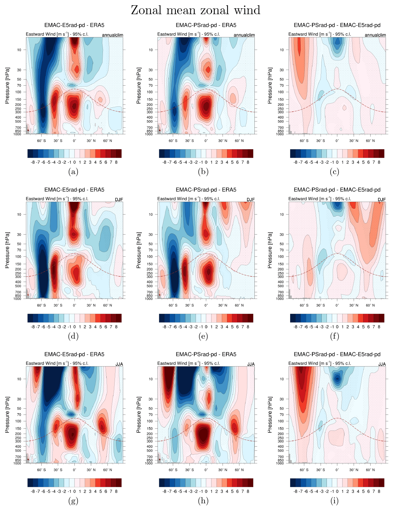
Figure 6 shows the corresponding zonal mean zonal wind differences. The main biases between the model data and ERA5 remain unchanged when the newly available radiation scheme, PSrad, is used. These biases have already been present in comparisons of ERA-Interim data with ECHAM5 and ECHAM6.1 data (Stevens et al., 2013; see their Fig. 13). EMAC-PSrad-pd shows reduced biases at 60° S in comparison to EMAC-E5rad-pd. However, in the Southern Hemisphere (SH) polar region during JJA above 50 hPa, the positive bias is increased in EMAC-PSrad-pd. In the tropical upper troposphere, eastward winds are present in EMAC-E5rad-pd, whereas ERA5 shows westward winds in this region. This bias slightly increases in the simulation with PSrad. Differences between EMAC-E5rad-pd and EMAC-PSrad-pd show increased wind speeds during JJA in the SH polar vortex (Fig. 6i). This strengthening of the polar vortex is desirable, as the polar vortex in EMAC is known to be too weak (Jöckel et al., 2016).

Although the analyses only include the last 10 years of both the E5rad-pd and the PSrad-pd simulation, the results from the pre-industrial simulations support the general features presented here. In particular, the patterns of the differences that arise when employing the new radiation scheme (PSrad) and the previous ECHAM5 scheme (E5rad) are similar under present-day and pre-industrial conditions.

Figure 7 shows specific humidity profiles (in kg kg⁻¹ of moist air) for different latitudinal bands from the tropics to the high latitudes. Overall, all data sets show the typical decrease in the specific humidity with height in the troposphere. Above approximately 100 hPa, ERA5 shows higher specific humidity than the model data. At this altitude, the EMAC-PSrad-pd simulation is moister (and thus in better agreement with ERA5) than the EMAC-E5rad-pd simulation, which is consistent with higher tropical cold-point temperatures in the EMAC-PSrad-pd simulation compared to the EMAC-E5rad-pd simulation (see Fig. 5). In general, ERA5 reaches the low stratospheric humidity values somewhat below (at higher pressures than) the model data. This is particularly obvious in the Northern Hemisphere (NH) and SH polar cap profiles, where, in the height region near 200 hPa, ERA5 has already reached minimum specific humidity values in the range of 2–3 × 10⁻⁶ kg kg⁻¹, and the EMAC simulations still show a roughly linear decrease in specific humidity (in log–log) up to somewhat below 100 hPa. Due to a slower decrease and a slight kink in the specific humidity profiles over the polar cap regions in the EMAC simulations, specific humidity values are higher in the EMAC simulations than in ERA5 around 200 hPa over the polar caps. After reaching the minimum specific humidity values in the upper troposphere–lower stratosphere region, the specific humidity values increase slightly with height. We attribute this increase to the moistening through methane oxidation, which increases with height up to at least 10 hPa in the model (Eichinger and Jöckel, 2014; see their Fig. 8).

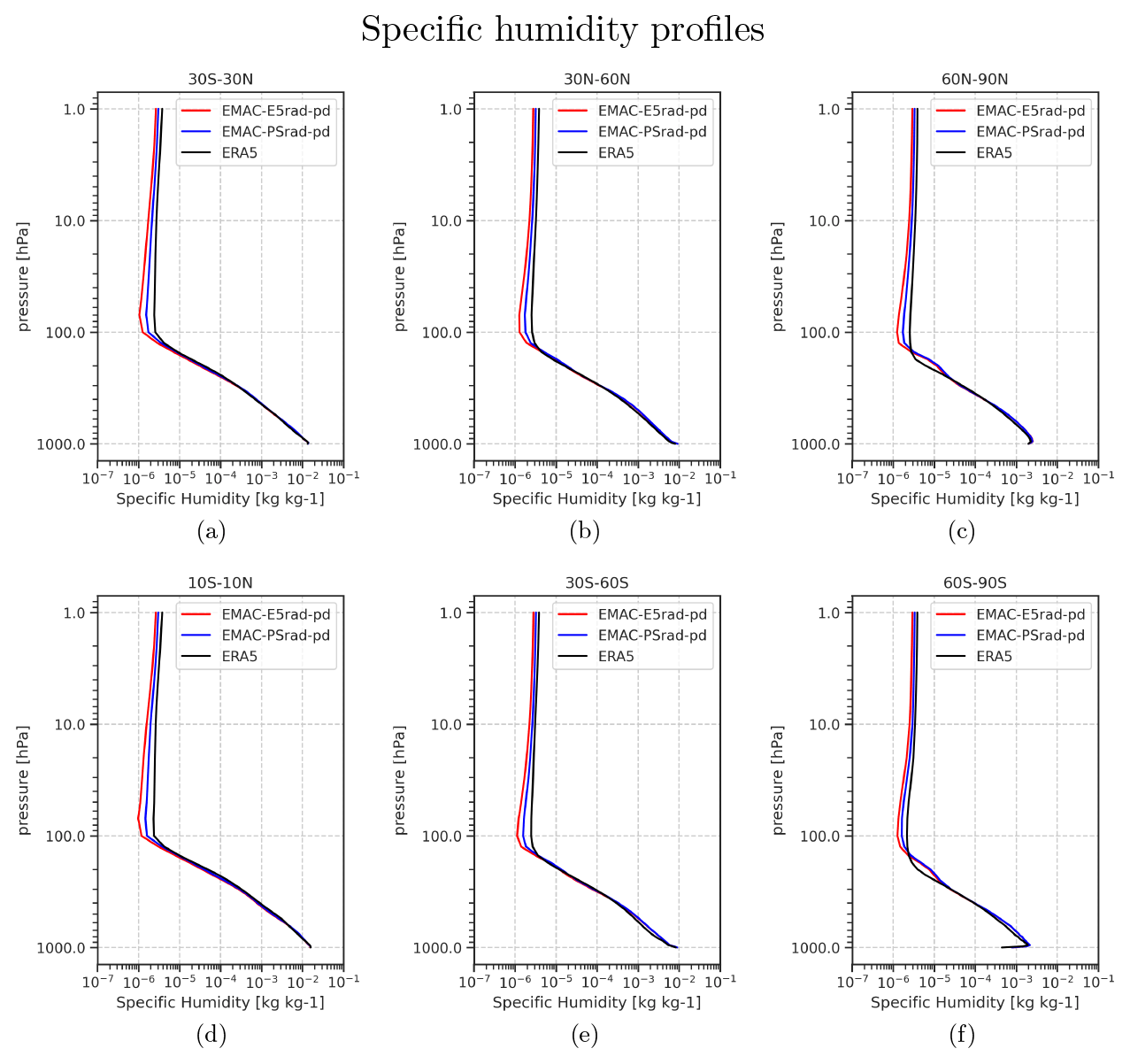
Figure 7 Profiles of specific humidity (kg kg⁻¹) for various latitudinal bands based on a 10-year climatology. The bands are for the tropics 30° N–30° S (a) and 10° N–10° S (d), the extratropics 30–60° N/S (b/e) and the polar region 60–90° N/S (c/f).

Seasonal variations in the tropical stratospheric water vapour related to the water vapour tape recorder (Mote et al., 1996) are shown in Fig. 8 for the last 10 years of the EMAC simulations and the period from 2000 to 2009 for ERA5. An intercomparison is feasible due to the selection of the transient SSTs and the nudging of the QBO in the EMAC simulations (see Table 1). The left panels (Fig. 8a and c) show the time series of specific humidity at 70 and 50 hPa averaged over 10° N–10° S. All data sets show a clear seasonal variation, and as noted before, EMAC-PSrad-pd shows higher values than EMAC-E5rad-pd, which are in better agreement with ERA5. The amplitudes of the seasonal cycle of stratospheric water vapour are largest in ERA5 and smallest in the EMAC-E5rad-pd simulation. According to Brinkop et al. (2016), this can be attributed to the tropical cold-point temperatures that are too low in EMAC-E5rad-pd. From comparing Fig. 8a and c, the time lag of the water vapour signal propagation is apparent. Furthermore, the amplitudes of the water vapour variations decrease with height in all data sets, as can be expected (Mote et al., 1996, 1998).

To assess the amplitude of the variations, Fig. 8 also shows the relative anomalies of specific humidity for the same region (Fig. 8b and d). We calculated the relative anomalies as $\left(q\right(t)-\stackrel{\mathrm{‾}}{q})/\stackrel{\mathrm{‾}}{q}$, where q(t) is the monthly specific humidity value, and the overbar denotes the mean (all months weighted equally) of the displayed period. The amplitude and signal strength are captured better in EMAC-PSrad-pd than in EMAC-E5rad-pd when taking ERA5 as a reference. Similar to the absolute amplitudes, the relative amplitudes also decrease with height.

Due to a setup inconsistency, ERA5 has a cold bias in the stratosphere for the period 2000 to 2006, which also affects stratospheric water vapour (Simmons et al., 2020). This issue has been addressed in a new set of analyses called ERA5.1 covering this period (Simmons et al., 2020). We note, however, that the differences between ERA5.1 and ERA5 regarding temperatures and water vapour as analysed by Simmons et al. (2020) are relatively small compared to the differences we see between ERA5 and our model simulations. Hence, we simply applied the ERA5 data, as the main conclusions regarding the model reanalyses differences will remain unchanged.

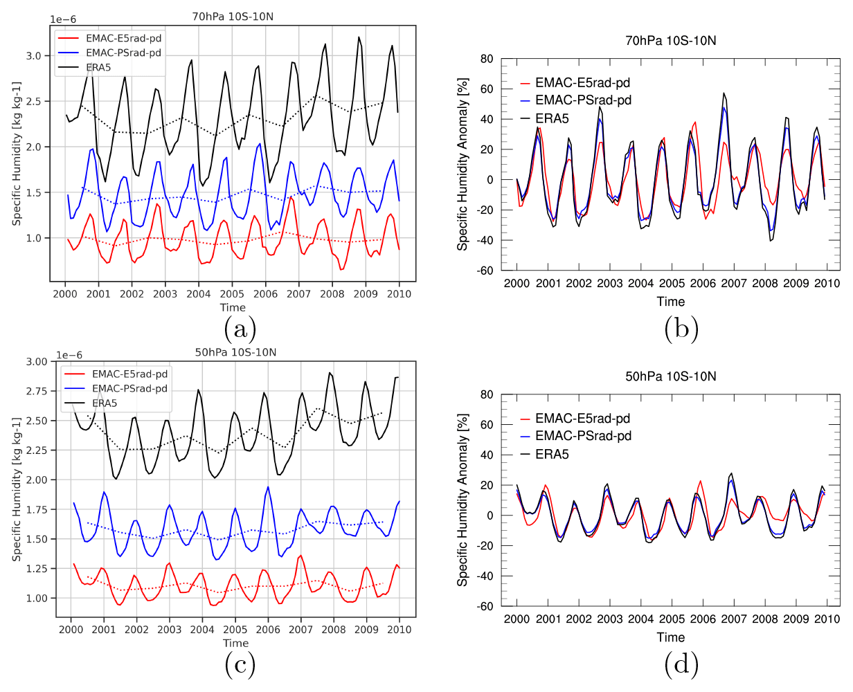
Figure 8 Tape recorder signal at 70 hPa (a, b) and 50 hPa (c, d) given by the specific humidity averaged over 10° N–10° S. (a, c) Time series of specific humidity in 10⁻⁶ kg kg⁻¹. (b, d) Relative anomaly (in percent) of the tape recorder signal; i.e. displayed is the relative anomaly with respect to the respective long-term mean (all months weighted equally).

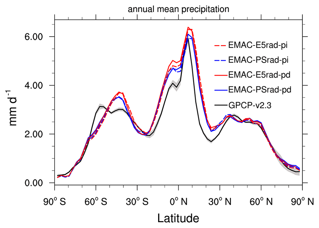
Figure 9 Multiannual zonal mean precipitation (mm d⁻¹) for the last 10 years of the simulations and the period 2000–2009 for GPCP v2.3 data. GPCP v2.3 was conservatively regridded to a T42 grid using Climate Data Operators (CDO; https://code.mpimet.mpg.de/projects/cdo/, last access: 21 August 2023).

Table 4 Annual mean precipitation (mm d⁻¹) over the last 10 years of the simulations and for 2000–2009 for GPCP 2.3 data.

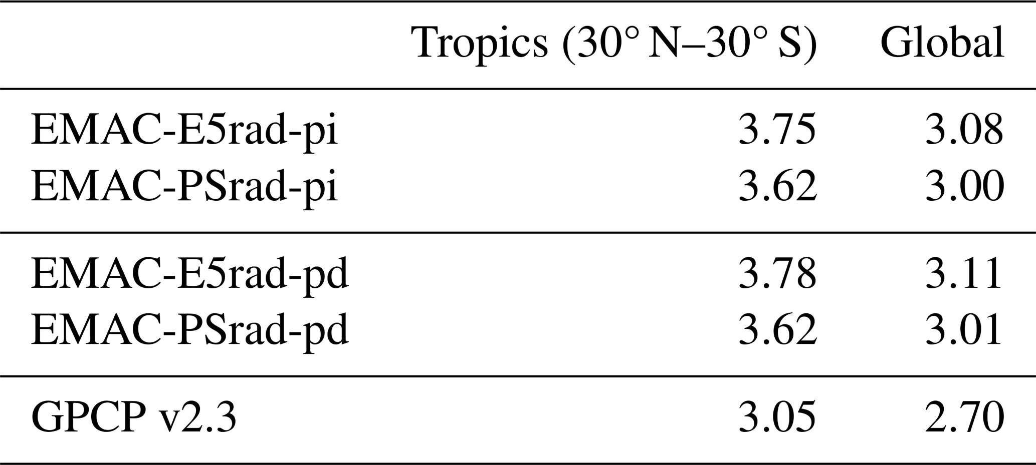
Figure 9 shows the 10-year mean zonal mean precipitation for the model data and GPCP v2.3. Table 4 presents the corresponding tropical (30° N–30° S) and global means. Overall, the largest differences between model and observational data are found in the tropics (30° N–30° S) and in the region 40° S–70° S. In the tropics, all simulations show enhanced precipitation in comparison to the observational data. On average, the tropical (30° N–30° S) mean precipitation lies between 3.62 and 3.78 mm d⁻¹ in the simulations, whereas GPCP v2.3 shows 3.05 mm d⁻¹. Furthermore, the different simulation periods of pi and pd seem to have a smaller impact on the precipitation distribution than the exchange of the radiation scheme; i.e. blueish (reddish) lines are more similar than solid (dashed) lines, respectively. The global mean precipitation is 3.00–3.11 mm d⁻¹ in the simulations and 2.70 mm d⁻¹ in the GPCP v2.3 data. Both the distribution of simulated precipitation and the global and tropical mean values are comparable to previous EMAC results presented by Jöckel et al. (2016) (their Fig. 13), where only EMAC simulations which include global mean temperature nudging showed considerably less precipitation.

4 Radiative forcing calculations using multiple diagnostic calls

We use the simulations of the newly optimized model configurations to assess RFs due to perturbations of GHGs in the old and new model setups.² A central objective of the intercomparison presented here is to enable the attribution of differing RF results either to differences in the background meteorology or to differences in the actual radiative transfer calculation, as well as to assess the impact of different GHG backgrounds on the RF values related to a perturbation. To this end, additional diagnostic calls of the radiation scheme with perturbed GHGs (namely CO₂, N₂O, CH₄, and CFCs) have been conducted in the simulations under pre-industrial and present-day conditions. This was done for the simulations which employ E5rad as the driving radiation scheme (EMAC-E5rad-pi and EMAC-E5rad-pd), as well as for the simulations which employ PSrad (EMAC-PSrad-pi and EMAC-PSrad-pd). The respective GHG fields were adopted from previous EMAC simulations (see Table 1), except for the methane field which enters the first call of the radiative transfer calculation and drives the simulation (see Sect. 3.1).

Table 5 lists the respective perturbations that are calculated in the multiple calls of the radiation scheme. In total, 22 additional (diagnostic) calls for calculating instantaneous RF (calls 02 to 23) and 11 additional calls for calculating stratospheric-adjusted RF (calls 24 through 34, where stratospheric adjustment is calculated as described by Stuber et al., 2001) were conducted. In the columns of Table 5, the perturbations are listed; for example, for call 03 (call 25), CO₂ has been set to present-day values for the pi simulations and to pre-industrial values for the pd simulations. Thus, the instantaneous (stratospheric-adjusted) RF due to increasing CO₂ from pre-industrial to present-day levels can be assessed from $F_{\mathrm{pi};{\mathrm{CO}}_{\mathrm{2}}\left(\mathrm{pd}\right)}-F_{\mathrm{pi}}$ or alternatively from $F_{\mathrm{pd}}-F_{\mathrm{pd};{\mathrm{CO}}_{\mathrm{2}}\left(\mathrm{pi}\right)}$. The first subscript denotes the reference state, the second subscript (if present) denotes the species that has been perturbed, and F denotes the instantaneous (stratospheric-adjusted) TOA radiative fluxes from call 02 and call 03 (call 24 and call 25), respectively. This may be viewed as the adoption of the forward and backward calculation method (known from radiative feedback analysis; for example, Colman and McAvaney, 1997; Klocke et al., 2013; Rieger et al., 2017) for the RF calculation, which allows us to assess the effect of the GHG background on the diagnosed forcing.

Additionally, for the calculation of instantaneous RFs, diagnostic calls with a “switched” radiation scheme have been performed. This means that the radiation scheme driving the simulation and the radiation scheme used in a diagnostic call are different. For example, calls 13 and 14 from the EMAC-E5rad-pi simulation can be used to evaluate the instantaneous RF of present-day CO₂ using the PSrad radiation scheme in a pre-industrial simulation which is driven by E5rad. This provides the opportunity to further assess the dependence of the RF results on the background (here this does not refer to present-day vs. pre-industrial but rather the different meteorological climatologies from the models that serve as different backgrounds) or the employed radiation scheme.

Table 5 Employed radiation perturbations for the four EMAC simulations. The first call drives the respective simulation, and calls 02–12 are used for calculating various instantaneous RFs due to the perturbation of GHGs. Calls 13–23 allow us to assess the RFs of the same perturbation with the switched radiation scheme, whereas calls 24–34 allow us to assess the stratospheric-adjusted RFs.

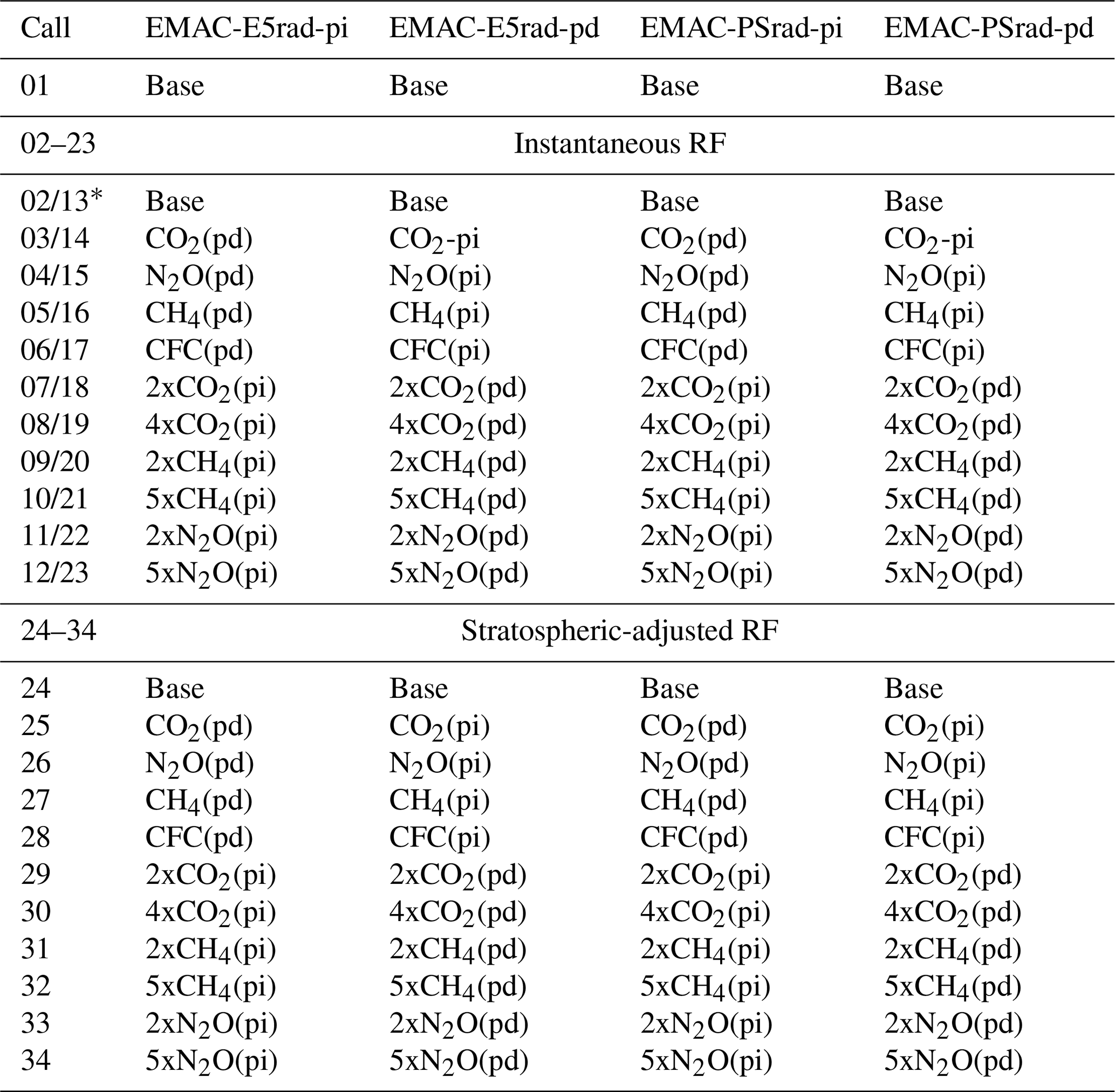
^* The first number refers to the call with the driving radiation scheme, and the second number refers to the call with the switched radiation scheme.

Table 6 shows the instantaneous and stratospheric-adjusted RF means for the last 10 years of the simulation for different GHG perturbations. In the calls in which a single GHG is doubled, quadrupled, or quintupled, the increase relates to the respective base period of the simulations; i.e. for the 2xCH₄ experiments, the CH₄(pi) values have been doubled for the pi simulations, whereas the CH₄(pd) values have been doubled for the pd simulations. Note that in this table the forcings are calculated with the same radiation scheme that is also driving the GCM-type simulation. For instantaneous RFs, we will also address (somewhat later in the paper) the results from RF calculations which result from switching the radiation scheme (Table 8).

We start our evaluation by comparing stratospheric-adjusted RFs from our simulations (columns 2 to 5 in Table 6) with idealized estimates (two rightmost columns in Table 6) which are based on formulas presented by Etminan et al. (2016). Overall, the results from the simulations using PSrad are closer to the Etminan-based estimates concerning stratospheric-adjusted RF. In particular, this is true for the assessment of stratospheric-adjusted RFs from CH₄(pi) and 2xCH₄, which are substantially higher in PSrad than in E5rad, and for 4xCO₂, which are lower in PSrad than in E5rad. We note here that the estimates given in parentheses are outside the recommended range of the formulas, as indicated by Etminan et al. (2016). We nevertheless present these values as they provide additional evidence that the PSrad scheme yields much more realistic stratospheric-adjusted RF values, especially for CH₄ and (see below) N₂O perturbations. The instantaneous and stratospheric-adjusted RF values due to doubling or quadrupling CO₂ from the EMAC-E5rad-pd simulation are in agreement with previous results obtained with EMAC and the ECHAM5 radiation scheme, as presented by Dietmüller et al. (2014) and Rieger et al. (2017; see the forward results in both studies).

Additional stratospheric-adjusted and instantaneous RFs for 2xCO₂ and 3xCH₄ from global model simulations have been presented by Richardson et al. (2019). Please see their Sect. 2 on how the respective forcings were defined, and note that they (mostly but not exclusively) use the present day as the reference state. For the latter reason, we will address results from our pd simulations for comparisons only. For the 2xCO₂ RFs, the results from our EMAC-PSrad-pd simulation are closer to the values presented by Richardson et al. (2019) than the RFs based on EMAC-E5rad-pd for both instantaneous and stratospheric-adjusted RFs. For 3xCH₄ RFs, the results from our EMAC-E5rad-pd simulation (0.24 and 0.3 W m⁻² for instantaneous RF and stratospheric-adjusted RF, respectively; interpolated from the 2xCH₄ and 5xCH₄ RFs) show clearly lower values than the results from the EMAC-PSrad-pd simulation (0.97 and 0.95 W m⁻², respectively; interpolated as before). The increased RFs associated with a 3xCH₄ experiment, as diagnosed from PSrad, are in better agreement with the values presented by Richardson et al. (2019), which are somewhat above 1 W m⁻².

Another aspect to note about the methane RFs is that with E5rad the stratospheric temperature adjustment acts to increase the RF in comparison to the instantaneous RF, whereas for PSrad the differences between instantaneous and stratospheric-adjusted RF are smaller, and the sign depends on the background state. PSrad includes SW absorption of methane in two bands in the near-infrared (3.08–3.85 and 2.15–2.50 µm; see the RRTM bands described in the ECHAM6 documentation; Giorgetta et al., 2013). The SW absorption acts to counteract the stratospheric cooling induced by the LW radiation (Byrom and Shine, 2022, see their Fig. 2). Hence, the adjustment difference we find between PSrad and E5rad is in part consistent with the results from (Smith et al., 2018, see their Fig. S6). They point out that for the same experiments as the ones analysed by Richardson et al. (2019), the rapid radiative adjustment induced by the stratospheric temperature adjustment is negative in models with the explicit treatment of methane SW absorption in the radiation scheme and positive in models without. However, in the latter case, the increase reported by Smith et al. (2018) is more pronounced as there is a substantial additional contribution from cloud radiative adjustments that are not covered by our technique.

The instantaneous RF of 3xN₂O with respect to present-day conditions has been assessed by Hodnebrog et al. (2020) for global models and LBL calculations. They find an instantaneous RF of roughly 1.5 and 1.4 W m⁻², respectively. Interpolation of the instantaneous 2xN₂O and 5xN₂O calculations from EMAC-E5rad-pd and EMAC-PSrad-pd yields values of 2.49 and 1.37 W m⁻², respectively, clearly emphasizing the superiority of N₂O forcings provided by the latter.

Table 6 RFs (W m⁻²) for perturbations based on the diagnostic radiation calls described in Table 5 for the last 10 years of the simulations. In addition, best estimates based on the formula from Etminan et al. (2016) are given as reference values for stratospheric-adjusted RF.

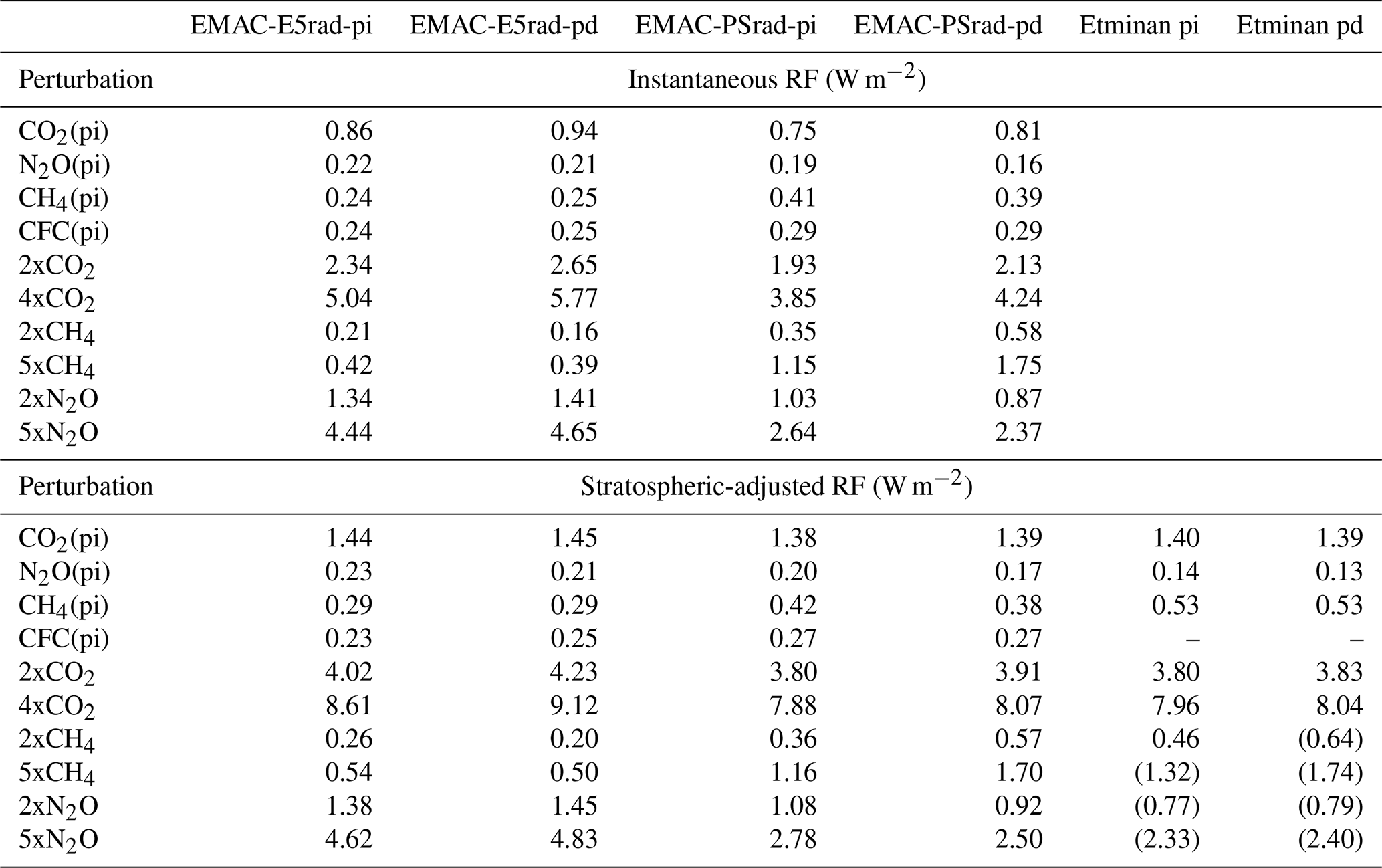
The interannual standard deviations were of the order of 0.01 W m⁻². Values in parentheses in the columns Etminan pi and Etminan pd are for perturbations that are outside the valid range of the approximation formulas given by Etminan et al. (2016). The perturbations 2xN₂O(pi) and 2xCH₄(pd) are close to the valid range.

Table 7 shows the global mean clear-sky instantaneous RFs corresponding to the all-sky instantaneous RFs presented in Table 6. Our results can be compared with those from Pincus et al. (2020), which were derived from the multi-model mean of so-called “benchmark” models. Based on the description by Pincus et al. (2020), we can compare the results from EMAC-E5rad-pd and EMAC-PSrad-pd shown in Table 7 with their results for clear-sky instantaneous RF due to increasing a single GHG from pre-industrial to present-day values. However, as the base periods and values for pi and pd conditions are different (for example, Pincus et al., 2020, use 2014 as pd), we rescaled our clear-sky RF results to allow for a better comparison. The corresponding values are listed in parentheses in Table 7. For the rescaling, we assumed that the 2014 values used by Pincus et al. (2020) are similar to the values presented by Meinshausen et al. (2017). Consequently, the clear-sky instantaneous RFs were adjusted as follows: ${\mathrm{iRF}}_{\mathrm{cs}}^{*}={\mathrm{iRF}}_{\mathrm{cs}}\cdot \mathrm{\Delta }{X}_{\mathrm{P}\mathrm{20}}/\mathrm{\Delta }{X}_{\mathrm{N}\mathrm{23}}$, where iRF_cs refers to the instantaneous clear-sky RF, and the asterisk denotes the corresponding rescaled quantity. ΔX denotes the change (in mol mol⁻¹) of the species X from pi to pd conditions, and the subscripts P20 and N23 refer to Pincus et al. (2020) and our study, respectively. Taking into account the rescaling, all clear-sky RFs for the pi experiments calculated with PSrad are closer to the results presented by Pincus et al. (2020) than the results obtained with E5rad. As an example, the global mean clear-sky RF (including the above-mentioned correction), due to the rise in methane from pi to pd, increases from 0.41 W m⁻² in the E5rad simulation to 0.51 W m⁻² in the simulation with PSrad and is closer to the reference value of 0.67 W m⁻² presented by Pincus et al. (2020). Conversely, for N₂O the clear-sky instantaneous RF decreases when PSrad is used and is thus in better agreement with the value of approximately 0.21 W m⁻² presented by Pincus et al. (2020).

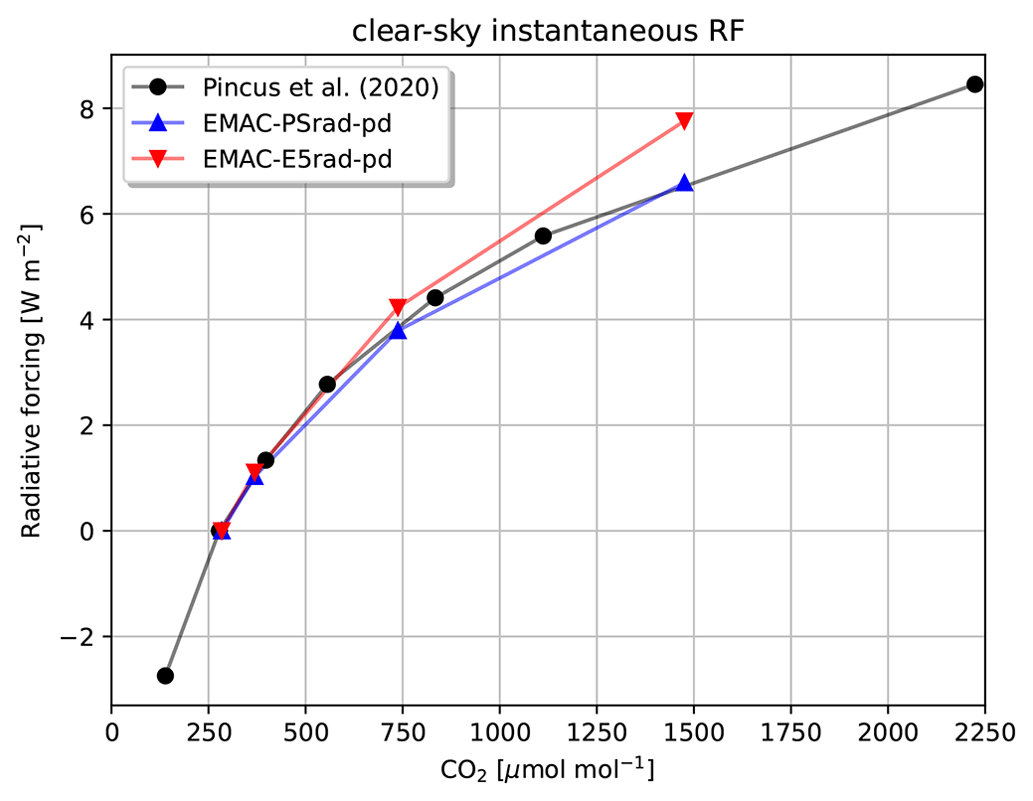
Figure 10 Clear-sky instantaneous RF for CO₂-folding experiments from our pd simulations compared to benchmark values from Pincus et al. (2020). The reference background is given by pd conditions, which differ slightly between our study and the study by Pincus et al. (2020). Furthermore, for the pd conditions of Pincus et al. (2020) in 2014, we assumed the respective values according to Meinshausen et al. (2017); see text for details. Note that clear-sky instantaneous RF is calculated with respect to a pd background for all non-CO₂ greenhouse gases and pi conditions for CO₂.

Pincus et al. (2020) also show clear-sky RFs with respect to CO₂-folding experiments. Presuming that they use pre-industrial CO₂ as a reference state for CO₂, whereas the other GHGs and the meteorology are representative of present-day conditions, one can try to compare their results with our rescaled results for the CO₂-folding experiments performed in the EMAC-E5rad-pi and EMAC-PSrad-pi simulations. This would lead to a seemingly better agreement of E5rad than PSrad results with their values. However, we warrant that this comparison is questionable due to the following: (i) We have a different GHG (including water vapour) background, namely pi, in comparison to their background of pd conditions. We assume that through saturation we would get lower RFs (i.e. a reduced sensitivity to CO₂ changes) than presented here if the CO₂-folding were performed against a pd GHG background. (ii) In the climatological pd background, the tropospheric temperatures are likely higher and the stratospheric temperatures lower than for our pi background. Here, we reason that both changes will likely lead to an increased RF as diagnosed from CO₂-folding experiments, with the stratospheric component potentially making the larger contribution (He et al., 2023).

An estimate of the combined effect can be obtained when comparing our “forward” and “backward” experiments for calculating the clear-sky RF due to the increase in a single GHG from pi to pd levels. For both E5rad and PSrad, the clear-sky RF due to the rise in the CO₂ from pi to pd levels is higher when assessed against the pd background. For N₂O, the relation is reversed, whereas for CFCs there is (almost) no dependence of the instantaneous clear-sky RF on the background. Interestingly, for CH₄ the clear-sky instantaneous RFs are higher for a pd background when assessed with E5rad, and lower when assessed with PSrad compared to the RFs when calculated against a pi background. Qualitatively similar dependencies of the instantaneous RFs on the GHG background are found for the all-sky fluxes (see Table 6).

Alternatively, for the comparison of clear-sky CO₂ RFs with the benchmark results presented by Pincus et al. (2020), we can also employ the CO₂-folding experiments from our pd background simulations. This has the advantage that the background with respect to which the RF of the CO₂-folding experiments is calculated is comparable between the studies. However, it comes with the drawback that the sampling points with respect to which CO₂-folding RFs are determined differ. Figure 10 shows the corresponding results which indicate that the EMAC-E5rad-pd simulation does not show better clear-sky instantaneous RFs compared to EMAC-PSrad-pd simulation. In particular, for extreme CO₂-folding experiments, the simulation with PSrad seems to produce better results than the simulation with E5rad.

Table 7 Global mean clear-sky instantaneous RFs (W m⁻²) for perturbations based on the diagnostic radiation calls described in Table 5 for the last 10 years of the simulations. Values in parentheses denote rescaled EMAC clear-sky RFs which are supposed to ensure better comparability with the RFs presented by Pincus et al. (2020). See text for details.

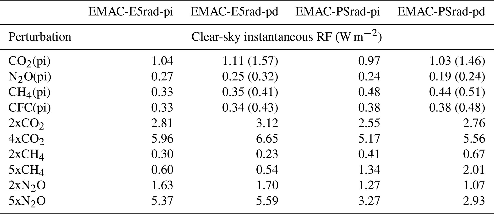
The interannual standard deviations were of the order of 0.01 W m⁻².

The instantaneous RFs presented in Table 6 are complemented by Table 8, which arises when the instantaneous RF is calculated with a different radiation scheme compared to the scheme that is driving the simulation. Hence, the columns of Tables 6 and 8 can be compared to each other on a one-to-one basis. Overall, the relative differences are roughly 10 % or less, showing that the results are relatively robust to changes in the background state related to switching the radiation scheme. With respect to experiments that assess the instantaneous RF due to an increase in a single GHG from pi to pd levels, we find that the changes in the meteorological background associated with the radiation scheme do not play a major role. For CFCs, N₂O, and CH₄, they are almost negligible, whereas they are somewhat larger for CO₂ (the respective values in Tables 6 and 8 are almost identical, except for the CO₂ perturbations).

Related to the dependence of RFs for CO₂ perturbations on the background, we have previously detected a larger CO₂ sensitivity in the E5rad compared to the PSrad simulations. As discussed above, for the dependence of the instantaneous CO₂ RFs on the pi and pd background, we point out that a warmer stratosphere in the PSrad compared to the E5rad simulations might be contributing to the lower RF values diagnosed from PSrad compared to E5rad. In line with this argument, instantaneous all-sky CO₂ RFs increase (decrease) for E5rad (PSrad) when the background is provided by the switched radiation scheme PSrad (E5rad), as can be seen from the comparison of Tables 6 and 8.

Table 8 Instantaneous RFs for perturbations described in Table 5 for the last 10 years of the simulations, where the radiation scheme for diagnosing the instantaneous RF was switched compared to the radiation scheme driving the simulation. As an example, in the second column, radiation calls with the E5rad scheme were used to calculate the instantaneous RFs within the EMAC-PSrad-pi simulation.

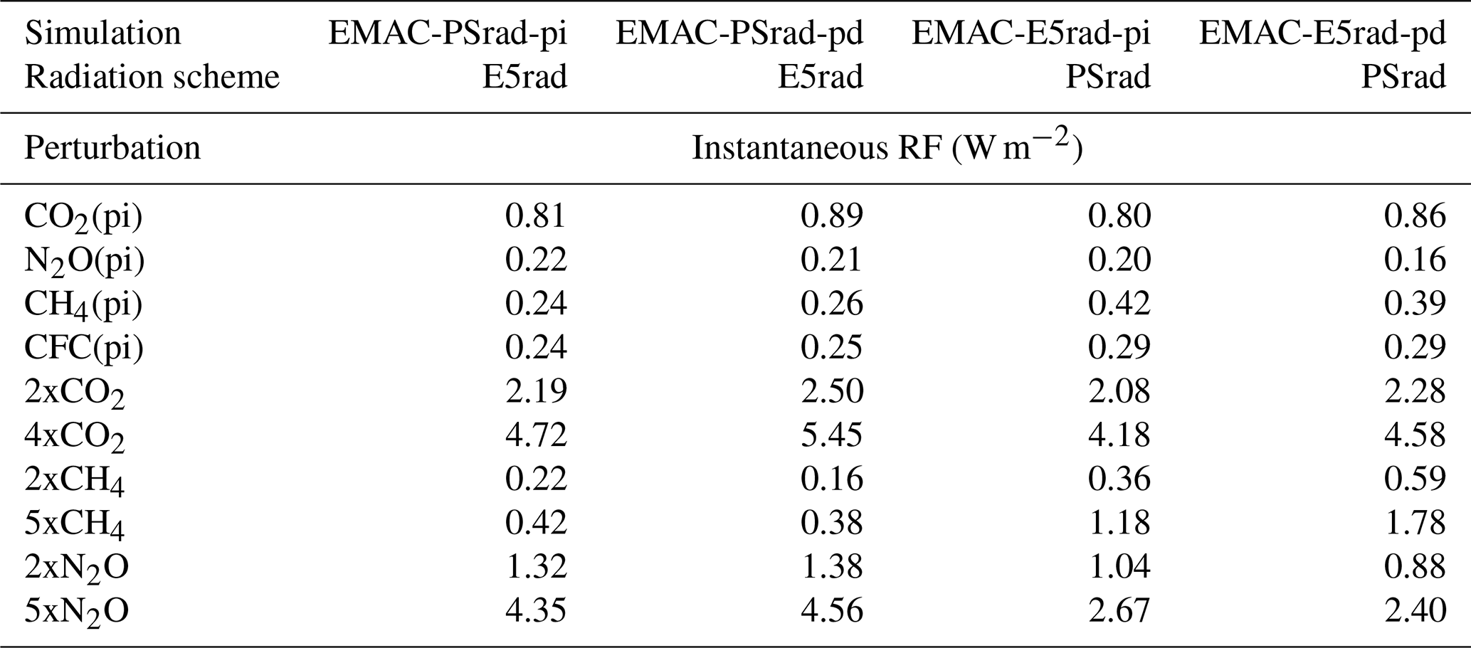
The interannual standard deviations were of the order of 0.01 W m⁻²

5 Summary and conclusions

In this paper, we describe the recent upgrades of the MESSy radiation infrastructure and its first applications. In Sect. 2, we give a detailed overview of the implemented changes. A guiding principle through the implementation process has been to retain the possibility of using all previous model setups (backward compatibility) and to also ensure the applicability of MESSy-specific features (e.g. multiple radiation calls) with the updated radiation infrastructure. Specific highlights of the new implementations are the integration of the radiation scheme PSrad and the availability of a new submodel ALBEDO, which features solar-zenith-angle-dependent albedos. Furthermore, a white sky albedo for snow-free land has been compiled based on satellite data.

Section 3.2 exemplarily describes the model optimization of a typical “old” (with ECHAM5 radiation) and “new” (with PSrad radiation) GCM-type setup (fixed sea surface temperatures and no chemistry, except for simplified methane chemistry) with a consistent set of parameters for pre-industrial and present-day conditions. Comparing the old and new setup, also with observational and reanalysis data, shows that the main features of the simulated climate (also known from previous ECHAM5 and other ECHAM6.1 simulations; e.g. Stevens et al., 2013) remain. However, some biases from the old model setup, e.g. the cold bias in the tropical upper troposphere–lower stratosphere and a polar vortex that is too weak in the Southern Hemisphere winter, are reduced when the PSrad scheme is employed.

Finally, we show radiative forcing results based on the old and the new model setups using multiple diagnostic radiation calls. In total, we perform 33 additional diagnostic radiation calls per simulation to assess various radiative forcings. In particular, we show stratospheric (temperature)-adjusted and instantaneous RF values due to reduced or increased greenhouse gases. When comparing these results with previous estimates, we find that PSrad generally performs better for instantaneous and stratospheric-adjusted radiative forcings. In particular, methane (nitrous oxide) radiative forcings calculated with PSrad are strongly increased (decreased) in comparison to the radiative forcings calculated with the ECHAM5 radiation scheme, which means a clear improvement when compared to benchmark results. For the instantaneous forcings, we also derive results for which the radiation scheme of the diagnostic calls is switched compared to the driving radiation scheme; i.e. using the old radiation scheme to propagate the simulation and evaluating two additional diagnostic radiation calls with the new radiation scheme to determine the instantaneous flux changes, or vice versa. It appears that changes in the radiative forcing results from the previous (ECHAM5) setup to the new (PSrad) setup are mainly attributable to the radiative transfer calculations themselves, whereas the changed background climatology related to the driving radiation scheme plays only a minor role.

The implemented changes lead to an improved representation of tropical upper tropospheric temperatures (and thus stratospheric water vapour). Furthermore, various radiative forcings due to greenhouse gas perturbations tend to be improved. In particular, this is the case for methane forcing experiments which show a higher radiative forcing with the new radiation scheme, PSrad, and are thus in better agreement with literature-based reference values. The latter can be exploited to better quantify methane radiative forcings and the role of methane as a feedback component in the climate system. The developments mark an important step for the MESSy framework to be able to include additional radiation schemes. The next steps concerning the use of the MESSy radiation infrastructure are to employ the PSrad scheme with interactive chemistry and an online coupled ocean (Earth system model setup). Further envisaged developments are the coupling of PSrad to FUBrad and the use of PSrad with an interactive aerosol model, which will be enabled by the revision of the AEROPT submodel.