ZJU-AERO V0.5: an Accurate and Efficient Radar Operator designed for CMA-GFS/MESO with the capability to simulate non-spherical hydrometeors

In this study, we present a new forward polarimetric radar operator called the Accurate and Efficient Radar Operator designed by ZheJiang University (ZJU-AERO). This operator was designed to interface with the numerical weather prediction (NWP) model of the global forecast system/regional mesoscale model of the China Meteorological Administration (CMA-GFS/MESO). The main objective of developing this observation operator was to assimilate observations from the precipitation measurement radar (PMR). It is also capable of simulating the ground-based radar's polarimetric radar variables, excluding the Doppler variables such as radial velocity and spectrum width. To calculate the hydrometeor optical properties of ZJU-AERO, we utilize the invariant-imbedding T-matrix (IITM) method, which can handle non-spherical and inhomogeneous hydrometeor particles in the atmosphere. The optical database of ZJU-AERO was designed with a multi-layered architecture to ensure the flexibility in hydrometeor morphology and orientation specifications while maintaining operational efficiency. Specifically, three levels of databases are created that store the single-scattering properties for different shapes at discrete sizes for various fixed orientations, integrated single-scattering properties over shapes and orientations, and bulk-scattering properties incorporating the size average, respectively. In this work, we elaborate on the design concepts, physical basis, and hydrometeor specifications of ZJU-AERO. Additionally, we present a case study demonstrating the application of ZJU-AERO in simulating the radar observations of Typhoon Haishen.

1 Introduction

The development of regional models with finer horizontal resolutions, such as the Chinese operational regional numerical weather prediction (NWP) model, known as the regional mesoscale model of the China Meteorological Administration (CMA-MESO) (Chen et al., 2008; Shen et al., 2023), necessitates the acquisition of more convective-scale information about the atmosphere to improve quantitative precipitation forecasts. Fortunately, the measurements from spaceborne and ground-based weather radars provide valuable sources of three-dimensional, kilometer-scale volume data with high temporal resolutions. However, weather radar can only observe the amplitude and phase of electromagnetic waves echoed from meteorological objects, specifically various types of hydrometeors. Except for the Doppler radar variables, such as radial velocity (beyond the scope of this study), it is challenging to establish a connection between the prognostic variables simulated by the NWP model and the observable polarimetric radar variables, which are inferred from the statistical moments of voltage time series collected by the receiver of the weather radar electronics system (Zhang, 2016).

The software package introduced in this work is referred to as a “forward radar operator”, designed to transform the model prognostic variables into the observation space, resulting in equivalent simulated synthetic radar variables. Utilizing a unified forward radar operator for assimilations and retrievals is believed to be superior to employing an ensemble of retrieval relationships along with pre-processing procedures and corrections for different frequencies and platforms. In essence, using radar data in the observation space is preferred over the model space due to the highly non-linear and non-unique nature of the processes that observational operator of polarimetric radar describes.

Several radar operators have been developed and published over the past several decades. For instance, Jung et al. (2008) implemented a polarimetric radar simulator known as the Polarimetric Radar data Simulator developed by the Center for Analysis and Prediction of Storms (CAPS-PRS) at the University of Oklahoma. This simulator uses spheroids to characterize hydrometeors and computes optical properties using online Rayleigh approximations or offline lookup tables (LUTs) constructed by the extended boundary condition method (EBCM) described in Mishchenko and Travis (1994). This simulator has been applied to low-frequency bands, such as the S, C, and X bands. Ryzhkov et al. (2011) described another radar operator for research purposes, specifically tailored for spectra-resolving cloud microphysics models, although it is more computationally expensive. Zeng et al. (2016) described an efficient radar operator that is online-coupled to the Consortium for Small-scale Modeling (COSMO) and Icosahedral Nonhydrostatic (ICON) weather and climate model, makes use of Mie/T-matrix scattering lookup tables of solid, liquid, and melting (mixed-phased) hydrometeors, and is named the Efficient Modular VOlume scanning RADar Operator (EMVORADO). While early versions of EMVORADO focus on non-polarimetric radar variables, later developments on EMVORADO have enabled its capability to simulate dual-polarization variables and conduct sufficient evaluations (Trömel et al., 2021; Shrestha et al., 2022). In addition to the above operators, Wolfensberger and Berne (2018) reported a cross-platform polarimetric radar operator termed a POLarimetric forward radar operator for the COSMO model (COSMO-POL). This operator was designed for the COSMO-NWP model and can simulate melting particles. The optical database of the COSMO-POL was constructed also using the EBCM, characterizing all hydrometeor particles as homogeneous spheroids. However, in the COSMO-POL, the hydrometeor orientations and shape parameter settings are fixed at the level of the optical database, which limits sensitivity testing and fine-tuning. Wang and Liu (2019) reported a forward reflectivity observation operator (together with its tangent linear and adjoint operator) with the simulation capability of frozen hydrometeors designed to assimilate the data of ground-based radar in the Weather Research and Forecasting Model (WRF) in which the simulated reflectivity is parameterized as fast-polynomial relationships with respect to the mixing ratios of hydrometeors. More recently, Oue et al. (2020) developed the Cloud-resolving model Radar SIMulator (CR-SIM), which can simulate polarimetric radar and light detection and ranging (lidar) observations for various cloud-resolving models (CRMs), including the WRF, ICON, the Regional Atmospheric Modeling System (RAMS), and the advective statistical forecast model (SAM). CR-SIM has a unique capability for explicitly representing the rimming procedure by coupling it with the prognostic variable known as the rimming ratio in the Predicted Particle Properties (P3) microphysics package (Morrison and Milbrandt, 2015). However, CR-SIM is currently limited to ground-based platforms and offers no explicit treatment for melting particles. Moreover, the fast-parameterized forward radar operator developed by Zhang et al. (2021) contains a melting scheme module for targeting data assimilation purposes.

This work aims to design a cross-band and cross-platform radar operator for research purposes, such as microphysics package validation, and operational data assimilation use in the global forecast system/regional mesoscale model of the China Meteorological Administration (CMA-GFS/MESO). The software prototype of this radar operator, hereafter referred to as the Accurate and Efficient Radar Operator designed by ZheJiang University (ZJU-AERO), essentially addresses the scattering computation of hydrometeors and the construction of an optical properties database as the key aspects in the evolution of the radar operator. We utilize a semi-analytical scattering computation approach of a T-matrix to ensure accuracy and feature a multi-layered optical database that includes single-scattering properties at discrete sizes and orientations, integrated single-scattering properties over shapes and orientations, and bulk-scattering properties incorporating the size average. Additionally, ZJU-AERO allows flexibility in the particle orientation and shape probability distribution tuning. Notably, this software has also inherited established techniques, such as sub-beam sampling, used for simulating the effects of beam-bending, beam-broadening, or beam-shielding (Ryzhkov, 2007).

The development of ZJU-AERO was primarily motivated by the future data assimilation purpose of the precipitation measurement radar (PMR) aboard the FengYun-3 Rain Measurement satellite (FY-3 RM) (Zhang et al., 2023). The parameters of the instrument FY-3 RM/PMR are comparable with those of the Global Precipitation Measurement/Dual-frequency Precipitation Radar (GPM/DPR). The DPR aboard the GPM was designed to obtain the storm structure, rainfall rates, drop size distributions (DSDs), path-integrated attenuation, and other useful information that is not available from passive sensor observations (Iguchi et al., 2003; Iguchi, 2020). Both PMR and DPR have two bands (the Ku and Ka bands), while PMR is designed with a swath of 303 km, horizontal resolution of 5 km at nadir, and radial resolution of 250 m.

This paper is organized as follows. Section 2 provides readers with an overview of the general concepts of ZJU-AERO. The variables (matrices) that describe the scattering properties of hydrometeors are presented here to clarify the notation convention used in this study and eliminate ambiguity in the context. Details of the implementation of hydrometeor settings, including dielectric models, aspect ratio models, orientation preference models, and particle size distributions (PSDs) are also listed in Sect. 2. Section 3 elaborates on the flexible architecture of the state-of-the-art non-spherical scattering property database, which distinguishes the ZJU-AERO from its predecessors. The characteristics of the multi-layered optical database are illustrated using a non-spheroid hydrometeor model, namely the Chebyshev-shaped raindrop. Moreover, Sect. 4 presents a case study of observations of a tropical cyclone given by the spaceborne radar GPM/DPR and compared with simulations given by the ZJU-AERO. Sensitivity tests of PSDs and non-sphericity are also described in this section. Section 5 summarizes this study and describes the development plans for the ZJU-AERO.

2 General descriptions of ZJU-AERO

The ZJU-AERO was developed to simulate the observable polarimetric radar variables for radar systems aboard on various platforms, including ground-based, spaceborne, and potentially airborne radars in the future. The conceptual graph of the multi-platform radar operator is shown in Fig. 1. While the physical principles of the weather radar detection process are universal, certain factors, such as beam-broadening, beam-bending, and beam-blocking among others (as indicated along the beam trajectory in Fig. 1), which are critical to ground-based radars are not equally important across platforms. For example, the beam-bending effect is typically negligible for spaceborne radar due to large absolute elevation angles (usually 70–90°, as illustrated in Fig. 1 for spaceborne radar) and shorter beam trajectories (usually <20 km) below the model top, as compared to the ground-based radar (the trajectory can reach up to about 250 km). However, the simulations of spaceborne and ground-based radars share consistent hydrometeor setting entries for snow/graupel, melting snow/graupel, and rain, such as the dielectric model, particle morphology (distribution), size distribution, orientation preference, and others.

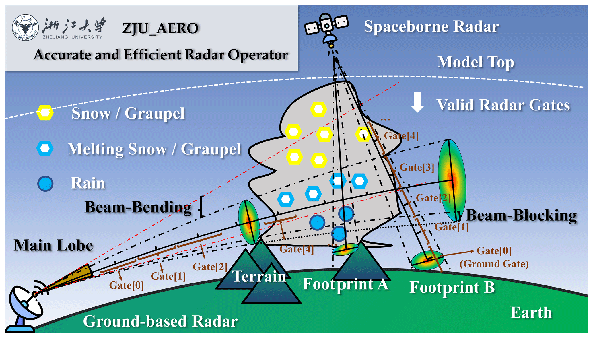
Figure 1 A conceptual graph illustrating the types of simulations that the Accurate and Efficient Radar Operator designed by ZheJiang University (ZJU-AERO) can accommodate. This graph visualizes the beam-bending and beam-blocking effects, which are taken into considerations by many radar operators designed for ground-based radars. For these radars, the sampling volume within the main lobe of the radar antenna patterns increases with the range of detection, as indicated by the area between the two dashed–dotted black curves. The radar beam follows a $\mathrm{4}/\mathrm{3}{R}_{\mathrm{E}}$ radius curve under standard atmospheric profile conditions and is commonly referred to as beam-bending (in which R_E is the radius of the Earth). Note that the sampling volume can be partially blocked by terrain, as indicated by the area above the dotted black line. The spaceborne radar scans, which have relatively small zenith angles (usually within 20°), are weakly affected by the beam-bending phenomenon. The radar gates of ground-based radar are recorded from the zero-range bin, while the gates of spaceborne radar are only stored within the data sampling range with respect to mean sea level; for example, GPM/DPR products only stores range bins at altitudes between −5 and 19 km, as spaceborne radars scan always cast a footprint on the Earth. In ZJU-AERO, only the radar gates beneath the NWP model top, known as “valid radar gates”, are represented and simulated in order to save on memory usage and computational resources.

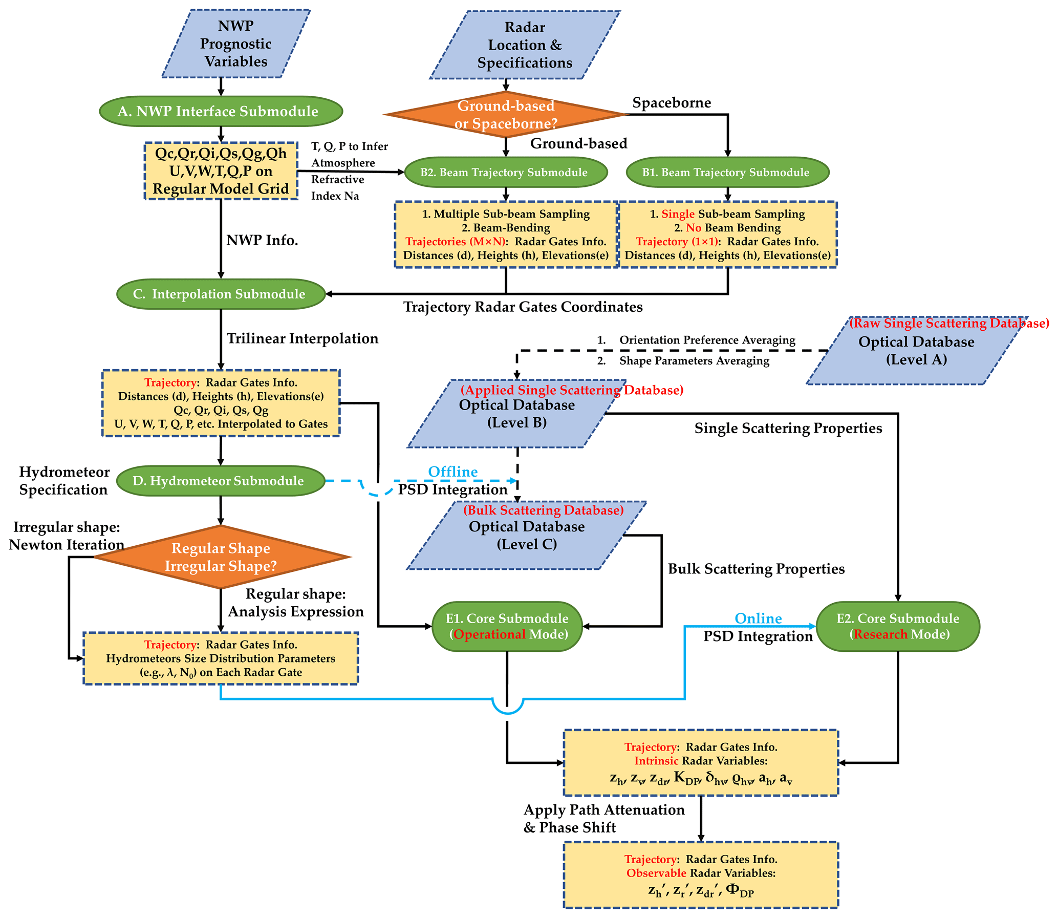
Figure 2 A conceptual flowchart of ZJU-AERO. The parallelogram boxes represent input data (including numerical weather prediction (NWP) output, radar specifications, and optical property lookup tables). The round green rectangles indicate the names of the key submodules of ZJU-AERO. The dashed yellow boxes indicate the key data structure used in the simulations. The diamonds represent the points at which crucial “if–else” judgments can be conducted during processing. Those dashed arrows in this flowchart represent external database generation steps carried out using the released tool scripts of ZJU-AERO.

2.1 Flowchart and concepts

Figure 2 provides an overview of the ZJU-AERO simulation procedure for a single-radar scan. ZJU-AERO consists of five modules represented by green boxes in Fig. 2. These modules are the (A) NWP interface submodule, (B) beam submodule (decomposed into B1 and B2 for ground-based and spaceborne radars, respectively, (C) interpolation submodules, (D) hydrometeor submodule, and (E) core submodule. The workflow of ZJU-AERO can be summarized as follows:

• 1.

  The NWP interface submodule (A) reads NWP prognostic variables from external storage files and interpolates the data defined on the original model grid (such as horizontal Arakawa-C grid and vertical Charney–Phillips grid in CMA–GFS/MESO; Chen et al., 2008; Shen et al., 2023) to a regular grid on which all variables are co-located and evenly spaced horizontally (in the space of projection). The prognostic variables include hydrometeor variables (Q_c, Q_i, Q_r, Q_s, and Q_g, representing the mixing ratios of cloud water, cloud ice, rain, snow, and graupel, respectively) and dynamic variables (U, V, W, T, P, and Q, representing the zonal, meridional, vertical wind, temperature, pressure, and water vapor mixing ratio, respectively). Additionally, static model information such as orography data defined on model grids is required for simulating partial beam blocking. This step prepares for a quick and convenient second-round interpolation from the regular model grid to the radar beam trajectories (in step 3). It is worth pointing out that ZJU-AERO can also interface with the output of WRF NWP model (Skamarock et al., 2019). Enabling ZJU-AERO to interface with grid data from another NWP model involves only technical adjustments that require basic information about that NWP model's horizontal mesh (projections), vertical grid, and variable mapping table.

• 2.

  The beam trajectory submodule (B) calculates the propagation trajectories of the radar beam. For ground-based radar (B1), users have the option of using an online trajectory solver that uses temperature and humidity profiles above the radar site. Specifically, the atmosphere refractive index Na are determined from atmosphere temperature T, pressure P, and water vapor mixing ratio Q. The trajectory is determined by a ray-tracing ordinary differential equation (ODE) solver (Zeng et al., 2014). Additionally, ZJU-AERO offers an alternative option of using an offline $\mathrm{4}/\mathrm{3}{R}_{\mathrm{E}}$ solver for ground-based radar in ZJU-AERO. Multiple sub-trajectories (determined by the horizontal quadrature number N × vertical quadrature number M) are sampled within the 3 dB beamwidth of the main lobe for the N × M sub-trajectories. The observable radar variables are calculated by integrating bulk-scattering properties over the antenna patterns (as described in step 5) to obtain the final results (beam-broadening and beam-blocking are considered in this way). We applied the sub-beam sampling and averaging methods described in Zeng et al. (2016). Nevertheless, for spaceborne radar (B2), the beam trajectory is computed using the geometry shown in Fig. A1, and sub-trajectory averaging is not supported at this time. For more details on the beam trajectory module of spaceborne radar (B2), please refer to Appendix A.

• 3.

  The interpolation submodule (C) uses a trilinear interpolation algorithm to interpolate the NWP prognostic variables to the gates of radar beam trajectories. The quick trilinear interpolations are performed in a two-step manner: (1) vertically interpolating the data defined on the eight vertices of the cube containing the radar gates to the four vertices of the horizontal box surrounding the radar gate and (2) performing bilinear interpolation; we adopted the approach described in Appendix A of Wolfensberger and Berne (2018) and reimplemented it as a Cython extension.

• 4.

  The hydrometeor submodule (D) specifies the properties of hydrometeors in each radar gate along each trajectory, usually by loading presets of microphysics-consistent constants of hydrometeors. This includes the orientation preference, probability distribution of particle morphology, particle size distribution (PSD), and other parameters. Those presets of hydrometeor properties can also be modified by users to perform “forced” (i.e., inconsistent with microphysics) simulations for research purposes. The PSD parameters of hydrometeors are solved in this step from prognostic bulk-hydrometeor variables in NWP models (mass concentrations and number concentrations). For more details, see Sect. 2.3.

• 5.

  The core module (E) finally calculates the polarimetric radar variables.

  • 5.1

    The bulk-scattering properties of particles in each radar gate are computed by integrating the single-scattering properties across the size spectrum of each hydrometeor type and summing over hydrometeor types, which can be conducted either online (E1; research mode) or offline (E2; operational mode) in ZJU-AERO. The scattering property LUTs of ZJU-AERO are consulted in this step, which is composed of three levels (level A, level B, and level C). The multi-layered architecture will be introduced in detail in Sect. 3.1. The research mode is more flexible since it accesses the level B database for single-scattering property, while the operational mode is more efficient by accessing the level C database for bulk-scattering properties straightforward. We provide users with tool scripts for level A to B and level B to C conversions (integration parameters are alterable in YAML configure files).

  • 5.2

    Once the bulk-scattering properties on each sub-trajectory grid point within each radar gate are available, the antenna pattern integration involves integrating the bulk-scattering properties within the scanning volume of each radar gate.

  • 5.3

    Then, the core module calculates the intrinsic polarimetric radar variables on each radar gate, based on the bulk-scattering properties incorporating the antenna pattern integration presented in step 5.2. These radar variables include single-polarization reflectivities (Z_H for horizontal reflectivities), dual-polarization variables (Z_DR, K_DP, δ_hv, Φ_DP, and ρ_hv for differential reflectivity, differential phase shift, backscatter differential phase, and co-polar correlation coefficient, respectively), and attenuation variables (a_H and a_V for horizontal and vertical attenuation coefficients, respectively). The definitions of these variables can be found in Appendix D. For a detailed explanation of the intrinsic radar variables, please refer to Zhang (2016).

  • 5.4

    In the final step of core module, the observable radar variables are obtained by taking into account the attenuation and phase shift accumulated along the beam trajectories.

The above procedures of steps 2–5 are independent for each single beam, which guarantees the top-level scalability of the forward operator. Therefore, we are using the shared-memory Python parallel library (multiprocessing) to speed up the simulation.

In addition, for those computationally intensive tasks (such as the trilinear interpolation in step 3), we are employing the technique of mixed programming (building C/Fortran extensions that interface with Python scripts) to further accelerate the computation.

The performance of the forward operator is generally satisfactory; ZJU-AERO can complete a ground-based station volume scan with nine plan position indicator (PPI) sweeps in 2 min on a modern laptop CPU with a six-core processor (i7-10750H) if the online size distribution integration is performed and the operator takes the level B single-scattering property database as input. If the level C bulk-scattering property database is used, such a volume PPI scan can be completed even faster (in 30 s). Such efficiency can support data assimilation purposes while also preserving flexibility for research purposes.

In this paper, we do not elaborate on the algorithm details of certain issues, such as (a) trilinear interpolation, (b) sub-beam sampling and antenna-pattern-weighted averaging, and (c) a ray-tracing trajectory solver. For trilinear interpolation, we follow the approach described in Wolfensberger and Berne (2018) to interpolate the model grid data to the radar gates of each sub-trajectory grid point. Regarding sub-beam sampling and antenna-pattern-weighted averaging, we utilized Gauss–Hermite quadrature, as outlined in Caumont et al. (2006). As the ray-tracing trajectory solver, we offer users both an offline beam trajectory solver ($\mathrm{4}/\mathrm{3}{R}_{\mathrm{E}}$) and an online beam trajectory solver (Zeng et al., 2014). All of these methods are reimplemented in Python using either efficient NumPy/SciPy API or customized Cython extensions.

2.2 Physical basis

At this point, we can specify the formulation convention used in the radar operator and move on to the non-spherical optical database design of ZJU-AERO.

The amplitude-scattering matrix S_FSA of a single particle is defined as follows:

$$\begin{array}{}\text{(1)}& \begin{array}{rl}\left[\begin{array}{l}{E}_{\mathrm{h}}^{\mathrm{sca}}\\ E_{\mathrm{v}}^{\mathrm{sca}}\end{array}\right]& ={\displaystyle \frac{e^{-i{k}_{\mathrm{0}}r}}{r}}{\mathbf{S}}_{\mathrm{FSA}}\left[\begin{array}{l}{E}_{\mathrm{h}}^{\mathrm{inc}}\\ E_{\mathrm{v}}^{\mathrm{inc}}\end{array}\right]\\ & ={\displaystyle \frac{e^{-i{k}_{\mathrm{0}}r}}{r}}{\left[\begin{array}{ll}{S}_{\mathrm{hh}}& S_{\mathrm{hv}}\\ S_{\mathrm{vh}}& S_{\mathrm{vv}}\end{array}\right]}_{\mathrm{FSA}}\left[\begin{array}{l}{E}_{\mathrm{h}}^{\mathrm{inc}}\\ E_{\mathrm{v}}^{\mathrm{inc}}\end{array}\right].\end{array}\end{array}$$

In Eq. (1), E indicates the vector electric field, and the superscripts “sca” and “inc” represent scattering and incident waves, respectively. The subscripts “h” and “v” indicate two decomposed components of the vector electric field in the horizontal and vertical directions, respectively. Specifically, the horizontal and vertical unit vectors are defined as unit vectors, $\widehat{\mathit{\varphi }}$ and $\widehat{\mathit{\theta }}$, of the spherical coordinate system under the forward scattering alignment (FSA) convention. The differences between FSA and backward-scattering alignment (BSA) are described in Appendix C. k₀ is the wave number in free space, and r is the distance from the particle center.

The scattering matrix relates the incident electric field to the scattered electric field, and it must have the dimension of L (L is the dimension symbol of length). In practice, the amplitude-scattering matrix is usually expressed in the units of millimeters. The amplitude-scattering matrix of a single hydrometeor particle is obtained from scattering computations, specifically using the T-matrix method in this study.

Apart from the 2 × 2 complex amplitude-scattering matrix S defined on complex electric field vector bases, one can define the 4 × 4 real matrix, known as the Mueller matrix, Z, and extinction matrix, K, which describe polarimetric light-scattering and extinction properties of particles on the real Stokes vector bases, respectively. We kept the definitions of Z and K consistent with those mentioned in a study by Mishchenko (2014).

The Mueller and extinction matrices can be derived from the amplitude-scattering matrix (Mishchenko, 2014). Specifically, the forward amplitude-scattering matrix shows a linear relationship with K. For example, the formulas of the matrix elements of K used in this study are shown below:

$$\begin{array}{}\text{(2)}& \begin{array}{l}{K}_{\mathrm{11}}=\frac{\mathrm{2}\mathit{\pi }}{k_{\mathrm{0}}}\mathfrak{I}(S_{\mathrm{hh}}+S_{\mathrm{vv}}).\\ K_{\mathrm{12}}=\frac{\mathrm{2}\mathit{\pi }}{k_{\mathrm{0}}}\mathfrak{I}(S_{\mathrm{hh}}-S_{\mathrm{vv}}).\\ K_{\mathrm{34}}=\frac{\mathrm{2}\mathit{\pi }}{k_{\mathrm{0}}}\mathfrak{R}(S_{\mathrm{vv}}-S_{\mathrm{hh}}).\end{array}\end{array}$$

Here, the notations of ℑ and ℜ indicate the real and imaginary parts of a complex number, respectively. On the other hand, the backscattering-amplitude matrix can be used to calculate Z in backscattering geometry. For example, the formulas of the matrix elements of Z used in this study are shown below:

$$\begin{array}{}\text{(3)}& \begin{array}{l}{Z}_{\mathrm{11}}=\frac{\mathrm{1}}{\mathrm{2}}\left({\left|S_{\mathrm{hh}}\right|}^{\mathrm{2}}+{\left|S_{\mathrm{hv}}\right|}^{\mathrm{2}}+{\left|S_{\mathrm{vh}}\right|}^{\mathrm{2}}+{\left|S_{\mathrm{vv}}\right|}^{\mathrm{2}}\right).\\ Z_{\mathrm{12}}=\frac{\mathrm{1}}{\mathrm{2}}\left({\left|S_{\mathrm{hh}}\right|}^{\mathrm{2}}-{\left|S_{\mathrm{hv}}\right|}^{\mathrm{2}}+{\left|S_{\mathrm{vh}}\right|}^{\mathrm{2}}+{\left|S_{\mathrm{vv}}\right|}^{\mathrm{2}}\right).\\ Z_{\mathrm{21}}=\frac{\mathrm{1}}{\mathrm{2}}\left({\left|S_{\mathrm{hh}}\right|}^{\mathrm{2}}+{\left|S_{\mathrm{hv}}\right|}^{\mathrm{2}}-{\left|S_{\mathrm{vh}}\right|}^{\mathrm{2}}-{\left|S_{\mathrm{vv}}\right|}^{\mathrm{2}}\right).\\ Z_{\mathrm{12}}=\frac{\mathrm{1}}{\mathrm{2}}\left({\left|S_{\mathrm{hh}}\right|}^{\mathrm{2}}+{\left|S_{\mathrm{hv}}\right|}^{\mathrm{2}}+{\left|S_{\mathrm{vh}}\right|}^{\mathrm{2}}+{\left|S_{\mathrm{vv}}\right|}^{\mathrm{2}}\right).\\ Z_{\mathrm{22}}=\frac{\mathrm{1}}{\mathrm{2}}\left({\left|S_{\mathrm{hh}}\right|}^{\mathrm{2}}-{\left|S_{\mathrm{hv}}\right|}^{\mathrm{2}}-{\left|S_{\mathrm{vh}}\right|}^{\mathrm{2}}+{\left|S_{\mathrm{vv}}\right|}^{\mathrm{2}}\right).\\ Z_{\mathrm{33}}=\mathfrak{R}\left(S_{\mathrm{hh}}{S}_{\mathrm{vv}}^{\ast }+S_{\mathrm{hv}}{S}_{\mathrm{vh}}^{\ast }\right).\\ Z_{\mathrm{34}}=\mathfrak{I}\left(S_{\mathrm{hh}}{S}_{\mathrm{vv}}^{\ast }+S_{\mathrm{vh}}{S}_{\mathrm{hv}}^{\ast }\right).\\ Z_{\mathrm{43}}=\mathfrak{I}\left(S_{\mathrm{vv}}{S}_{\mathrm{hh}}^{\ast }-S_{\mathrm{hv}}{S}_{\mathrm{vh}}^{\ast }\right).\\ Z_{\mathrm{44}}=\mathfrak{R}\left(S_{\mathrm{vv}}{S}_{\mathrm{hh}}^{\ast }-S_{\mathrm{hv}}{S}_{\mathrm{vh}}^{\ast }\right).\end{array}\end{array}$$

The complete set of equations from the elements of the amplitude matrix S to each element of the Mueller matrix Z or the extinction matrix K can be found in Mishchenko (2014). The elements of Z and K are both in the dimension of L² (i.e., they are usually expressed in the units of mm²).

We could compute the bulk-scattering properties 〈X〉¹ used in the expression of several polarimetric radar variables by performing size distribution integrations over elements of Z and K matrices:

$$\begin{array}{}\text{(4)}& 〈\mathit{X}〉={\int }_{\mathrm{0}}^{\mathrm{\infty }}\mathit{X}\left(D\right)N\left(D\right)\mathrm{d}D,\mathit{X}=\mathbf{Z},\mathbf{K}.\end{array}$$

Here, N(D) represents the number concentration distribution function (in units of mm⁻¹ m⁻³) over the particle spectrum, and D is the diameter² of the hydrometeor (in units of mm). The elements of bulk matrices 〈Z〉 and 〈K〉 were usually expressed in units (of mm² m⁻³).

Note that we can only apply the particle ensemble integration over the complex amplitude-scattering matrix, S, in the forward scattering geometry. This is because integrating over extinction matrix elements is proportional to integrating corresponding forward amplitude-scattering matrix elements. For example:

$$\begin{array}{}\text{(5)}& 〈K_{\mathrm{11}}〉={\displaystyle \frac{\mathrm{2}\mathit{\pi }}{k_{\mathrm{0}}}}〈S_{\mathrm{hh}}〉+{\displaystyle \frac{\mathrm{2}\mathit{\pi }}{k_{\mathrm{0}}}}〈S_{\mathrm{vv}}〉.\end{array}$$

Equation (5) is derived by performing ensemble mean on Eq. (2).

Therefore, we use Mueller and extinction matrices to represent radar variables because ensemble means can be performed directly on them, as is not the case for amplitude matrix. Also, they have a unified dimension of L². The LUTs in ZJU-AERO store Mueller and extinction matrices instead of the amplitude matrix (see Appendix B, which will be further described in Sect. 3.1). The equations for radar variables based on Mueller and extinction matrices can be found in Appendix D.

2.3 Hydrometeor specifications

Table 1 summarizes the hydrometeor specifications in ZJU-AERO, with the following important notes:

1. During the early-development stage of ZJU-AERO, we initially used the dielectric model for water proposed by Liebe et al. (1991). However, we transitioned to a more accurate and contemporary dielectric model developed by Ellison (2007). Nevertheless, we retained the outdated option and optical property lookup table from the old dielectric model in our archive for future reference and comparison (see the column of the refractive index model in Table 1).

2. In principle, it is encouraged to use PSD schemes compatible with the microphysics package in the NWP model to ensure consistent hydrometeor settings in simulations. Therefore, ZJU-AERO, which is designed for CMA–GFS/MESO, provides PSD options that are compatible with the single-moment microphysics scheme WSM6 (Hong and Lim, 2006) and Thompson (Thompson et al., 2008), which are widely used in the global and regional operational models of CMA. For instance, option C1 for rain and option B1 for graupel are compatible with the WSM6 package, while option C2 for rain and option B2 for graupel are compatible with the Thompson package (see the column of particle size distribution in Table 1). However, for the snow category, we implemented the PSD scheme of Field et al. (2005) as the only option since it is the widely acknowledged as the best globally applicable temperature-dependent PSD model for solid precipitation. Additionally, we have provided users with some additional PSD schemes for sensitivity assessment, such as options C3 (Wang et al., 2016) and C4 (Abel and Boutle, 2012) for the rain category. Those PSD schemes in the ZJU-AERO that are incompatible with the microphysics package used in the NWP model are referred to as forced PSD schemes.

3. Solid hydrometeor categories, such as snow and graupel, are known to have relatively larger uncertainties associated with parameterizations of aspect ratios and orientation preference. To address these uncertainties, a field research study conducted by Garrett et al. (2012) used an in situ observation instrument called the multi-angle snowflake camera (MASC). This instrument was used to measure the aspect ratios and orientations of over 30 000 solid particles in the eastern Swiss Alps. The particles were then classified into aggregates (corresponding to the snow category in this study), rimed particles, and graupel, as described in Garrett et al. (2015). The fitted model from this study was used as a priori knowledge of hydrometeor shape specifications in the ZJU-AERO (see the column of shape parameters in Table 1):

   $$\begin{array}{}\text{(6)}& p(\mathit{\gamma };D_{\max })\propto {\left(\mathit{\gamma }-\mathrm{1}\right)}^{K\left(D_{\max }\right)-\mathrm{1}}\exp \left(-{\displaystyle \frac{\mathit{\gamma }-\mathrm{1}}{\mathrm{\Theta }\left(D_{\max }\right)}}\right).\end{array}$$

   Equation (6) provides the probability distribution function of the aspect ratio in which γ is the reciprocal of the aspect ratio (minor axis/major axis, always less than unity). It is assumed to follow a gamma distribution with an offset coefficient of 1 (i.e., γ>1). The shape coefficient, K(D_max), and a scale coefficient, Θ(D_max), are functions of the particle maximum dimension. We used the power law relationships of K(D_max) and Θ(D_max) that were fitted by Wolfensberger and Berne (2018) as follows:

   $$\begin{array}{}\text{(7)}& \begin{array}{l}{K}_{\mathrm{snow}}\left(D_{\max }\right)=\mathrm{8.42}{D}_{\max }^{-\mathrm{0.57}};{\mathrm{\Theta }}_{\mathrm{snow}}\left(D_{\max }\right)\\ =\mathrm{0.053}{D}_{\max }^{-\mathrm{0.79}}.\\ K_{\mathrm{graupel}}\left(D_{\max }\right)=\mathrm{3.2}{D}_{\max }^{-\mathrm{0.42}};{\mathrm{\Theta }}_{\mathrm{graupel}}\left(D_{\max }\right)\\ =\mathrm{0.074}{D}_{\max }^{-\mathrm{0.67}}.\end{array}\end{array}$$

4. Since solving the PSD parameters from NWP prognostic hydrometeor mass concentrations (for bulk microphysics) requires knowledge of the mass of various particle sizes, the mass–diameter relationship is crucial in determining the PSD (see the column of mass–diameter relationship in Table 1). In this study, all the hydrometeor categories follow the gamma distribution (the widely used exponential distribution is just a special case of gamma distribution when μ=1),

   $$\begin{array}{}\text{(8)}& N\left(D\right)=N_{\mathrm{0}}{D}^{\mathit{\mu }}{e}^{-\mathrm{\Lambda }D},\end{array}$$

   in which N₀ is the intercept, Λ is the slope, and μ is the shape coefficient of that gamma distribution. As is often the case (for all PSD options in ZJU-AERO; see Table 1), μ is a prescribed constant in the microphysics package, while N₀ either equals a prescribed constant or relates to Λ by a power law in which x₁ and x₂ are parameters fitted by drop size distribution (DSD) observations (see Sect. 3.4):

   $$\begin{array}{}\text{(9)}& N_{\mathrm{0}}=x_{\mathrm{1}}{\mathrm{\Lambda }}^{x_{\mathrm{2}}}.\end{array}$$

   If a hydrometeor category is of a single-moment microphysics scheme, given the mass concentration of arbitrary hydrometeor category “x” Q_x (in units of kg m⁻³),

   $$\begin{array}{}\text{(10)}& Q_x=\underset{\mathrm{0}}{\overset{\mathrm{\infty }}{\int }}\stackrel{\mathrm{‾}}{m}\left(D\right)\cdot N\left(D\right)\mathrm{d}D.\end{array}$$

   If the mass–diameter relationship can be approximated as a power law form $\stackrel{\mathrm{‾}}{m}\left(D\right)=a{D}^b$ in which $\stackrel{\mathrm{‾}}{m}\left(D\right)$ is the average mass of a given size of a particle (considering that some hydrometeor categories have a probability distribution over shape parameters such as aspect ratio). Then we can solve the unknown parameter Λ and determine all relevant PSD information that pertains to that radar gate analytically by plugging Eq. (8) into Eq. (10) as follows:

   $$\begin{array}{}\text{(11)}& \mathrm{\Lambda }={\left[{\displaystyle \frac{a{x}_{\mathrm{1}}\mathrm{\Gamma }(\mathrm{1}+b+\mathit{\mu })}{Q_x}}\right]}^{\frac{\mathrm{1}}{\mathrm{1}+b+\mathit{\mu }-x_{\mathrm{2}}}}.\end{array}$$

   Again, there is a microphysics-consistent mass–diameter relationship $\stackrel{\mathrm{‾}}{m}\left(D_{\max }\right)=\frac{\mathit{\pi }}{\mathrm{6}}{\mathit{\rho }}_{\mathrm{sp}}{D}_{\max }^{\mathrm{3}}({\mathit{\rho }}_{\mathrm{sp}}$ is the overall density of the solid precipitation sphere particle) for snow and graupel. Many microphysics schemes, such as WSM6, simply treated solid precipitation categories as spheres with different ice–air mixture ratios and hence different overall densities ρ_sp. However, this practice can result in a huge inconsistency between the mass concentration represented by radar operators and the microphysics schemes since the actual average mass of a given size bin is represented by the following probability-weighted averaging over the aspect ratio for solid hydrometeors shown below:

   $$\begin{array}{}\text{(12)}& \stackrel{\mathrm{‾}}{m}\left(D_{\max }\right)=\underset{\mathrm{1}}{\overset{\mathrm{\infty }}{\int }}p(\mathit{\gamma };D_{\max })m(\mathit{\gamma };D_{\max })\mathrm{d}\mathit{\gamma }.\end{array}$$

   It turns out that fitting Eq. (12) into power laws is troublesome when the probability distribution function p(γ;D_max) varied dramatically with diameter. This problem will become even worse when we introduce other non-spherical particles, such as snowflakes.

   To resolve this error when using a traditional mass–diameter relationship, we implemented a benchmark PSD solver employing a numerical method (i.e., Newton iteration) for particles with complicated morphology specifications. The simplest case, a PSD represented by an exponential distribution with a fixed intercept parameter N₀, can be used as an example. Here the equation for the unknown PSD parameter Λ can be expressed as follows:

   $$\begin{array}{}\text{(13)}& \begin{array}{rl}{Q}_x& =\sum _{D_i=D_{\mathrm{l}}}^{D_i=D_{\mathrm{u}}}\stackrel{\mathrm{‾}}{m}\left(D_i\right)N\left(D_i\right)\mathrm{\Delta }D\\ & =\sum _{D_i=D_{\mathrm{l}}}^{D_i=D_{\mathrm{u}}}\stackrel{\mathrm{‾}}{m}\left(D_i\right)N_{\mathrm{0}}{e}^{-\mathrm{\Lambda }{D}_i}\mathrm{\Delta }D,\end{array}\end{array}$$

   in which the integration in Eq. (10) is truncated within a specific diameter range of [D_l,D_u] and further discretized as a summation. The expression of the exponential distribution is then substituted in for the second equality. $\stackrel{\mathrm{‾}}{m}\left(D_i\right)$ at discretized size bins is precomputed by Eq. (12) and treated as a constant. The mass m(γ;D_i) for each morphology specification can be calculated as the density of the pure ice ρ_ice multiplied by the volume occupied by the non-spherical hydrometeor particle model V(γ;D_i) (calculated from mathematical formulas of geometrical bodies).

   We then define the function F(Λ) and its derivative F^′(Λ) in the Newton iteration as follows:

   $$\begin{array}{}\text{(14)}& \begin{array}{l}F\left(\mathrm{\Lambda }\right)=\sum _{D_i=D_{\mathrm{l}}}^{D_i=D_{\mathrm{u}}}\stackrel{\mathrm{‾}}{m}\left(D_i\right)N_{\mathrm{0}}{e}^{-\mathrm{\Lambda }{D}_i}\mathrm{\Delta }D-Q_x,\\ F^{\prime }\left(\mathrm{\Lambda }\right)=-\sum _{D_i=D_{\mathrm{l}}}^{D_i=D_{\mathrm{u}}}\stackrel{\mathrm{‾}}{m}\left(D_i\right)N_{\mathrm{0}}{e}^{-\mathrm{\Lambda }{D}_i}{D}_i\mathrm{\Delta }D.\end{array}\end{array}$$

   Based on the above formulation, the iteration relationship to derive the (n+1)th guess Λ_n+1 from the nth guess Λ_n can be expressed as shown below:

   $$\begin{array}{}\text{(15)}& {\mathrm{\Lambda }}_{n+\mathrm{1}}={\mathrm{\Lambda }}_n-{\displaystyle \frac{F\left({\mathrm{\Lambda }}_n\right)}{F^{\prime }\left({\mathrm{\Lambda }}_n\right)}}.\end{array}$$

   While performing iterations online (the benchmark PSD solver) may lead to a decrease in the efficiency of the ZJU-AERO, this problem can be resolved using bulk-scattering property (BSP) LUTs instead of single-scattering property (SSP) LUTs (see Sect. 3.5).

Table 1 An overview of the specification for all categories of hydrometeors in the Accurate and Efficient Radar Operator designed by ZheJiang University (ZJU-AERO). Some sophisticated specifications are only tagged with a bibliography and explained with more detail of the context to make this table more compact and convenient for reference.

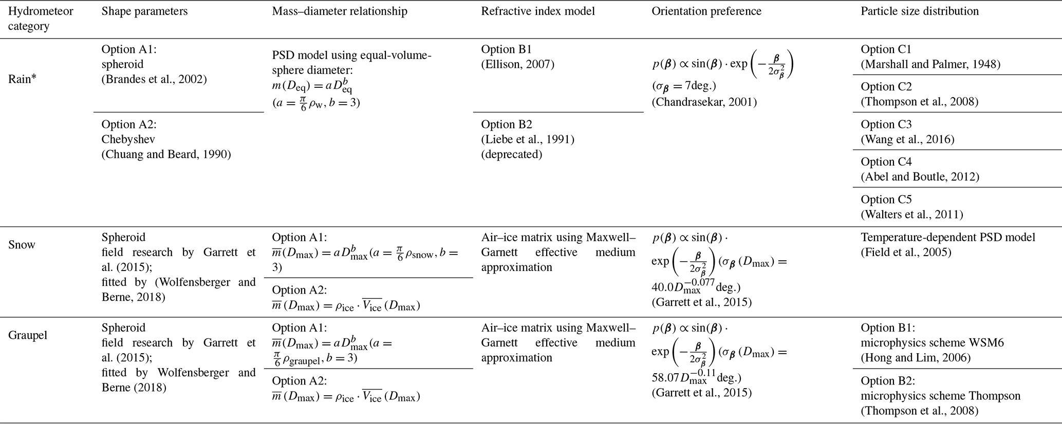
^* The specifications regarding the hydrometeor category of rain are discussed in Sect. 3.

3 Database of hydrometeor optical properties

In Sect. 2, we provide a comprehensive description of the design of ZJU-AERO. Specifically, we emphasize that the hydrometeor optical property database includes the elements of Z and K (in units of mm²) for single-scattering properties and those of 〈Z〉 and 〈K〉 (in units of mm² m⁻³) for bulk-scattering properties, both in the FSA convention. In the first two subsections, we will delve into the design of the database (LUT) in ZJU-AERO with more details.

Furthermore, ZJU-AERO currently encompasses three types of hydrometeors: (1) rain, (2) snow, and (3) graupel. Among these hydrometeors, the rain category offers a non-spherical shape parameter option, known as the Chebyshev shape. This shape differs from the traditional spheroid shape commonly used in other radar observation operators. Therefore, we will evaluate the database contents using the Chebyshev raindrop as an example in the last three subsections.

3.1 The multi-layered architecture

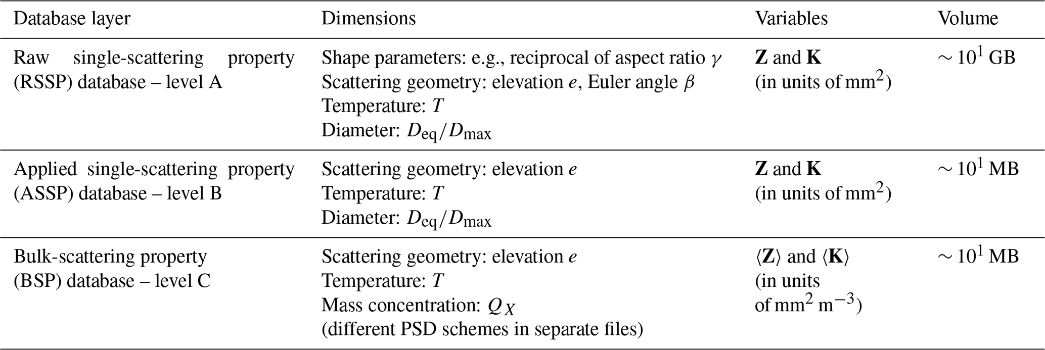
The ZJU-AERO optical property database is designed with a multi-layered architecture consisting of three levels: (1) the raw single-scattering property (RSSP) database (level A), (2) the applied single-scattering property (ASSP) database (level B), and (3) the BSP database (level C). These levels are described in detail in Table 2.

The RSSP level A database contains the optical properties of individual particles without any averaging or integration over the shape parameters and orientations, which normally consumed a significant amount of memory resources (∼ 10¹ GB). However, using the RSSP in ZJU-AERO would require the online integration of orientations and shape parameters, leading to a significant slow-down in radar operator performance. On the other hand, if shape and orientation averaging were applied during the creation of the database, and the raw optical data (RSSP) are discarded, then the resulting database would lack the flexibility needed for modifying the shape and orientation distributions. Additionally, future enhancements to the ZJU-AERO database may involve incorporating more sophisticated shape parameters for the non-spherical hydrometeors. Therefore, retaining the RSSP level A database is essential to accommodate uncertainties and increase the convenience in experiments and simulations related to shape and orientation parameters.

Building on the RSSP level A database, the ASSP level B database improves the computational efficiency by carrying out averaging or orientation over shape parameters and orientations offline. Finally, the BSP level C optical database integrates the optical properties stored in the ASSP level B database over PSD and enables fast batch running in ZJU-AERO for operational use. In summary, the multi-layered architecture of the lookup table (stored in netCDF4 format files separately for different database levels) is to strike a balance between the flexibility of the database and the computational efficiency required by radar operators. Future releases of ZJU-AERO will provide software tools for flexible conversions between the database levels, allowing users to easily configure integration parameters.

Table 2 The architectural design of the multi-layered hydrometeor optical properties database used in ZJU-AERO. The column “Volume” gives an estimation of the external storage that a single-database lookup table file for one hydrometeor class and one frequency occupies. Note that only the order of magnitude of storage space is shown in those entries. The grids of dimensions in this table can be found in Table B1 of Appendix B.

3.2 Scattering geometry

Figure 3 depicts the Cartesian coordinate system used to determine the scattering geometry of a hexagonal plate particle. The laboratory coordinate system, denoted as OX_LY_LZ_L, is aligned by vertically positioning its OZ_L axis and placing its OX_L axis in the vertical plane specified by the incident radar beam and OZ_L. This alignment sets the azimuthal angle ϕ_inc of the radar beam to zero. In Fig. 3a, the direction of the radar beam is shown, which is practically specified using the elevation angle $e\in \left[-\mathit{\pi }/\mathrm{2},\mathit{\pi }/\mathrm{2}\right]$. For ground-based radar, this angle is positive, while for spaceborne radar, it is negative. In this context, the polar angle of the radar beam, denoted as θ_inc, is related to the elevation angle through ${\mathit{\theta }}_{\mathrm{inc}}=\mathit{\pi }/\mathrm{2}-e$. The shape of the particle is defined in the particle coordinate system OX_PY_PZ_P. In the specific example shown in Fig. 3d, the OZ_P axis is set perpendicular to the basal face of a hexagonal plate. The origin “O” is placed at the mass center of the particle, and the OY_P axis intersected two opposite vertices of the hexagonal basal face. Using the ZYZ convention of the Euler angles specified by α, β, and γ (rotations were performed with respect to the OZ_P, OY_P, and OZ_P axes, respectively), any arbitrary orientation of a given particle can uniquely be determined (see Fig. 3b–d).

With a specified scattering geometry, we can now outline the procedures for computing the scattering properties of particles with fixed orientations (steps 1–3) and then integrate over them for scattering properties with specific orientation preference (step 4):

1. We used the T-matrix method to compute the T-matrix only once for a given particle and a radar beam wavelength. The guidelines for selecting a scattering computation approach are as follows: for both axially symmetric (i.e., the dielectric constant distribution of electromagnetic medium in spherical coordinates ε(rθφ) is irrelevant with azimuth angle φ) and homogenous particles, we used the EBCM T-matrix code (Mishchenko and Travis, 1994), while for particles without axial symmetry or those that are inhomogeneous (or shapes for which the EBCM approach suffers from numerical stability issues), we applied the invariant-imbedding T-matrix (IITM) code (Bi et al., 2013; Bi and Yang, 2014; Bi et al., 2022; Wang et al., 2023).

2. With the T-matrix computed in Step 1, we efficiently calculated the forward and backward-amplitude-scattering matrix S_FSAin Eq. (1) for tuples of scattering geometry (α, β, γ, and e), using the method of Mishchenko (2000).

3. The forward and backward-amplitude-scattering matrices S_FSA were then converted into the backscattering Mueller and extinction matrices, Z and K, respectively (Mishchenko, 2014).

4. When averaging over α and γ, we considered that the atmosphere is generally horizontally isotropic on the scale of hydrometeor particles. It is believed that they should have no preference for Euler angles α and γ, except for extreme conditions such as the lightening-induced reorientation of ice crystals (Hubbert et al., 2010). Therefore, we performed internal averaging over α and γ for elements of Z and K in the scattering-computation code before generating the RSSP level A database:

   $$\begin{array}{}\text{(16)}& \stackrel{\mathrm{‾}}{\mathbf{X}}(e,\mathit{\beta })={\displaystyle \frac{\mathrm{1}}{\mathrm{4}{\mathit{\pi }}^{\mathrm{2}}}}\underset{\mathrm{0}}{\overset{\mathrm{2}\mathit{\pi }}{\int }}\mathrm{d}\mathit{\alpha }\underset{\mathrm{0}}{\overset{\mathrm{2}\mathit{\pi }}{\int }}\mathrm{d}\mathit{\gamma }\mathbf{X}(e,\mathit{\alpha },\mathit{\beta },\mathit{\gamma }),\mathbf{X}=\mathbf{Z},\mathbf{K}.\end{array}$$

   ³Hence, the level A database only has two residual scattering geometry dimensions: (1) e and (2) β, allowing for a reasonable volume for archiving.

   The integration in the level A to level B database conversion tool can be formalized as the integration over the canting angle β as follows:

   $$\begin{array}{}\text{(17)}& \stackrel{\mathrm{‾}}{\stackrel{\mathrm{‾}}{\mathit{X}}}\left(e\right)={\displaystyle \frac{\mathrm{1}}{\mathit{\pi }}}\underset{\mathrm{0}}{\overset{\mathit{\pi }}{\int }}\sin \left(\mathit{\beta }\right)\mathrm{d}\mathit{\beta }p\left(\mathit{\beta }\right)\stackrel{\mathrm{‾}}{\mathit{X}}(e,\mathit{\beta }),\mathit{X}=\mathbf{Z},\mathbf{K}.\end{array}$$

   ⁴Here p(β) is the probability distribution of canting angle β. A Gaussian distribution in the polar angle is often used to approximate the probability distribution of canting angle,

   $$\begin{array}{}\text{(18)}& p\left(\mathit{\beta }\right)=\exp \left(-{\displaystyle \frac{\mathit{\beta }}{\mathrm{2}{\mathit{\sigma }}_{\mathit{\beta }}^{\mathrm{2}}}}\right).\end{array}$$

   Here the standard deviation of canting angle, σ_β, can be found in the orientation preference column in Table 1.

   Particle symmetry can be considered in the orientation averaging of Eqs. (16) and (17) to avoid a redundant evaluation of Z and K. For example, in the case of a hexagonal plate with an 6-fold azimuthal symmetry and xy-plane reflectance symmetry, Z and K only need to be evaluated and averaged over $\mathit{\alpha }\in \left[\mathrm{0},\mathit{\pi }/\mathrm{6}\right]$ and $\mathit{\beta }\in \left[\mathrm{0},\mathit{\pi }/\mathrm{2}\right]$.

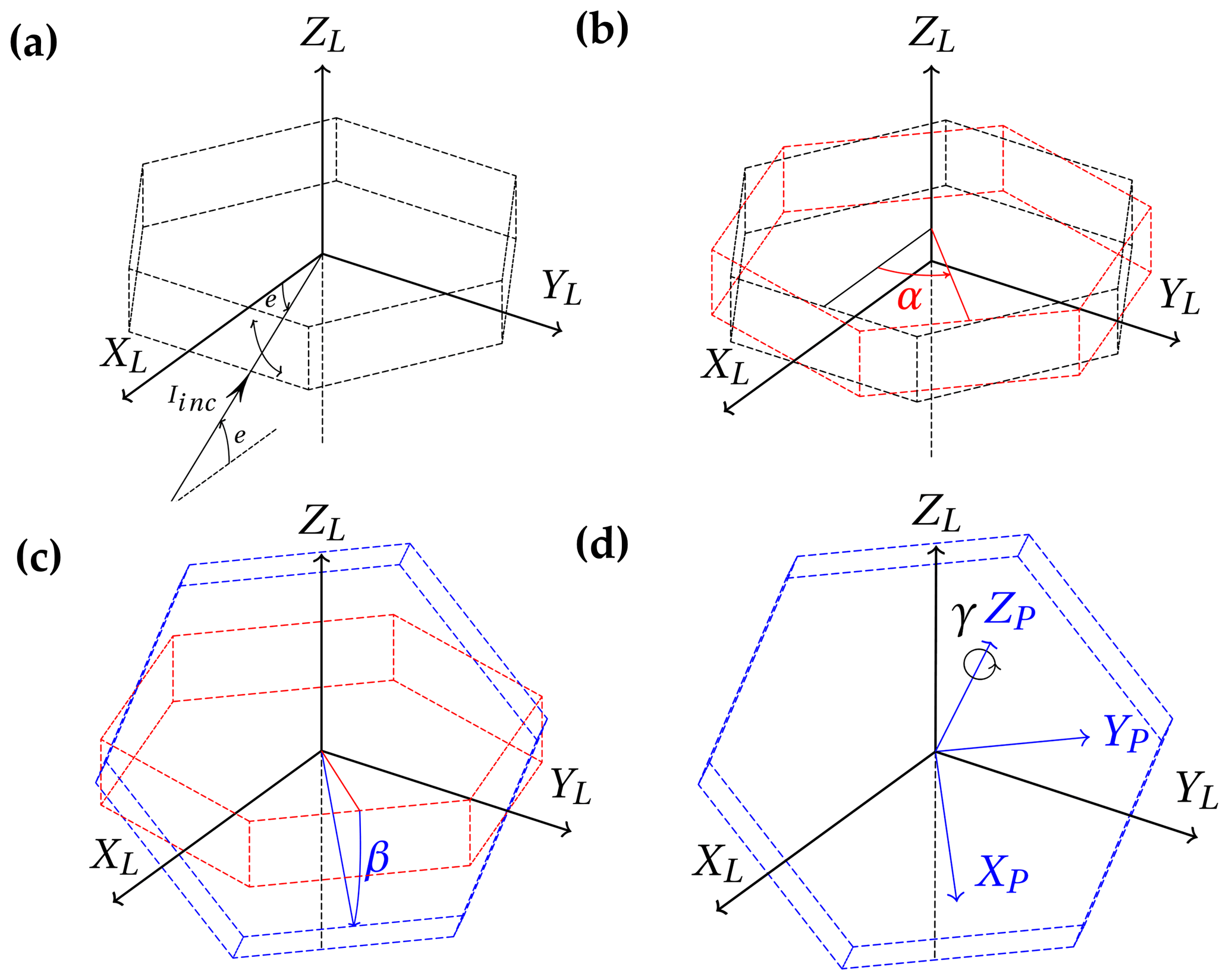
Figure 3 Illustration of the orientation preference of a particle specified with Euler angles (α, β, γ) in which a hexagonal plate is used as an example. Panel (a) shows the laboratory coordinate system OX_LY_LZ_L and the particle with reference orientation ($\mathit{\alpha }=\mathit{\beta }=\mathit{\gamma }=\mathrm{0}$). The incident beam comes from the elevation angle of e. Panels (b), (c), and (d) depict how angles α, β, and γ uniquely determine the orientation of a particle, respectively. The particle coordinate system OX_PY_PZ_P is shown in panel (d) with solid blue lines.

3.3 Raw single-scattering properties: level A

To improve the accuracy of raindrop shape representation in the forward radar operator ZJU-AERO, it is essential to apply an established raindrop model that accounts for various effects such as the surface tension, hydrostatic and aerodynamic pressures, and static electric forces. By incorporating these factors, a more accurate geometric representation of observed raindrop shapes can be achieved compared to the most commonly used spheroid model, as proved by photographs of water drops falling at the terminal velocity in air (Pruppacher et al., 1998). In a study conducted by Chuang and Beard (1990), an equilibrium differential equation was utilized to iteratively determine the shape of a falling raindrop with a given mass which corresponds to a specific diameter D_eq. The obtained results were then fitted to Chebyshev polynomials as follows (Chuang and Beard, 1990):

$$\begin{array}{}\text{(19)}& \mathit{\chi }\left(\mathit{\theta }\right)={\displaystyle \frac{D_{\mathrm{eq}}}{\mathrm{2}}}\left[\mathrm{1}+\sum _{i=\mathrm{0}}^{\mathrm{10}}{a}_n\left(D_{\mathrm{eq}}\right)\left(\mathrm{1}+\cos \left(n\mathit{\theta }\right)\right)\right].\end{array}$$

This equation involves the distance between the raindrop's surface to its mass center, denoted as χ(θ), where θ is the zenith angle in spherical coordinates (see Fig. 4d). Chuang and Beard (1990) provided Chebyshev coefficients a_n(D_eq) on diameter grids. Therefore, for a given D_eq size, the corresponding Chebyshev coefficients can be obtained through interpolation.

The Chebyshev model of raindrops deviates from xy-plane reflectance symmetry, resulting in a flatter bottom surface compared to the spheroid. Conversely, the top surface of the raindrop described by the Chebyshev model is sharper. Note that the disparity between the two models becomes more pronounced with increasing D_eq, as shown in Fig. 4a–c. It can be noted from Fig. 4c that larger raindrops are more prone to aerodynamic effects and therefore have a flatter base compared to the reference “spheroid”.

Comparing the optical properties of two shapes with significantly different aspect ratios cannot reveal the effects resulting from introducing Chebyshev shapes. To address this, we defined the aspect ratio of the Chebyshev model in Fig. 4d, which represents the vertical maximum dimension b^′ versus the horizontal maximum dimension a^′. Figure 5 illustrates a comparison between the aspect ratio of the Chebyshev model, as defined above, and the aspect ratio of the commonly used spheroid raindrop model (Thurai et al., 2007; Brandes et al., 2002). It is apparent that for common raindrops with D_eq<8 mm, the aspect ratios of the two models are approximately equal. Therefore, we can infer that the differences in optical properties between the spheroid and Chebyshev models arise from higher-order shape specifications rather than the first-order aspect ratio parameter (also proved by comparisons between two shapes with identical aspect ratio; figure not shown).

A detailed examination of the optical properties of Chebyshev model rain droplets and their sensitivity against traditional spheroid model were conducted by Ekelund et al. (2020). To compare the radar variables between the spheroid and Chebyshev models, they used an extended precision version of the EBCM T-matrix code (Mishchenko and Travis, 1994). However, it is important to note that the EBCM may encounter numerical instability issues due to the extremely high imaginary part of refractive indices for liquid water around the K band (10–40 GHz), where the Ku and Ka bands are located. To ensure integrity and accuracy, this study presents an optical property database (with a user-friendly radar operator interface) for the Chebyshev raindrop model at the Ku and Ka bands (13.6 and 35.5 GHz, respectively) using the IITM code (Bi et al., 2013).

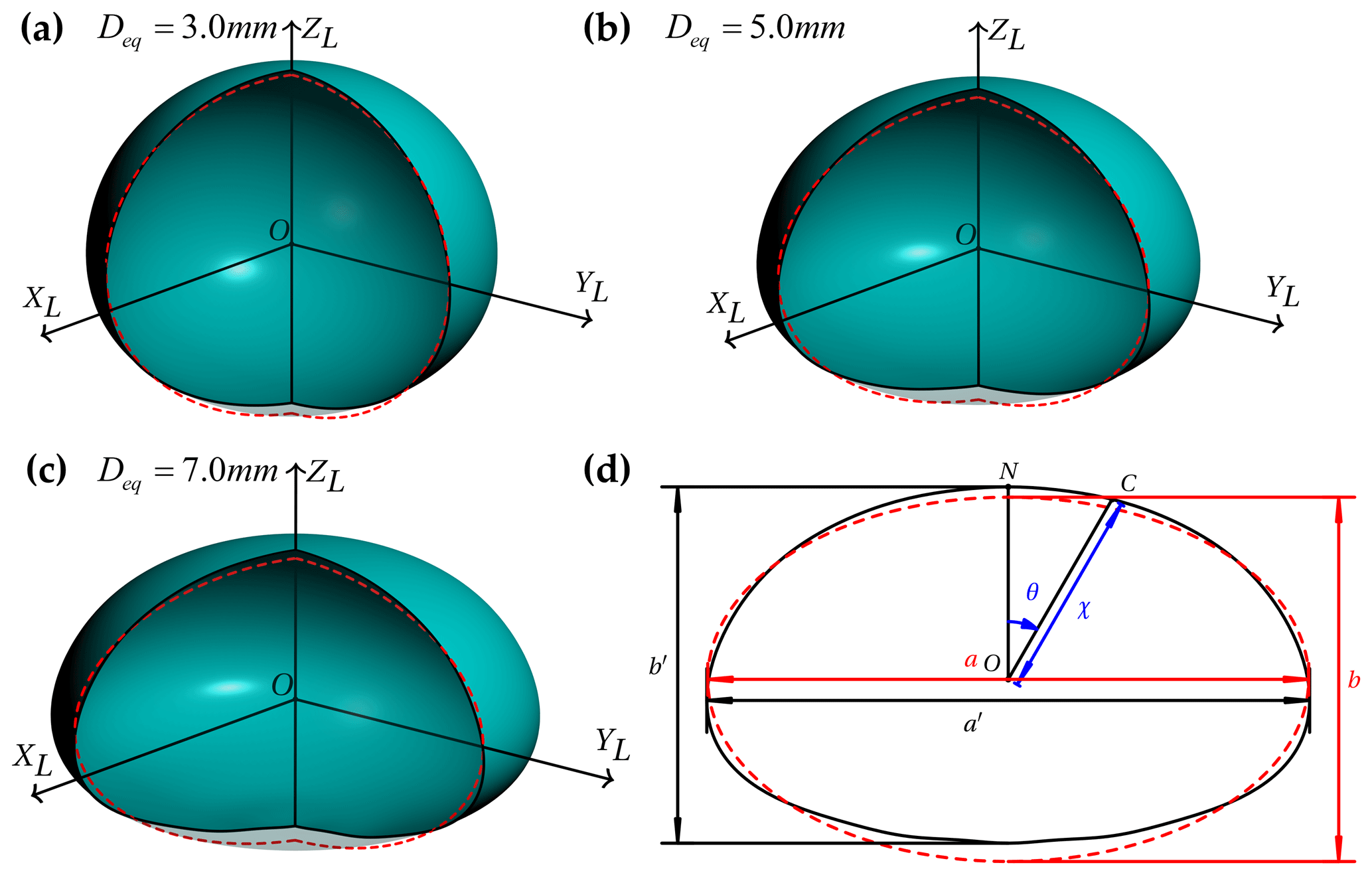
Figure 4 Illustration of raindrops described based on the Chebyshev model. Panels (a), (b), and (c) display the shapes of the Chebyshev raindrop with equal-volume-sphere diameters (D_eq) of 3, 5, and 7 mm, respectively. Panel (d) shows the vertical cross section of the Chebyshev shape corresponding to panel (c), and it also illustrates how the aspect ratio $b^{\prime }/a^{\prime }$ is defined for a Chebyshev raindrop. The dashed red lines in all panels show the spheroid model with identical D_eq values for comparison. The aspect ratio of the spheroid is defined as $b/a$, and b and a are shown in panel (d). The Chebyshev shapes in panels (a)–(c) were set to be partially transparent and displayed in an azimuth angle range [$-\mathit{\pi }/\mathrm{6}$, $\mathit{\pi }/\mathrm{2}$].

To better understand the impact of single-scattering properties on radar variables, it is necessary to analyze the RSSP–level A database. Additionally, we choose to introduce intermediate quantities called the “SSP factors for radar variables”, which are illustrative and facilitate our understanding of how SSPs of a given particle size affect radar variables.

The SSP factor “[z_h]” for the horizontal reflectivity “z_h” is defined as

$$\begin{array}{}\text{(20)}& \left[z_{\mathrm{h}}\right]={\displaystyle \frac{\left(Z_{\mathrm{11}}-Z_{\mathrm{12}}-Z_{\mathrm{21}}+Z_{\mathrm{22}}\right)\cdot \left(\mathrm{2}{\mathit{\lambda }}^{\mathrm{4}}\right)}{{\mathit{\pi }}^{\mathrm{4}}\mathrm{|}{K}_{\mathrm{w}}{\mathrm{|}}^{\mathrm{2}}}}.\end{array}$$

Here, the quantity enclosed in the square brackets [z_h] indicates the SSP factor of the radar variable z_h. We can perform a particle ensemble mean on it, which is often indicated by angle brackets, as follows (Zhang, 2016):

$$\begin{array}{}\text{(21)}& 〈\left[z_{\mathrm{h}}\right]〉={\displaystyle \frac{\mathrm{2}{\mathit{\lambda }}^{\mathrm{4}}}{{\mathit{\pi }}^{\mathrm{4}}\mathrm{|}{K}_{\mathrm{w}}{\mathrm{|}}^{\mathrm{2}}}}\left(〈Z_{\mathrm{11}}〉-〈Z_{\mathrm{12}}〉-〈Z_{\mathrm{21}}〉+〈Z_{\mathrm{22}}〉\right)=z_{\mathrm{h}}.\end{array}$$

Here, the last equals sign is the definition of the horizontal reflectivity (see Eq. D1 in Appendix D).

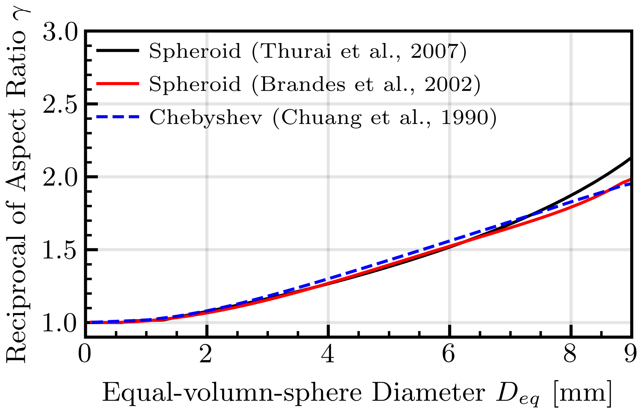
Figure 5 The aspect ratio–diameter relationships as reported in the literature. The vertical axis is the reciprocal of the aspect ratio (i.e., γ). Thurai et al. (2007) and Brandes et al. (2002) fitted in situ measurements of two-dimensional video disdrometer (2DVD) measurements by segmented polynomials to give the explicit γ–D_eq expressions, while the aspect ratios of the Chebyshev raindrop are estimated with the Chebyshev coefficients recorded by Chuang and Beard (1990) with the method mentioned in Fig. 4d. Since raindrops with their D_eq size larger than 8 mm are beyond the typical size range (Zhang, 2016) and rarely found in nature (Kobayashi and Adachi, 2001), the relationships given by Brandes et al. (2002) and Chuang and Beard (1990) end at 9 mm.

Similarly, the SSP factor “[a_h]” for the horizontal attenuation coefficient “a_h” is defined as follows (the extinction cross section by essence):

$$\begin{array}{}\text{(22)}& \left[a_{\mathrm{h}}\right]=K_{\mathrm{11}}-K_{\mathrm{12}}={\mathit{\sigma }}_{\mathrm{ext},\mathrm{h}}.\end{array}$$

If we perform particle ensemble mean on it, then we find that it is proportional to the definition of the horizontal attenuation coefficient (see Eq. D5 in Appendix D):

$$\begin{array}{}\text{(23)}& 〈\left[a_{\mathrm{h}}\right]〉=\left(〈K_{\mathrm{11}}〉-〈K_{\mathrm{12}}〉\right)={\mathrm{10}}^{\mathrm{3}}\cdot a_{\mathrm{h}}.\end{array}$$

As shown by Eqs. (21) and (23), these factors ([z_h] and [a_h]) are the equivalent radar parameters of radar reflectivity z_h and specific attenuation a_h, respectively, for a single particle of size D_eq. For further SSP factors for a level A database diagnoses, please refer to Fig. 8.

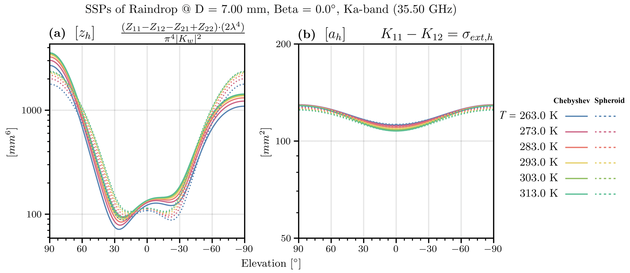
Figure 6 (a) SSP factor of horizontal reflectivity and (b) SSP factor of horizontal attenuation against the elevation angle of a radar beam for a raindrop with an equal-volume-sphere diameter of 7.0 mm at the Ka band (35.5 GHz), together with their expression in the upper-right corner of the panels. The SSP factors of the level A database are displayed for different temperatures with lines in different colors. The results of the Chebyshev raindrop analysis are indicated with solid lines, while those of spheroid raindrop are indicated with dotted lines. The database entries for β=0° are shown. Negative elevation angles indicate that the beams are pointing (slanting) downwards. The variations with respect to temperature entirely originate from temperature dependence of water dielectric constants.

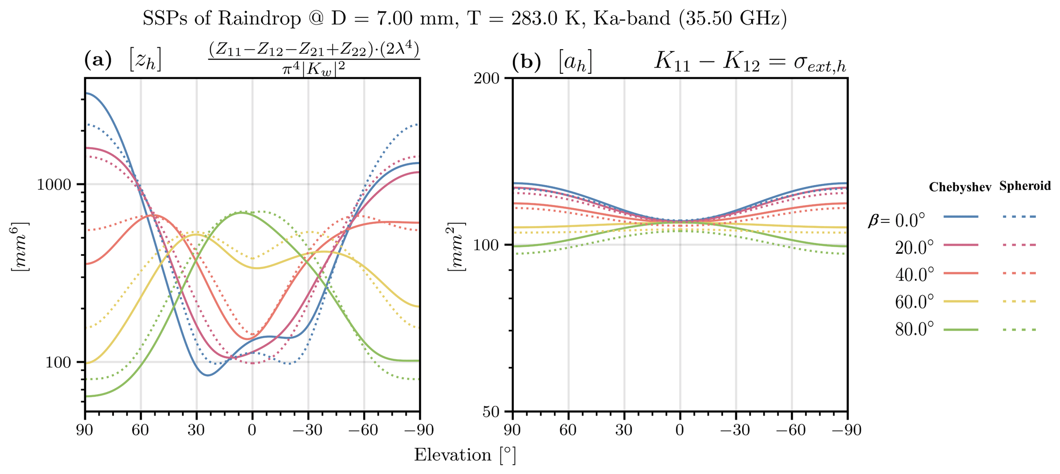
Figure 7 The results for different orientation angles (β) are displayed with different colors in a manner resembling Fig. 8. The database entries for temperature = 10 °C (283 K) are shown.

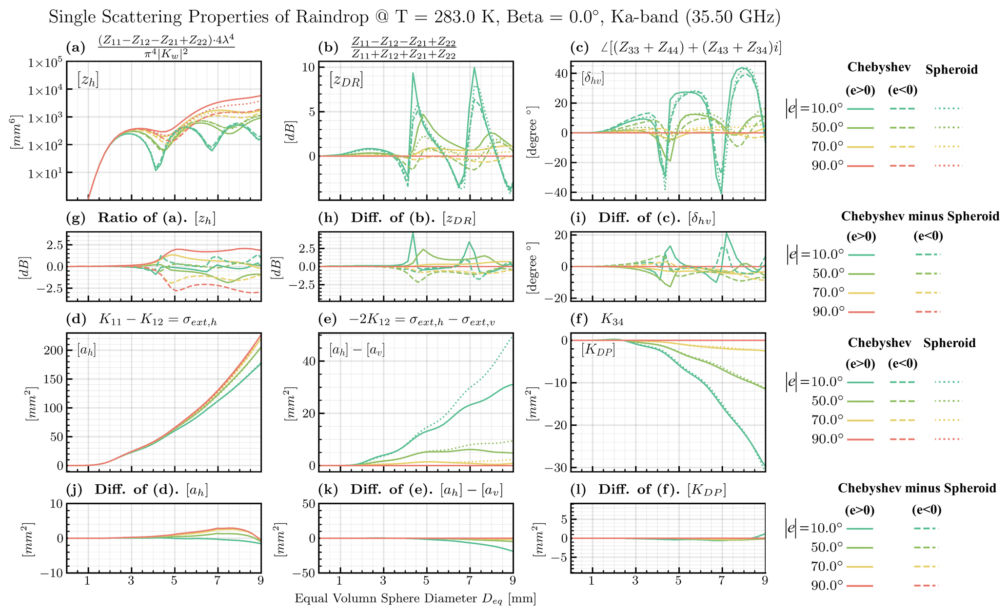
Figure 8 The SSP factors of intrinsic radar variables (indicated in the upper-left corner) for the Chebyshev model and the spheroid raindrop models against the equal-volume-diameter of the liquid particles at the Ka band (35.5 GHz) and 283 K. Lines with different colors display the SSP factors for different elevation angles of the radar beam. Results of positive elevation angles for spheroids are indicated by solid lines, while those of negative elevation angles are indicated by dashed lines. Since the results of spheroids have xy-plane reflectance symmetry, the negative and positive results are merged as dotted lines. The flatter auxiliary plots in panels (g)–(l) (the second and fourth rows) below the major plots (a)–(f) (the first and third rows) display the corresponding differences (or ratios) of optical properties between the Chebyshev model and the spheroid models, respectively. The first column shows horizontal polarization SSP factors ([z_h] and [a_h]) mentioned in Figs. 6 and 7, the second column shows SSP factors contributing to observed differential reflectivity ([z_DR] and [a_h]–[a_V]), and the third column shows the SSP factors contributing to the observed total phase shift ([δ_hv] and [K_DP]).

It is not surprising to observe that the scattering properties exhibited symmetry with respect to the radar beam elevation angle, e=0°, for the spheroid model. This is because spheroids possess reflectance symmetry in the xy plane. However, this symmetry does not hold true for the Chebyshev model. We find that the SSP factor [z_h] has a more pronounced peak than spheroids near the nadir (specifically, e=90°, which is frequently encountered for the vertical-profiling cloud radar), as shown in Fig. 6a. Conversely, the peak near the zenith (i.e., $e=-\mathrm{90}\mathit{°}$ for the spaceborne radar) is weaker. This phenomenon is also found for the Chebyshev model at 94.1 GHz (Ekelund et al., 2020), which can be attributed to its flatter bottom surface and sharper top surface geometries in Ekelund et al. (2020), as depicted in Fig. 4. Additionally, we find that the [z_h] factor for ground-based scattering geometries (e=0–20°) is close to the values obtained for the spheroid model. However, deviations from the spheroid model were typically much smaller for lower-frequency bands, such as the Ku band (13.6 GHz) (figure not shown here).

However, the forward scattering properties such as [a_h] of the Chebyshev model still maintain their symmetry with respect to the beam elevation angle e=0°, which can be easily understood based on the reciprocal theory (Van de Hulst, 1981). It is important to note that the attenuation effects of Chebyshev raindrops are slightly stronger compared to spheroid ones for near-nadir and zenith-scattering geometries.

Figure 6 also demonstrates the stability of the deviations between the Chebyshev model and the spheroid model (CmS hereafter) in terms of the temperature dimension. However, the finding is different for [z_h] against the orientation preference dimension β (see Fig. 7a). It can be interpreted that a varying orientation presents a significantly different “view” of raindrops to the observer, while the varying temperature essentially keeps the same view of the raindrop with different dielectric constants. It was found that the positive and negative CmSs of [z_h] at nadir and zenith, respectively, hold true only if β<20°. In cases where particle groups have larger canting angles (β>20°), the CmS for [z_h] can produce a reversal of their signs (Fig. 7a). Since the column “orientation preference” in Table 1 shows that the standard deviation of β=7° for raindrops under normal turbulence conditions does not exceed this threshold for raindrops, we can infer that the CmS deviations found for β=0° only show a minor decrease if orientation averaging is performed.

As for [a_h], we learned that the conclusions of CmS at β=0° always hold true when β is sufficiently large (Fig. 7b).

We also examined the results across the entire PSD range of raindrops shown in Fig. 8. It was found that the aforementioned CmS results for [z_h] were significant when D_eq>3 mm (Fig. 8g), while those for [a_h] were significant only for larger raindrops (i.e., D_eq>5 mm; see Fig. 8j).

It is worth mentioning that raindrops had significantly higher [z_h] for larger absolute values of the beam elevation angle e (Fig. 8a). This can be easily understood since the zenith or nadir observation geometries tend to capture a larger cross section of oblate-spheroid-like models.

As for other SSP factors of polarimetric radar variables, the CmS deviations are either not stable against size spectra (Fig. 8h and i) or too small in terms of its base magnitude (Fig. 8l), making them not significant for a particle group. However, the CmS effects of SSP factor for differential attenuation ([a_h] − [a_v]) in Fig. 8k is significant at low absolute elevation angles, indicating that the SSP factor of the vertical polarization attenuation [a_v] is significantly stronger for the Chebyshev model (considering [a_h] is close for two shapes at low absolute elevation angles in Fig. 8j).

The canting angle of raindrops is generally small, so the CmS deviations of SSP factors found in Figs. 6 and 8 only show a minor decrease in the level B ASSP database when compared to the curves of β=0° in the level A RSSP database. Hence, we omit any further analysis of the orientation averaging of raindrops and SSP factors of the level B database here.

3.4 PSD options and analysis of level B to level C LUT conversion

In this subsection, we will focus on describing the PSD options for raindrops and the methods used to analyze their impacts on the conversion of SSP factors of radar variables to intrinsic radar variables (i.e., the ASSP to BSP conversion).

In ZJU-AERO, a total of six options for PSD schemes for raindrops were available, all of which are listed in Table 3. All schemes were designed for rain modeled by a single-moment microphysics scheme with exponential distribution assumptions. Each PSD schemes can be visualized as a N₀–Λ curve, as shown in Fig. 9.

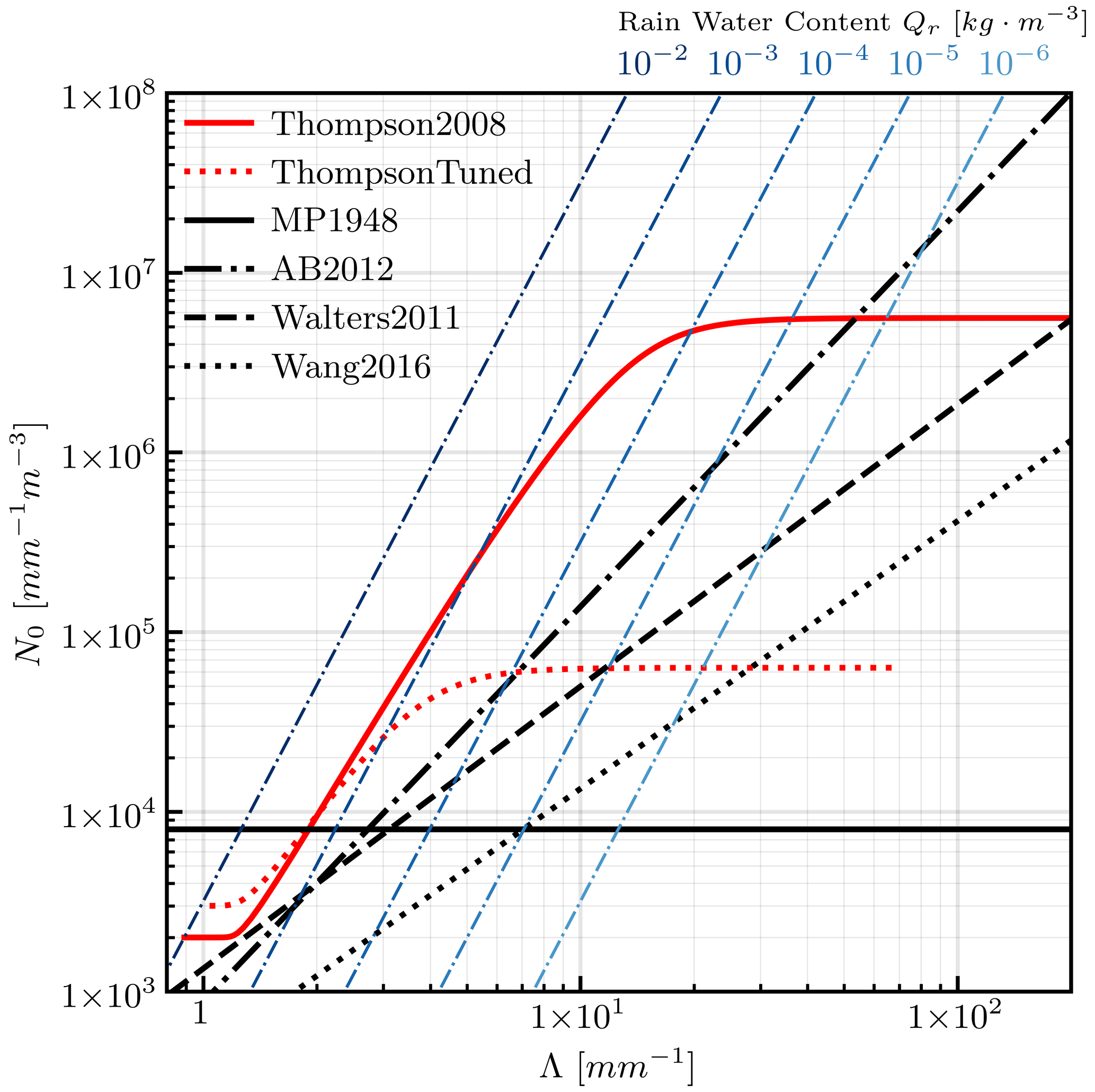
Figure 9 The N₀–Λ diagram introduced by Abel and Boutle (2012). All the PSD schemes mentioned in Table 1 are represented as either black or grey curves in this figure. The blue dashed–dotted lines represent isolines of water concentration for rain Q_R. The curves extend to the upper-right corner as Q_R increases. The solution of (N₀, Λ) for a given PSD scheme and Q_R can be found by determining the intersection of colored curves and black/gray curves in this diagram.

The constant N₀ parameterization originally proposed by Marshall and Palmer (1948) and used in microphysics packages, such as Hong and Lim (2006), provides a rough approximation for various liquid precipitation scenarios. However, modern PSD schemes for rain, such as the one by Thompson et al. (2008), aim to capture the observed transition from high concentrations of drizzle-sized drops (D_eq<0.5 mm) in stratocumulus clouds to PSDs dominated by large millimeter-sized raindrops in heavy precipitation.

We classified the six PSD schemes into two groups by how the intercept parameter N₀ is determined. Group A is characterized by a power law N₀–Λ relationship, which is represented as a straight line in the dual-log-scale diagram in Fig. 9. On the other hand, the intercept parameter, N₀, for group B schemes follows a formalization described by Eq. (24), transitioning from N₂ to N₁ as the water mass concentration, Q_R, increases. This can be visualized as the tanh-like curves shown in Fig. 9:

$$\begin{array}{}\text{(24)}& N_{\mathrm{0}}=\left({\displaystyle \frac{N_{\mathrm{1}}-N_{\mathrm{2}}}{\mathrm{2}}}\right)\tanh \left[{\displaystyle \frac{\left(Q_{R\mathrm{0}}-Q_R\right)}{\mathrm{4}{Q}_{R\mathrm{0}}}}\right]+\left({\displaystyle \frac{N_{\mathrm{1}}+N_{\mathrm{2}}}{\mathrm{2}}}\right).\end{array}$$

The values of the reference rainwater mass concentration Q_R0 and the dynamic range [N₂, N₁] of the intercept parameter are displayed in the group B in Table 3.

Table 3 The parameters of rain particle size distribution (PSD) schemes available in ZJU-AERO. Group A of the PSD schemes, namely (1) MP1948, (2) AB2012, (3) Walters2011, and (4) Wang2016, can be generalized as a power law N₀–Λ relationship (see Eq. 9), as stated in Sect. 2.3, while group B of the PSD schemes, namely (1) Thompson2008 and (2) ThompsonTuned, can be generalized as Eq. (24), in which N₀ is simply determined by the mass concentration of rain. The last scheme, tagged as ThompsonTuned, was proposed in the present study to fit of the observations in the case study presented in Sect. 4. Note that the 10-based or 1000-based coefficients in the “x₁” column of group A are used for unit conversion as the parameters are taken from various studies with divergent unit conventions. Also note that the parameter Q_R0 is originally a mixing ratio (in units of kg kg⁻¹) rather than mass concentration (in units of kg m⁻³), but we have performed the conversion by assuming ρ_air=1.225 kg m⁻³ of standard atmosphere at sea level (1013.25 hPa). It should be noted that the constant air density is only used here to qualitatively determine the position of the Thompson2008 and ThompsonTuned N₀–Λ curves in Fig. 11. Diagnostic air density is used in the actual PSD solver of ZJU-AERO.

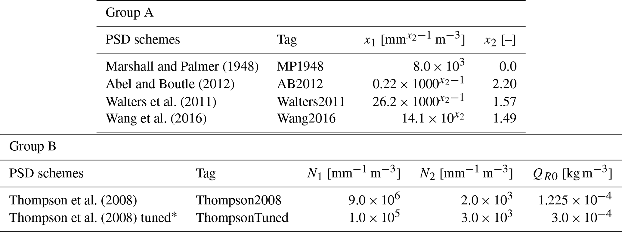
^* The ThompsonTuned PSD scheme is for numerical tests only; therefore, it is not a user option in Table 1.

Figure 9 demonstrates the large variability in the intercept parameter N₀ for a specified rainwater content (RWC) among different PSD schemes. That variability can be shown by measuring the vertical coordinate difference in the intersection points between a given iso-RWC line and different N₀–Λ lines of PSD schemes. For PSD schemes expressed by an exponential distribution, a larger intercept parameter N₀ means more smaller drops when the RWC is fixed. Therefore, the Thompson scheme (Thompson et al., 2008) prioritizes smaller drops, while the Wang scheme (Wang et al., 2016) places more emphasis on larger drops.

According to global aircraft in situ measurements carried out by Abel and Boutle (2012), the six single-moment (SM) microphysics assumptions in Table 3 cover the natural variability in the raindrop PSDs ranging from continental precipitation to maritime precipitation. Typical continental PSD with intensive large drops, such as in Wang et al. (2016), and typical maritime PSD, such as in Thompson et al. (2008), with a large population of drizzle-sized raindrops are both present. That is why we have chosen the six SM microphysics schemes for the PSD sensitivity test.

It should be noted that although SM microphysics has been used for years and will continue to be used, it has obvious shortcomings with respect to reproducing the polarimetric features observed in convective and stratiform events. Since double-moment (DM) microphysics in CMA-MESO is still experimental, the consistent DM scheme in ZJU-AERO is still in the development stage. However, the natural variability in the raindrop PSDs for DM microphysics schemes is still within what is displayed in Fig. 9; therefore, it is safe to use those SM assumptions for a sensitivity test.

To explore the effects of different PSD schemes on the radar variables, a new intermediate quantity called “backscatagrand” is analyzed in Fig. 10, which is a spectra of particle size defined as the product of the horizontal backscattering cross section σ_bsca,h(D) and size distribution function N(D). It helps us identify particles for which the size range dominates the energy of the backscattering.

The idea of analyzing backscatagrand was inspired by the definition of “extagrand” used in the analysis of the RTTOV-SCATT bulk-scattering tables (Geer et al., 2021), which helps with diagnosing the single-particle contribution to the extinction coefficients in the radiative transfer simulations of passive microwave sounders. The concept of extagrand is based on the insight that the total extinction of an ensemble of particles is primarily influenced by a fraction of particles within a narrow diameter range. Therefore, by analyzing the SSP for particles within that size range, we can infer the BSP of the entire ensemble of particles. The extagrand σ_ext(D)N(D) (in units of mm m⁻³) is factorized as the product of the mass distributions m(D)N(D) (in units of kg mm⁻¹ m⁻³) and the extinction cross section per unit volume ${\mathit{\sigma }}_{\mathrm{ext}}\left(D\right)/m\left(D\right)$ (in units of mm² kg⁻¹). These quantities are determined by PSDs and SSPs, respectively. The extagrand quantities are appreciable only for size ranges in which both the mass distribution m(D)N(D) and mass extinction efficiency ${\mathit{\sigma }}_{\mathrm{ext}}\left(D\right)/m\left(D\right)$ are large enough to produce significant products of extagrand.

However, for weather radar applications, the principal quantity is backscattering rather than the extinction, as is the case for passive instruments. Hence, we try to analyze quantities of the horizontal polarization backscattering cross section per volume ${\mathit{\sigma }}_{\mathrm{bsca},\mathrm{h}}\left(D\right)/m\left(D\right)$ (parallel definition of mass extinction efficiency, which we refer to as mass backscattering efficiency hereafter) and the backscatagrand σ_bsca,h(D)N(D) (parallel definition of extagrand) in which σ_bsca,h(D) indicates the horizontal polarization backscattering cross section.

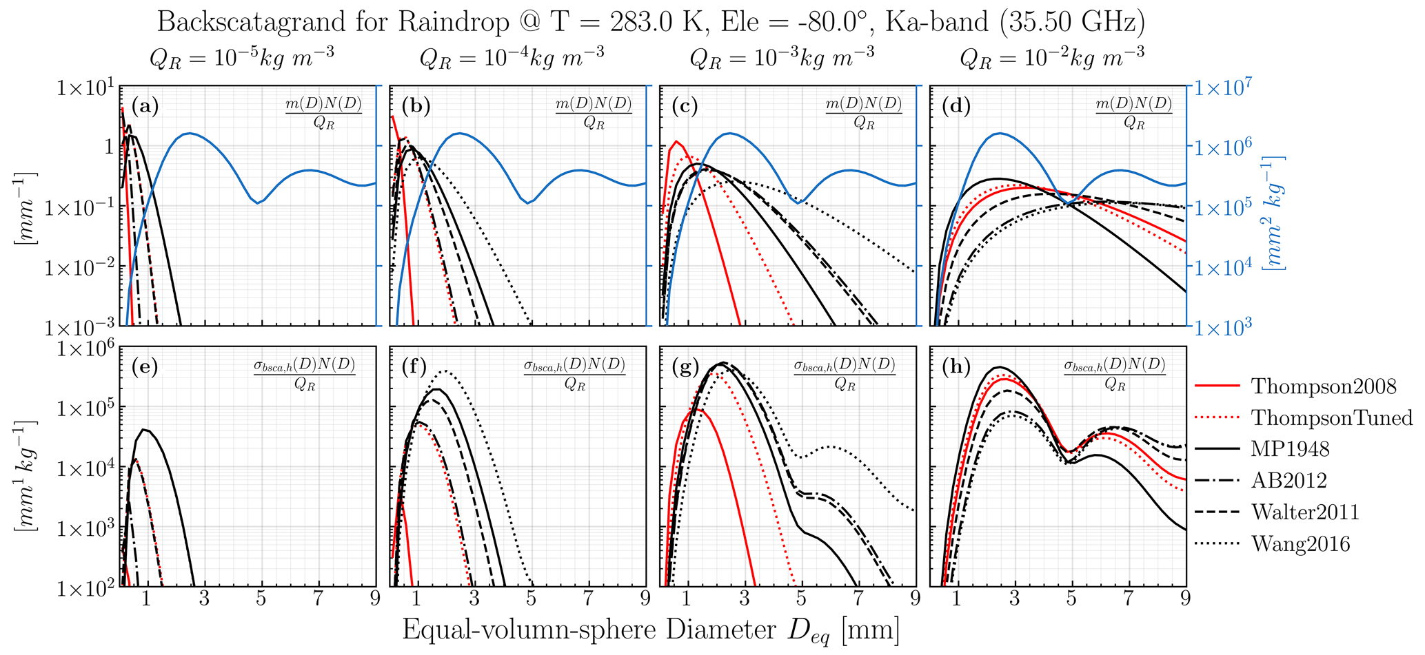
Figure 10 The analysis of the integration of single-particle horizontal polarization backscattering over the PSD. The horizontal polarization backscattering cross section σ_bsca,h was obtained using the applied single-scattering properties (ASSP) in level B of the Chebyshev raindrop database. The regular conditions of spaceborne radar (T=283 K; $e=-\mathrm{80}\mathit{°}$) at the Ka band (35.5 GHz) (indicated in the title) were considered. The first row displays the mass distribution m(D)N(D) (normalized by rain mass concentration Q_R) for five PSD schemes and four water concentration settings, while the mass backscattering efficiency ${\mathit{\sigma }}_{\mathrm{bsca},\mathrm{hv}}\left(D\right)/m\left(D\right)$ is indicated by the blue lines with the blue axis, and labels are marked on the right. The second row shows the quantity of backscatagrand σ_bsca,hv(D)N(D) (also normalized by the rain mass concentration Q_R) for different PSD schemes and water concentrations, which is a measure that particles contribute to the horizontal reflectivity z_h (the principal intrinsic radar variable). The red or black curves in the first row multiplied by the blue curve exactly yield the second row's curves.

In Fig. 10, we can find that the mass distributions and backscattering contribution spectrum (i.e., the so-called backscatagrand) exhibit large uncertainties due to the natural variability in the PSD schemes. The mass backscattering efficiency has multiple oscillations caused by the resonance effect, particularly in high-frequency bands such as the Ka band. Specifically, two important peaks of mass backscattering efficiency at D_eq=2.5 mm and D_eq=6.5 mm and one important dip at D_eq=5.0 mm exist (solid blue line in Fig. 10d). For extremely heavy precipitation ($Q_R\sim {\mathrm{10}}^{-\mathrm{2}}$ kg m⁻³), the peak of the mass distributions might coincide with the dip of the mass backscattering efficiency at D_eq=5.0 mm. This phenomenon is unique to PSD schemes that contain more large drops (such as Wang2016 and AB2012), which leads to a loss of the bulk reflectivity if the total mass of the raindrop remains constant.

Under all but extremely heavy-precipitation conditions (Q_R<10⁻² kg m⁻³; see Fig. 10c and g), the Thompson2008 PSD scheme stands out as an outlier. Its extremely large N₀ compared to other schemes (see Fig. 9) leads to a significantly smaller peak in mass distributions as small as D_eq<1.0 mm, while the peak of other PSD schemes is approaching the first peak of the mass backscattering efficiency at D_eq=2.5 mm. Accordingly, the total reflectivity computed with the Thompson2008 scheme must be much smaller at $Q_R={\mathrm{10}}^{-\mathrm{3}}$ kg m⁻³ than those computed with other PSDs.

The relative importance of particles in the entire spectrum can be diagnosed with the curves of backscatagrand, which is the ultimate goal to introduce this concept. For example, we can learn from Fig. 10h that the contribution of backscattering is dominated by particles with the diameter D_eq at around 2.5 mm for the MP1948 scheme, while the contribution from particles of 2.5 mm size and 6.5 mm size are almost equally important for the Wang2016 and AB2012 schemes. To go further, we can infer that the CmS deviations mentioned in Sect. 3.3 can only affect the bulk-scattering properties computed with the Wang2016 and AB2012 schemes, since the CmS deviations of backscattering are only significant for particles with D_eq>3 mm (Fig. 8g).

3.5 Bulk-scattering properties: level C

Figure 11 shows the intrinsic radar variables for the Chebyshev model which were computed using the BSP database and the spheroid model at the Ka band. In Sect. 3.4, we hypothesized based on the backscatagrand plot, and we can now confirm these hypotheses individually.

1. The application of PSD schemes, such as Wang2016, can result in a significant reduction in the reflectivity Z_H (by approximately 5 dBZ) for extremely heavy-precipitation scenarios compared to the default PSD scheme MP1948 (refer to Fig. 11a; $Q_R\sim {\mathrm{10}}^{-\mathrm{2}}$ kg m⁻³).

2. The reflectivity Z_H computed by the Thompson2008 scheme for moderately heavy-precipitation scenarios is considerably lower (by over 10 dBZ) compared to other PSD schemes in group A in Table 1 (refer to Fig. 11a' $Q_R\sim {\mathrm{10}}^{-\mathrm{3}}$ kg m⁻³).

3. The CmS deviations are only significant (reducing Z_H by about 2 dBZ) for extremely heavy-precipitation scenarios and PSD schemes that emphasize larger drops, such as Wang2016 (refer to Fig. 11a, $Q_R\sim {\mathrm{10}}^{-\mathrm{2}}$ kg m⁻³).

4. The CmS deviations of attenuations, α_H, are never significant for regular mass concentrations of rain Q_R (see Fig. 11b). This finding can be explained by the fact that the CmS deviations in RSSP (Fig. 8j) are significant only if D_eq>7 mm, which represents a group of drops sharing a small fraction of the mass distribution, even for extremely heavy precipitation.

From Fig. 11, it can be concluded that the horizontal polarization intrinsic radar variables Z_H and α_H at the Ka band (actually also for the Ku band; not shown here) are more sensitive to the uncertainty in the PSD schemes than the CmS optical property deviations for spaceborne radar observation geometries. The CmS deviations are only notable for extremely heavy-precipitation scenarios in which large drops are prominent. Those conclusions focusing on the Ka band (35.6 GHz) generally agree well with what was found by Ekelund et al. (2020).

The sensitivities of intrinsic polarimetric radar variables with respect to CmS deviations for ground-based radar bands (S, C, or X band) and viewing geometries were found to be negligible. Therefore, they are not shown here.

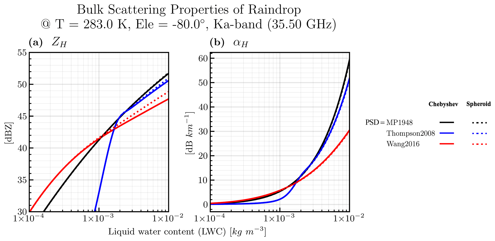
Figure 11 The intrinsic radar variables against the liquid water content (mass concentration of rain Q_R) computed with the bulk-scattering property (BSP) level C database of the Chebyshev raindrop and spheroid models, which are indicated by solid and dotted curves, respectively. A typical condition of the spaceborne radar (T=283 K; $e=-\mathrm{80}\mathit{°}$) at the Ka band (35.5 GHz) was considered. Panels (a) and (b) display the two intrinsic radar variables (horizontal reflectivity Z_H and horizontal attenuation α_H) that can be diagnosed from the corresponding factors of SSP in Fig. 8a and d, respectively. The colors of the curves are used to indicate three typical PSD schemes chosen from Table 1. Here, only the results of PSD schemes MP1948, Thompson2008, and Wang2016 are displayed because MP1948 is a benchmark traditional PSD scheme, while Thompson2008 and Wang2016 are representative of typical maritime and continental precipitation PSDs, respectively.

4 Case studies

To assess the simulation capabilities of ZJU-AERO, we conducted case studies using real-world data and investigated the sensitivities of the PSD schemes and the new Chebyshev raindrop model. For this study, we chose the GPM core satellite (referred to as GPM hereafter) and specifically analyzed the overpass of Typhoon Haishen, the first super-typhoon of the 2020 northwest Pacific typhoon season, on 5 September 2020 at 09:21 UTC. We used the simulation and observation data from the dual-frequency precipitation radar (DPR) aboard the GPM for our analysis.

To conduct the ZJU-AERO simulations, we utilized model grid data generated by the operational run of CMA-MESO, which was initialized at 00:00 UTC on 5 September 2020. The CMA-MESO grid data had a horizontal resolution of 3 km and consisted of 50 vertical layers. Note that the WSM6 microphysics package was selected for the CMA-MESO operational run. However, any forced PSD schemes could be applied in the simulation of the radar operator, as mentioned in Sect. 2.3.

To demonstrate the reliability of the forward radar operator for ground-based polarimetric radars, we have also performed a case study of a mesoscale convective system (MCS) which can be found in the user manual (see the “Code and data availability” section). The results are reasonable but relatively trivial compared to previous radar operators, so we will not display them in this section.

4.1 Simulation of a tropical cyclone case

According to Iguchi (2020), the GPM/DPR's Ku-band radar basically follows the instrument characteristics of the Tropical Rainfall Measuring Mission (TRMM) Precipitation Radar (PR), while the new Ka-band radar is sensitive to light rain and snow. By combining data from two channels, more accurate estimates of DSD parameters can be obtained (Rose and Chandrasekar, 2006; Liao et al., 2014). The Ka-band radar has two modes (Iguchi et al., 2010), namely (1) a high-sensitivity mode for light rain and snow (high-sensitivity beam) and (2) a matched-beam mode in which the sampling volumes of the Ka- and Ku-band radar are collocated (matched beam). However, since 21 May 2018, the GPM/DPR has switched its scan pattern so that now a full swath can be considered the matched beam in the evaluation of a forward radar operator. Therefore, in this case study, we used data from the Ka band in the matched-beam mode to estimate DSD and drop morphology parameters.

The dual-frequency ratio (DFR) is defined as the difference between the log-space-measured reflectivity at two channels (Ku and Ka bands). Previous studies have shown that the DFR can be used to distinguish between stratiform and convective rain (Le and Chandrasekar, 2012).

Figure 12 displays the observation and simulation of the Ku-band radar reflectivity at different levels, with the last row showing the mismatch between them (i.e., the OmB of reflectivity). Figure 13 presents the cross section of radar reflectivity between points A and B in Fig. 12 separately for the Ku and Ka bands. Additionally, the last column shows the DFR as defined above. The radar operator applied the ThompsonTuned PSD option (for developers only) and the Chebyshev morphology options A2 (see Table 3) for the category rain in the simulations. For snow, we use default option A2. For graupel, we use default option A2 and B1. The reflectivities in Fig. 12a–d are masked by a flag called “flagPrecip” (available at the ground) offered in the L2A swath data of GPM/DPR, while the simulation of reflectivity in Fig. 12e–h is masked by the sensitivity threshold of 12 dBZ to keep it the same with sensitivity of GPM/DPR observation. We applied the attenuation in simulations while using the “zFactorMeasured” product of GPM/DPR (no attenuation correction applied). As for the calculation of OmB reflectivity, the radar gates for which the reflectivity is undetectable (below the instrument sensitivity) either in the simulation or observation are filled with a “background” reflectivity of 0 dBZ to generate the OmB reflectivity.

Based on the comparison between observations and simulations in Figs. 12 and 13, it can be found that the regional model of CMA-MESO is able to capture some of storm structures, such as the cyclone eye and eyewall. However, the structures of outer spiral rain bands in the simulation (Figs. 12e and 13d) appear more contiguous and vague compared to the isolated towering bands depicted by the GPM/DPR measurements (Figs. 12a and 13a). Although the NWP model could not accurately predict the cloud and precipitation timing and position, the probability distribution of the simulated radar reflectivity should be unbiased when compared with observations (detailed examinations on that will be conducted in Sect. 4.2); otherwise, a systematic bias in the NWP model or the radar operator might be identified. Since (a) the precipitation forecast of CMA-MESO model can be frequently calibrated against a rain gauge network (Bárdossy and Das, 2008; Cattoën et al., 2020), and (b) a forecast lead time of 9 h is beyond the 6 h spin-up time of the rainwater content in CMA-NWP (Ma et al., 2021), we assume that the NWP model CMA-MESO has no significant bias in this case.

Notably, the freezing level in this case was found within the altitudes ranging from 4 to 5 km (see the 0 °C NWP model background isothermal line in Fig. 13), which is believed to contain abundant melting particles. Actually, the GPM/DPR observations revealed a weak bright-band (BB) signature below the freezing level, which can be recognized at the Ku band (with an average reflectivity enhancement of approximately 3 dB; see Fig. 13a) but is not so clear at Ka band (see Fig. 13b). As reported by long-term radar observation statistics of melting layers documented in Fabry and Zawadzki (1995), the magnitude of the BB signature in the melting layer is significantly weaker in deep-convection regions. Therefore, the weak BB signatures in the melting layer of this tropical cyclone case can probably be attributed to the large riming rates (Zawadzki et al., 2005) in the convective precipitation of tropical cyclone eyewall and rain bands. However, the simulations we conducted did not show a BB signature, which was attributed to not considering melting or mixed-phased particles and the shortcoming of the microphysics scheme. Considering the lack of melting schemes in ZJU-AERO, it is expected that the melting layer would exhibit a positive OmB signature due to lack of melting hydrometeors in ZJU-AERO. However, in Fig. 13g and h, we encountered difficulties in identifying a continuous positive mean bias of the OmB for both the Ku and Ka bands in the melting layer. This challenge arose due to the large mislocation errors in the precipitation predicted by the NWP model used in this study. To address this issue, future analysis could employ horizontal averaging or examine the probability distribution function of reflectivities in the melting layer. Implementation of melting particle models and their relevant validations will be a subject for upcoming publications.

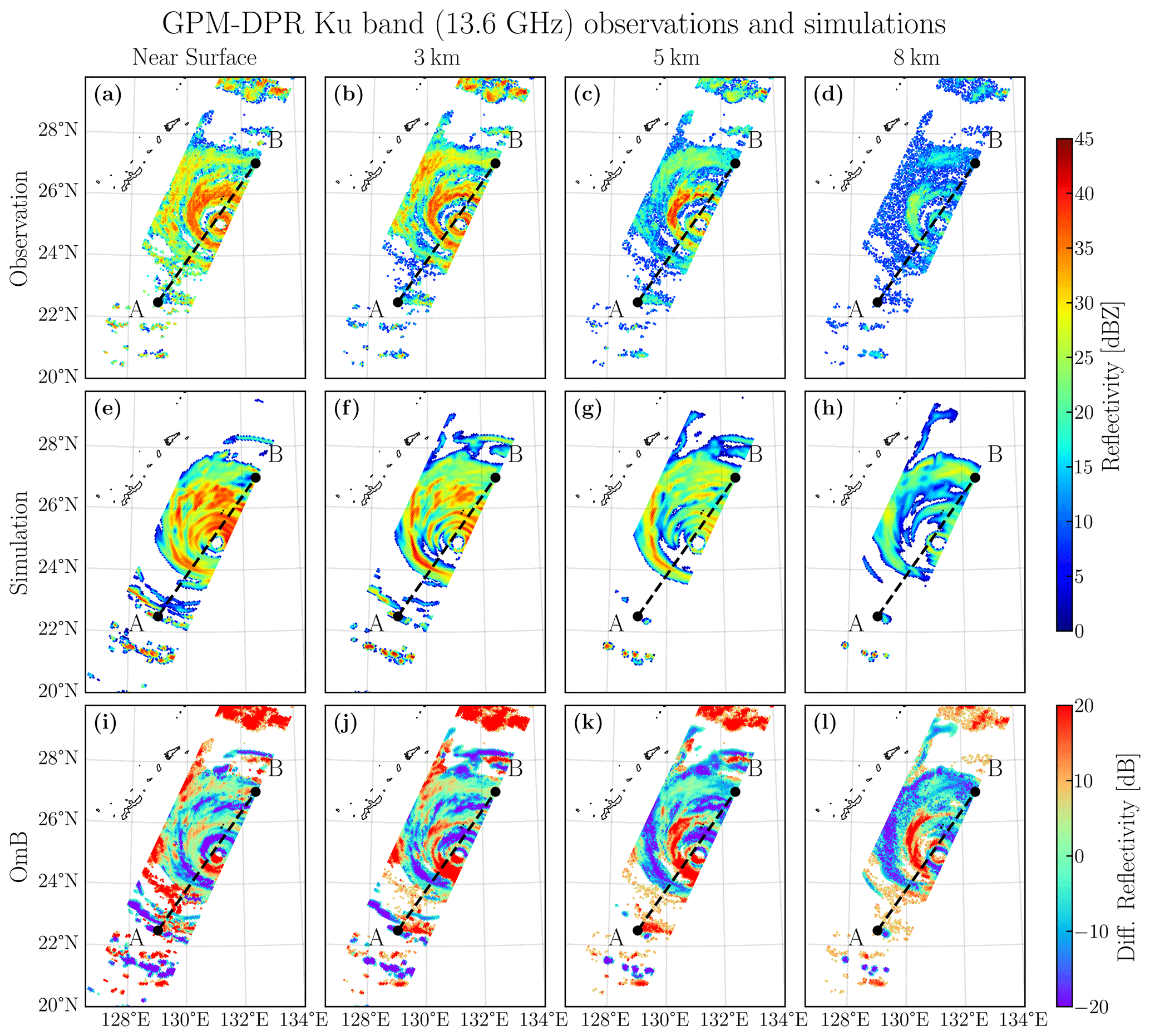
Figure 12 Panels (a)–(d) display the Global Precipitation Mission–Dual-frequency Precipitation Radar (GPM/DPR) observed radar reflectivity at the Ku band (13.6 GHz) for the overpass of Typhoon Haishen at 09:21 UTC on 5 September 2020. The results shown at different columns correspond to four altitude levels (i.e., near-surface (the first clutter-free gate) and 3, 5, and 8 km). The second row (panels e–h) shows the simulated radar reflectivity by applying the +9 h forecast output of the CMA-MESO (initiated at 00:00 UTC on 5 September 2020) to the ZJU-AERO. The last row (panels i–l) shows the observation minus simulation (OmB) of radar reflectivity of the four levels. The cross section indicated by the dashed line between A (22.5° N, 129° E) and B (27° N, 132.5° E) was selected for further studies, as shown in Fig. 13.

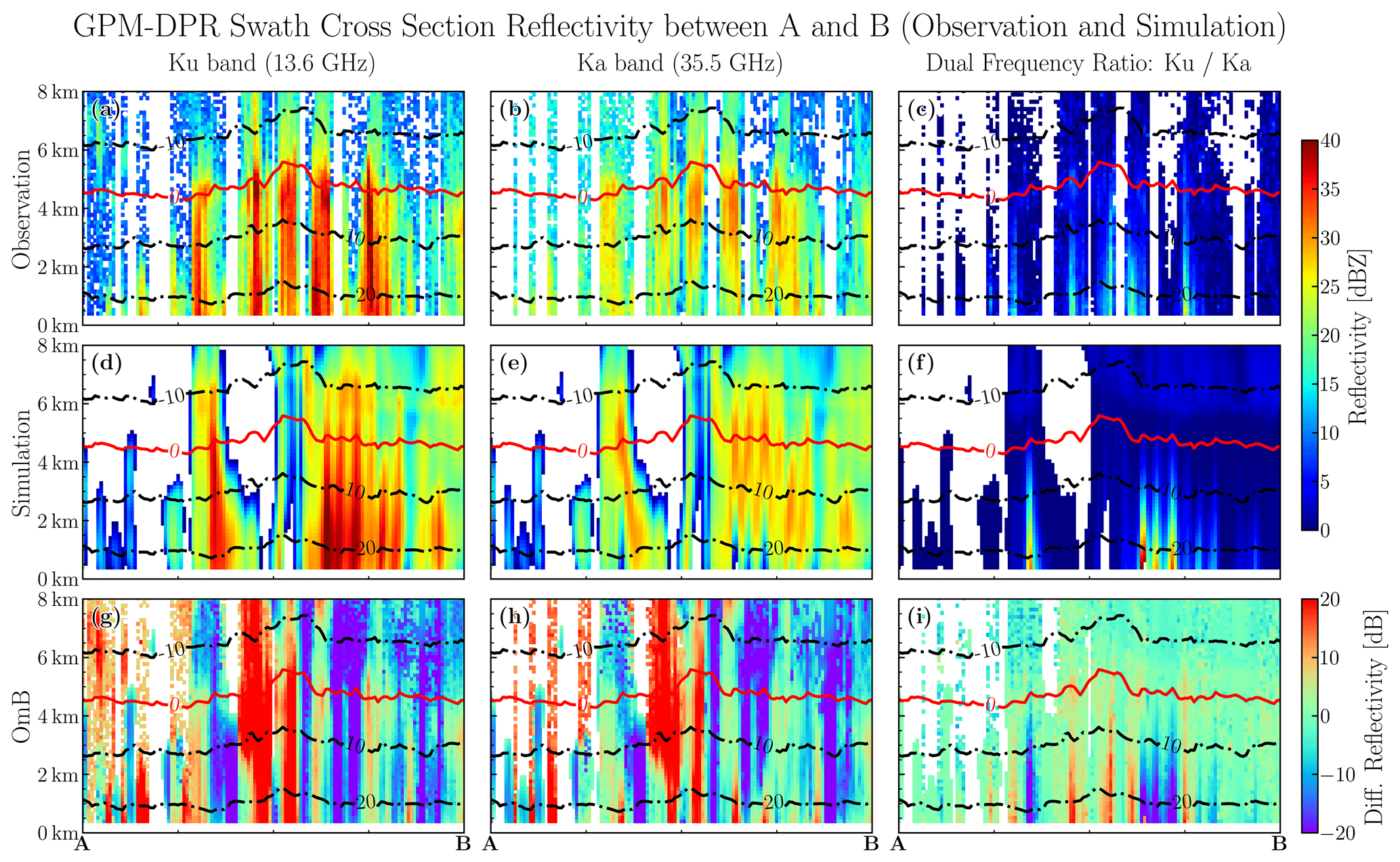
Figure 13 The cross section of the radar reflectivity indicated by the line AB in Fig. 12. The GPM/DPR observations are shown in the first row (panels a–c), simulations of the radar operator are shown in the second row (panels d–f), while the OmB of reflectivity is shown in the third row (panels g–i). As for the arrangement of panels in the column view, the first, second, and third columns display the results of the Ka and Ku bands and the dual-frequency ratio (DFR; $\mathrm{Ku}/\mathrm{Ka}$), respectively. The temperature of the model background state is indicated by isothermal lines in each panel. Numbers of the contour labels have the unit of degrees Celsius.

Moreover, extremely large DFR values (>30 dB) were found in simulations (Fig. 13f) but not in observations (Fig. 13c) in the 0 to 2 km layer, which could be attributed to an over-estimation of the attenuation in the Ka-band simulation for heavy precipitation (Fig. 13e). This hypothesis is supported by two facts: (1) many weak reflectivity (∼ 10 dBZ) regions are found right beneath the strong reflectivity gates aloft at around 4 km for the Ka band (Fig. 13e), and (2) the weak reflectivity regions of the Ka band collocate with the strong reflectivity region (∼ 40 dBZ) of the Ku band (Fig. 13d).

The OmB plots, as shown in Figs. 12 and 13, are useful tools for verifying and calibrating new observation operators and identifying their deficiencies. Overall, the results are generally reasonable and demonstrate the capability of ZJU-AERO to simulate the reflectivity of dual-frequency spaceborne radar such as GPM/DPR. More analysis on the bias of the probability distribution of reflectivities/DFR will be presented in the next subsection.

4.2 Sensitivity assessments on hydrometeor PSDs and morphologies

We also performed sensitivity assessments for the PSD and non-spherical morphology options of the rain hydrometeor category. Figure 14 shows the observation and simulation distributions of radar reflectivity at the Ku and Ka bands and the dual-frequency ratio (DFR) at two altitude layers (0–2 and 2–4 km). Since we were tuning the liquid hydrometeor, the melting and solid layers in the last two columns (4–6 and 6–8 km) did not concern us. The radar operator applied the Chebyshev morphology in all simulations except the group with the label “ThompsonTuned(Spheroid)”, which was simulated with the spheroid raindrop option. Other options of ZJU-AERO are identical with those in Fig. 12.

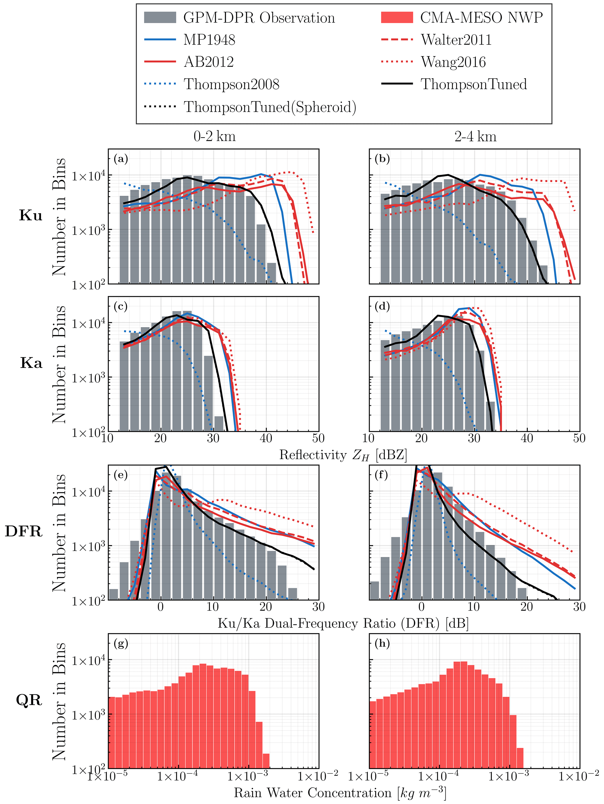
Figure 14 The observation and simulation distributions of radar reflectivity at the Ka band (the first row), Ku band (the second row), and the dual-frequency ratio (DFR) (the third row). The last row shows the log-scale histogram of rainwater content (Q_R) predicted by CMA-MESO. The data of the distributions were gathered from the reflectivity of all the radar gates in the four altitude layers (i.e., the 0–2 km layer and 2–4 km layer, as the tags on the top of the columns suggest). The first two layers (0–2 and 2–4 km) were primarily composed of liquid hydrometeors, while the layers above 4 km contain melting and solid particles (results not shown here). The observation distributions of reflectivity are shown by grey bars in the panels, while the simulation distributions are indicated by curves with different colors and styles. The data of observations and simulations are binned equivalently between 12 and 50 dBZ with a bin size of 2 dB.

Based on statistical analysis (see Fig. 14g and h), we found that the mass concentration of rain in the CMA-MESO at the storm rain bands was primarily dominated by moderately heavy rain ($Q_R\sim {\mathrm{10}}^{-\mathrm{3}}$ kg m⁻³) rather than extremely heavy rain ($Q_R\sim {\mathrm{10}}^{-\mathrm{2}}$ kg m⁻³). According to Sect. 3.5 and Fig. 11, applying the Thompson2008 PSD leads to a significant reduction in the simulated reflectivity in conditions of moderately heavy rain ($Q_R\sim {\mathrm{10}}^{-\mathrm{3}}$ kg m⁻³), which is consistent with our findings in Fig. 14a, b, c, and d for the Ku and Ka bands of liquid layers.

Due to the strong wind shear in the rain bands of the tropical cyclone, large drops can be broken apart (Radhakrishna, 2022), causing the rain PSD in such conditions to behave irregularly and deviate from the prevailing parameterizations. Figure 14a, b, c, and d demonstrate that almost all the PSD schemes significantly overestimated the reflectivity for both Ku and Ka bands, except for the Thompson2008 scheme, which underestimated the reflectivity.

To address the discrepancy, we designed a new PSD scheme, referred to as ThompsonTuned, by tuning the parameters in Eq. (24). The optimization procedure can be formulated as follows.

1. We use a scoring method to quantify the match between observation and simulation histograms, as proposed by Geer and Baordo (2014):

   $$\begin{array}{}\text{(25)}& s=\sum _{j=\mathrm{1}}^{\mathrm{nbands}}\sum _{i=\mathrm{1}}^{\mathrm{nbins}}\left|\log \left({\displaystyle \frac{N_{\mathrm{sim}}^j\left(i\right)}{N_{\mathrm{obs}}^j\left(i\right)}}\right)\right|.\end{array}$$

   Here, s represents the final score, with N_sim and N_obs indicating the counts in the ith bins of the simulation and observation histograms, respectively. The superscript “j” denotes jth band. To prevent infinite values in the summation, we assume a count of 0.1 in bins with empty values in either the simulation or observation histograms.

2. Next, we establish a grid of free parameters for optimization which includes three parameters (N₁, N₂, and Q_R0). Due to the broad range of these free parameters, the grid is set up in a quasi-logarithmic scale.

3. Subsequently, simulations are conducted, and the score from Eq. (25) is evaluated for each grid point. By identifying an optimal region in the parameter space with the best score, we refine the grid in that region to pinpoint a more precise parameter subregion. This iterative process is carried out to fine-tune the parameters.

4. Finally, we identified an optimal point at which the black lines in Fig. 14a, b, c, and d closely matched the observed distributions. The parameters are listed in Table 3 and plotted in the N₀–Λ diagram in Fig. 9. The tuned PSD scheme is reasonable as it falls between the MP1948 and Thompson2008 schemes in the N₀–Λ diagram, with an emphasis on smaller particles compared to MP1948. This may be attributed to the unusual DSD in tropical cyclones.

While no in situ DSD observations are available to support the tuned PSD schemes used in this study, the implications of the tuning experiments are interesting, considering that the matched-beam observation of the Ku and Ka bands were designed for the DSD estimation.

As suggested by Sect. 3, the CmS effects were negligible in this case, as it is difficult to discriminate the solid and dashed black lines in Fig. 14. This is likely due to the moderately heavy rainfall in tropical cyclones with strong wind shears which prevent the large drops from highlighting the CmS deviations. However, the CmS effects could be significant in cases of extremely heavy rain in the supercell storms, according to our observation system simulation experiment (OSSE). An OSSE of GPM/DPR overpassing a mesoscale convective system (recorded with extreme heavy-precipitation events) reported CmS decrease effects of more than 1 dB at the Ku band and more than 2 dB at the Ka band (figures not shown). This sensitivity test is consistent with what we found in Fig. 11a and demonstrates the value of introducing the Chebyshev-shaped raindrop model in certain scenarios (e.g., vertical pointing cloud radar, airborne radar, and spaceborne radar working at high-frequency bands). As for polarimetric radar variables such as Z_DR and K_DP for ground-based radar at side-viewing geometry, the CmS effects are generally negligible.

5 Summary and ongoing tasks

In summary, Sect. 2 of our study introduced the basic formulations and concepts of the design in the ZJU-AERO. These concepts included the general procedure of the software, radar-variable calculations, and the available hydrometeor settings (shape parameters, dielectric constant models, canting angles, and particle size distributions). Formulations of polarimetric radar variables are derived starting from single-particle back-scattering Mueller matrix Z and extinction matrix K.

In Sect. 3, we highlighted the unique features of ZJU-AERO, specifically its multi-layered design for the optical database of non-spherical particles. We demonstrated this by displaying the scattering properties using the example of the Chebyshev-shaped raindrop particle model and comparing it to the properties of traditional spheroid raindrops. We conducted LUT demonstrations for two database layers, namely level A (raw single-scattering properties database) and level C (bulk-scattering property database). We also introduced a new intermediate quantity named backscatagrand to diagnose the PSD integrations of optical properties. We concluded that the Chebyshev-shaped raindrop model shows noticeable differences in the bulk-scattering properties (compared to spheroid model) only at zenith- and nadir-viewing geometries and for millimeter-wavelength radar bands. This difference is more prominent for continental DSD models (e.g., Wang2016) with larger drops. These deviations can reach up to 2–3 dB at the Ka band for spaceborne radars in heavy continental precipitation regions where large drops dominate. Given the lower uncertainties in simulating the reflectivity of the liquid phase compared to the solid and melting phases, such a difference deserves attention in specific applications such as comparing data from ground-based and spaceborne radar observations (Warren et al., 2018).

Furthermore, in Sect. 4, we validated the simulation reliability and capability of ZJU-AERO by analyzing a case study of a tropical cyclone using input from the CMA-MESO for simulating spaceborne radar observations. We found that ZJU-AERO provides reasonable simulation results, except for the bright-band signature at the melting layer, which can be attributed to the current version of ZJU-AERO and does not consider melting or mixed-phased particles. We also performed sensitivity assessments of PSDs and morphology options for rain in ZJU-AERO and found that the ThompsonTuned single-moment PSD scheme provides the best fit of the reflectivity histogram in the simulation to the GPM/DPR observation. However, using either the Chebyshev-shaped raindrop particle model or the spheroid model makes little difference to the simulation results since the tropical cyclone precipitation has a maritime DSD where small drops dominate.

Currently, ZJU-AERO is an efficient forward radar operator that has the advantage of handling the complexities of non-spheroid particle models. Therefore, it is a powerful research tool for studying the sensitivities of polarimetric radar observations with respect to the non-sphericity of hydrometeor particles. It also applies parallel acceleration techniques to boost its performance, allowing operational applications of data assimilation in NWP models employing single-moment (SM) microphysics (such as CMA-GFS/MESO). A ZJU-AERO forward radar operator can be applied in data assimilation (DA) studies using indirect DA methods such as the Bayesian approach (Caumont et al., 2010) and direct DA methods such as ensemble Kalman filter (EnKF) that both require no tangent linear (TL) or adjoint (AD) versions of the forward radar operator.

ZJU-AERO also has some limitations. For example, it currently cannot be applied in DA research based on the variational method. Simplification and linearization works are involved to obtain a TL/AD version of the forward operator. Moreover, PSD solvers for DM microphysics schemes have already been implemented in ZJU-AERO for the experimental CMA-MESO DM microphysics, but there are many validation and evaluation works to be done. Also, unlike the EMVORADO, which use a distributed-memory parallel design and interface with the COSMO-NWP model online, ZJU-AERO applies a shared-memory parallel design, and the NWP model input should be stored in external files.

Overall, the results were satisfactory, and the ZJU-AERO operator is ready for experimental and operational usage. However, several aspects of ZJU-AERO still need improvement, and we have listed the ongoing development tasks as follows:

1. Improve frozen hydrometeor modeling by introducing irregular-shaped aggregates and riming snow.

2. Improve the modeling of melting particles (including melting snow, melting graupel, and melting hail) using layered inhomogeneous modeling rather than an effective medium approximation for the mixture matrix.

3. Compute the optical properties of melting particles using the IITM code and extend the SSP/BSP database with a new dimension of the water fraction.

4. Develop more concrete models for single-crystal, aggregated, and rimed snow to replace the “soft spheroid” model and create a corresponding SSP/BSP database.

5. Model hail as non-spheroid and inhomogeneous particles.

6. Include cloud ice, which plays an significant role in the high-frequency bands of spaceborne radar.

7. Do more tests for double-moment microphysics schemes in CMA-MESO.

8. Conduct more case studies, particularly with measurements from the spaceborne radar FY-3 RM/PMR. Notably, the L1 product of spaceborne radar FY-3 RM/PMR has been accessible online (released by the National Satellite Meteorological Center (NSMC) on 22 November 2023). We have already implemented an external I/O (input/output) module to interface with the data format of FY-3 RM/PMR in ZJU-AERO, but the time coverage of observation data is too limited for us to find a good demonstration case. Therefore, more case studies and fine-tuning should be conducted with future measurements from FY3RM-PMR.

In conclusion, ZJU-AERO is an observation operator that facilitates the exploitation of measurement data from both spaceborne and ground-based radars. Its versatility and effectiveness make it a valuable tool for data assimilation in CMA-GFS/MESO. Moreover, ZJU-AERO has the potential to be applied in various other studies within a wide range of contexts.

Appendix A: Specifications on spaceborne radar trajectory solver

For spaceborne radars aboard rain measurement satellite platforms, such as the Tropical Rainfall Measuring Mission/Global Precipitation Measurement/FengYun-3 Rain Measurement (TRMM/GPM/FY-3 RM), the trajectory of the radar beam can be treated without considering the beam-bending effects while still maintaining precision. The WGS84 coordinates of satellites, denoted as A (scLat, scLon, scAlt), in addition to the center of the footprint, A₁ (lat, lon), can be obtained through the satellite radar L1/L2 products (hereafter referred to as swath files). These coordinates can then be used to calculate the local elevation angle of a given radar gate, C, using the knowledge of trigonometry in Fig. A1b. The length of segments H and R_E can be computed by converting the (latitude, longitude, and altitude) WGS84 coordinates to the Earth-centered, Earth-fixed (ECEF) coordinates. The range of radar gate AC is provided by the spaceborne radar observation system in the L1 product of GPM/DPR known as “scRangeEllipsoid” (Iguchi et al., 2010). When neglecting the beam-bending phenomenon in the spaceborne radar detection, the local elevation angle, e^′, can be expressed as $e^{\prime }=e-\mathit{\alpha }$ in which e is the elevation angle on the satellite. The angle α could be determined using trigonometry, given that AC represents the range of the radar gate C.

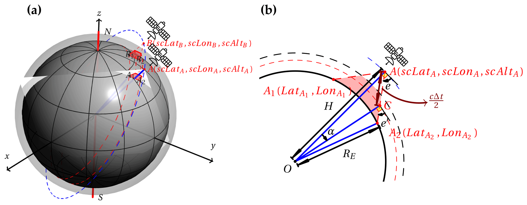
Figure A1 Conceptual graphs depicting the observation geometry of spaceborne radar, with panel (a) showing a 3D graph illustrating the inclined orbit of a precipitation-measuring satellite by a dashed blue line. The satellite positions A and B were selected from the orbit, and the triples (scLat, scLon, scAlt) on A and B were measured using the WGS84 coordinate system. The spaceborne radar is capable of performing cross-track scans, creating a swath between two parallel red cycles on the Earth. The space spanned by two red isosceles trapezoids indicates that the valid scan volume is in the troposphere between orbit positions A and B in the troposphere. In panel (a), we selected the white plane protruding from the Earth (a plane determined by the Earth's center “O” in addition to the two end footprints (A₁ and A₂) of a single cross-track scan) to examine the geometric relationships in panel (b).

Appendix B: Appendix B: grids of LUT dimensions in ZJU-AERO

The grids of LUT dimensions are presented in Table B1. Only the Z and K matrix elements that appear in the formulas of polarimetric radar variables in Eqs. (D1)–(D8) are stored in the database. For temperatures, we set the minimum temperature for super-cooled liquid particles as 233 K, considering that homogeneous freezing starts at lower temperatures. For solid hydrometeors, the lowest temperature in the database is 203 K, and lower environment temperatures encountered are taken as 203 K. We provided LUTs for six bands that are widely used for ground-based and spaceborne weather radars. The ranges of diameters and aspect ratios for solid hydrometeors are suggested by observations of field research (Garrett et al., 2015), while the range of diameters and aspect ratios of the liquid hydrometeor have already been discussed in Sect. 3.3. The number of diameter bins is sufficient to produce a reasonable size spectrum of hydrometeors for various hydrometeor mass concentrations, as shown in Fig. 10. The range of mass concentration grids for BSP LUTs is the same as that of Geer et al. (2021). Other external LUTs, such as Eriksson et al. (2018), need to undergo format conversions and interpolations (e.g., for different diameter grids) before it can be applied in ZJU-AERO.

Table B1 Grid specifications for the lookup table (LUT) dimensions in ZJU-AERO. The format “[START:A, END:B, STEP:C]” represents a sequence of numbers ranging from A to B with an increment of C. The format “LIN[MIN:A, MAX:B, NUMBER:C]” denotes a sequence of evenly spaced numbers on a linear scale ranging from A to B with a total number of C values, while “LOG[MIN:A, MAX:B, NUMBER:C]” denotes a sequence of evenly spaced numbers on a log scale.

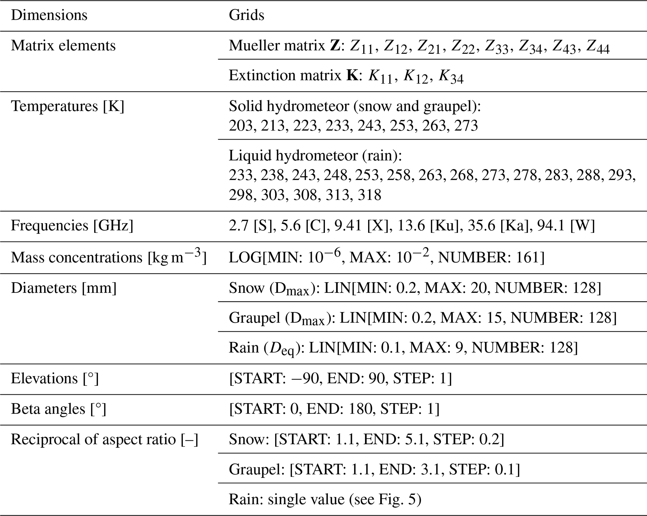
To alleviate the truncation and quadrature error in the particle size integration, a renormalization technique is applied after the particle number in each size bin is calculated. We first calculate the renormalization factor κ as follows:

$$\begin{array}{}\text{(B1)}& \mathit{\kappa }={\displaystyle \frac{\sum _{i=\mathrm{1}}^{\mathrm{nbins}}m\left(D_i\right)N\left(D_i\right)\mathrm{\Delta }D}{Q_{\mathrm{m}}}}.\end{array}$$

Here, m(D_i) is the mass of hydrometeor particle with a diameter of D_i, and N(D_i) is the particle number in that size bin, while ΔD is the diameter step of the numerical integration. Then (κ<1) gives the ratio between the mass concentration presented by our PSD and the mass concentration of hydrometeors given by NWP model Q_m. Then we can calculate the corrected particle number distribution N^corr(D_i):

$$\begin{array}{}\text{(B2)}& N^{\mathrm{corr}}\left(D_i\right)={\displaystyle \frac{N\left(D_i\right)}{\mathit{\kappa }}}.\end{array}$$

Appendix C: Forward scattering alignment (FSA) and backward-scattering alignment (BSA)

Although the optical properties of hydrometeors are consistently computed and stored in the FSA convention, this convention is not used for mono-static radar applications. Figure C1 displays the differences between the back-scattering alignment (BSA) convention and the FSA convention (Chandrasekar, 2001). The incident light propagates along −X_L direction and comes into contact with the particle at the origin O. $\widehat{h}$, $\widehat{v}$, $\widehat{k}$ are used to represent unit vectors of horizontal polarization, vertical polarization, and the propagation direction of electromagnetic waves, respectively. If we use the definition of $\widehat{h}$ and $\widehat{v}$ unit vectors under the FSA convention, then the horizontal unit vector of backscattering light is inconsistent with the incident light (${\widehat{h}}_{\mathrm{FSA}}^{\mathrm{inc}}$, ${\widehat{v}}_{\mathrm{FSA}}^{\mathrm{inc}}$, ${\widehat{k}}_{\mathrm{FSA}}^{\mathrm{inc}}$) = ($-{\widehat{h}}_{\mathrm{FSA}}^{\mathrm{bsca}}$,${\widehat{v}}_{\mathrm{FSA}}^{\mathrm{bsca}}$, $-{\widehat{k}}_{\mathrm{FSA}}^{\mathrm{bsca}}$), where “bsca” indicates backscattering light. To resolve this convention conflict between the polarimetric radar observation system and scattering computation, BSA forces the following relationship by reversing the direction of the backscattering horizontal unit vector definition: ($-{\widehat{h}}_{\mathrm{FSA}}^{\mathrm{bsca}}$, ${\widehat{v}}_{\mathrm{FSA}}^{\mathrm{bsca}}$, $-{\widehat{k}}_{\mathrm{FSA}}^{\mathrm{bsca}}$) = (${\widehat{h}}_{\mathrm{BSA}}^{\mathrm{bsca}}$, ${\widehat{v}}_{\mathrm{BSA}}^{\mathrm{bsca}}$, ${\widehat{k}}_{\mathrm{BSA}}^{\mathrm{bsca}}$). Hence, the amplitude-scattering matrix in the BSA convention is related to that of FSA as follows:

$$\begin{array}{}\text{(C1)}& \begin{array}{rl}{\left[\begin{array}{ll}{S}_{\mathrm{hh}}& S_{\mathrm{hv}}\\ S_{\mathrm{vh}}& S_{\mathrm{vv}}\end{array}\right]}_{\mathrm{BSA}}& =\left[\begin{array}{cc}-\mathrm{1}& \mathrm{0}\\ \mathrm{0}& \mathrm{1}\end{array}\right]{\left[\begin{array}{ll}{S}_{\mathrm{hh}}& S_{\mathrm{hv}}\\ S_{\mathrm{vh}}& S_{\mathrm{vv}}\end{array}\right]}_{\mathrm{FSA}}\\ & ={\left[\begin{array}{ll}-S_{\mathrm{hh}}& -S_{\mathrm{hv}}\\ S_{\mathrm{vh}}& S_{\mathrm{vv}}\end{array}\right]}_{\mathrm{FSA}}.\end{array}\end{array}$$

The following amplitude-scattering elements used for polarimetric radar variable computation are represented in the BSA convention, unless otherwise stated (i.e., a conversion is needed in the core submodule before obtaining radar variables).

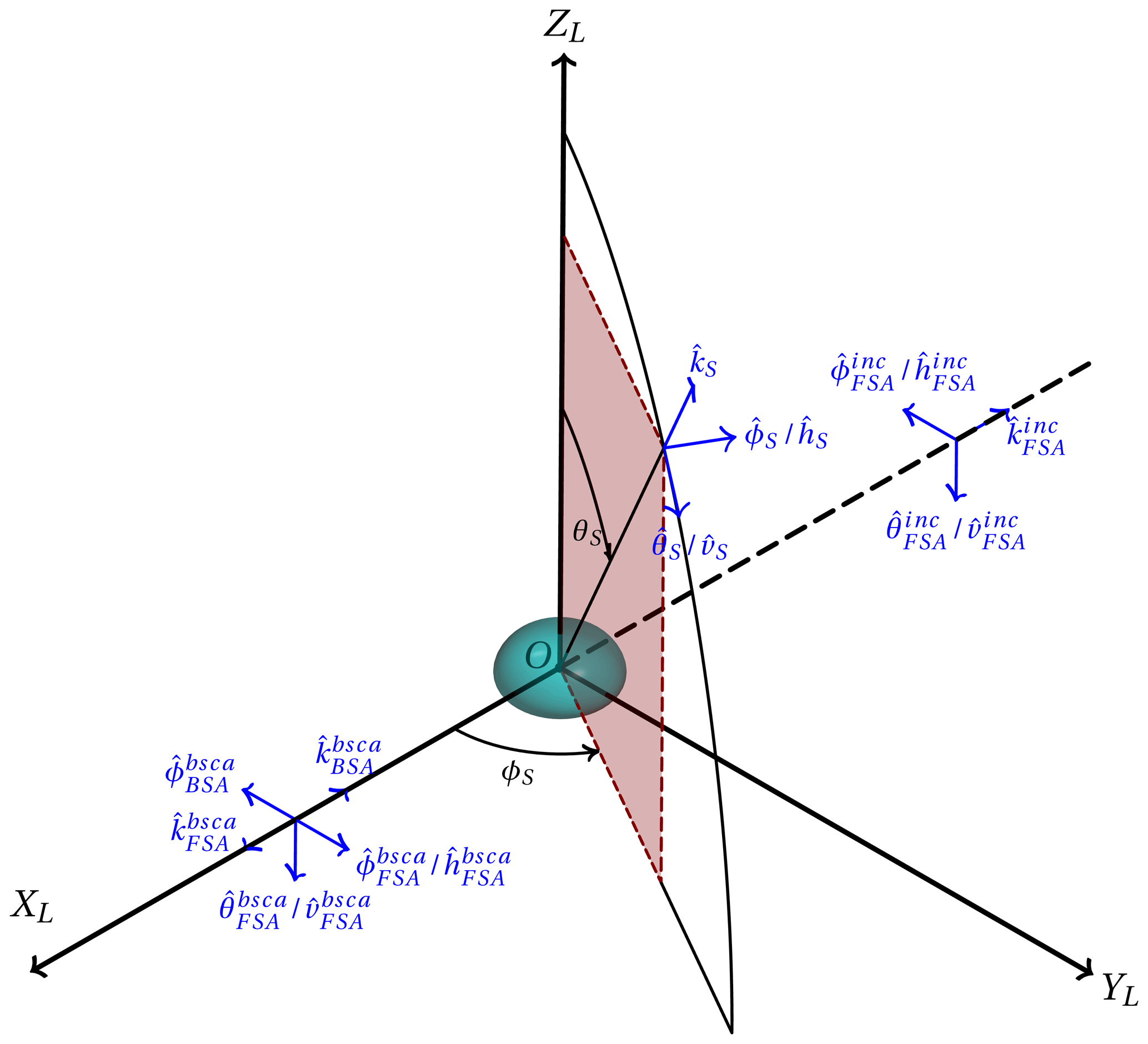
Figure C1 The unit vectors in the definition of the amplitude-scattering matrix. We assumed that the particle is located at the origin of the laboratory coordinate system and that the incident light propagated along the −X_L direction. The unit vectors subscripted with forward scattering alignment (FSA) are unit vectors defined in the FSA convention, while unit vectors defined by the back-scattering alignment (BSA) convention are indicated by the subscript BSA.

Appendix D: Calculations of radar variables

Next we describe how to perform intrinsic radar variable calculations using bulk matrices 〈Z〉 and 〈K〉:

1. Horizontal/vertical reflectivity $z_{\mathrm{h}/\mathrm{v}}$ (in units of mm⁶ m⁻³):

   $$\begin{array}{}\text{(D1)}& {\displaystyle }\begin{array}{l}{z}_{\mathrm{h}}=\frac{{\mathit{\lambda }}^{\mathrm{4}}}{{\mathit{\pi }}^{\mathrm{5}}\mathrm{|}{K}_{\mathrm{w}}{\mathrm{|}}^{\mathrm{2}}}\underset{\mathrm{0}}{\overset{\mathrm{\infty }}{\int }}{\mathit{\sigma }}_{\mathrm{bsca},\mathrm{h}}N\left(D\right)\mathrm{d}D,\\ =\frac{\mathrm{4}\mathit{\pi }{\mathit{\lambda }}^{\mathrm{4}}}{{\mathit{\pi }}^{\mathrm{5}}\mathrm{|}{K}_{\mathrm{w}}{\mathrm{|}}^{\mathrm{2}}}\underset{\mathrm{0}}{\overset{\mathrm{\infty }}{\int }}{\left|S_{\mathrm{hh}}\right|}^{\mathrm{2}}N\left(D\right)\mathrm{d}D,\\ =\frac{\mathrm{2}{\mathit{\lambda }}^{\mathrm{4}}}{{\mathit{\pi }}^{\mathrm{4}}\mathrm{|}{K}_{\mathrm{w}}{\mathrm{|}}^{\mathrm{2}}}\underset{\mathrm{0}}{\overset{\mathrm{\infty }}{\int }}(Z_{\mathrm{11}}-Z_{\mathrm{12}}-Z_{\mathrm{12}}+Z_{\mathrm{22}})N\left(D\right)\mathrm{d}D,\\ =\frac{\mathrm{2}{\mathit{\lambda }}^{\mathrm{4}}}{{\mathit{\pi }}^{\mathrm{4}}\mathrm{|}{K}_{\mathrm{w}}{\mathrm{|}}^{\mathrm{2}}}\left(〈Z_{\mathrm{11}}〉-〈Z_{\mathrm{12}}〉-〈Z_{\mathrm{21}}〉+〈Z_{\mathrm{22}}〉\right),\end{array}\text{(D2)}& {\displaystyle }{z}_{\mathrm{v}}={\displaystyle \frac{\mathrm{2}{\mathit{\lambda }}^{\mathrm{4}}}{{\mathit{\pi }}^{\mathrm{4}}\mathrm{|}{K}_{\mathrm{w}}{\mathrm{|}}^{\mathrm{2}}}}\left(〈Z_{\mathrm{11}}〉+〈Z_{\mathrm{12}}〉+〈Z_{\mathrm{21}}〉+〈Z_{\mathrm{22}}〉\right).\end{array}$$

   In Eq. (D1), σ_bsca,h indicates the horizontal backscattering cross section of a particle (i.e., ${\mathit{\sigma }}_{\mathrm{bsca},\mathrm{h}}=\mathrm{4}\mathit{\pi }{\left|S_{\mathrm{hh}}\right|}^{\mathrm{2}}$). λ is the wavelength of radar, $K_{\mathrm{w}}=\left|\left({\mathit{\epsilon }}_{\mathrm{w}}-\mathrm{1}\right)/\left({\mathit{\epsilon }}_{\mathrm{w}}+\mathrm{2}\right)\right|$ is the dielectric factor (ε_w is the dielectric constant of water at the wavelength of radar for a fixed temperature of 283.15 K). Similarly, vertical reflectivity can be derived in Eq. (D2).

2. Differential reflectivity z_dr (dimensionless):

   $$\begin{array}{}\text{(D3)}& z_{\mathrm{dr}}={\displaystyle \frac{z_{\mathrm{h}}}{z_{\mathrm{v}}}}={\displaystyle \frac{〈Z_{\mathrm{11}}〉-〈Z_{\mathrm{12}}〉-〈Z_{\mathrm{21}}〉+〈Z_{\mathrm{22}}〉}{〈Z_{\mathrm{11}}〉+〈Z_{\mathrm{12}}〉+〈Z_{\mathrm{21}}〉+〈Z_{\mathrm{22}}〉}}.\end{array}$$

3. The specific differential-phase shift (° km⁻¹) upon propagation, K_DP, is defined by

   $$\begin{array}{}\text{(D4)}& \begin{array}{l}{K}_{\mathrm{DP}}={\mathrm{10}}^{-\mathrm{3}}\cdot \frac{\mathrm{180}}{\mathit{\pi }}\cdot \mathit{\lambda }\underset{\mathrm{0}}{\overset{\mathrm{\infty }}{\int }}\mathfrak{R}(S_{\mathrm{hh}}^{\mathrm{fwd}}-S_{\mathrm{vv}}^{\mathrm{fwd}})N\left(D\right)\mathrm{d}D\\ ={\mathrm{10}}^{-\mathrm{3}}\cdot \frac{\mathrm{180}}{\mathit{\pi }}\cdot \underset{\mathrm{0}}{\overset{\mathrm{\infty }}{\int }}\frac{\mathrm{2}\mathit{\pi }}{k_{\mathrm{0}}}\mathfrak{R}(S_{\mathrm{hh}}^{\mathrm{fwd}}-S_{\mathrm{vv}}^{\mathrm{fwd}})N\left(D\right)\mathrm{d}D\\ ={\mathrm{10}}^{-\mathrm{3}}\cdot \frac{\mathrm{180}}{\mathit{\pi }}\cdot 〈K_{\mathrm{34}}〉.\end{array}\end{array}$$

   Here, 10⁻³ in Eq. (D4) represents the coefficient in the unit conversion (from mm² m⁻³ to km⁻¹), and the coefficient $\mathrm{180}/\mathit{\pi }$ is used to convert the unit of the result (from radii km⁻¹ to ° km⁻¹). Here, the superscripts of “fwd” over the matrix elements indicate that these are elements of the forward scattering matrix.

4. The one-way linear-scale attenuation coefficient⁵ of horizontal/vertical polarization $a_{\mathrm{h}/\mathrm{v}}$ (in units of km⁻¹):

   $$\begin{array}{}\text{(D5)}& {\displaystyle }\begin{array}{l}{a}_{\mathrm{h}}={\mathrm{10}}^{-\mathrm{3}}\underset{\mathrm{0}}{\overset{\mathrm{\infty }}{\int }}{\mathit{\sigma }}_{\mathrm{ext},\mathrm{h}}N\left(D\right)\mathrm{d}D\\ ={\mathrm{10}}^{-\mathrm{3}}\underset{\mathrm{0}}{\overset{\mathrm{\infty }}{\int }}\frac{\mathrm{4}\mathit{\pi }}{k_{\mathrm{0}}}\mathfrak{I}\left(S_{\mathrm{hh}}^{\mathrm{fwd}}\right)N\left(D\right)\mathrm{d}D\\ \\ ={\mathrm{10}}^{-\mathrm{3}}\underset{\mathrm{0}}{\overset{\mathrm{\infty }}{\int }}(K_{\mathrm{11}}-K_{\mathrm{12}})N\left(D\right)\mathrm{d}D\\ ={\mathrm{10}}^{-\mathrm{3}}\left(〈K_{\mathrm{11}}〉-〈K_{\mathrm{12}}〉\right)\end{array}\text{(D6)}& {\displaystyle }{a}_{\mathrm{v}}={\mathrm{10}}^{-\mathrm{3}}\left(〈K_{\mathrm{11}}〉+〈K_{\mathrm{12}}〉\right).\end{array}$$

   Again, 10⁻³ in Eq. (D5) serves as the coefficient (in unit the conversion from mm² m⁻³ to km⁻¹). σ_ext,h indicates horizontal extinction cross section of a given particle (i.e., ${\mathit{\sigma }}_{\mathrm{ext},\mathrm{h}}=\frac{\mathrm{4}\mathit{\pi }}{k_{\mathrm{0}}}\mathfrak{I}\left(S_{\mathrm{hh}}^{\mathrm{fwd}}\right))$. Similarly, vertical attenuation coefficient can be derived in Eq. (D6).

5. The total differential-phase shift upon backscattering δ_hv in units of degrees (hereafter deg.) is represented as shown below:

   $$\begin{array}{}\text{(D7)}& \begin{array}{l}{\mathit{\delta }}_{\mathrm{hv}}=\frac{\mathrm{180}}{\mathit{\pi }}\mathrm{\angle }\left(\underset{\mathrm{0}}{\overset{\mathrm{\infty }}{\int }}{S}_{\mathrm{hh}}{S}_{\mathrm{vv}}^{\ast }N\left(D\right)\mathrm{d}D\right)\\ =\frac{\mathrm{180}}{\mathit{\pi }}\mathrm{\angle }\left(\underset{\mathrm{0}}{\overset{\mathrm{\infty }}{\int }}\left[\mathrm{0.5}(Z_{\mathrm{33}}+Z_{\mathrm{44}})+\mathrm{0.5}(Z_{\mathrm{43}}-Z_{\mathrm{34}})i\right]N\left(D\right)\mathrm{d}D\right)\\ =\frac{\mathrm{180}}{\mathit{\pi }}\mathrm{\angle }\left(\left[〈Z_{\mathrm{33}}〉+〈Z_{\mathrm{44}}〉\right]+\left[〈Z_{\mathrm{43}}〉-〈Z_{\mathrm{34}}〉\right]i\right)\end{array}.\end{array}$$

   The notation “∠” in Eq. (D7) indicates the phase of the complex value. The coefficient $\mathrm{180}/\mathit{\pi }$ is used to convert the unit of the result from radii to deg.

6. Co-polar correlation coefficient ρ_hv (dimensionless):

   $$\begin{array}{}\text{(D8)}& \begin{array}{l}{\mathit{\rho }}_{\mathrm{hv}}=\frac{\left|\underset{\mathrm{0}}{\overset{\mathrm{\infty }}{\int }}{S}_{\mathrm{hh}}{S}_{\mathrm{vv}}^{\ast }N\left(D\right)\mathrm{d}D\right|}{\sqrt{\underset{\mathrm{0}}{\overset{\mathrm{\infty }}{\int }}{\left|S_{\mathrm{hh}}\right|}^{\mathrm{2}}N\left(D\right)\mathrm{d}D\cdot \underset{\mathrm{0}}{\overset{\mathrm{\infty }}{\int }}{\left|S_{\mathrm{vv}}\right|}^{\mathrm{2}}N\left(D\right)\mathrm{d}D}}\\ =\frac{\left|\underset{\mathrm{0}}{\overset{\mathrm{\infty }}{\int }}\left[\mathrm{0.5}(Z_{\mathrm{33}}+Z_{\mathrm{44}})+\mathrm{0.5}(Z_{\mathrm{43}}-Z_{\mathrm{34}})i\right]N\left(D\right)\mathrm{d}D\right|}{\sqrt{\begin{array}{c}{\int }_{\mathrm{0}}^{\mathrm{\infty }}\mathrm{0.5}(Z_{\mathrm{11}}-Z_{\mathrm{12}}-Z_{\mathrm{21}}+Z_{\mathrm{22}})N\left(D\right)\mathrm{d}D\\ \cdot {\int }_{\mathrm{0}}^{\mathrm{\infty }}\mathrm{0.5}(Z_{\mathrm{11}}+Z_{\mathrm{12}}+Z_{\mathrm{21}}+Z_{\mathrm{22}})N\left(D\right)\mathrm{d}D\end{array}}}\\ =\frac{\left|\left(〈Z_{\mathrm{33}}〉+〈Z_{\mathrm{44}}〉\right)+\left(〈Z_{\mathrm{43}}〉-〈Z_{\mathrm{34}}〉\right)i\right|}{\sqrt{\begin{array}{c}\left(〈Z_{\mathrm{11}}〉-〈Z_{\mathrm{12}}〉-〈Z_{\mathrm{21}}〉+〈Z_{\mathrm{22}}〉\right)\\ \cdot \left(〈Z_{\mathrm{11}}〉+〈Z_{\mathrm{12}}〉+〈Z_{\mathrm{21}}〉+〈Z_{\mathrm{22}}〉\right)\end{array}}}\end{array}.\end{array}$$

   In Eq. (D8), the co-polar correlation coefficient ρ_hv is the amplitude of complex co-polar correlation coefficient $\stackrel{\mathrm{̃}}{{\mathit{\rho }}_{\mathrm{hv}}}$, whose phase is the total differential-phase shift upon backscattering in Eq. (D7).

Please note that the summation over hydrometeor types was omitted in Eqs. (D1)–(D8) for the sake of clarity. Readers can easily obtain the more complicated, real expressions of radar variables by applying extra summations over hydrometeor types for 〈Z〉 and 〈K〉 elements before carrying out the calculations.

The aforementioned radar variables $z_{\mathrm{h}/\mathrm{v}}$, $a_{\mathrm{h}/\mathrm{v}}\left({\mathit{\alpha }}_{\mathrm{h}/\mathrm{v}}\right)$, z_dr, K_DP, δ_hv, and ρ_hv are often referred to as intrinsic radar variables determined by the atmosphere and hydrometeor conditions in local radar gates. Under the assumption of first-order multiple-scattering model, although the wave is scattered only once before it is received, the two-way propagation effects such as attenuation and phase shift are taken into account using the wave number of the effective medium composed of air and hydrometeors along the beam trajectory (Zhang, 2016). We can derive the observable radar variables as shown below:

$$\begin{array}{}\text{(D9)}& {\displaystyle }{z}_{\mathrm{h}/\mathrm{v}}^{\prime }\left(r_{\mathrm{g}}\right)=z_{\mathrm{h}/\mathrm{v}}\left(r_{\mathrm{g}}\right)\cdot \exp \left(-\mathrm{2}\underset{r=\mathrm{0}}{\overset{r=r_{\mathrm{g}}}{\int }}{a}_{\mathrm{h}/\mathrm{v}}\left(r\right)\mathrm{d}r\right),\text{(D10)}& {\displaystyle }{\mathrm{\Phi }}_{\mathrm{DP}}\left(r_{\mathrm{g}}\right)=\mathrm{2}\underset{r=\mathrm{0}}{\overset{r=r_{\mathrm{g}}}{\int }}{K}_{\mathrm{DP}}\left(r\right)\mathrm{d}r+{\mathit{\delta }}_{\mathrm{hv}}\left(r_{\mathrm{g}}\right).\end{array}$$

In Eqs. (D9) and (D10), r_g is the range of the radar gate, and the variable of integration r is the range along the radar beam trajectory. $z_{\mathrm{h}/\mathrm{v}}^{\prime }$ marked with a prime is the horizontal/vertical observable reflectivity of the radar gate attenuated on the way from the transmitter to the particle and on the way back from the particle to the receiver. Φ_DP is the total phase shift interpreted as the differential-phase shift upon two-way propagation plus the differential phase shift upon backscattering.

$$\begin{array}{}\text{(D11)}& {\displaystyle }{Z}_{\mathrm{H}/\mathrm{V}}^{\prime }=\mathrm{10}{\log }_{\mathrm{10}}\left(z_{\mathrm{h}/\mathrm{v}}^{\prime }\right),\text{(D12)}& {\displaystyle }{Z}_{\mathrm{DR}}^{\prime }=\mathrm{10}{\log }_{\mathrm{10}}\left(z_{\mathrm{dr}}^{\prime }\right)=\mathrm{10}{\log }_{\mathrm{10}}\left({\displaystyle \frac{z_{\mathrm{h}}^{\prime }}{z_{\mathrm{v}}^{\prime }}}\right).\end{array}$$

Equations (D11) and (D12) give the observable horizontal/vertical reflectivity $Z_{\mathrm{H}/\mathrm{V}}^{\prime }$ (in units of dBZ) and differential reflectivity $Z_{\mathrm{DR}}^{\prime }$ (in units of dB).