the Creative Commons Attribution 4.0 License.
the Creative Commons Attribution 4.0 License.
 | 24 Jul 2024
Evaluating CHASER V4.0 global formaldehyde (HCHO) simulations using satellite, aircraft, and ground-based remote-sensing observations
Hossain Mohammed Syedul Hoque
Kengo Sudo
Hitoshi Irie
Yanfeng He
Md Firoz Khan
Formaldehyde (HCHO), a precursor to tropospheric ozone, is an important tracer of volatile organic compounds (VOCs) in the atmosphere. Two years (2019–2020) of HCHO simulations obtained from the global chemistry transport model CHASER at a horizontal resolution of 2.8° × 2.8° have been evaluated using the Tropospheric Monitoring Instrument (TROPOMI) and multi-axis differential optical absorption spectroscopy (MAX-DOAS) observations. In situ measurements from the Atmospheric Tomography Mission (ATom) in 2018 were used to evaluate the HCHO simulations for 2018. CHASER reproduced the TROPOMI-observed global HCHO spatial distribution with a spatial correlation (r) of 0.93 and a negative bias of 7 %. The model showed a good capability to reproduce the observed magnitude of the HCHO seasonality in different regions, including the background conditions. The discrepancies between the model and satellite in the Asian regions were related mainly to the underestimated and missing anthropogenic emission inventories. The maximum difference between two HCHO simulations based on two different nitrogen oxide (NOx) emission inventories was 20 %. TROPOMI's finer spatial resolution than that of the Ozone Monitoring Instrument (OMI) sensor reduced the global model–satellite root-mean-square error (RMSE) by 20 %. The OMI- and TROPOMI-observed seasonal variations in HCHO abundances were consistent. The simulated seasonality showed better agreement with TROPOMI in most regions. The simulated HCHO and isoprene profiles correlated strongly (R=0.81) with the ATom observations. However, CHASER overestimated HCHO mixing ratios over dense vegetation areas in South America and the remote Pacific region (background condition), mainly within the planetary boundary layer (< 2 km). The simulated seasonal variations in the HCHO columns showed good agreement (R>0.70) with the MAX-DOAS observations and agreed within the 1σ standard deviation of the observed values. However, the temporal correlation (R∼0.40) was moderate on a daily scale. CHASER underestimated the HCHO levels at all sites, and the peak occurrences in the observed and simulated HCHO seasonality differed. The coarseness of the model's resolution could potentially lead to such discrepancies. Sensitivity studies showed that anthropogenic emissions were the highest contributor (up to ∼ 35 %) to the wintertime regional HCHO levels.
- Article
(4232 KB) - Full-text XML
-
Supplement
(2149 KB) - BibTeX
- EndNote


Formaldehyde (HCHO), the most abundant carbonyl compound in the atmosphere, is a high-yield oxidation product of all primary biogenic and anthropogenic non-methane volatile organic compounds (NMVOCs). Methane (CH4) oxidization produces background HCHO concentrations of 0.2–1.0 ppbv (Burkert et al., 2001; Singh et al., 2004; Sinreich et al., 2005; Weller et al., 2000). Along with secondary sources (i.e., the oxidization of NMVOCs), biomass burning, industrial processes, and fossil fuel combustion are the primary HCHO emission sources (Fu et al., 2008; Hak et al., 2005; Lee et al., 1997). However, the oxidization of NMVOCs drives the spatial variability of HCHO on a global scale (Franco et al., 2015). HCHO removal mechanisms include photolysis at wavelengths below 400 nm, oxidization by hydroxyl radicals (OH), and wet deposition. The atmospheric lifetime of HCHO is around a few hours (Arlander et al., 1995). Therefore, HCHO observations can help elucidate chemical processes in the atmosphere. A few examples are the following: (1) the ozone (O3) production regime can be determined from the HCHO to nitrogen dioxide (NO2) ratio (Duncan et al., 2010; Hoque et al., 2022; Martin et al., 2004); (2) midday OH levels can be quantified from the oxidation of isoprene into HCHO (Kaiser et al., 2015); and (3) HCHO, being an intermediate product in the oxidation chain of NMVOCs, engenders the formation of carbon monoxide (CO) and carbon dioxide (CO2). Consequently, CO chemical production from NMVOCs and CH4 can be quantified from HCHO measurements (De Smedt et al., 2021).
Given its importance, global HCHO observations started in 1995 with the launch of a nadir-viewing ultraviolet (UV) sensor, the Global Ozone Monitoring Experiment (GOME; Burrows et al., 1999). Since then, there have been numerous sensors: the SCanning Imaging Absorption SpectroMeter for Atmospheric CHartographY (SCIAMACHY; De Smedt et al., 2008, 2010; Wittrock et al., 2006) on board the ENVISAT satellite, the Ozone Monitoring Instrument (OMI) (Levelt et al., 2018), the Global Ozone Monitoring Experiment-2 (GOME-2) (Munro et al., 2016), and the Ozone Mapping and Profiler Suite (González Abad et al., 2016, new reference). The HCHO observations from these sensors have been used extensively to evaluate models, air quality, and climate change (Chutia et al., 2019; De Smedt et al., 2008, 2010, 2015; Hoque et al., 2022). The Tropospheric Monitoring Instrument (TROPOMI) (De Smedt et al., 2021; Veefkind et al., 2012), launched on the European Copernicus Sentinel-5 Precursor (S5P) satellite on 13 October 2017, is a recent addition to the series of nadir-viewing UV sensors providing HCHO data. The unprecedented original spatial resolution of 3.5 × 7 km2 (across track × along track), which was refined to 3.5 × 5.5 km2 on 6 August 2019, is the crucial feature of TROPOMI. Such spatial resolution is almost 16 times finer than its predecessor, OMI (De Smedt et al., 2021). Such high-resolution observations will likely reduce uncertainties in the HCHO products for multiple research purposes.
Several studies that used the TROPOMI HCHO product have been reported in the literature. De Smedt et al. (2021) and Vigouroux et al. (2020) have validated TROPOMI HCHO comprehensively against the MAX-DOAS and FTIR networks. Both studies have concluded that TROPOMI HCHO products have achieved the pre-launch accuracy requirement of < 40 %–80 %. Ryan et al. (2020) and Chan et al. (2020) reported good agreement (temporal correlation R>0.70) between TROPOMI and MAX-DOAS in Melbourne and Munich. In addition to validation studies, HCHO products have been used to infer changes in the global HCHO levels during the shutdown prompted by the COVID-19 pandemic (Levelt et al., 2022; Souri et al., 2021; Sun et al., 2021), demonstrating the role of anthropogenic emissions in global HCHO variability.
Among the multitude of applications of TROPOMI HCHO observations, few efforts have specifically evaluated HCHO simulations from global chemistry transport models (CTMs). This work evaluates the HCHO spatiotemporal distribution simulated by the global Chemical Atmospheric General Circulation Model for the Study of Atmospheric Environment and Radiative Forcing (CHASER) (Sekiya and Sudo, 2014; Sudo et al., 2002; Sudo and Akimoto, 2007) against TROPOMI HCHO observations. In addition, airborne and ground-based observations are used to validate the simulated HCHO profiles and surface mixing ratios in a few regions. CHASER simulations of NO2, OH, and O3 have been evaluated against satellite and ground-based observations (e.g., Sekiya and Sudo, 2014; Sekiya et al., 2018). Moreover, CHASER is a forward model in the chemical reanalysis system (TCR) developed by Miyazaki et al. (2017, 2020). The model simulations are performed at a horizontal resolution of 2.8° × 2.8° (T42). Although the model can run at higher resolutions, T42 is the most commonly used framework for CHASER applications. Therefore, it is used for this study.
Hoque et al. (2022) validated CHASER-simulated NO2 and HCHO against OMI and MAX-DOAS observations for 2017. CHASER showed good skills in reproducing the HCHO abundances observed by OMI (spatial correlation r=0.74) and MAX-DOAS (temporal correlation R>0.80). The study found that biomass burning contributes ∼ 50 % to the HCHO levels observed at the site in Thailand. However, the limitations of the study were that (1) the simulated HCHO partial column and profile were evaluated against MAX-DOAS observations on a seasonal scale only, (2) the model sensitivity studies were site specific and thus did not provide global statistics on the emission contribution, and (3) satellite observations were used as supporting datasets, so the model–satellite comparison was not comprehensive. This study utilizes multi-satellite (TROPOMI and OMI) HCHO observations, different NOx emission inventories, aircraft measurements, and daily and diurnal MAX-DOAS data to provide robust and comprehensive statistics on the model HCHO simulations.
2.1 CHASER
CHASER V4.0 (version 4) is a global CTM that studies the atmospheric environment and radiative forcing. It is coupled online with the MIROC atmospheric general circulation model (AGCM) and the SPRINTAS aerosol transport model (Takemura et al., 2005, 2009). The latest version of CHASER (Ha et al., 2023; He et al., 2022) entails several updates, including those related to the formation of aerosol species and related chemistry, radiation, and cloud processes.
Through 263 multi-phase (gaseous, aqueous, and heterogeneous) chemical reactions, CHASER calculates the concentrations of 92 species by considering the chemical cycle involving O3, NOx (nitrogen oxides), HOx (hydrogen oxides), and CH4-CO along with the oxidation of NMVOCs (Ha et al., 2023; He et al., 2022; Hoque et al., 2022; Miyazaki et al., 2017; Sekiya et al., 2023). The chemical mechanism adopted comes mainly from the master chemical mechanism (MCM) (Jenkin et al., 2015). The stratospheric O3 chemistry simulations are based on the Chapman mechanism, the catalytic reaction of halogen oxides, and polar stratospheric clouds. The dry and wet depositions are calculated based on resistance-based parameterization (Wesley et al., 2007), cumulus convection, and large-scale condensation parameterization. Advective trace transport is calculated using the piecewise parabolic method (Colella and Woodward, 1984) and flux-form semi-Lagrangian schemes. Tracer transport is simulated on a sub-grid scale in the framework of the prognostic Arakawa–Schubert cumulus convection scheme (Emori et al., 2001) and a vertical diffusion scheme (Mellor and Yamada, 1974). The simulations were performed at a horizontal resolution of 2.8° × 2.8°, employing 36 vertical layers from the surface to approx. 50 km altitude and a 20 min time step. At every time step, meteorological fields obtained from the MIROC AGCM were nudged toward the 6-hourly NCEP FNL reanalysis data.
CHASER incorporates emissions from biomass burning, anthropogenic sources, lightning, and soil. Anthropogenic NOx emissions for 2018 are obtained from the HTAP_v3 inventory (Crippa et al., 2023). Other anthropogenic emissions are taken from HTAP_v2.2 for 2008, and the biomass burning emissions are from MACC-GFAS (Inness et al., 2013). The monthly soil NOx emissions, derived from Yienger and Levy (1995), are constant across years. Biogenic emissions of VOCs are obtained from a process-based biogeochemical model: the Vegetation Integrative SImulator for Trace gases (VISIT) (Ito and Inatomi, 2012). VISIT is part of the CHASER modeling framework and incorporates the biogenic flux estimate scheme of Guenther (1997) (Ito et al., 2012). The global isoprene emissions in VISIT and the CAMS global biogenic emission inventory (Sinderolova et al., 2022; based on MEGANv2.1) are 400 and 450 Tg C yr−1, respectively. Lightning NOx production estimates are based on the parameterization of Price and Rind (1992) and linked to the convection scheme of the AGCM. Global NOx emissions in CHASER are set to 43.80 Tg N yr−1, with industrial production (23.10 Tg N yr−1), biomass burning (9.65 Tg N yr−1), soil (5.50 Tg N yr−1), lightning (5 Tg N yr−1), and aircraft (0.55 Tg N yr−1) considered as significant emission sources. Annual monoterpene, acetone, and other non-methane volatile organic compound (ONMV) emissions are 102, 20, and 60 Tg C yr−1, respectively. Direct emissions of HCHO from anthropogenic sources and biomass burning are not considered in CHASER. However, secondary production of HCHO from VOCs (C2H6, C3H8, C2H4, C3H6, CH3COCH3, and ONMV) emitted directly from anthropogenic and pyrogenic sources is considered.
Sekiya et al. (2018) comprehensively assessed CHASER-simulated NO2 abundances using OMI observations. CHASER reproduced the ATom-observed OH spatiotemporal variation well (Sekiya et al., 2018). The quality of O3 simulations has been explained in the work of Sudo et al. (2007). Ha et al. (2023) and He et al. (2022) updated the heterogeneous chemistry and lightning NOx schemes, respectively. These updates have not been considered in the current study. The effect of these updates on the HCHO simulations will be addressed in a separate study. Multiple simulations with varying emission inputs were performed for the study. They are presented in Table 1.
Table 1Combinations of emission inventories used in the different simulations used in this study.
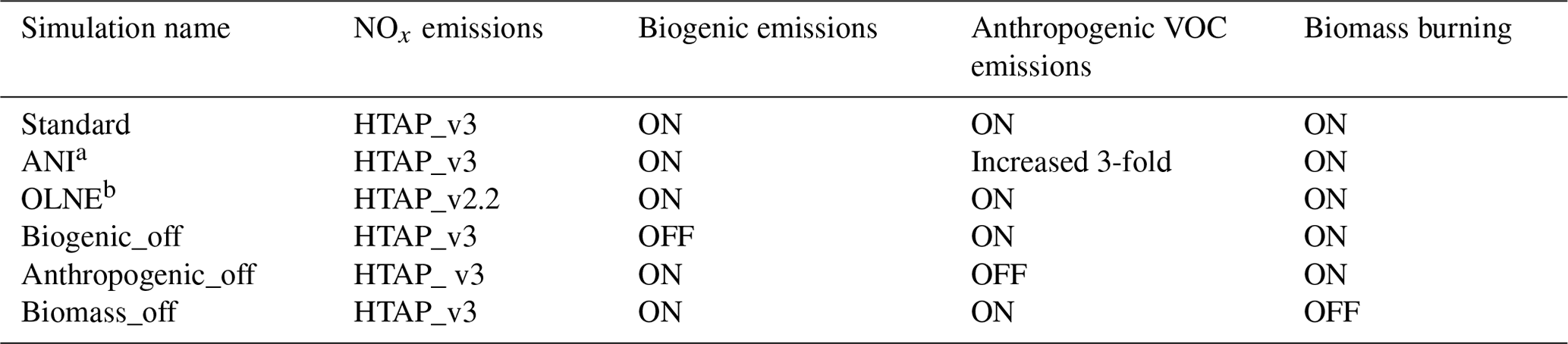
a Anthropogenic VOC emissions were increased 3-fold in ANI. b The OLNE simulation used old NOx emissions.
To account for the altitude dependence of TROPOMI observations, averaging kernel (AK) information obtained from the level (L2) files was applied to all simulations, following the method of Sekiya et al. (2018). First, the simulated HCHO profiles were sampled closest to the TROPOMI overpass of 13:30 LT (local time). Secondly, AKs averaged on a 2.8° bin grid were applied to the sampled profiles. Then, the total column was calculated. Thirdly, the AK-applied model columns on the available measurement days were selected.
2.2 TROPOMI
The TROPOMI operational L2 offline (OFFL) HCHO vertical column density (VCD) (ver. 1.1.5.7) data from 2019 to 2020 have been used for this study. The S5P TROPOMI HCHO L2 product user manual (Veefkind et al., 2012) provides a detailed product description. The TROPOMI HCHO retrieval algorithm is based on the DOAS technique and was adapted directly from the OMI QA4ECV product retrieval algorithm (De Smedt et al., 2017). The three-step retrieval algorithm was explained explicitly by De Smedt et al. (2018). Slant columns were retrieved from the UV part of the spectra (channel 3) in the 328.5–358 nm fitting window. The HCHO cross-section data reported by Meller and Moortgart (2000) were used to fit the spectra. All the cross-sections were convolved with the instrument's slit function (adjusted after the launch) for every row separately. Spectra averaged over the tropical Pacific region from the prior day were used as reference spectra for the DOAS fit (De Smedt et al., 2021; Vigouroux et al., 2020). The slant columns, therefore, exceed the average Pacific background HCHO levels because they were derived from the differences between the local and reference spectra. The slant columns were converted to tropospheric columns (Nv) using a lookup table of vertically resolved air mass factors (M) at 340 nm calculated with the radiative transfer model VILDORT v2.6 (Spurr, 2008). The value of M depends on the observation geometry, surface albedo, cloud properties, and a priori profiles of HCHO. The surface albedo at a spatial resolution of 1° × 1° was extracted from the monthly OMI albedo climatology (Kleipool et al., 2008). Daily HCHO profiles were obtained a priori from the TM5-MP CTM at a similar spatial resolution. The independent-pixel approximation (Boersma et al., 2004) approach was applied to pixels with cloud fractions greater than 0.1. Background correction was performed based on HCHO slant columns over the Pacific Ocean from the 5 days prior to account for any remaining global offsets and stripes (De Smedt et al., 2021). The background HCHO contribution from CH4 oxidation in the reference region was calculated with TM5-MP. The resulting HCHO tropospheric column was calculated using Eq. (1):
where Mo is the air mass factor of the reference sector. Following De Smedt et al. (2021), the following filters ensured the data quality: (1) a cloud fraction of less than 0.3, (2) quality assurance values of greater than 0.5, (3) retrievals with a solar zenith angle (SZA) of less than 70°, (4) a surface albedo of less than 0.1, and (5) an air mass factor of greater than 0.1. The total uncertainty in the reprocessed TROPOMI HCHO columns was estimated as ≥ 90 % for the fire-free region (Zhao et al., 2022, and references therein). The uncertainties in the air mass factors, slant column fitting, and background HCHO, respectively, account for 75 %, 25 %, and 40 % of the total uncertainty. The estimated uncertainty in the retrievals in regions with strong fires is ∼ 35 %. The filtering criteria for the TROPOMI datasets are as follows: quality assurance value (QA) > 0.6, solar zenith angle < 70°, cloud fraction < 0.3, air mass factor (AMF) > 0.1, and surface reflectivity < 0.2.
TROPOMI observations are averaged spatially and temporally on the CHASER grid (T42), leading to horizontal representativeness errors. However, the random horizontal representativeness errors are on the order of 5 %–10 %, which is lower than the individual retrieval error of the satellite observations (Boersma et al., 2016). If the model's horizontal resolution is increased by 50 % (i.e., simulated at a horizontal resolution of 1.4° × 1.4°), the change in HCHO abundances is less than 6 % (Fig. S1 and Table S1 in the Supplement). The vertical sensitivity of the satellite retrievals is the most relevant source of representativeness error (Boersma et al., 2016). The current study utilizes the TROPOMI AK information to minimize the representativeness error. Therefore, the horizontal representativeness error will likely affect the results less than other error sources, such as uncertainties in satellite retrieval, emission inventories, and model chemical mechanisms.
2.3 OMI
The comparison study used HCHO retrievals from OMI, a nadir-viewing spectrometer on board the Aura satellite, which measures backscattering solar radiation in the spectral range of 270–500 nm (Levelt et al., 2018). OMI crosses the Equator at 13:40 LT (Zara et al., 2018) and provides daily global coverage of trace gases, including HCHO, at a spatial resolution of 13 × 24 km2. HCHO columns from 2019 to 2020 retrieved using BIRA-IASBv14 (De Smedt et al., 2021) were obtained from the Aeronomie website (i.e., https://www.temis.nl/qa4ecv/hcho/hcho_omi.php, last access: 1 July 2023) for use in this study. The data-filtering criteria were cloud fraction < 0.3, SZA < 70°, quality flag = 0, and cross-track quality flag = 0. Like the TROPOMI data, the OMI data were also averaged spatially and temporally on the model grid (T42).
2.4 ATom-4 aircraft campaign
The NASA Atmospheric Tomography (ATom) mission used a DC-8 aircraft to study the remote atmosphere over the Pacific and Atlantic oceans from ∼ 80° N to ∼ 65° S (Wofsy et al., 2018). Repeated flights measured the vertical profiles from 0.15 to 12 km to provide information related to greenhouse gases, reactive and tracer species, and aerosol composition and size distribution (Kupc et al., 2018). Over 2 years and four phases, sampling was conducted in one of the four seasons in each stage (Zhao et al., 2022). Here, the 1 min averaged measurements of HCHO and isoprene during the ATom-4 flight (Fig. S2) in 2018 are used for the model evaluation. The NASA In Situ Airborne Formaldehyde (ISAF) instrument (Cazorla et al., 2015) performed HCHO sampling based on the laser-induced fluorescence technique. Isoprene was measured using two instruments: (a) The University of Irvine Whole Air Sampler (WAS) and (b) the National Center for Atmospheric Research (NCAR) Trace Organic Gas Analyzer (TOGA). WAS sampled the air every 3–5 min, with subsequent analyses performed in the laboratory using gas chromatography (Simpson et al., 2020). TOGO sampling was conducted every 2 min with a 35 s integrated sampling time (Apel et al., 2021). The uncertainties in the WAS and TOGA isoprene observations are, respectively, ±10 % and 15 %. The measurement uncertainty in HCHO was reported as 10 %. The simulations have been interpolated to the observed spatial and temporal resolutions following the method of He et al. (2022). The observed and interpolated HCHO and isoprene vertical profiles were averaged over a 300 m bin. The Atom campaign took place between 2016 and 2018.
2.5 MAX-DOAS observations
HCHO columns and the volume mixing ratio (vmr) were retrieved from 2 years of (2019–2020) MAX-DOAS observations at Phimai (15.18° N, 102.46° E, 212 m a.s.l.), Chiba (35.62° N, 140.10° E, 21 m a.s.l.), and Kasuga (33.52° N, 130.47° E, 28 m a.s.l.). The MAX-DOAS observations were conducted within the framework of the International Air Quality and Sky Research Remote Sensing (A-SKY) network (Irie, 2021). The sites were selected because continuous measurements from 2019 to 2020 were available for these sites. Phimai is a rural site in Thailand and experiences a biomass burning influence from January to April. The climate is divided into two seasons: (1) the dry season (January to May) and (2) the wet season (June to December). Chiba and Kasuga are urban sites in central and southern Japan, respectively. The seasonal classification at these sites is as follows: spring is from March to May, summer is from June to August, autumn is from September to November, and winter is from December to February. The observations at these sites are described elsewhere (i.e., Hoque et al., 2018a; Irie et al., 2011, 2015).
The A-SKY MAX-DOAS system, including the instrument and algorithm, participated in the Cabauw Intercomparison campaign for Nitrogen Dioxide measuring Instruments (CINDI) and CINDI-2 (Kreher et al., 2020; Roscoe et al., 2010). The instrumentation has been described explicitly by Irie et al. (2008, 2011, 2015). A UV spectrometer (Maya2000Pro; Ocean Insight, Inc.) recorded high-resolution spectra from 310–515 nm at six elevation angles (ELs) of 2, 3, 4, 6, 8, and 70°, which were recorded every 15 min. The reference spectra were recorded at an EL of 70° instead of 90° to avoid saturation intensity. Spectra measured at all ELs were considered in the retrieved vertical profile and total columns. Consequently, the choice of reference ELs has no appreciable effect on the retrieval. The systematic error in the oxygen collision complex (O4) was reduced by limiting the off-axis ELs to less than 10° (Irie et al., 2015). However, this limitation reduces sensitivity above the planetary boundary layer (PBL), maintaining high sensitivity in the lower layers of the retrieved profiles. The high-resolution solar spectrum measured by Kurucz et al. (1984) was used for daily wavelength calibration. The spectral resolution is approximately 0.4 nm at 357 and 476 nm (Hoque et al., 2022). Aerosol and trace-gas columns and profiles were retrieved using the Japanese vertical-profile retrieval algorithm JM2 (ver. 2) (Irie et al., 2011, 2015). Three-step profile and column retrievals by JM2 are explained explicitly in earlier reports (e.g., Hoque et al., 2018a; Irie et al., 2011, 2015). The partial VCD values are converted to the volume mixing ratio (vmr) by scaling the US Standard Atmosphere temperature and pressure data to the surface measurements at the respective site. The estimated total error (random and systematic) in the HCHO product is 30 % (Hoque et al., 2022). Following Irie et al. (2011) and Hoque et al. (2018a, 2022), cloud screening was performed to ensure data quality.
3.1 Comparison of CHASER HCHO with TROPOMI observations
Figure 1 presents a comparison of the global distributions of annual mean HCHO columns obtained from TROPOMI retrievals and standard CHASER simulations at the TROPOMI overpass time (13:30 LT). Differences between the observations and model simulations in the respective years are also depicted. The statistics related to the comparison are presented in Table 2. The simulation results agree well with the TROPOMI observations, with a global spatial correlation (r) of 0.93, a mean bias error (MBE) (CHASER−TROPOMI) of −0.20 × 10¹⁵ molec. cm−2, and a root-mean-square error (RMSE) of 0.75×10¹⁵ molec. cm−2. The r, MBE, and RMSE values between 60° S and 60° N were, respectively, 0.92, 0.13×10¹⁵ molec. cm−2, and 0.82 × 10¹⁵ molec. cm−2. CHASER HCHO columns are negatively biased relative to the TROPOMI retrievals. Table S2 shows the MBE and RMSE values obtained for the individual months. No seasonal variation in the systematic differences between CHASER and TROPOMI was observed. Biases can originate from uncertainties in the retrieval and model assumptions. TROPOMI HCHO retrievals greater than 8 × 10¹⁵ molec. cm−2 were negatively biased by 25 % relative to the ground-based MAX-DOAS observations (De Smedt et al., 2021), whereas direct emissions of HCHO were not considered in CHASER. TROPOMI and CHASER show high HCHO concentrations over South America, central Africa, India, eastern China, and Southeast Asia. Simulated HCHO magnitudes in the hotspot regions were 0.8–1.4 × 10¹⁶ molec. cm−2, slightly higher than the observed range of 0.8–1 × 10¹⁶ molec. cm−2. The dataset's greatest differences (∼ 4 × 10¹⁵ molec. cm−2) were observed over Brazil and Southeast Asia. The datasets show a strong congruence in the high-latitude regions. The simulated and observed HCHO columns over Europe, the Middle East, Japan, and Russia were 0.3–0.6 × 10¹⁶ molec. cm−2. Simulated HCHO columns (∼ 3 × 10¹⁵ molec. cm−2) over the remote Pacific region were consistent with the observations, too. The remote Pacific region represents background conditions that are strongly linked to CH4 oxidation. The congruence with observations in this region suggests that the simulated CH4 estimates in remote areas are reasonable.
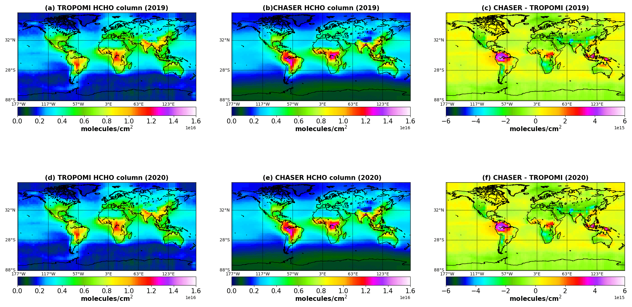
Figure 1Annual mean HCHO columns (×1016 molec. cm−2) in 2019 and 2020 obtained from TROPOMI retrievals (first column) and a standard CHASER simulation (second column). The differences between the model and observations in the respective years are shown in the third column. The unit of difference is × 1015 molec. cm−2.
Table 2Comparison of annual mean HCHO (× 1016 molec. cm−2) columns from TROPOMI retrievals and CHASER simulations for 2019 and 2020. MBE and RMSE are the abbreviations for mean bias error and root-mean-square error, respectively. The units of MBE and RMSE are × 1015 molec. cm−2. “Correlation” signifies the spatial correlation between the datasets.
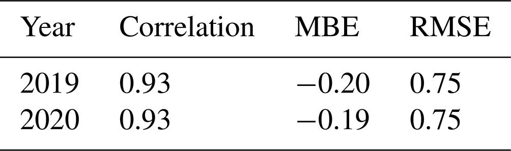
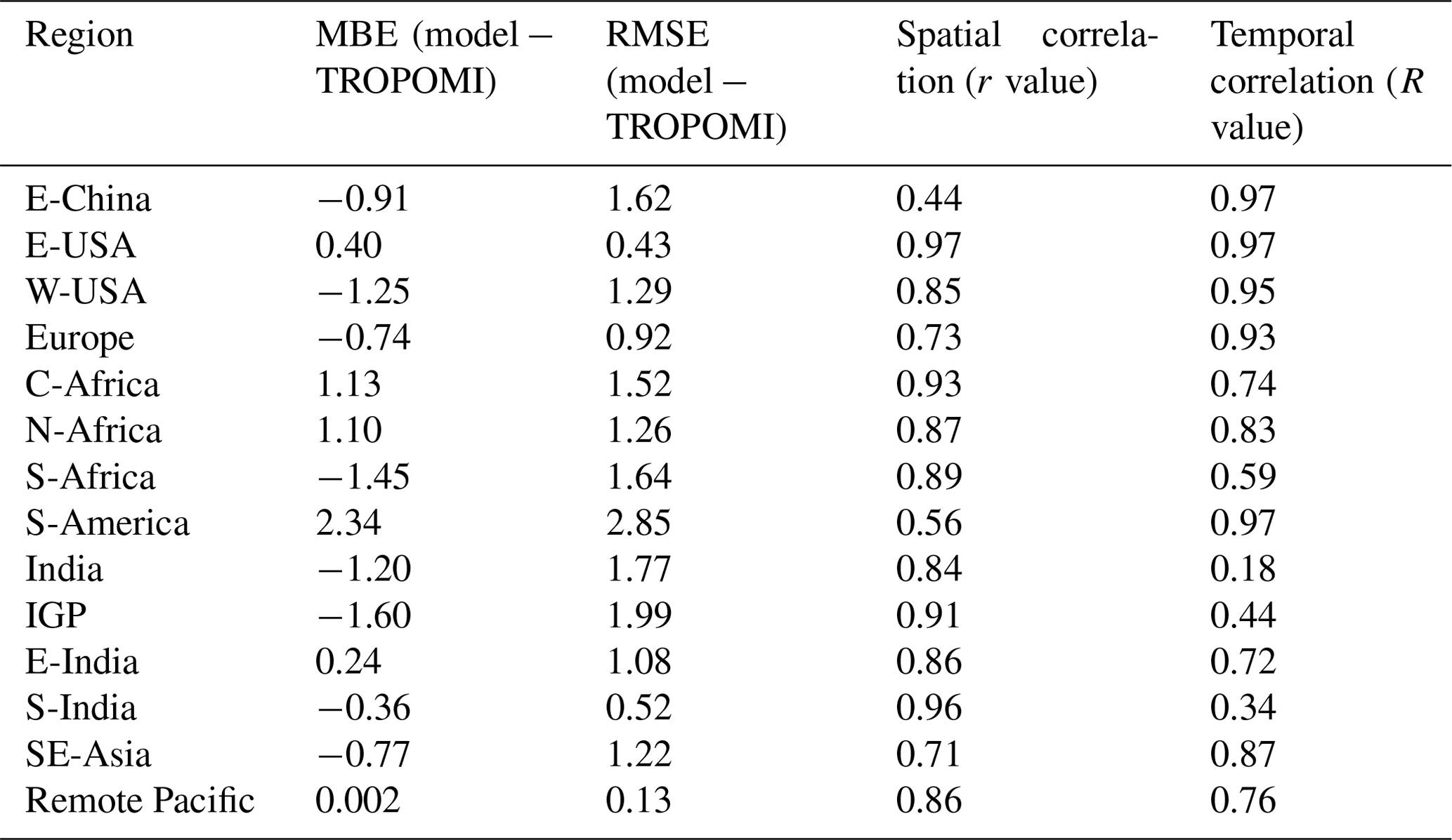
Figure 2 compares the observed and simulated seasonality in HCHO columns (×1016 molec. cm−2) in different regions. Datasets for 2019 and 2020 were used to calculate the observed and simulated monthly mean values. The MBE (×1015 molec. cm−2) between the TROPOMI and CHASER HCHO columns in each region is shown in blue. The comparison statistics are given in Table 3. The regional boundaries are shown on the global distribution map in Fig. S3. Temporal correlations derived from daily values over 2 years are provided in Table S2.
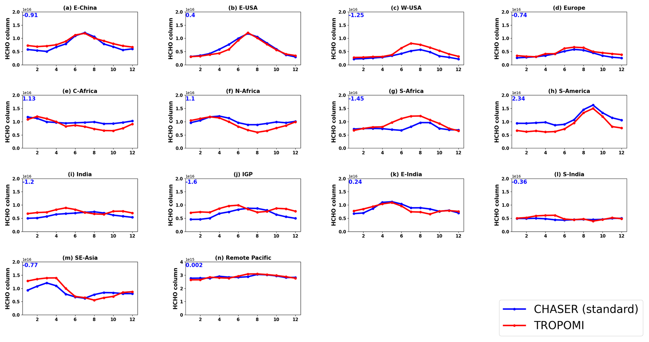
Figure 2Seasonal variation in HCHO columns (×1016 molec. cm−2) in (a) eastern China (E-China; 30–40° N, 110–123° E), (b) the eastern United States (E-USA; 32–43° N, 95–71° W), (c) the western United States (W-USA; 32–43° N, 125–100° W), (d) Europe (35–60° N, −10° W–30° E), (e) central Africa (C-Africa; 4° S–5° N, 10–40° E), (f) northern Africa (N-Africa; 5–15° N, 10° W–30° E), (g) southern Africa (S-Africa; 5–15° S, 10–30° E), (h) South America (S-America; 20° S–0° N, 50–70° W), (i) India (7.5–35° N, 68–89° E), (j) the Indo-Gangetic Plain (IGP; 21–33° N, 72–89° E), (k) east India (E-India; 15–25° N, 80–90° E), (l) south India (S-India; 0–15° N, 63–80° E), (m) Southeast Asia (SE-Asia, 10–20° N, 96–105° E), and (n) the remote Pacific region (28° S–32° N, 117–177° W), as inferred from CHASER simulations (blue) and TROPOMI observations (red). Blue numbers denote MBE between the TROPOMI and CHASER HCHO columns. The observed and simulated mean values represent the average of 2019 and 2020.
3.1.1 Eastern China
Over eastern China (E-China; Fig. 2a), the datasets are moderately correlated spatially (r=0.44), with MBE and RMSE values of −0.9 and 1.62 × 10¹⁵ molec. cm−2, respectively. The simulated seasonality correlates strongly with the observations (R=0.97), with a consistent peak (1×10¹⁶ molec. cm−2) in the HCHO variability in July. The HCHO column peaks are compatible with the peak in isoprene concentrations (Fig. S4), indicating a strong biogenic contribution during summer. CHASER mostly underestimated the wintertime HCHO columns in this region. Liu et al. (2021) reported vehicular exhaust, solvent usage, and combustion-related regional transport as the primary VOC emission sources during winter in Shanghai, a megacity in eastern China. NMVOC emissions from these sources (i.e., vehicular exhaust, solvent usage, and transport) are considered in the HTAP_v2.2 inventory (Crippa et al., 2023). Although CHASER considered HCHO production from the degradation of anthropogenic VOCs, it is likely underestimated, resulting in a lower simulated wintertime HCHO column in this region.
Table 3Comparison of monthly mean tropospheric HCHO (×1016 molec. cm−2) columns obtained from TROPOMI retrievals and standard CHASER simulations. Coincident dates in 2019 and 2020 are used to calculate the statistics. The units of MBE and RMSE are × 1015 molec. cm−2. The temporal correlations are derived from the seasonal means.
3.1.2 Eastern USA, western USA, and Europe
CHASER has reproduced the HCHO spatial variability in the eastern USA (E-USA; Fig. 2b; r=0.97) and western USA (W-USA; Fig. 2c; r=0.85) well. The peaks in the HCHO variability coincide with the isoprene peak in these regions (Fig. S4). The simulated amplitudes of the HCHO seasonal modulation in E-USA and W-USA are 74 % and 62 %, whereas the observed seasonal amplitudes are 74 % and 65 %, respectively. The peak in the HCHO seasonality in E-USA is similar in both datasets (∼ 1.2 × 10¹⁶ molec. cm−2). The RMSE value in the W-USA region is 15 % higher than that in E-USA. Although the spatial correlation in Europe (Fig. 2d) is moderate (r=0.73), the temporal correlation is strong (R=0.95). The simulated and observed HCHO seasonal modulations in Europe are 60 % and 62 %, respectively. The model–satellite discrepancies are prominent in Europe and W-USA during summer and autumn. In both regions (i.e., Europe and W-USA), the biogenic and anthropogenic contributions to the total HCHO level are equivalent during summer. In autumn, the anthropogenic emission contributions are higher (Sect. 3.8). This indicates a potential model underestimation of biogenic HCHO levels in these regions, linked to the uncertainties in the biogenic emission inventory and isoprene mechanism. However, the model–satellite agreement is strong during the winter in these regions. During winter, anthropogenic VOC emissions drive the HCHO variability in these regions (Luecken et al., 2018; Pozzani et al., 2002). Therefore, the simulated contribution of anthropogenic sources to the HCHO abundances during winter in these regions is reasonable.
3.1.3 Central, northern, and southern Africa
Over the African regions (Fig. 2e–g, the spatial correlation is higher than 0.80. The African continent is the single largest biomass burning emission source (Roberts et al., 2009). The observed and simulated amplitudes of the HCHO seasonality in central Africa (C-Africa; Fig. 2e) are, respectively, 45 % and 21 %. The mean simulated and observed HCHO abundances in North Africa (N-Africa; Fig. 2f)) during the biomass burning season are ∼ 1.06 × 10¹⁶ molec. cm−2, consistent with the GOME-2 and SCIAMACHY observations (De Smedt et al., 2008). Figure S5 shows the seasonal fire radiative power (FRP) cycle over the three African regions. FRP, a measure of outgoing radiant heat from fires, is a tracer of changes in atmospheric trace constituents related to pyrogenic emissions (Hoque et al., 2018a). The observed and simulated enhanced HCHO columns in N-Africa are congruent with the high FRP values, indicating the contribution of biomass burning to the HCHO abundances. CHASER could not replicate the observed HCHO seasonality over C-Africa. However, simulations show a decrease in the HCHO abundances in C-Africa from January to March, consistent with the changes in the coincident FRP values.
Over southern Africa (S-Africa; Fig. 2g), elevated TROPOMI HCHO columns are consistent with GOME-2 and SCIAMACHY observations (De Smedt et al., 2008). The observed peaks in HCHO columns and FRP values (Fig. S5) are consistent and thus can be attributed to biomass burning. Pyrogenic emissions contribute ∼ 36 % of the HCHO in the high-HCHO columns in this region (Sect. 3.8). TROPOMI and CHASER have captured the shift in biomass burning seasons from northern to southern Africa, which agrees well with earlier observations (i.e., GOME-2 and SCIAMACHY). The observed amplitude of the HCHO seasonal cycle in southern and northern Africa is 46 %, signifying an almost 2-fold increase in HCHO abundances during the biomass-burning season. Earlier studies (e.g., De Smedt et al., 2008; Müller et al., 2008) found that such a feature (an increase of a factor of 2) exists only in the southern African region. This likely indicates an increase in fire intensity in northern Africa.
3.1.4 South America
CHASER showed moderate skill in reproducing the observed HCHO spatial distribution in South America (S-America; Fig. 2h; r=0.56). However, the seasonal variation in the HCHO columns is strongly correlated (R=0.97). The MBE and RMSE in the South American continent are 2.34 × 10¹⁵ and 2.385 × 10¹⁵ molec. cm−2, respectively. The enhanced HCHO columns during the South American biomass burning season are well reflected in the datasets. They show a distinctive seasonal cycle. The observed and simulated mean HCHO columns from August through October are ∼ 1.5 × 10¹⁶ molec. cm−2. CHASER estimated 46 % seasonal modulation in the HCHO abundances, whereas the observed modulation is 59 %. The model overestimates the HCHO columns in S-America, just as it does in C-Africa and N-Africa, probably because of the uncertainties in biogenic emission inventories and the isoprene oxidation scheme.
3.1.5 India
CHASER reproduced the observed HCHO spatial distribution in India well (Fig. 2i; r=0.84), with an MBE and RMSE of −1.20 × 10¹⁵ and 1.775 × 10¹⁵ molec. cm−2, respectively. However, the temporal correlation (R=0.18) between the datasets is low. The observed seasonal modulation of ∼ 30 % indicates a less-prominent seasonality in HCHO abundances in India. The correlation between temperature variations and isoprene emissions in India is inhomogeneous (Starvakou et al., 2014). India has a diverse landscape, including major forests over the east, northeast, and southwest regions and deserts in northwestern India (Surl et al., 2018). The Indo-Gangetic Plain (IGP) stretches from Eastern Pakistan to Bangladesh and is a major agricultural region in India (Kuttippurath et al., 2022). Thus, averaging the HCHO columns over a diverse landscape can lead to less-prominent seasonality. Moreover, biomass burning compromises 23 % of India's total NMVOC emissions (13 Tg yr−1; Stewart et al., 2021). Sensitivity analysis (Sect. 3.8) estimates show that the biomass burning contribution to the HCHO levels in India is ∼ 2 %, indicating that the modeled biomass burning emissions for India are underestimated. Considering the diverse Indian landscape, model–satellite comparisons for three regions in India (the IGP, east India, and south India) are shown in Fig. 2j–l.
The model has shown good skill in reproducing the observed HCHO spatial variation in the IGP (Fig. 2j) region (r=0.91). However, the temporal correlation is moderate (R=0.44). Several field studies (e.g., Hoque et al., 2018b) have reported biomass burning influences during spring and autumn in the IGP, explaining the observed elevated HCHO columns. The HCHO seasonal variation during January–June is consistent in both datasets, with an R value of 0.78. The mean observed and modeled HCHO abundances during spring in the IGP are, respectively, 1.19 × 10¹⁶ and 8.72 × 10¹⁵ molec. cm−2. However, the model could not reproduce the biomass burning events in autumn, which reduced the overall R value in the IGP region. CHASER underestimates winter HCHO columns in the IGP region. Liquid petroleum gas (LPG) usage, evaporative fuels, and garbage burning contribute significantly to winter NMVOC levels in Delhi and Mohali (Kumar et al., 2021). Although NMVOC emissions from these sources are considered in the simulations, they are likely underestimated for the IGP region.
Over east India (Fig. 2k), both the spatial agreement (r=0.86) and the temporal agreement (R=0.72) between TROPOMI and CHASER HCHO are strong. The observed and modeled amplitudes of the HCHO seasonal cycle are 40 %. Both datasets show enhanced HCHO levels during spring, consistent with high isoprene concentrations (Fig. S4) Biogenic emissions are the main driver of the HCHO levels in east India; however, emissions from mines are also potential sources of NOx and VOCs (Kuttippurath et al., 2022).
Similarly, CHASER shows a strong capability to reproduce the HCHO spatial distribution (r=0.96) in south India (S-India; Fig. 2l). However, the temporal correlation is low. The mean observed and simulated HCHO abundances are, respectively, 4.68 × 10¹⁵ and 5.03 × 10¹⁵ molec. cm−2. The HCHO seasonality in S-India is less prominent than in the other two regions. The coordinate bounds defined for S-India in this study compromise a large portion of the southern coastal region, which experiences a tropical maritime climate with limited seasonal variations in temperature (Surl et al., 2018). Such a feature can potentially lead to a less prominent HCHO seasonality in S-India.
3.1.6 Southeast Asia
In Southeast Asia (SE-Asia; Fig. 2m), the r value is 0.71. The MBE and RMSE are, respectively, −0.77 × 10¹⁵ and 1.2 × 10¹⁵ molec. cm−2. During the dry season (January–April), prominent biomass burning occurs in this region in many countries (e.g., Thailand, Malaysia, Indonesia, and Cambodia). Such fire events degrade local air quality and cause transboundary pollution (Hoque et al., 2018a, b; Khan et al., 2016). TROPOMI and CHASER have captured the enhanced HCHO levels caused by pyrogenic emissions well. The simulated and observed mean dry-season HCHO columns are, respectively, 1.07 × 10¹⁶ and 1.35 × 10¹⁶ molec. cm−2. The observed and simulated amplitudes of the seasonal cycle are, respectively, 48 % and 60 %. The CHASER-reproduced columns for the dry season are underestimated. Potential reasons for such discrepancies are discussed in Sect. 3.3.
3.1.7 Remote Pacific region
The datasets correlate strongly over the remote Pacific region (Fig. 2n), which represent the background condition. No prominent seasonal variation is observed in this region, which CHASER has simulated well. The simulated and observed background HCHO columns are 2.86 × 10¹⁵ molec. cm−2.
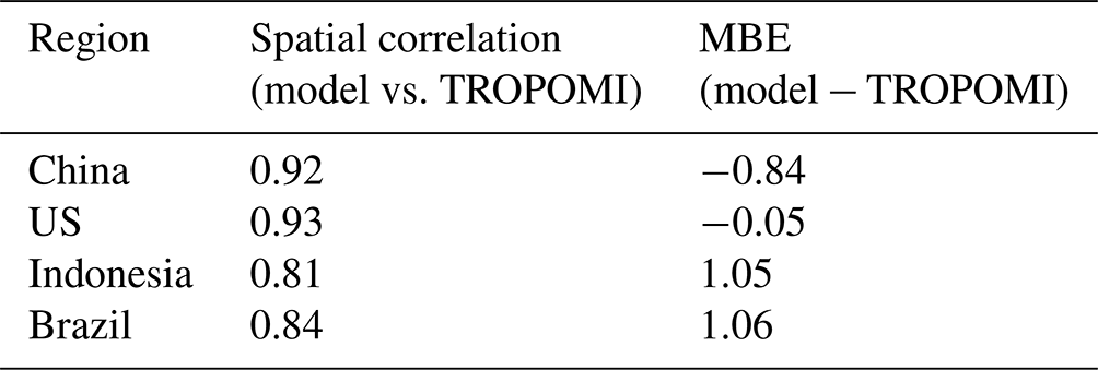
3.2 Comparisons for countries with large forested areas
Figure 3 shows the observed and simulated HCHO columns over countries where large forested areas are located. The definition of these countries used in the work of Opacka et al. (2021) was adopted. The statistics presented in Table 4 include regions with high and low biogenic activities. This section compares the overall biogenic emissions in the defined regions with literature values and assesses their impact on model performance.
Over China, CHASER correlates strongly with TROPOMI (r=0.92), with an MBE of −3 × 10¹⁵ molec. cm−2. The lowest differences between the datasets are observed primarily in the southeastern and western parts of China. The megacities of Shanghai, Nanjing, and Guangzhou are located in southeastern China. Consequently, CHASER has demonstrated good skills in the areas encompassed by multiple megacities. The annual isoprene emission for China from CHASER is 34 Tg C yr−1, which is higher than that found by Opacka et al. (2021) (9.5–23 Tg C yr−1).
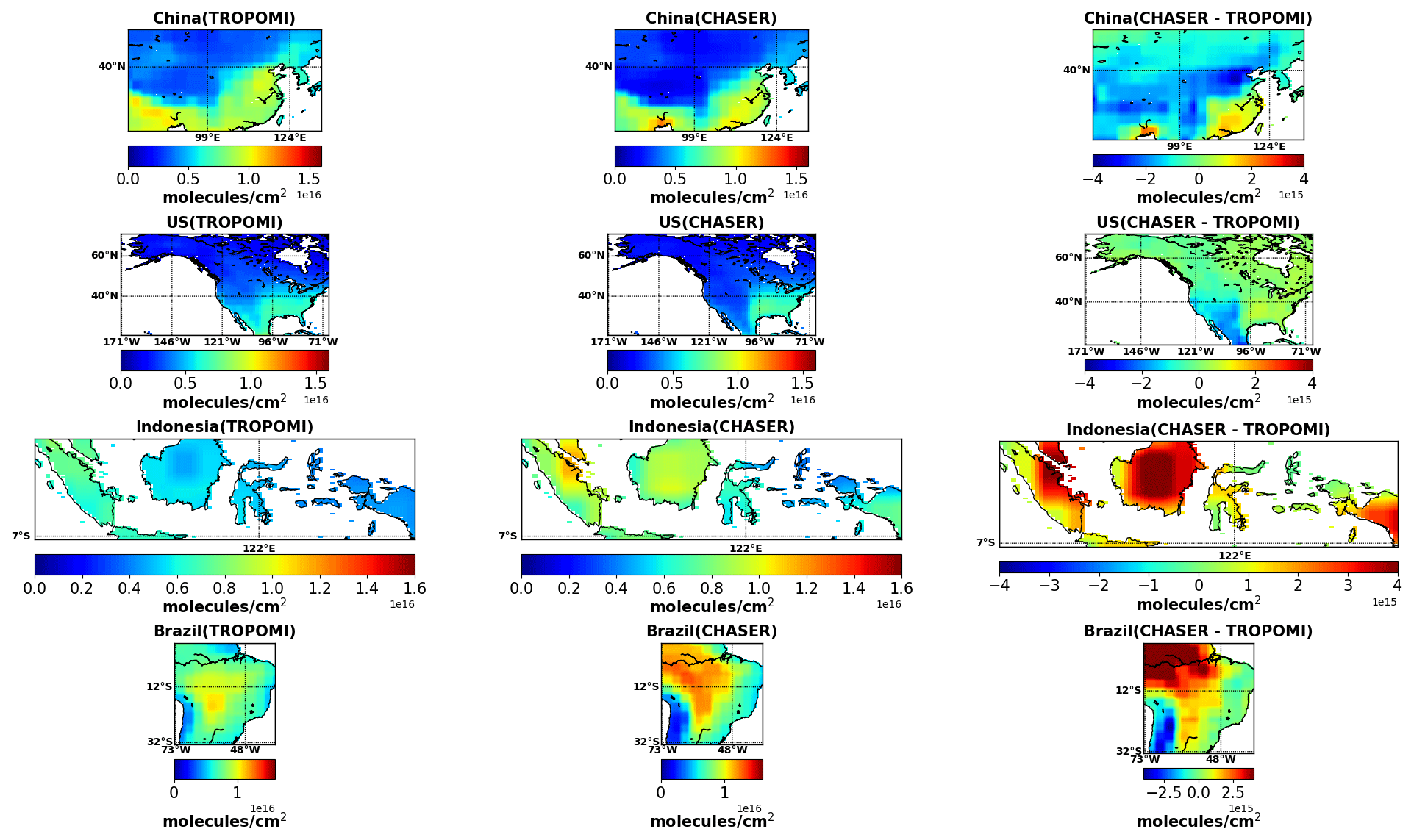
Figure 3Two-year (2019 and 2020) mean CHASER (first column) and TROPOMI (second column) HCHO columns (×1016 molec. cm−2 cm−2) in China (18.19–53.45° N, 73.67–135.02° E), the United States (18.91–45° N, 66–171° W), Indonesia (10° S–6° N, 95–142° E), and Brazil (33° S–5.24° N, 34–73° W). The differences between the datasets are presented in the third column. Only the coincident dates among the datasets are used to calculate the annual mean data.
Table 4Comparison of the 2-year mean HCHO (×1015 molec. cm−2) columns from TROPOMI and CHASER over countries with large forested areas. The coordinate bounds of the regions are adapted from Opacka et al. (2020). “Correlation” signifies the spatial agreement between CHASER and TROPOMI calculated from the annual mean data. The unit of MBE is ×1015 molec. cm−2.
CHASER has shown excellent skill in reproducing TROPOMI observations over the US. Along with high r values, the simulated magnitudes of the HCHO columns are consistent with observations throughout the whole region. Consequently, the bias between the datasets for the US is 2 %. In CHASER, annual isoprene emissions in the US and the southeastern US are 22 and 7.8 Tg C yr−1, respectively. Such values are within the ranges reported by Stavrakou et al. (2015) and Opacka et al. (2021).
The MBE between TROPOMI and CHASER in Indonesia is 1.05 × 10¹⁵ molec. cm−2. The r value is 0.81. Indonesia's annual mean TROPOMI and CHASER HCHO abundances are 5.06 × 10¹⁵ and 6.15 × 10¹⁵ molec. cm−2, respectively. The most significant differences between the datasets (4 × 10¹⁵ molec. cm−2) are observed for the islands of Sumatra, Borneo, and Sulawesi. Annual isoprene emissions in Indonesia used in the CHASER simulations are 42 Tg C yr−1. Indonesian isoprene emissions vary between 25.5 and 32 Tg C yr−1, depending on the land-use change (Opacka et al., 2021). Top-down estimates based on OMI and GOME-2 observations are ∼ 11 Tg C yr−1 (Stavrakou et al., 2015). However, the value of 11 Tg C yr−1 is half of the top-down estimate based on SCIAMACHY observations. Consequently, isoprene emissions in Indonesia remain very uncertain. However, CHASER estimates using VISIT emissions are higher than those reported in the literature, likely leading to overestimation by the model for Indonesia.
CHASER overestimates the HCHO columns over Amazonia (mostly in northern Brazil). Figure S6 shows the observed and simulated seasonal HCHO variation over Brazil. Although the model reproduced the temporal variability well, the magnitude was overestimated. This indicates that emission uncertainties are more prominent than uncertainties related to the chemical mechanism for this region. In CHASER, annual isoprene emissions over Amazonia are 67 Tg yr−1, consistent with the OMI-based top-down estimate of 70 Tg yr−1 obtained using a priori emissions from MEGAN (Stavrakou et al., 2015). However, deforestation affects the VOC emissions in the Amazon (Yáñez-Serrano et al., 2020). Massive deforestation occurred in the Amazon between 1985 and 2020, changing 11 % of the Amazonian biome (Cabarello et al., 2022). Depending on the land use and land cover change (LULCC), isoprene emissions in Brazil can vary between 79 and 106.5 Tg yr−1 (Opacka et al., 2021). Moreover, although biogenic VOC modeling for the Amazon has improved, VOC dynamics in the changing Amazonian biome are poorly understood (Salazar et al., 2018; Taylor et al., 2018). Therefore, updated biogenic VOC and LULCC inventories can potentially improve the model performance for Brazil.
In addition, CHASER isoprene emission estimates for Europe and Russia are, respectively, 17 and 15 Tg C yr−1, which are comparable to values reported in the literature (e.g., Guenther et al., 2006; Sinderolova et al., 2022).
This discussion focuses on isoprene emissions because isoprene is the dominant biogenic VOC (BVOC). Although not included in the current discussion, the chemical yield of HCHO from the oxidation of other BVOCs might also be a source of model uncertainty.
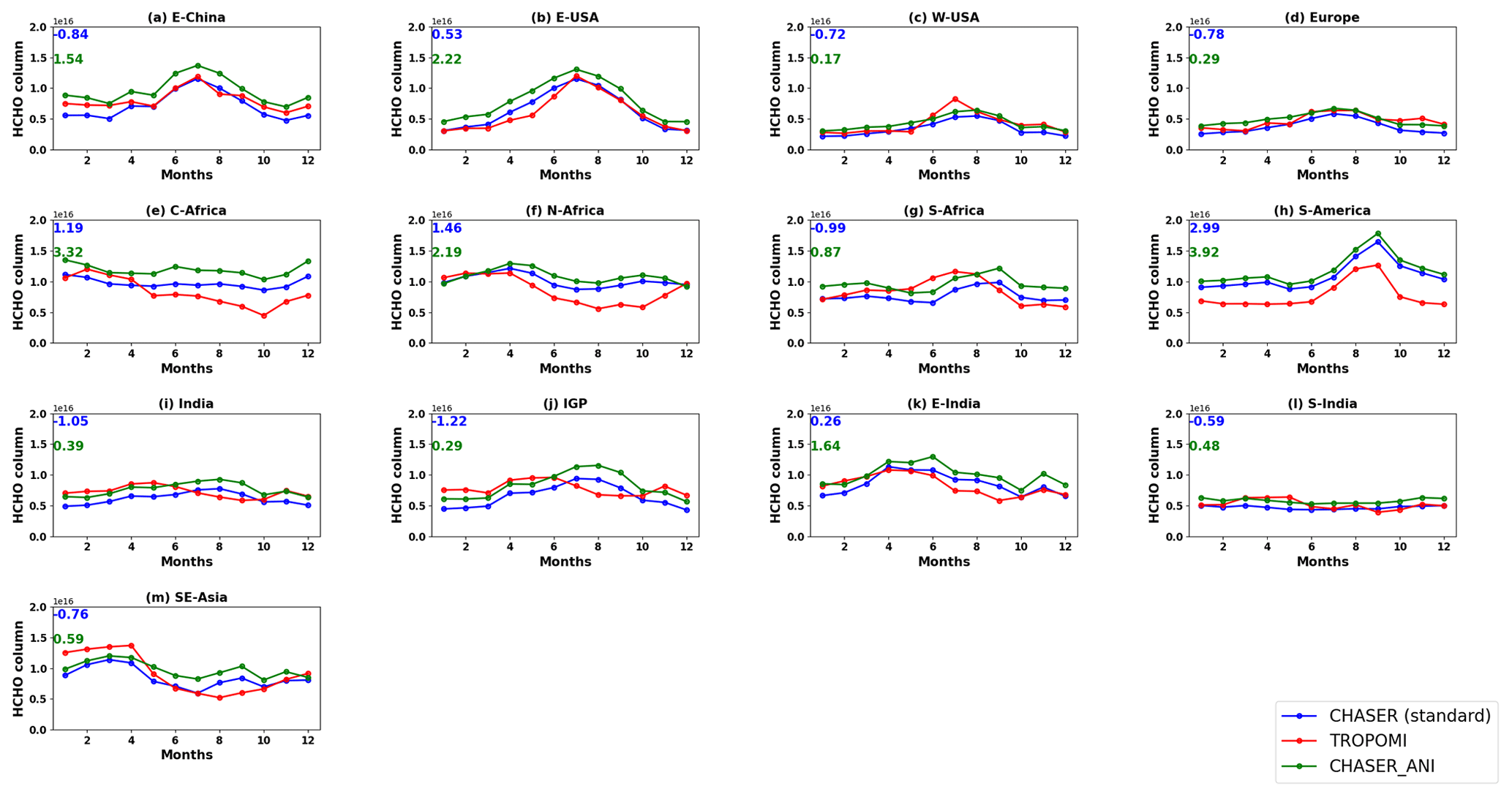
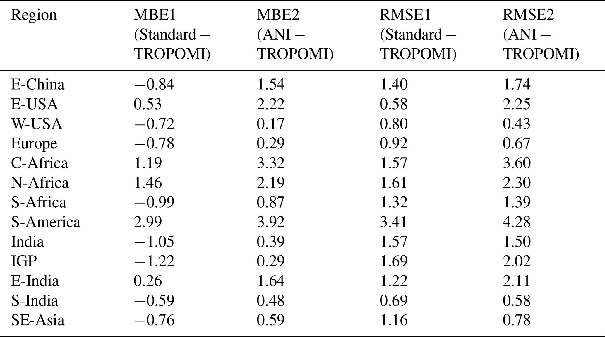
Figure 4Seasonal variation of HCHO (× 1016 molec. cm−2) in selected regions, as inferred from standard simulations (blue), TROPOMI observations (red), and ANI estimates (green). Anthropogenic VOC emissions are increased 3-fold in the ANI simulations. The blue numbers denote the MBE between the TROPOMI and CHASER HCHO columns. The MBE between the ANI and TROPOMI columns is shown in green. The coordinate bounds of the regions are similar to those used in Fig. 2. Simulations and observations in 2019 were used to calculate the monthly mean values.
3.3 Uncertainties related to anthropogenic VOC emissions
Uncertainties in anthropogenic VOC emissions can also be crucially important. Sensitivity simulations are performed by perturbing the anthropogenic VOC emissions. Perturbation effects are relevant when the anthropogenic VOC emissions are increased by 3-fold or more. We select the lowest perturbed simulation (i.e., a 3-fold increase; hereafter ANI). The better agreement between ANI and TROPOMI HCHO columns is attributed to underestimated anthropogenic VOC emissions in the standard simulation. Figure 4 compares the TROPOMI HCHO columns and ANI simulations for 2019. Standard simulation estimates for 2019 are also shown. The comparison statistics are provided in Table 5.
Over E-China (Fig. 4a) and India (Fig. 4i), ANI shows better agreement with TROPOMI than the standard simulation during winter. In India and China, the contribution of anthropogenic emissions to the NMVOC levels is more significant during the winter (Kumar et al., 2021; Liu et al., 2021). Thus, the ANI simulations improve the contribution of the wintertime anthropogenic VOCs in these regions. The ANI MBE and RMSE values over E-China are higher than those of the standard simulation. This indicates that the anthropogenic VOC estimates in E-China during the other seasons are reasonable. In contrast, the ANI simulations reduce the MBE values in India, indicating a greater underestimation of anthropogenic VOC emissions in this region than in E-China.
Similar to E-China, the ANI MBE and RMSE values are higher in C-Africa, N-Africa, S-Africa, South America, and E-USA. Over Europe (Fig. 4d) and W-USA (Fig. 4c), ANI RMSE values are lower than those of the standard simulation. The ANI simulations replicated the observed HCHO column magnitudes in both regions from October to December, resulting in lower RMSE values.
ANI estimates during the dry season in SE Asia (Fig. 4m) are similar to the standard simulation values, indicating a small effect of anthropogenic-emission uncertainties. The dry-season columns are overestimated when the anthropogenic VOC emissions are increased 5-fold (Fig. S7). Space-based observations have provided substantial evidence of increasing anthropogenic VOC emissions in Asian cities (Bauwens et al., 2022). Therefore, the anthropogenic-VOC-emission inventory should be updated to reduce the discrepancy between CHASER and TROPOMI over SE-Asia.
Table 5Comparison of regional mean tropospheric HCHO (× 1016 molec. cm−2) columns inferred from TROPOMI observations, the standard simulation, and ANI estimates. The units of MBE1, MBE2, RMSE1, and RMSE2 are ×1015 molec. cm−2. The simulations and observations for 2019 were used to calculate the statistics.
3.4 Impacts of NOx emission uncertainties on HCHO simulations
Uncertainties in the NOx emissions can affect the HCHO abundances through the NOx–HOx–VOC cycle. Such effects are assessed by comparing simulations that use different NOx inventories with the TROPOMI observations. The CHASER standard, OLNE, and TROPOMI HCHO columns are depicted in Fig. 5. The HTAP_v3 NOx emission inventory was replaced with the HTAP_v2.2 inventory in the OLNE simulations without altering the remaining emission inventories. The differences between the two NOx inventories are that (1) the HTAP_v3 inventory considers the changes in NOx emissions from 2000 to 2018, whereas the temporal coverage of HTAP_v2.2 is from 2008 to 2010, and (2) the emissions in HTAP_v3 have higher sectoral disaggregation (Crippa et al., 2023). The comparison-related statistics are given in Table S3. NOx emissions from both inventories are shown in Fig. S8.
On a global scale, HCHO column estimates are mostly unaffected by the changes in the NOx emission inventories, as indicated by the MBE values (Table 6). However, the RMSE is 8 % lower in the case of the standard simulation. OLNE estimates for higher latitudes (> = 50° N) are 5 % lower than those from the standard simulations. Such differences do not affect the model–satellite agreement in these regions.
The standard HCHO columns in India, China, and Southeast Asia are approximately 10 %–20 % lower than the OLNE estimates (Fig. 5c). In fact, those differences are consistent with changes in the regional OH estimates (Fig. 5d). This finding implies that the changes in the NOx emission estimates have affected the OH and HCHO abundances in these regions. Satellite data assimilation results reported by Miyazaki et al. (2017, 2020) indicate that NOx emissions in India have increased by 30 % since 2008, whereas NOx emissions in China have declined since 2011 (Liu et al., 2016). Over E-China (Fig. 5a and b), the standard simulations reduce the absolute annual mean difference between OLNE and TROPOMI of 3 × 10¹⁵ to 1 × 10¹⁵ molec. cm−2, which is consistent with the lower NOx emissions in this region in the updated inventory (Fig. S8). Over India and SE-Asia, the standard OH concentrations are ∼ 40 % lower (Fig. 5d) than the OLNE estimates, resulting in lower HCHO columns. The lower standard HCHO columns can be linked to the increasing NOx emissions in these regions (Fig. S8); however, the magnitude of the change in the NOx emissions for these regions in the updated inventory is likely overestimated.
In E-USA and W-USA (Table S3), the standard simulation reduces the MBE by 26 % and 12 %, respectively. The reductions in MBE and RMSE values in Africa and South America are less than 10 %. Therefore, NOx emission uncertainties mainly affect the HCHO simulations in India and SE Asia.
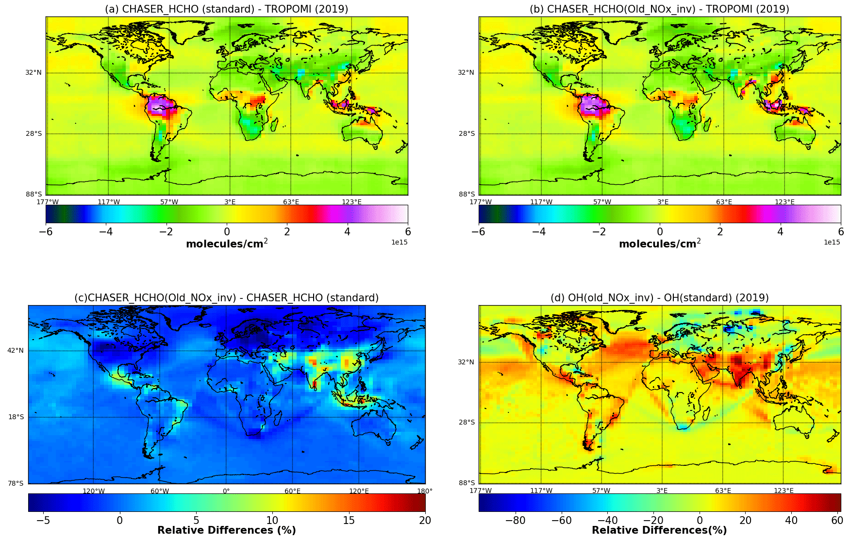
Figure 5Annual mean HCHO columns (×1016 molec. cm−2) in 2019, obtained from the (a) standard and (b) OLNE simulations. The HTAP-2008 NOx emission inventory was used instead of the HTAP-2018 inventory for the OLNE simulations (Table 1). The remaining emission inventories were similar in both simulations. (c) Global relative differences between the two HCHO simulations (OLNE−Standard). (d) Relative differences (global) between two OH (OLNE−Standard) simulations. The standard and OLNE OH simulation settings are similar to those described for Table 1. The OH and HCHO simulations were obtained simultaneously.
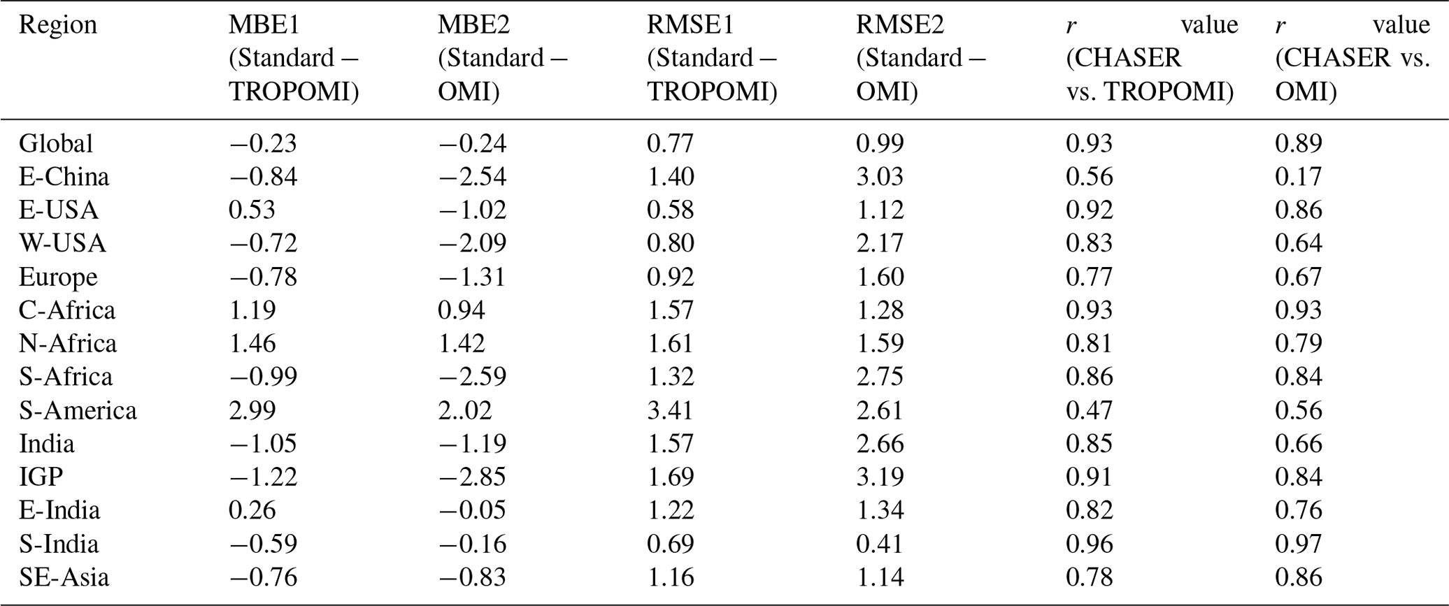
3.5 Comparison with OMI HCHO observations
TROPOMI was able to achieve improved precision of HCHO columns for shorter timescales (De Smedt et al., 2021). The effect of such a feature on the comparison results is evaluated in this section. The method of De Smedt et al. (2021) has been adopted to minimize the effect of the use of different cloud retrieval algorithms for OMI and TROPOMI retrievals. Figure S9 shows the global distribution of the mean HCHO columns obtained from TROPOMI and OMI retrievals and CHASER simulations in 2019 during the TROPOMI overpass time (13:30 LT). Only the coincident dates among the three datasets are shown. Global and regional comparison statistics are presented in Table 6.
The spatial correlation between OMI and CHASER is 0.89 (Table 6). OMI retrievals are positively biased by 7 % compared to CHASER results. A similar bias is also observed between TROPOMI and CHASER. Despite their similar MBE values, TROPOMI reduces the global RMSE by 20 %. Monthly MBE and RMSE values between OMI and CHASER are higher than those of TROPOMI and exhibit no seasonality (Table S3). The highest absolute differences between the model and OMI retrievals are observed in Amazonia in Brazil, C-Africa, and SE-Asia (Fig. S9). The magnitudes of the differences between the model and observations in these regions are similar for both sensors. Despite the improved resolution, TROPOMI and OMI show equivalent biases in regions with high HCHO levels (De Smedt et al., 2021). A regional comparison among the three datasets is portrayed in Fig. 6. The red (TROPOMI−CHASER) and green (OMI−CHASER) numbers are the respective MBE values.
Table 6Comparison of global and regional mean HCHO columns between satellite observations (TROPOMI and OMI) and standard CHASER simulations. The units of MBE and RMSE are × 1016 molec. cm−2. The r value signifies the spatial correlation. The statistics are based on simulations and observations for 2019.
Over E-China (Fig. 6a), the monthly mean TROPOMI columns are ∼ 22 % lower than those of OMI, which reduces the RMSE by 53 %. The simulated spatial distribution shows better congruence with the new observations. TROPOMI improved the summer model–satellite agreement considerably. The magnitude of the seasonal modulation in the three datasets is 50 %. Both sensors show that winter HCHO levels in E-China are ∼ 8 × 10¹⁵ molec. cm−2. Over E-USA (Fig. 6b), the r value between CHASER and OMI is 0.86. CHASER columns are underestimated compared to OMI, with MBE and RMSE values of and 1.1 × 10¹⁵ molec. cm−2, respectively. TROPOMI reduced the model–satellite RMSE by 50 % and improved the r value by 6 %. The most significant improvements were observed during the summer and autumn.
Over W-USA (Fig. 6c), TROPOMI retrievals are 26 % lower than OMI observations, which reduces the model–satellite RMSE by 63 %. The spatial correlation between OMI and CHASER is moderate. The simulated and TROPOMI wintertime columns are ∼ 30 % lower than OMI. However, the observed peak in HCHO seasonality in July is consistent with the observational datasets.
OMI and TROPOMI HCHO observations over Europe (Fig. 6d) are consistent. The seasonal cycle amplitude inferred from both sensors is 60 %. The simulated spatial distribution shows better agreement with the TROPOMI observations, demonstrating the effects of improved resolution.
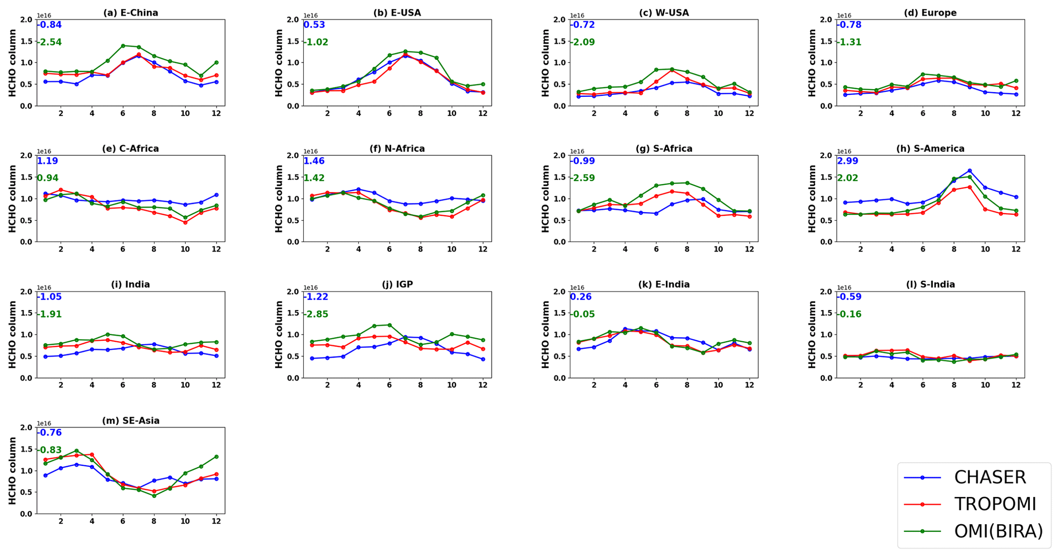
Figure 6Seasonal variation in HCHO (×1016 molec. cm−2) inferred from TROPOMI (red curve) and OMI (orange curve) retrievals and standard CHASER (blue curves) simulations. The region definitions are shown in Fig. S2. The blue numbers signify the MBE between TROPOMI and CHASER, whereas the green numbers represent the MBE between CHASER and OMI. Coincident dates in 2019 among the datasets are used to calculate the monthly mean data.
Over C-Africa (Fig. 6e), the RMSE value between CHASER and OMI is ∼ 18 % lower than that of TROPOMI. TROPOMI's values are biased by 18 % on the low side compared to OMI.
Over N-Africa (Fig. 6f), OMI retrievals are moderately correlated with CHASER. The amplitudes of seasonal modulation inferred from CHASER, TROPOMI, and OMI are 48 %, 62 %, and 66 %, respectively. The RMSE and MBE between OMI and CHASER are 1.41 × 10¹⁵ and 1.59 × 10¹⁵ molec. cm−2, respectively. OMI retrievals are approximately 13 % higher than TROPOMI retrievals. Simulated North African HCHO columns show better consistency with the observations during the biomass burning season.
Over S-Africa (Fig. 6g), OMI HCHO columns are biased by 32 % and 25 % on the high side compared to TROPOMI and CHASER. The simulated seasonal variabilities and spatial distribution of HCHO show more relevance to TROPOMI than to OMI.
Over S-America (Fig. 6h), the simulated peak (1.6 × 10¹⁶ molec. cm−2) in the HCHO seasonality shows strong congruence with the OMI observations. Despite such consistency, simulated values are higher than OMI retrievals, with MBE and RMSE values of ∼ 2 × 10¹⁵ molec. cm−2. Observations and simulations show that the peak HCHO abundances can vary between 1.0 × 10¹⁶–1.8 × 10¹⁶ molec. cm−2 in September. Although the r value between OMI and CHASER is higher than that of TROPOMI, the model's capability to replicate the observed spatial distribution was limited. OMI HCHO columns are positively biased by 30 % compared to TROPOMI, thereby reducing the model–satellite RMSE by 23 %.
Over India (Fig. 6i), CHASER HCHO columns are negatively biased by 23 % compared to OMI observations. Although TROPOMI minimized the model–satellite bias, seasonal discrepancies between the model and observations prevail. Over the IGP region, OMI HCHO retrievals are biased by 24 % and 36 % on the high side, respectively, compared to TROPOMI and CHASER. Both sensors captured similar HCHO seasonality in the IGP, with a modulation of 49 %. Although CHASER could not reproduce the seasonality, the simulated modulation is 48 %. The bias between the model and observations (OMI and TROPOMI) is ∼ 4 % in E-India and S-India. The simulated HCHO spatial variation strongly correlates with the observation datasets (r value of ∼ 0.85). The amplitude of the seasonal modulation in E-India inferred from OMI is ∼ 40 %.
Over Southeast Asia (Fig. 6m), CHASER columns are negatively biased by 19 % compared to the OMI columns. Despite lower biases, both datasets have similar model–satellite discrepancies during the dry season. A few reasons for the underestimation by CHASER in SE Asia during the dry season have been discussed in Sect. 3.2. In addition, assumptions used and uncertainties in the retrieval could also potentially engender this model–satellite discrepancy. Figure S10 compares CHASER and OMI SOA (González Abad et al., 2016) products. The data selection criterion is similar to the description presented in Sect. 2. The most relevant differences between the OMI BIRA and SAO products are related to the underlying CTMs that simulate the a priori profiles and the reference sector correction (Zhu et al., 2016). A comprehensive list of the differences between the two products is available from Zhu et al. (2016). The comparison statistics are given in Table S5. CHASER columns during the dry seasons in SE-Asia show excellent agreement with the OMI SOA retrievals (Fig. S10m). OMI SOA values during the dry season are negatively biased by 7 % compared to TROPOMI observations. The MBE between CHASER and the SOA product is 0.04 × 10¹⁵ molec. cm−2. Based on the comparison with OMI SOA products, the model performance during the dry season can be considered excellent. The emission estimates for SE-Asia in CHASER can be regarded as reasonable, too.
Similarly, in E-China (Fig. S10a), the OMI SOA product reduces the bias between the model and observations by 11 %. The simulated wintertime columns are consistent with the SOA estimates but underestimated compared to TROPOMI. The ANI estimates (Fig. 4a) for this region are higher than the SOA product, indicating that the anthropogenic emissions in CHASER for this region are rational. Therefore, uncertainties related to the retrieval procedure can also significantly affect the comparison results on a regional scale.
A comparison between CHASER and OMI BIRA HCHO products shows differences from the results of Hoque et al. (2022), where the simulation and observations for 2017 were used. The simulations in both studies are similar. However, the OMI data in the earlier study are systematically higher, which is the main cause of the statistically significant differences between the study results. A detailed investigation of the reasons will be addressed in a separate work.
3.6 Validation using MAX-DOAS observations
3.6.1 Seasonal variation
CHASER columns are compared with ground-based MAX-DOAS observations in Phimai, Chiba, and Kasuga in Fig. 7. Coincident TROPOMI observations over the sites are used for comparative discussion. The standard and OLNE simulations are used. MAX-DOAS observations between 12:00 and 15:00 LT were averaged to estimate the monthly mean columns. Only dates common to the three datasets were compared. De Smedt et al. (2021) compared the TROPOMI and A-SKY MAX-DOAS datasets in Phimai and Chiba. Because the comparison between the model and ground-based observations is the primary focus of this comparison effort, we do not consider the differences in the vertical sensitivities of TROPOMI and MAX-DOAS. Thus, the statistics will differ from those in De Smedt et al. (2021).
In Phimai, the standard CHASER HCHO seasonality correlates strongly (R=0.71) with the MAX-DOAS observations; it is underestimated by 39 %. However, the bias between the standard model estimates and TROPOMI observations is 4 %. Despite a strong correlation, TROPOMI observations are negatively biased by 37 % compared to MAX-DOAS (R=0.84). Such underestimation might be related to the coarse binning of the satellite data. Upon using finer binning, De Smedt et al. (2021) reported a negative bias of 23 % in Phimai.
Enhancements driven by biomass burning during the dry season (January–April) are well reflected in the simulations. During the wet season, MAX-DOAS, TROPOMI, and standard CHASER HCHO columns are mostly lower than 1 × 10¹⁶ molec. cm−2. The simulated standard HCHO peak in March is consistent with the satellite observations, whereas the MAX-DOAS observations show a peak during February. During the dry seasons of 2015 and 2016, the HCHO peak was observed in March (e.g., Hoque et al., 2018a). Consequently, such a shift in the HCHO peak might be related to fire numbers and fire radiative power changes (Hoque et al., 2022).
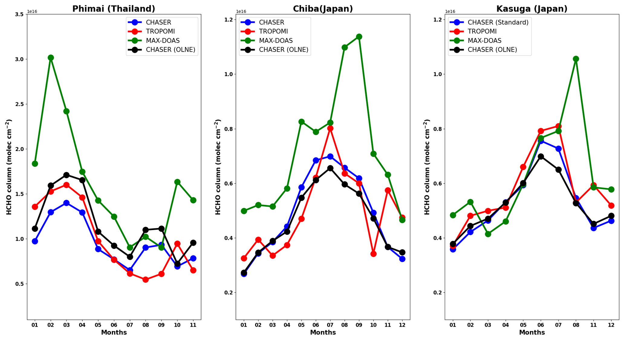
Figure 7Seasonal variations of HCHO (× 1016 molec. cm−2) columns inferred from satellite retrievals (red), model simulations (blue and black), and ground-based MAX-DOAS observations (green) in Phimai (Thailand), Chiba (Japan), and Kasuga (Japan). MAX-DOAS observations and CHASER simulations during 12:00–15:00 LT were selected for comparison. Dates common to the datasets are used to calculate the monthly mean statistics. The blue and black curves, respectively, signify the standard and OLNE simulations. TROPOMI AKs have been applied to both simulations. The simulation settings are provided in Table 1.
The bias between OLNE and MAX-DOAS observations is 27 %. OLNE estimates agree better with the TROPOMI observations during the dry season. However, the overall bias (13 %) between the model and satellite observations is higher in the case of OLNE simulations.
At Chiba, the simulated HCHO seasonality correlates strongly with the MAX-DOAS retrievals (R=0.81) and is negatively biased by ∼ 31 %. The amplitudes of seasonality inferred from the simulations, MAX-DOAS observations, and TROPOMI retrievals are, respectively, 59 %, 60 %, and 34 %. The MAX-DOAS, TROPOMI, and CHASER HCHO columns, respectively, reach their peaks in September, July, and June. Similar to Phimai, the HCHO peaks in satellite and ground-based observations differ. One reason might be the differences in spatial representativity. The TROPOMI data used for comparison are spatially averaged over 200 km centered on the Chiba site, whereas the spatial representativity of the MAX-DOAS is approx. 10 km. Moreover, MAX-DOAS observations are most sensitive to altitudes near the surface, whereas satellite sensitivity decreases near the surface. Consequently, the air masses sampled by the instruments at the same local time might differ, leading to inconsistent observation peaks.
At Kasuga, the simulated HCHO levels are strongly correlated with the TROPOMI observations (R=0.75) and are negatively biased by 35 %. Although the correlation between the model and MAX-DOAS retrievals is moderate, the bias between CHASER and MAX-DOAS retrievals is 14 %. Therefore, CHASER shows better agreement with MAX-DOAS than with TROPOMI. MAX-DOAS observations exhibit seasonality similar to that at Chiba, with the peak HCHO column occurring during August. Similar to Chiba, the satellite-observed and CHASER peaks are observed during July and June, respectively. The Chiba and Kasuga sites are located near the ocean and exhibit similar HCHO variability, which has been captured well in the simulations.
Although the bias between OLNE and standard simulations for Chiba and Kasuga is ∼ 4 %, the absolute difference is ∼ 1×10¹⁵ molec. cm−2. NOx emissions in Japan have not changed markedly since 2005 (Miyazaki et al., 2017). Differences between the simulations are observed during the summer, when isoprene emissions are expected to peak (Hoque et al., 2018a). Because the OH estimates over Japan are similar for both simulations (Fig. 5d), the differences are likely related to the interaction between the isoprene and NOx inventories.
3.6.2 Diurnal and daily variations
Figure 8 compares the observed and simulated daily and diurnal variations in the surface HCHO vmr. The error bars represent the 1σ standard deviation of the observed mean values. The daily variation comparison entails only the standard simulations.
In Phimai, the daily datasets correlate well, with an R value of 0.67. The slope of the fitted line is 0.35. The observed and simulated daily mean HCHO vmr is ∼ 4 ppbv. CHASER daily mean values are negatively biased by 19 % and 11 %, respectively, during the dry and wet seasons. The standard diurnal variations at Phimai are also well correlated with the observations (R=0.64). The simulated values lie within the standard deviation of the observations. HCHO mixing ratios show a peak (∼ 6 ppbv) at 08:00 LT in both datasets. The noontime (12:00 LT) vmr is approximately 4 ppbv, and hourly HCHO levels vary between 2 and 6 ppbv. The OLNE diurnal values are 20 % higher than the standard values. However, the mean absolute difference between the two simulations is 1 ppbv.
The standard simulation reproduced the observed diurnal variations at Chiba with a temporal correlation of 0.79, higher than at Phimai. Both simulations are biased by 10 % on the low side compared to the observations. No distinctive peak is observed in the diurnal variations. The increasing daytime HCHO levels in Chiba are well reflected in the model runs. The simulated daily mean values in Chiba are negatively biased by 18 %, with a temporal correlation of 0.40. The slope of the line fitted to the daily mean concentrations is 0.27, which is lower than at Phimai, suggesting greater underestimation, similar to the total columns (Fig. 7).
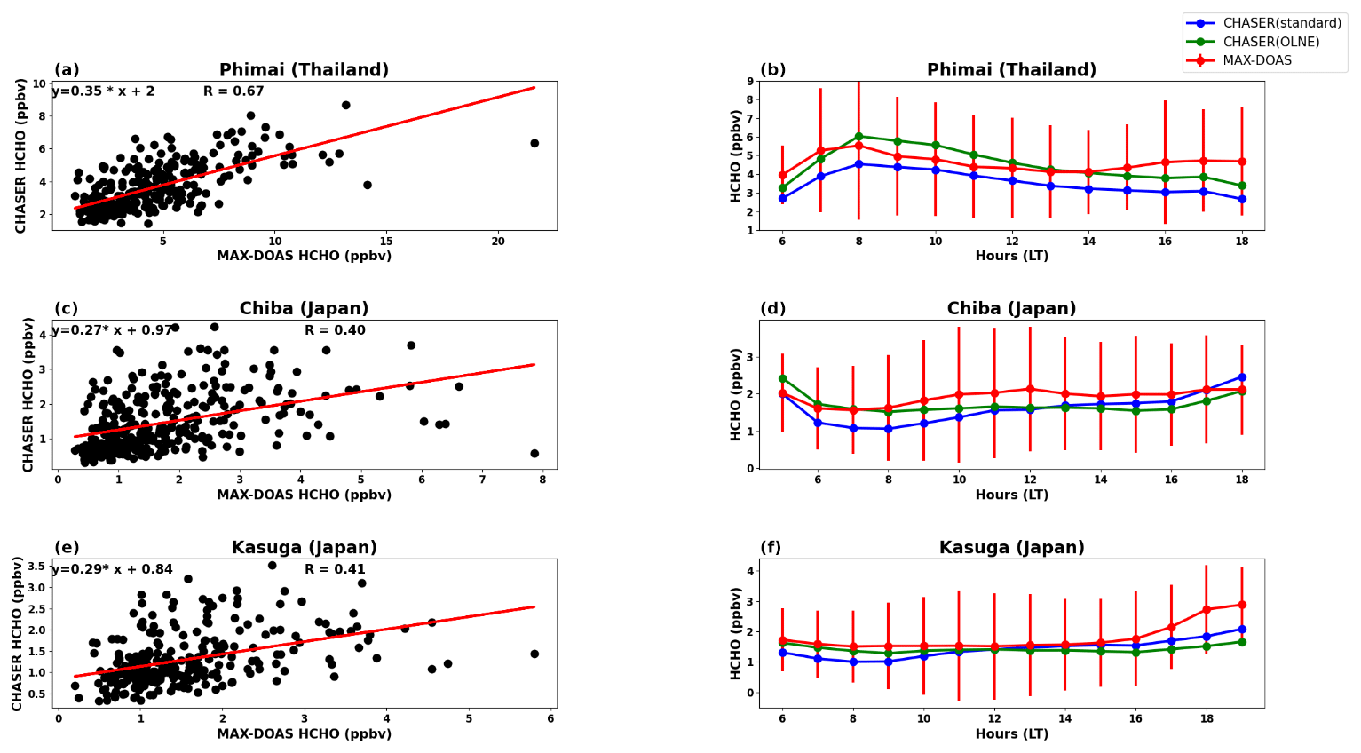
Figure 8(a, c, e) Scatter plots showing the correlation between the daily mean observed (MAX-DOAS) and simulated HCHO surface mixing ratios at the three sites. The standard simulations are used in the scatter plots. The linear fitted lines are shown in red. (b, d, f) Diurnal variations in the HCHO mixing ratios at the three sites are inferred from the MAX-DOAS observations and standard (blue) and OLNE (green) simulations. The error bars represent the 1σ standard deviation of the mean values estimated from the observations. Observations and simulations at coincident dates and times (local) are selected for comparison.
In Kasuga, modeled daily variations correlate moderately (R=0.41) with the observations. The effect of the NOx inventories on the simulated diurnal variations in Kasuga is not significant. The simulated daily mean values are negatively biased by 20 %, and the slope of the fit is 0.29. Although Chiba and Kasuga are similar sites, their observed diurnal variations are slightly different. However, the simulated values in both cases agree with the observed standard deviation.
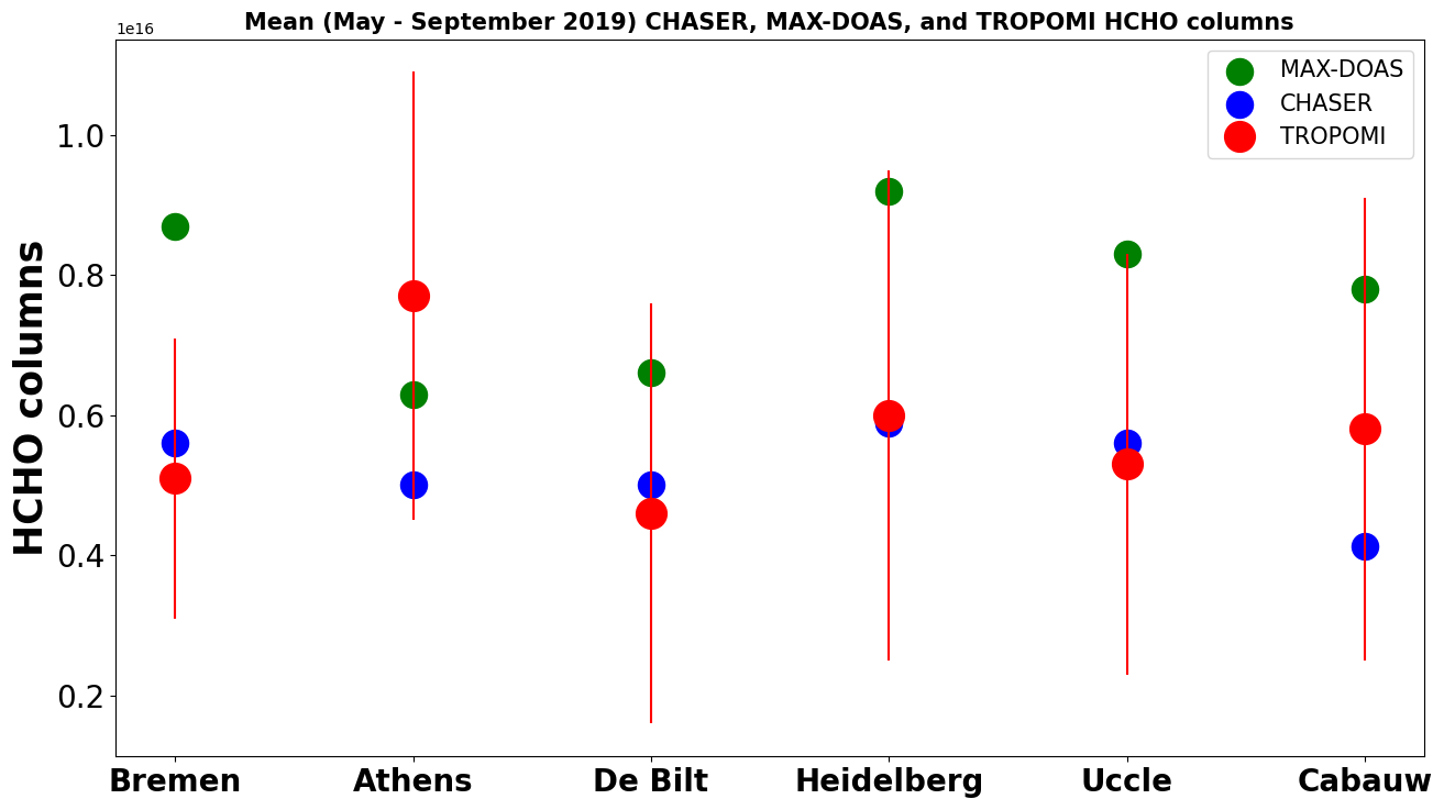
Figure 9Scatter plot comparing CHASER (red), MAX-DOAS (green), and TROPOMI (red) HCHO columns (× 1016 molec. cm−2) at a few European sites. The MAX-DOAS observed values are taken from the work of Oomen et al. (2024). These values represent the mean HCHO column from May to September in 2019. Observations made from 12:00–15:00 LT were used to calculate the mean values. Using a similar temporal filter, the modeled mean values were calculated from the simulations for 2019. TROPOMI data for 2019 were filtered as described in Sect. 2.2. The error bars signify the 1σ standard deviation of the TROPOMI mean HCHO columns.
In addition, CHASER HCHO columns are also compared with MAX-DOAS observations reported in the literature in Fig. 9. The observed values are obtained from Oomen et al. (2024). The observed mean values represent the averages of MAX-DOAS observations made between 12:00 and 15:00 LT from May to September 2019. A similar temporal filter was applied to the CHASER simulations for 2019. The coincident TROPOMI HCHO columns are also plotted. TROPOMI AKs are applied to the CHASER values. The error bars signify the 1σ standard deviation of the TROPOMI mean values.
Like the Asian sites, CHASER underestimates the HCHO columns at the European sites. All three datasets mostly agree within the 1σ variability range of the satellite observations. The CHASER and TROPOMI HCHO columns are lower than the MAX-DOAS observations except in Athens. CHASER shows better agreement with the MAX-DOAS observations in Athens. De Smedt et al. (2021) reported the biases between TROPOMI and MAX-DOAS observations at these sites, estimated from a daily timescale. As the simulated HCHO magnitude is consistent with the TROPOMI values, biases between the CHASER and MAX-DOAS HCHO columns at these sites will likely be equivalent.
3.7 Comparison with ATom-4 flight observations
Comparisons between simulated and observed HCHO and isoprene profiles along the ATom-4 flight path (Fig. S2) are depicted in Fig. 10a and c. Only the coincident dates have been included in the comparison.
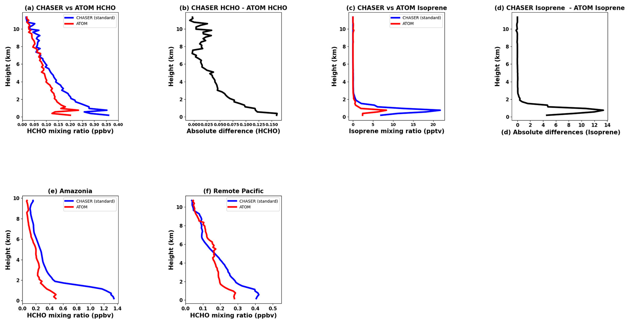
Figure 10The top panel shows comparisons between ATom-observed (red) and CHASER-simulated (blue) HCHO (a) and isoprene (c) profiles along the ATom-4 flight path in 2018. The ATom-4 flight path is depicted in Fig. S2. Standard simulations are used for comparison. Simulations for the times of the ATom observations were selected. Both datasets were averaged using 0.3 km bins. The relative differences between the observed and simulated (c) HCHO and (d) isoprene profiles are also shown. In the bottom panel, Atom-4-observed and CHASER-simulated HCHO profiles over (e) Amazonia and (f) the remote Pacific region are compared. Amazonia (10–40° W, 10° S–10° N) represents a densely vegetated region, whereas the remote Pacific region (160–180° W, 20° S–20° N) represents the background HCHO conditions. The units of the HCHO and isoprene mixing ratios are, respectively, parts per billion by volume (ppbv) and parts per trillion by volume (pptv).
The simulated HCHO and isoprene profiles agree well with the observations, with an R value of 0.95. Above and below 4 km, CHASER HCHO profiles are positively biased by 29 % and 62 %, respectively, compared to ATom-4 HCHO levels. The absolute difference in the isoprene profiles around 1 km is 14 pptv, which strongly correlates with the difference in the HCHO profile below 2 km. This finding signifies that overestimated CHASER isoprene mixing ratios induce a positive bias in the HCHO estimates. Despite non-significant isoprene mixing ratios at altitudes greater than 2 km, both datasets show considerable HCHO levels above 2 km. Zhao et al. (2022) reported a similar finding and attributed the HCHO mixing ratios above 2 km to enhanced CH4 oxidation. At higher altitudes, HCHO is produced through the CH3O2 (methyl peroxy radical) + CH3O2 pathway initiated by CH4 oxidation (i.e., CH4 + OH). HCHO production through this pathway is considered in CHASER. Therefore, despite the differences in magnitude, CHASER has shown good skills in reproducing the VOC profiles.
The potential reason for the higher simulated HCHO values below 2 km could be CHASER's overestimation of the HCHO mixing ratios over South America, mainly the Amazon (Fig. 2c). Figure 10e and f depict the observed and simulated HCHO profiles over the Amazon (10–40° W, 10° S–10° N) and the remote Pacific region (160–180° W, 20° S–20° N), respectively. The HCHO profiles over the remote Pacific region represent the background HCHO mixing ratio. The CHASER and ATom background HCHO mixing ratios within the boundary layer are 0.4 and 0.3 ppbv, respectively. The mean relative differences between the two datasets within the boundary layer over Amazonia and the remote Pacific region are ∼ 60 % and ∼ 22 %, respectively, indicating that the uncertainty in the contributions from the isoprene emissions to the total HCHO uncertainties is higher. Above 5 km, CHASER underestimates the background HCHO mixing ratios. However, the simulated and TROPOMI HCHO columns over the remote Pacific region showed consistency when gridded over the same horizontal grid (Fig. 1). Consequently, differences in the horizontal resolution can cause discrepancies between the simulations and ATom observations over the remote region. Over South America, the model overestimates the observed (TROPOMI and ATom) HCHO abundances, irrespective of the horizontal resolution. Therefore, the biogenic emission estimates for South America in CHASER should be reviewed to reduce the model–observation biases.
3.8 Contribution estimates
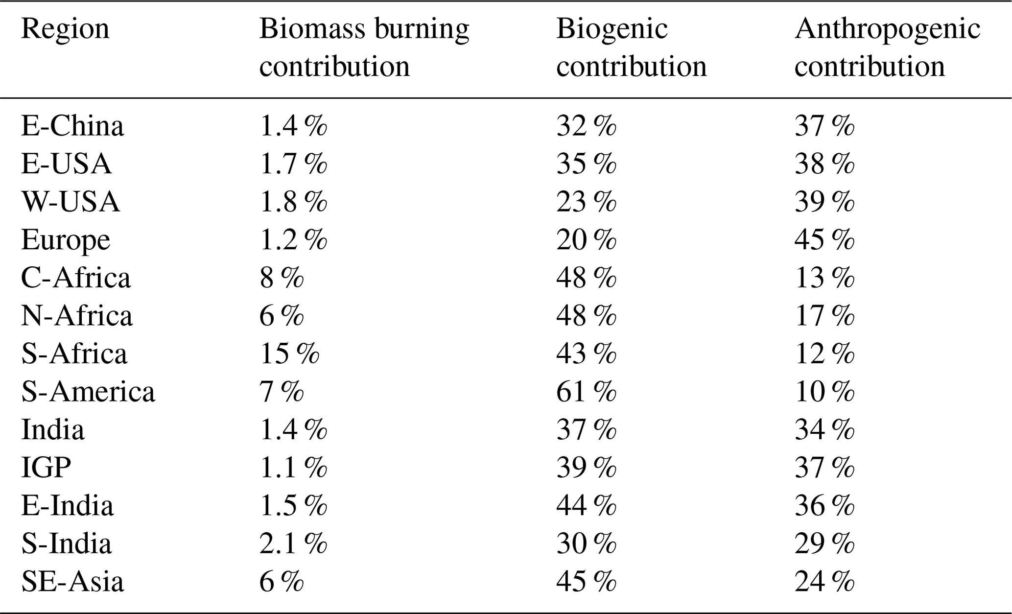
The contributions of different VOC emission sources to the regional HCHO abundances are presented in Fig. 11. The contribution estimates are presented in Table 8. A stacked-bar plot of the annual contributions of the emission sources is portrayed in Fig. S11.
Over E-China (Fig. 11a), biomass burning has a non-significant effect on the regional HCHO columns. During summer, the biogenic and anthropogenic VOC emission contributions are 44 % and 17 %, respectively. In contrast, the anthropogenic and biogenic contributions to the regional HCHO level during winter are 35 % and 13 %, respectively.
Non-significant biomass burning effects on the HCHO columns can be observed over E-USA (Fig. 11b), W-USA (Fig. 11c), and Europe (Fig. 11d). Biogenic emissions contribute more than 20 % (35 % in E-USA) in these regions. In these regions, the annual anthropogenic contributions are higher than the biogenic contribution. Although the simulated winter columns in these regions are consistent with TROPOMI (Fig. 2), the model values are lower during summer and autumn. Moreover, the sensitivity results show a non-significant biogenic contribution during winter and autumn, which likely reduces the annual biogenic contribution estimates.
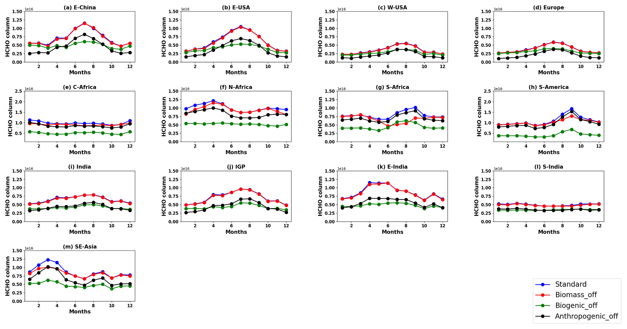
Figure 11Seasonal variation of HCHO (× 1016 molec. cm−2) inferred from different simulations. The settings of the standard simulation are presented in Table 1. The model estimates shown in red, green, and blue are simulated by switching off the biomass burning, biogenic, and anthropogenic emissions. The satellite AKs have been applied to all the simulations. The coordinate bounds of the regions are similar to those in Fig. 2.
In C-Africa (Fig. 11e), biogenic emissions (48 %) are the most significant contributor, followed by anthropogenic emissions (13 %). Although the biogenic emission contributions in N-Africa (Fig. 11f; 48 %) and S-Africa (Fig. 11b; 43 %) are equivalent, the pyrogenic contributions are twice as high in the latter region. Consequently, despite similar HCHO abundances and modulations in these regions, the source contributions differ.
Table 7Contributions (%) of different emission sources to HCHO abundances in selected regions. The respective emissions were switched off to estimate the contribution to the total HCHO abundances. The contributions have been calculated with respect to the standard simulations. The satellite AKs were applied to all simulations.
Biogenic emissions over South America (Fig. 11h) contribute 61 % of the regional HCHO abundances. The pyrogenic contribution during the biomass burning period is 12 %, whereas the annual contribution is 7 %.
In SE-Asia (Fig. 11m), the annual anthropogenic contributions are ∼ 20 %. During the dry season, the anthropogenic, pyrogenic, and biogenic contributions are 7 %, 12 %, and 48 %, respectively. Biogenic production comprises 43 % of the HCHO columns from July to December, whereas anthropogenic emissions account for 9 %.
In India (Fig. 11i), annual pyrogenic emissions contribute ∼ 2 % of the HCHO levels. A similar source contribution to the HCHO levels in the IGP (Fig. 11j) is also observed. The model's capability to reproduce the observed HCHO seasonality in India and the IGP region was limited. Consequently, robust source contribution estimates for these regions cannot be derived from the current analysis.
Over E-India (Fig. 11k), 44 % of the HCHO levels originate from biogenic sources, followed by anthropogenic VOC emissions (36 %). Similar source contributions of biogenic (30 %) and anthropogenic (29 %) emissions are observed in S-India (Fig. 11l). Over both regions, the pyrogenic source contribution is ∼ 2 %.
3.9 Uncertainties in the chemical mechanism
Uncertainties in the chemical mechanisms affect the HCHO simulations. The representation of isoprene chemistry can vary among the gas-phase chemistry mechanisms used in the CTMs. The most commonly used isoprene schemes underestimate the observed HCHO by at least 15 % (Marvin et al., 2017). Such underestimations are also strongly linked with the errors in the NOx emission inventories (Anderson et al., 2017). In addition, potential errors in the acetaldehyde emissions and chemistry can also lead to the underestimation of the HCHO vmr by up to 75 pptv in the lower troposphere (Anderson et al., 2017).
CHASER-simulated global HCHO spatiotemporal distributions at a horizontal resolution of 2.8° × 2.8° were evaluated against multi-platform observations. First, 2 years of simulation results (2019–2020) were compared with the latest HCHO satellite observations from TROPOMI. The model–satellite agreement was excellent, with a global r value of 0.93 and an RMSE of 0.75 × 10¹⁵ molec. cm−2. The model showed a good capability to reproduce the HCHO columns in hotspot and background regions. CHASER HCHO columns over large forested areas showed good consistency with the observations, demonstrating that the biogenic emission estimates in the model are reasonable. The simulated HCHO seasonality in a few selected regions was consistent with the observations. The model was able to reproduce the observed wintertime HCHO columns in E-USA, W-USA, and Europe, in addition to summer peaks. Disagreement between TROPOMI and CHASER was observed primarily in India, China, Amazonia, and SE-Asia. Uncertainties in background HCHO columns, anthropogenic-VOC-emission inventories, the chemical mechanisms adopted in the model, and retrieval algorithms were the potential contributors to these discrepancies. However, those uncertainties did not affect the model–satellite agreement in Africa and South America. A comparison between OMI, TROPOMI, and CHASER HCHO columns demonstrated that the effect of TROPOMI's improved spatial resolution was limited globally. However, in most regions, the simulated HCHO seasonality showed better agreement with TROPOMI than with OMI, reducing the RMSE by up to 63 %. TROPOMI retrievals were, on average, 30 % lower than those of OMI.
Second, CHASER simulations were compared with 2 years of MAX-DOAS observations of HCHO at Phimai, Chiba, and Kasuga. Daily CHASER HCHO mixing ratios showed consistency with the observations at the three sites, with R values of 0.39–0.67. The slopes from linear fitting were lower for Chiba (0.29) and Kasuga (0.29) than for Phimai (0.37), implying that there is less underestimation by the model for the latter site. The diurnal variations at the sites were consistent with the observations. Changing the NOx emission inventories did not affect the simulated diurnal variations.
Third, simulated HCHO and isoprene profiles for 2018 were compared with ATom-4 flight observations. Despite consistent profile shapes, the model overestimated VOC mixing ratios (mainly within the PBL). Uncertainties related to VOC emission inventories, background HCHO levels, and the model resolution were potential reasons for the model–flight discrepancies.
Lastly, sensitivity studies were conducted to estimate the contributions of the different emissions sources to the total HCHO columns in different regions. Biogenic emissions were the most significant contributor in most of the regions. In a few cases, biogenic and anthropogenic emission contributions were equivalent. In some regions, only summertime biogenic estimates were found to be reasonable.
The CHASER source code needed to reproduce the simulations in this work is available from the repository at https://doi.org/10.5281/zenodo.10892945 (Sudo, 2024).
The processed model output and observational datasets needed to reproduce the results are available from the repository at https://doi.org/10.5281/zenodo.10052384 (Hoque et al., 2024). The MAX-DOAS profile and column data provided by Hitoshi Irie can be accessed from the repository (i.e., Hoque et al., 2024). TROPOMI (https://scihub.copernicus.eu/dhus/#/home, last access: 1 July 2023; De Smedt et al., 2021), OMI-BIRA-product (https://www.temis.nl/qa4ecv/hcho/hcho_omi.php, last access: 1 July 2023; De Smedt et al., 2021), and ATom (https://daac.ornl.gov/ATOM/guides/ATom_nav.html, last access: 1 July 2023; https://doi.org/10.3334/ORNLDAAC/1581, Wofsy et al., 2018) data were obtained from the respective websites.
HMSH conceptualized the study, conducted the model simulations, analyzed the datasets, and drafted the manuscript. YH helped with the data processing. HI developed the JM2 code and maintained the A-SKY network. KS developed the CHASER model and supervised the study. MFK used his expertise to explain the results. All the authors commented and provided feedback on the final results and manuscript.
The contact author has declared that none of the authors has any competing interests.
Publisher’s note: Copernicus Publications remains neutral with regard to jurisdictional claims made in the text, published maps, institutional affiliations, or any other geographical representation in this paper. While Copernicus Publications makes every effort to include appropriate place names, the final responsibility lies with the authors.
We are grateful to the TROPOMI, OMI, and ATom scientific teams for making the respective observational datasets available for public usage. The CHASER model simulations were partly performed with the supercomputer (NEC SX-Aurora TSUBASA) at the National Institute for Environmental Studies (NIES), Tsukuba, Japan. The corresponding author acknowledges the valuable advice of Kazuyakai Miyazaki (Jet Propulsion Lab., NASA) and Takashi Sekiya (JAMSTEC, Japan).
This research has been supported by the Ministry of the Environment, Government of Japan (grant nos. Global Research Fund S-12 and Global Research Fund S-20), the Japan Society for the Promotion of Science (grant nos. JP20H04320, JP19H05669, JP19HO4235, JP23H04971, JP21K12227, JP22H03727, and JP22H05004), the Environmental Restoration and Conservation Agency (grant no. JPMEERF20215005), and the Japan Aerospace Exploration Agency (grant no. 19RT000351).
This paper was edited by Jason Williams and reviewed by Narendra Ojha and three anonymous referees.
Anderson, D. C., Nicely, J. M., Wolfe, G. M., Hanisco, T. F., Salawitch, R. J., Canty, T. P.,Dickerson, R. R., Apel, E. C., Baidar, S., Bannan, T. J., Blake, N. J., Chen, D., Dix, B., Fernandez, R. P., Hall, S. R., Hornbrook, R. S., Huey, L. G., Josse, B., Jockel, P., Kinnison, D. E., Koenig, T. K., Le Breton, M., Marecal, V., Morgenstern, O., Oman, L. D., Pan, L. L., Percival, C., Plummer, D., Revell, L. E., Rozanov, E., Saiz-Lopez, A., Stenke, A., Sudo, K.,Tilmes, S., Ullman, K., Volkamer, R., Weinheimer, A. J., and Zeng, G.: Formaldehyde in the tropical western Pacific: Chemical sources and sinks, convective transport, and representation in CAM-Chem and the CCMI models, J. Geophys. Res., 122, 201–211, https://doi.org/10.1002/2016JD026121, 2017.
Apel, E. C., Asher, E. C., Hills, A. J., and Hornbrook, R. S.: ATom: Volatile Organic Compounds (VOCs) from the TOGA instrument, Version 2, ORNL DAAC [data set], Oak Ridge, Tennessee, USA, https://doi.org/10.3334/ORNLDAAC/1936, 2021.
Arlander, D., Brüning, D., Schmidt, U., and Ehhalt, D.: The tropospheric distribution of formaldehyde during TROPOZ II, J. Atmos. Chem., 22, 251–269, https://doi.org/10.1007/BF00696637, 1995.
Bauwens, M., Verreyken, B., Stavrakou, T., Müller, J., and De Smedt, I.: Spaceborne evidence for significant anthropogenic VOC trends in Asian cities over 2005–2019, Environ. Res. Lett., 17, 015008, https://doi.org/10.1088/1748-9326/ac46eb/, 2022.
Boersma, K. F., Eskes, H. J., and Brinksma, E. J. : Error analysis for tropospheric NO2 retrieval from space. J. Geophys. Res., 109, D04311, https://doi.org/10.1029/2003JD003962, 2004.
Boersma, K. F., Vinken, G. C. M., and Eskes, H. J.: Representativeness errors in comparing chemistry transport and chemistry climate models with satellite UV–Vis tropospheric column retrievals, Geosci. Model Dev., 9, 875–898, https://doi.org/10.5194/gmd-9-875-2016, 2016.
Burkert, J., Andrés-Hernández, M. D., Stöbener, D., Burrows, J. P., Weissenmayer, M., and Kraus, A.: Peroxy radical and related trace gas measurements in the boundary layer above the Atlantic Ocean, J. Geophys. Res., 106, 5457–5477, https://doi.org/10.1029/2000JD900613, 2001.
Burrows, J. P., Weber, M., Buchwitz, M., Rozanov, V., Ladstätter-Weißenmayer, A., Richter, A., DeBeek, R., Hoogen, R., Bramstedt, K., Eichmann, K.-U., Eisinger, M., and Perner, D.: The Global Ozone Monitoring Experiment (GOME): Mission Concept and First Scientific Results, J. Atmos. Sci., 56, 151–175, https://doi.org/10.1175/1520-0469(1999)056<0151:TGOMEG>2.0.CO;2, 1999.
Caballero, C. B., Ruhoff, A., and Biggs, T.: Land use and land cover changes and their impacts on surface-atmosphere interactions in Brazil: A systematic review, Sci. Total Environ., 808, 152134, https://doi.org/10.1016/j.scitotenv.2021.152134, 2022.
Cazorla, M., Wolfe, G. M., Bailey, S. A., Swanson, A. K., Arkinson, H. L., and Hanisco, T. F.: A new airborne laser-induced fluorescence instrument for in situ detection of formaldehyde throughout the troposphere and lower stratosphere, Atmos. Meas. Tech., 8, 541–552, https://doi.org/10.5194/amt-8-541-2015, 2015.
Chan, K. L., Wiegner, M., van Geffen, J., De Smedt, I., Alberti, C., Cheng, Z., Ye, S., and Wenig, M.: MAX-DOAS measurements of tropospheric NO2 and HCHO in Munich and the comparison to OMI and TROPOMI satellite observations, Atmos. Meas. Tech., 13, 4499–4520, https://doi.org/10.5194/amt-13-4499-2020, 2020.
Chutia, L., Ojha, N., Girach, I. A., Sahu, L. K., Alvarado, M. A. L., Burrows, J. P., Pathak, B., and Bhuyan, P. K.: Distribution of volatile organic compounds over Indian subcontinent during winter: WRF-chem simulation versus observations, Environ. Pol., 252, 256–269, https://doi.org/10.1016/j.envpol.2019.05.097, 2019.
Colella, P. and Woodward, P. R.: The piecewise parabolic method (PPM) for gas-dynamical simulations, J. Comput. Phys., 54, 174–201, https://doi.org/10.1016/0021-9991(84)90143-8, 1984.
Crippa, M., Guizzardi, D., Butler, T., Keating, T., Wu, R., Kaminski, J., Kuenen, J., Kurokawa, J., Chatani, S., Morikawa, T., Pouliot, G., Racine, J., Moran, M. D., Klimont, Z., Manseau, P. M., Mashayekhi, R., Henderson, B. H., Smith, S. J., Suchyta, H., Muntean, M., Solazzo, E., Banja, M., Schaaf, E., Pagani, F., Woo, J.-H., Kim, J., Monforti-Ferrario, F., Pisoni, E., Zhang, J., Niemi, D., Sassi, M., Ansari, T., and Foley, K.: The HTAP_v3 emission mosaic: merging regional and global monthly emissions (2000–2018) to support air quality modelling and policies, Earth Syst. Sci. Data, 15, 2667–2694, https://doi.org/10.5194/essd-15-2667-2023, 2023.
De Smedt, I., Müller, J.-F., Stavrakou, T., van der A, R., Eskes, H., and Van Roozendael, M.: Twelve years of global observations of formaldehyde in the troposphere using GOME and SCIAMACHY sensors, Atmos. Chem. Phys., 8, 4947–4963, https://doi.org/10.5194/acp-8-4947-2008, 2008.
De Smedt, I., Stavrakou, T., Müller, J.-F., van der A, R. J., and Van Roozendael, M.: Trend detection in satellite observations of formaldehyde tropospheric columns, Geophys. Res. Lett., 37, L18808, https://doi.org/10.1029/2010GL044245, 2010.
De Smedt, I., Stavrakou, T., Hendrick, F., Danckaert, T., Vlemmix, T., Pinardi, G., Theys, N., Lerot, C., Gielen, C., Vigouroux, C., Hermans, C., Fayt, C., Veefkind, P., Müller, J.-F., and Van Roozendael, M.: Diurnal, seasonal and long-term variations of global formaldehyde columns inferred from combined OMI and GOME-2 observations, Atmos. Chem. Phys., 15, 12519–12545, https://doi.org/10.5194/acp-15-12519-2015, 2015.
De Smedt, I., Yu, H., Richter, A., Beirle, S., Eskes, H., Boersma, K. F., Van Roozendael, M., Van Geffen, J., Lorente, A., and Peters, E.: QA4ECV HCHO tropospheric column data from OMI (Version 1.1), Royal Belgian Institute for Space Aeronomy [data set], https://doi.org/10.18758/71021031, 2017.
De Smedt, I., Theys, N., Yu, H., Danckaert, T., Lerot, C., Compernolle, S., Van Roozendael, M., Richter, A., Hilboll, A., Peters, E., Pedergnana, M., Loyola, D., Beirle, S., Wagner, T., Eskes, H., van Geffen, J., Boersma, K. F., and Veefkind, P.: Algorithm theoretical baseline for formaldehyde retrievals from S5P TROPOMI and from the QA4ECV project, Atmos. Meas. Tech., 11, 2395–2426, https://doi.org/10.5194/amt-11-2395-2018, 2018.
De Smedt, I., Pinardi, G., Vigouroux, C., Compernolle, S., Bais, A., Benavent, N., Boersma, F., Chan, K.-L., Donner, S., Eichmann, K.-U., Hedelt, P., Hendrick, F., Irie, H., Kumar, V., Lambert, J.-C., Langerock, B., Lerot, C., Liu, C., Loyola, D., Piters, A., Richter, A., Rivera Cárdenas, C., Romahn, F., Ryan, R. G., Sinha, V., Theys, N., Vlietinck, J., Wagner, T., Wang, T., Yu, H., and Van Roozendael, M.: Comparative assessment of TROPOMI and OMI formaldehyde observations and validation against MAX-DOAS network column measurements, Atmos. Chem. Phys., 21, 12561–12593, https://doi.org/10.5194/acp-21-12561-2021, 2021.
Duncan, B. N., Yoshida, Y., Olson, J. R., Sillman, S., Martin, R. V., Lamsal, L., Hu, Y., Pickering, K. E., Retscher, C., Allen, D. J., and Crawford, J. H.: Application of OMI observations to a space-based indicator of NOx and VOC controls on surface ozone formation, Atmos. Environ., 44, 2213–2223, https://doi.org/10.1016/j.atmosenv.2010.03.010, 2010.
Emori, S., Nozawa, T., Numaguti, A., and Uno, I.: Importance of cumulus parameterization for precipitation simulation over East Asia in June, J. Meteorol. Soc. Jpn., 79, 939–947, https://doi.org/10.2151/jmsj.79.939, 2021.
Franco, B., Hendrick, F., Van Roozendael, M., Müller, J.-F., Stavrakou, T., Marais, E. A., Bovy, B., Bader, W., Fayt, C., Hermans, C., Lejeune, B., Pinardi, G., Servais, C., and Mahieu, E.: Retrievals of formaldehyde from ground-based FTIR and MAX-DOAS observations at the Jungfraujoch station and comparisons with GEOS-Chem and IMAGES model simulations, Atmos. Meas. Tech., 8, 1733–1756, https://doi.org/10.5194/amt-8-1733-2015, 2015.
Fu, T. M., Jacob, D. J., Wittrock, F., Burrows, J. P., Vrekoussis, M., and Henze, D. K.: Global budgets of atmospheric glyoxal and methylglyoxal, and implications for formation of secondary organic aerosols, J. Geophys. Res., 113, D15303, https://doi.org/10.1029/2007JD009505, 2008.
González Abad, G., Vasilkov, A., Seftor, C., Liu, X., and Chance, K.: Smithsonian Astrophysical Observatory Ozone Mapping and Profiler Suite (SAO OMPS) formaldehyde retrieval, Atmos. Meas. Tech., 9, 2797–2812, https://doi.org/10.5194/amt-9-2797-2016, 2016.
Guenther, A.: Seasonal and spatial variations in natural volatile organic compound emissions, Ecol. Appl., 7, 34–45, https://doi.org/10.2307/2269405, 1997.
Guenther, A., Karl, T., Harley, P., Wiedinmyer, C., Palmer, P. I., and Geron, C.: Estimates of global terrestrial isoprene emissions using MEGAN (Model of Emissions of Gases and Aerosols from Nature), Atmos. Chem. Phys., 6, 3181–3210, https://doi.org/10.5194/acp-6-3181-2006, 2006.
Ha, P. T. M., Kanaya, Y., Taketani, F., Andrés Hernández, M. D., Schreiner, B., Pfeilsticker, K., and Sudo, K.: Implementation of HONO into the chemistry–climate model CHASER (V4.0): roles in tropospheric chemistry, Geosci. Model Dev., 16, 927–960, https://doi.org/10.5194/gmd-16-927-2023, 2023.
Hak, C., Pundt, I., Trick, S., Kern, C., Platt, U., Dommen, J., Ordóñez, C., Prévôt, A. S. H., Junkermann, W., Astorga-Lloréns, C., Larsen, B. R., Mellqvist, J., Strandberg, A., Yu, Y., Galle, B., Kleffmann, J., Lörzer, J. C., Braathen, G. O., and Volkamer, R.: Intercomparison of four different in-situ techniques for ambient formaldehyde measurements in urban air, Atmos. Chem. Phys., 5, 2881–2900, https://doi.org/10.5194/acp-5-2881-2005, 2005.
He, Y., Hoque, H. M. S., and Sudo, K.: Introducing new lightning schemes into the CHASER (MIROC) chemistry–climate model, Geosci. Model Dev., 15, 5627–5650, https://doi.org/10.5194/gmd-15-5627-2022, 2022.
Hoque, H. M. S., Irie, H., and Damiani, A.: First MAX-DOAS Observations of Formaldehyde and Glyoxal in Phimai, Thailand, J. Geophys. Res., 123, 9957–9975, https://doi.org/10.1029/2018JD028480, 2018a.
Hoque, H. M. S., Irie, H., Damiani, A., Rawat, P., and Naja, M.: First simultaneous observations of formaldehyde and glyoxal by MAX-DOAS in the Indo-Gangetic Plain region, Sola, 14, 159–164, https://doi.org/10.2151/sola.2018-028, 2018b.
Hoque, H. M. S., Sudo, K., Irie, H., Damiani, A., Naja, M., and Fatmi, A. M.: Multi-axis differential optical absorption spectroscopy (MAX-DOAS) observations of formaldehyde and nitrogen dioxide at three sites in Asia and comparison with the global chemistry transport model CHASER, Atmos. Chem. Phys., 22, 12559–12589, https://doi.org/10.5194/acp-22-12559-2022, 2022.
Hoque, H. M. S., Sudo, K., and Irie, H.: Model and observational datasets used for evaluating CHASER simulated formaldehyde (HCHO) abundances in 2019 and 2020, Zenodo [data set], https://doi.org/10.5281/zenodo.10052384, 2024.
Inness, A., Baier, F., Benedetti, A., Bouarar, I., Chabrillat, S., Clark, H., Clerbaux, C., Coheur, P., Engelen, R. J., Errera, Q., Flemming, J., George, M., Granier, C., Hadji-Lazaro, J., Huijnen, V., Hurtmans, D., Jones, L., Kaiser, J. W., Kapsomenakis, J., Lefever, K., Leitão, J., Razinger, M., Richter, A., Schultz, M. G., Simmons, A. J., Suttie, M., Stein, O., Thépaut, J.-N., Thouret, V., Vrekoussis, M., Zerefos, C., and the MACC team: The MACC reanalysis: an 8 yr data set of atmospheric composition, Atmos. Chem. Phys., 13, 4073–4109, https://doi.org/10.5194/acp-13-4073-2013, 2013.
Irie, H.: International air quality and sky research remote sensing network (A-SKY): Its development and satellite atmosphere product validation, J. Remote Sens. Soc. Jpn., 41, 575–581, https://doi.org/10.11440/rssj.41.575, 2021.
Irie, H., Kanaya, Y., Akimoto, H., Iwabuchi, H., Shimizu, A., and Aoki, K.: First retrieval of tropospheric aerosol profiles using MAX-DOAS and comparison with lidar and sky radiometer measurements, Atmos. Chem. Phys., 8, 341–350, https://doi.org/10.5194/acp-8-341-2008, 2008.
Irie, H., Takashima, H., Kanaya, Y., Boersma, K. F., Gast, L., Wittrock, F., Brunner, D., Zhou, Y., and Van Roozendael, M.: Eight-component retrievals from ground-based MAX-DOAS observations, Atmos. Meas. Tech., 4, 1027–1044, https://doi.org/10.5194/amt-4-1027-2011, 2011.
Irie, H., Nakayama, T., Shimizu, A., Yamazaki, A., Nagai, T., Uchiyama, A., Zaizen, Y., Kagamitani, S., and Matsumi, Y.: Evaluation of MAX-DOAS aerosol retrievals by coincident observations using CRDS, lidar, and sky radiometer in Tsukuba, Japan, Atmos. Meas. Tech., 8, 2775–2788, https://doi.org/10.5194/amt-8-2775-2015, 2015.
Ito, A. and Inatomi, M.: Use of a process-based model for assessing the methane budgets of global terrestrial ecosystems and evaluation of uncertainty, Biogeosciences, 9, 759–773, https://doi.org/10.5194/bg-9-759-2012, 2012.
Jenkin, M. E., Young, J. C., and Rickard, A. R.: The MCM v3.3.1 degradation scheme for isoprene, Atmos. Chem. Phys., 15, 11433–11459, https://doi.org/10.5194/acp-15-11433-2015, 2015.
Kaiser, J., Wolfe, G. M., Bohn, B., Broch, S., Fuchs, H., Ganzeveld, L. N., Gomm, S., Häseler, R., Hofzumahaus, A., Holland, F., Jäger, J., Li, X., Lohse, I., Lu, K., Prévôt, A. S. H., Rohrer, F., Wegener, R., Wolf, R., Mentel, T. F., Kiendler-Scharr, A., Wahner, A., and Keutsch, F. N.: Evidence for an unidentified non-photochemical ground-level source of formaldehyde in the Po Valley with potential implications for ozone production, Atmos. Chem. Phys., 15, 1289–1298, https://doi.org/10.5194/acp-15-1289-2015, 2015.
Khan, M. F., Latif, M. T., Saw, W. H., Amil, N., Nadzir, M. S. M., Sahani, M., Tahir, N. M., and Chung, J. X.: Fine particulate matter in the tropical environment: monsoonal effects, source apportionment, and health risk assessment, Atmos. Chem. Phys., 16, 597–617, https://doi.org/10.5194/acp-16-597-2016, 2016.
Kleipool, Q. L., Dobber, M. R., de Haan, J. F., and Levelt, P. F.: Earth surface reflectance climatology from 3 years of OMI data, J. Geophys. Res., 113, D18308, https://doi.org/10.1029/2008JD010290, 2008.
Kreher, K., Van Roozendael, M., Hendrick, F., Apituley, A., Dimitropoulou, E., Frieß, U., Richter, A., Wagner, T., Lampel, J., Abuhassan, N., Ang, L., Anguas, M., Bais, A., Benavent, N., Bösch, T., Bognar, K., Borovski, A., Bruchkouski, I., Cede, A., Chan, K. L., Donner, S., Drosoglou, T., Fayt, C., Finkenzeller, H., Garcia-Nieto, D., Gielen, C., Gómez-Martín, L., Hao, N., Henzing, B., Herman, J. R., Hermans, C., Hoque, S., Irie, H., Jin, J., Johnston, P., Khayyam Butt, J., Khokhar, F., Koenig, T. K., Kuhn, J., Kumar, V., Liu, C., Ma, J., Merlaud, A., Mishra, A. K., Müller, M., Navarro-Comas, M., Ostendorf, M., Pazmino, A., Peters, E., Pinardi, G., Pinharanda, M., Piters, A., Platt, U., Postylyakov, O., Prados-Roman, C., Puentedura, O., Querel, R., Saiz-Lopez, A., Schönhardt, A., Schreier, S. F., Seyler, A., Sinha, V., Spinei, E., Strong, K., Tack, F., Tian, X., Tiefengraber, M., Tirpitz, J.-L., van Gent, J., Volkamer, R., Vrekoussis, M., Wang, S., Wang, Z., Wenig, M., Wittrock, F., Xie, P. H., Xu, J., Yela, M., Zhang, C., and Zhao, X.: Intercomparison of NO2, O4, O3 and HCHO slant column measurements by MAX-DOAS and zenith-sky UV–visible spectrometers during CINDI-2, Atmos. Meas. Tech., 13, 2169–2208, https://doi.org/10.5194/amt-13-2169-2020, 2020.
Kumar, A., Hakkim, H., Ghude, S. D., and Sinha, V.: Probing wintertime air pollution sources in the Indo-Gangetic Plain through 52 hydrocarbons measured rarely at Delhi and Mohali, Sci. Total Environ., 801, 149711, https://doi.org/10.1016/j.scitotenv.2021.149711, 2021.
Kupc, A., Williamson, C., Wagner, N. L., Richardson, M., and Brock, C. A.: Modification, calibration, and performance of the Ultra-High Sensitivity Aerosol Spectrometer for particle size distribution and volatility measurements during the Atmospheric Tomography Mission (ATom) airborne campaign, Atmos. Meas. Tech., 11, 369–383, https://doi.org/10.5194/amt-11-369-2018, 2018.
Kurucz, R. L., Furenlid, I., Brault, J., and Testerman, L.: Solar flux atlas from 296 to 1300 nm, National Solar Observatory Atlas No. 1, Sunspot, New Mexico, 1984.
Kuttippurath, J., Abbhishek, K., Gopikrishnan, G. S., and Pathak, M.: Investigation of long–term trends and major sources of atmospheric HCHO over India, Environ. Chall., 7, 100477, https://doi.org/10.1016/j.envc.2022.100477, 2022.
Lee, M., Heikes, B. G., Jacob, D. J., Sachse, G., and Anderson, B.: Hydrogen peroxide, organic hydroperoxide, and formaldehyde as primary pollutants from biomass burning, J. Geophys. Res., 102, 1301–1309, https://doi.org/10.1029/96JD01709, 1997.
Levelt, P. F., Joiner, J., Tamminen, J., Veefkind, J. P., Bhartia, P. K., Stein Zweers, D. C., Duncan, B. N., Streets, D. G., Eskes, H., van der A, R., McLinden, C., Fioletov, V., Carn, S., de Laat, J., DeLand, M., Marchenko, S., McPeters, R., Ziemke, J., Fu, D., Liu, X., Pickering, K., Apituley, A., González Abad, G., Arola, A., Boersma, F., Chan Miller, C., Chance, K., de Graaf, M., Hakkarainen, J., Hassinen, S., Ialongo, I., Kleipool, Q., Krotkov, N., Li, C., Lamsal, L., Newman, P., Nowlan, C., Suleiman, R., Tilstra, L. G., Torres, O., Wang, H., and Wargan, K.: The Ozone Monitoring Instrument: overview of 14 years in space, Atmos. Chem. Phys., 18, 5699–5745, https://doi.org/10.5194/acp-18-5699-2018, 2018.
Levelt, P. F., Stein Zweers, D. C., Aben, I., Bauwens, M., Borsdorff, T., De Smedt, I., Eskes, H. J., Lerot, C., Loyola, D. G., Romahn, F., Stavrakou, T., Theys, N., Van Roozendael, M., Veefkind, J. P., and Verhoelst, T.: Air quality impacts of COVID-19 lockdown measures detected from space using high spatial resolution observations of multiple trace gases from Sentinel-5P/TROPOMI, Atmos. Chem. Phys., 22, 10319–10351, https://doi.org/10.5194/acp-22-10319-2022, 2022.
Liu, F., Zhang, Q., van der A, R. J., Zheng, B., Tong, D., Yan, L., Zheng, Y., and He, K.: Recent reduction in NOx emissions over China: synthesis of satellite observations and emission inventories, Environ. Res. Lett., 11, 114002, https://doi.org/10.1088/1748-9326/11/11/114002, 2016.
Liu, Y., Wang, H., Jing, S., Peng, Y., Gao, Y., Yan, R., Wang, Q., Lou, S., Cheng, T., and Huang, C.: Strong regional transport of volatile organic compounds (VOCs) during wintertime in Shanghai megacity of China, Atmos. Environ., 244, 117940, https://doi.org/10.1016/j.atmosenv.2020.117940, 2021.
Luecken, D. J., Napelenok, S. L., Strum, M., Scheffe, R., and Phillips, S.: Sensitivity of Ambient Atmospheric Formaldehyde and Ozone to Precursor Species and Source Types Across the United States, Environ. Sci. Technol., 52, 4668–4675, https://doi.org/10.1021/acs.est.7b05509, 2018.
Marvin, M. R., Wolfe, G. M., Salawitch, R. J., Canty, T. P., Roberts, S. J., Travis, K. R., Aikin, K. C., de Gouw, J. A., Graus, M., Hanisco, T. F., Holloway, J. S., Hübler, G., Kaiser, J., Keutsch, F. N., Peischl, J., Pollack, I. B., Roberts, J. M., Ryerson, T. B., Veres, P. R., and Warneke, C.: Impact of evolving isoprene mechanisms on simulated formaldehyde: An inter-comparison supported by in situ observations from SENEX, Atmos. Environ., 164, 325–336, https://doi.org/10.1016/j.atmosenv.2017.05.049, 2017.
Martin, R. V., Fiore, A. M., and Van Donkelaar, A.: Space-based diagnosis of surface ozone sensitivity to anthropogenic emissions, Geophys. Res. Lett., 31, L06120, https://doi.org/10.1029/2004GL019416, 2004.
Meller, R. and Moortgat, G. K.: Temperature dependence of the absorption cross section of HCHO between 223 and 323 K in the wavelength range 225–375 nm, J. Geophys. Res., 105, 7089–7102, https://doi.org/10.1029/1999JD901074, 2000.
Mellor, G. L. and Yamada, T.: A hierarchy of turbulence closure models for planetary boundary layers, J. Atmos. Sci., 31, 1791–1806, https://doi.org/10.1175/1520-0469(1974)031<1791:AHOTCM>2.0.CO;2, 1974.
Miyazaki, K., Eskes, H., Sudo, K., Boersma, K. F., Bowman, K., and Kanaya, Y.: Decadal changes in global surface NOx emissions from multi-constituent satellite data assimilation, Atmos. Chem. Phys., 17, 807–837, https://doi.org/10.5194/acp-17-807-2017, 2017.
Miyazaki, K., Bowman, K., Sekiya, T., Eskes, H., Boersma, F., Worden, H., Livesey, N., Payne, V. H., Sudo, K., Kanaya, Y., Takigawa, M., and Ogochi, K.: Updated tropospheric chemistry reanalysis and emission estimates, TCR-2, for 2005–2018, Earth Syst. Sci. Data, 12, 2223–2259, https://doi.org/10.5194/essd-12-2223-2020, 2020.
Müller, J.-F., Stavrakou, T., Wallens, S., De Smedt, I., Van Roozendael, M., Potosnak, M. J., Rinne, J., Munger, B., Goldstein, A., and Guenther, A. B.: Global isoprene emissions estimated using MEGAN, ECMWF analyses and a detailed canopy environment model, Atmos. Chem. Phys., 8, 1329–1341, https://doi.org/10.5194/acp-8-1329-2008, 2008.
Munro, R., Lang, R., Klaes, D., Poli, G., Retscher, C., Lindstrot, R., Huckle, R., Lacan, A., Grzegorski, M., Holdak, A., Kokhanovsky, A., Livschitz, J., and Eisinger, M.: The GOME-2 instrument on the Metop series of satellites: instrument design, calibration, and level 1 data processing – an overview, Atmos. Meas. Tech., 9, 1279–1301, https://doi.org/10.5194/amt-9-1279-2016, 2016.
Oomen, G.-M., Müller, J.-F., Stavrakou, T., De Smedt, I., Blumenstock, T., Kivi, R., Makarova, M., Palm, M., Röhling, A., Té, Y., Vigouroux, C., Friedrich, M. M., Frieß, U., Hendrick, F., Merlaud, A., Piters, A., Richter, A., Van Roozendael, M., and Wagner, T.: Weekly derived top-down volatile-organic-compound fluxes over Europe from TROPOMI HCHO data from 2018 to 2021, Atmos. Chem. Phys., 24, 449–474, https://doi.org/10.5194/acp-24-449-2024, 2024.
Opacka, B., Müller, J.-F., Stavrakou, T., Bauwens, M., Sindelarova, K., Markova, J., and Guenther, A. B.: Global and regional impacts of land cover changes on isoprene emissions derived from spaceborne data and the MEGAN model, Atmos. Chem. Phys., 21, 8413–8436, https://doi.org/10.5194/acp-21-8413-2021, 2021.
Possanzini, M., Palo, V. D., and Cecinato, A.: Sources and photodecomposition of formaldehyde and acetaldehyde in Rome ambient air, Atmos. Environ., 36, 3195–3201, https://doi.org/10.1016/S1352-2310(02)00192-9, 2002.
Price, C. and Rind, D. : A simple lightning parameterization for calculating global lightning distributions, J. Geophys. Res., 97, 9919–9933, https://doi.org/10.1029/92JD00719, 1992.
Roberts, G., Wooster, M. J., and Lagoudakis, E.: Annual and diurnal african biomass burning temporal dynamics, Biogeosciences, 6, 849–866, https://doi.org/10.5194/bg-6-849-2009, 2009.
Roscoe, H. K., Van Roozendael, M., Fayt, C., du Piesanie, A., Abuhassan, N., Adams, C., Akrami, M., Cede, A., Chong, J., Clémer, K., Friess, U., Gil Ojeda, M., Goutail, F., Graves, R., Griesfeller, A., Grossmann, K., Hemerijckx, G., Hendrick, F., Herman, J., Hermans, C., Irie, H., Johnston, P. V., Kanaya, Y., Kreher, K., Leigh, R., Merlaud, A., Mount, G. H., Navarro, M., Oetjen, H., Pazmino, A., Perez-Camacho, M., Peters, E., Pinardi, G., Puentedura, O., Richter, A., Schönhardt, A., Shaiganfar, R., Spinei, E., Strong, K., Takashima, H., Vlemmix, T., Vrekoussis, M., Wagner, T., Wittrock, F., Yela, M., Yilmaz, S., Boersma, F., Hains, J., Kroon, M., Piters, A., and Kim, Y. J.: Intercomparison of slant column measurements of NO2 and O4 by MAX-DOAS and zenith-sky UV and visible spectrometers, Atmos. Meas. Tech., 3, 1629–1646, https://doi.org/10.5194/amt-3-1629-2010, 2010.
Ryan, R. G., Silver, J. D., Querel, R., Smale, D., Rhodes, S., Tully, M., Jones, N., and Schofield, R.: Comparison of formaldehyde tropospheric columns in Australia and New Zealand using MAX-DOAS, FTIR and TROPOMI, Atmos. Meas. Tech., 13, 6501–6519, https://doi.org/10.5194/amt-13-6501-2020, 2020.
Salazar, D., Lokvam, J., Mesones, I., Vásquez Pilco, M., Ayarza Zuñiga, J. M., de Valpine, P., and Fine, P. V. A.: Origin and maintenance of chemical diversity in a species-rich tropical tree lineage, Nat. Ecol. Evol., 2, 983–990, https://doi.org/10.1038/s41559-018-0552-0, 2018.
Sekiya, T. and Sudo, K. : Roles of transport and chemistry processes in global ozone change on interannual and multidecadal time scales, J. Geophys. Res., 119, 4903–4921, https://doi.org/10.1002/2013JD020838, 2014.
Sekiya, T., Miyazaki, K., Ogochi, K., Sudo, K., and Takigawa, M.: Global high-resolution simulations of tropospheric nitrogen dioxide using CHASER V4.0, Geosci. Model Dev., 11, 959–988, https://doi.org/10.5194/gmd-11-959-2018, 2018.
Sekiya, T., Miyazaki, K., Eskes, H., Bowman, K., Sudo, K., Kanaya, Y., and Takigawa, M.: The worldwide COVID-19 lockdown impacts on global secondary inorganic aerosols and radiative budget, Sci. Adv., 9, eadh2688, https://doi.org/10.1126/sciadv.adh2688, 2023.
Simpson, I. J., Blake, D. R., Blake, N. J., Meinardi, S., Barletta, B., Hughes, S. C., Fleming, L. T., Crawford, J. H., Diskin, G. S., Emmons, L. K., Fried, A., Guo, H., Peterson, D. A., Wisthaler, A., Woo, J.-H., Barré, J., Gaubert, B., Kim, J., Kim, M. J., Kim, Y., Knote, C., Mikoviny, T., Pusede, S. E., Schroeder, J. R., Wang, Y., Wennberg, P. O., and Zeng, L.: Characterization, sources, and reactivity of volatile organic compounds (VOCs) in Seoul and surrounding regions during KORUS-AQ, Elementa, 8, 37, https://doi.org/10.1525/elementa.434, 2020.
Sindelarova, K., Markova, J., Simpson, D., Huszar, P., Karlicky, J., Darras, S., and Granier, C.: High-resolution biogenic global emission inventory for the time period 2000–2019 for air quality modelling, Earth Syst. Sci. Data, 14, 251–270, https://doi.org/10.5194/essd-14-251-2022, 2022.
Singh, H., Salas, L., Chatfield, R., Czech, E., Fried, A., Walega, J., Evans, M., Field, B., Jacob, D., and Blake, D.: Analysis of the atmospheric distribution, sources, and sinks of oxygenated volatile organic chemicals based on measurements over the Pacific during TRACE-P, J. Geophys. Res., 109, https://doi.org/10.1029/2003JD003883, 2004.
Sinreich, R., Frieß, U., Wagner, T., and Platt, U.: Multi-axis differential optical absorption spectroscopy (MAX-DOAS) of gas and aerosol distributions, Faraday Discuss., 130, 153–164, https://doi.org/10.1039/B419274P, 2005.
Souri, A. H., Chance, K., Bak, J., Nowlan, C. R., González Abad, G., Jung, Y., Wong, D. C., Mao, J., and Liu, X.: Unraveling pathways of elevated ozone induced by the 2020 lockdown in Europe by an observationally constrained regional model using TROPOMI, Atmos. Chem. Phys., 21, 18227–18245, https://doi.org/10.5194/acp-21-18227-2021, 2021.
Spurr, R. J. D.: LIDORT and VLIDORT: Linearized pseudo-spherical scalar and vector discrete ordinate radiative transfer models for use in remote sensing retrieval problems, Light Scattering Reviews, edited by: Kokhanovsky, A., Berlin, Springer, 229–271, https://doi.org/10.1007/978-3-540-48546-9_7, 2008.
Stavrakou, T., Müller, J.-F., Bauwens, M., De Smedt, I., Van Roozendael, M., De Mazière, M., Vigouroux, C., Hendrick, F., George, M., Clerbaux, C., Coheur, P.-F., and Guenther, A.: How consistent are top-down hydrocarbon emissions based on formaldehyde observations from GOME-2 and OMI?, Atmos. Chem. Phys., 15, 11861–11884, https://doi.org/10.5194/acp-15-11861-2015, 2015.
Stewart, G. J., Nelson, B. S., Acton, W. J. F., Vaughan, A. R.. Hopkins, J. R., Yunus, S. S. M., Hewitt, C. N., Wild, O., Nemitz, E., Gadi, R., Sahu, L. K., Mandal, T. K., Gurjar, B. R., Rickard, A. R., Lee, J. D., and Hamilton, J. F.: Emission estimates and inventories of non-methane volatile organic compounds from anthropogenic burning sources in India, Atmos. Environ. X, 11, 100115, https://doi.org/10.1016/j.aeaoa.2021.100115, 2021.
Sudo, K.: Evaluating CHASER V4.0 global formaldehyde (HCHO) simulations using satellite, aircraft, and ground-based remote sensing observations, Zenodo [code], https://doi.org/10.5281/zenodo.10892945, 2024.
Sudo, K. and Akimoto, H.: Global source attribution of tropospheric ozone: Long-range transport from various source regions, J. Geophys. Res., 112, D12302, https://doi.org/10.1029/2006JD007992, 2007.
Sudo, K., Takahashi, M., Kurokawa, J., and Akimoto, H.: CHASER: A global chemical model of the troposphere 1. Model description, J. Geophys. Res., 107, ACH 7-1–ACH 7-20, https://doi.org/10.1029/2001JD001113, 2002.
Sun, W., Zhu, L., De Smedt, I., Bai, B., Pu, D., Chen, Y., Shu, L., Wang, D., Fu, T-M., Wang, X., and Yang, X.: Global significant changes in formaldehyde (HCHO) columns observed from space at the early stage of the COVID-19 pandemic, Geophys. Res. Lett., 48, e2020GL091265, https://doi.org/10.1029/2020GL091265, 2021.
Surl, L., Palmer, P. I., and González Abad, G.: Which processes drive observed variations of HCHO columns over India?, Atmos. Chem. Phys., 18, 4549–4566, https://doi.org/10.5194/acp-18-4549-2018, 2018.
Takemura, T., Nozawa, T., Emori, S., Nakajima, T. Y., and Nakajima, T.: Simulation of climate response to aerosol direct and indirect effects with aerosol transport-radiation model, J. Geophys. Res., 110, D02202, https://doi.org/10.1029/2004JD005029, 2005.
Takemura, T., Egashira, M., Matsuzawa, K., Ichijo, H., O'ishi, R., and Abe-Ouchi, A.: A simulation of the global distribution and radiative forcing of soil dust aerosols at the Last Glacial Maximum, Atmos. Chem. Phys., 9, 3061–3073, https://doi.org/10.5194/acp-9-3061-2009, 2009.
Taylor, T. C., McMahon, S. M., Smith, M. N., Boyle, B., Violle, C., van Haren, J., Simova, I., Meir,P., Ferreira, L. V., de Camargo, P. B., da Costa, A. C. L., Enquist, B. J., and Saleska, S. R.: Isoprene emission structures tropical tree biogeography and community assembly responses to climate, New Phytol., 220, 435–446, https://doi.org/10.1111/~nph.15304, 2018.
Veefkind, J. P., Aben, I., McMullan, K., Förster, H., de Vries, J., Otter, G., Claas, J.,Eskes, H. J., de Haan, J. F.,Kleipool, Q., van Weele, M., Hasekamp, O., Hoogeveen, R., Landgraf, J., Snel, R., Tol, P., Ingmann, P., Voors, R., Kruizinga, B., Vink, R., Visser, H., and Levelt, P. F.: TROPOMI on the ESA Sentinel-5 Precursor: A GMES mission for global observations of the atmospheric composition for climate, air quality, and ozone layer applications. Remote Sens. Environ. 120, 70–83, https://doi.org/10.1016/j.rse.2011.09.027, 2012.
Vigouroux, C., Langerock, B., Bauer Aquino, C. A., Blumenstock, T., Cheng, Z., De Mazière, M., De Smedt, I., Grutter, M., Hannigan, J. W., Jones, N., Kivi, R., Loyola, D., Lutsch, E., Mahieu, E., Makarova, M., Metzger, J.-M., Morino, I., Murata, I., Nagahama, T., Notholt, J., Ortega, I., Palm, M., Pinardi, G., Röhling, A., Smale, D., Stremme, W., Strong, K., Sussmann, R., Té, Y., van Roozendael, M., Wang, P., and Winkler, H.: TROPOMI–Sentinel-5 Precursor formaldehyde validation using an extensive network of ground-based Fourier-transform infrared stations, Atmos. Meas. Tech., 13, 3751–3767, https://doi.org/10.5194/amt-13-3751-2020, 2020.
Weller, R., Schrems, O., Boddenberg, A., Gäb, S., and Gautrois, M.: Meridional distribution of hydroperoxides and formaldehyde in the marine boundary layer of the Atlantic (48° N-35° S) measured during the Albatross campaign, J. Geophys. Res., 105, 14401–14412, https://doi.org/10.1029/1999JD901145, 2000.
Wesely, M.: Parameterization of surface resistances to gaseous dry deposition in regional-scale numerical models, Atmos. Environ., 41, 52–63, https://doi.org/10.1016/j.atmosenv.2007.10.058, 2007.
Wittrock, F., Richter, A., Oetjen, H., Burrows, J. P., Kanakidou, M., Myriokefalitakis, S., Volkamer, R., Berlie, S., Platt, U., and Wagner, T.: Simultaneous global observations of glyoxal and formaldehyde from space, Geophys. Res. Lett., 33, L16804, https://doi.org/10.1029/2006GL026310, 2006.
Wofsy, S. C., Afshar, S., Allen, H. M., Apel, E., Asher, E. C., Barletta, B., Bent, J., Bian, H., Biggs, B. C., Blake, D. R., Blake, N., Bourgeous, I., Brock, C. A., Brune, W. H., Budney, J. W., Bui, T. P., Butler, A., Campuzano-Jost, P., Chang, C. S., Chin, M., Commane, R., Correa, G., Crounse, J. D., Cullis, P. D., Daube, B. C., Day, D. A., Dean-Day, J. M., Dibb, J. E., DiGangi, J. P., Diskin, G. S., Dollner, M., Elkins, J. W., Erdesz, F., Fiore, A. M., Flynn, C. M., Froyd, K., Gesler, D. W., Hall, S. R., Hanisco, T. F., Hannun, R. A., Hills, A. J., Hintsa, E. J., Hoffman, A., Hornbrook, R. S., Huey, L. G., Hughes, S., Jimenez, J. L., Johnson, B. J., Katich, J. M., Keeling, R., Kim, M. J., Kupc, A., Lait, L. R., Lamarque, J.-F., Liu, J., McKain, K., McLaughlin, R. J., Meinardi, S., Miller, D. O., Montzka, S. A., Moore, F. L., Morgan, E. J., Murphy, D. M., Murray, L. T., Nault, B. A., Neuman, J. A., Newman, P. A., Nicely, J. M., Pan, X., Paplawsky, W., Peischl, J., Prather, M. J., Price, D. J., Ray, E., Reeves, J. M., Richardson, M., Rollins, A. W., Rosenlof, K. H., Ryerson, T. B., Scheuer, E., Schill, G. P., Schroder, J. C., Schwarz, J. P., St. Clair, J. M., Steenrod, S. D., Stephens, B. B., Strode, S. A., Sweeney, C., Tanner, D., Teng, A. P., Thames, A. B., Thompson, C. R., Ullmann, K., Veres, P. R., Vieznor, N., Wagner, N. L., Watt, A., Weber, R., Weinzierl, B., Wennberg, P. O., Williamson, C. J., Wilson, J. C., Wolfe, G. M., Woods, C. T., and Zeng, L. H.: ATom: Merged Atmospheric Chemistry, Trace Gases, and Aerosols, Version 1.5, 2840.233496 MB, https://doi.org/10.3334/ORNLDAAC/1581, 2018.
Yáñez-Serrano, A. M., Bourtsoukidis, E., Alves, E. G., Bauwens, M., Stavrakou, T., Llusià, J., Filella, I., Guenther, A., Williams, J. E., and Artaxo, P.: Amazonian biogenic volatile organic compounds under global change, Glob. Change Biol., 26, 4722–4751, https://doi.org/10.1111/gcb.15185, 2020.
Yienger, J. J. and Levy, H.: Empirical model of global soil-biogenic NOx emissions, J. Geophys. Res., 100, 11447–11464, https://doi.org/10.1029/95jd00370, 1995.
Zara, M., Boersma, K. F., De Smedt, I., Richter, A., Peters, E., van Geffen, J. H. G. M., Beirle, S., Wagner, T., Van Roozendael, M., Marchenko, S., Lamsal, L. N., and Eskes, H. J.: Improved slant column density retrieval of nitrogen dioxide and formaldehyde for OMI and GOME-2A from QA4ECV: intercomparison, uncertainty characterisation, and trends, Atmos. Meas. Tech., 11, 4033–4058, https://doi.org/10.5194/amt-11-4033-2018, 2018.
Zhao, T., Mao, J., Simpson, W. R., De Smedt, I., Zhu, L., Hanisco, T. F., Wolfe, G. M., St. Clair, J. M., González Abad, G., Nowlan, C. R., Barletta, B., Meinardi, S., Blake, D. R., Apel, E. C., and Hornbrook, R. S.: Source and variability of formaldehyde (HCHO) at northern high latitudes: an integrated satellite, aircraft, and model study, Atmos. Chem. Phys., 22, 7163–7178, https://doi.org/10.5194/acp-22-7163-2022, 2022.
Zhu, L., Jacob, D. J., Kim, P. S., Fisher, J. A., Yu, K., Travis, K. R., Mickley, L. J., Yantosca, R. M., Sulprizio, M. P., De Smedt, I., González Abad, G., Chance, K., Li, C., Ferrare, R., Fried, A., Hair, J. W., Hanisco, T. F., Richter, D., Jo Scarino, A., Walega, J., Weibring, P., and Wolfe, G. M.: Observing atmospheric formaldehyde (HCHO) from space: validation and intercomparison of six retrievals from four satellites (OMI, GOME2A, GOME2B, OMPS) with SEAC4RS aircraft observations over the southeast US, Atmos. Chem. Phys., 16, 13477–13490, https://doi.org/10.5194/acp-16-13477-2016, 2016.