the Creative Commons Attribution 4.0 License.
the Creative Commons Attribution 4.0 License.
 | 22 Jul 2024
TorchClim v1.0: a deep-learning plugin for climate model physics
David Fuchs
Steven C. Sherwood
Abhnil Prasad
Kirill Trapeznikov
Jim Gimlett
Climate models are hindered by the need to conceptualize and then parameterize complex physical processes that are not explicitly numerically resolved and for which no rigorous theory exists. Machine learning and artificial intelligence methods (ML and AI) offer a promising paradigm that can augment or replace the traditional parameterized approach with models trained on empirical process data. We offer a flexible and efficient plugin, TorchClim, that facilitates the insertion of ML and AI physics surrogates into the climate model to create hybrid models. A reference implementation is presented for the Community Earth System Model (CESM), where moist physics and radiation parameterizations of the Community Atmospheric Model (CAM) are replaced with such a surrogate. We present a set of best-practice principles for doing this with minimal changes to the general circulation model (GCM), exposing the surrogate model as any other parameterization module, and discuss how to accommodate the requirements of physics surrogates such as the need to avoid unphysical values and supply information needed by other GCM components. We show that a deep-neural-network surrogate trained on data from CAM itself can produce a model that reproduces the climate and variability in the original model, although with some biases. The efficiency and flexibility of this approach open up new possibilities for using physics surrogates trained on offline data to improve climate model performance, better understand model physical processes, and flexibly incorporate new processes into climate models.
- Article
(2845 KB) - Full-text XML
- BibTeX
- EndNote


The ubiquitous approach to forecasting weather and climate is with general circulation models (GCMs). GCMs offer a coarse numerical grid representation of the climate system, with a typical horizontal resolution of 100 km and a few dozen vertical layers. In this model design, the effects of unresolved meteorological phenomena such as boundary layer turbulence, moist convection, water vapor condensation, and ice nucleation must be summarized as a handful of moments or other parameters calculated in each spatial grid location. Heat transport by radiation must also be calculated, and it depends on the details of cloud distributions, which must also be calculated. The process of introducing these quantities into a GCM is loosely termed “parameterization” (hereafter “traditional parameterization” or TP) and generally involves an arduous development cycle in which an often simplistic conceptual model representing each unresolved process is codified into the coarse-model representation.
Despite decades of investment, climate models show systematic departures from observations, such as erroneous rainfall distributions and sea surface temperature patterns (IPCC, 2021). Different models also disagree on key aspects of our climate system and its future in a warmer climate, such as cloud feedback and climate sensitivity (Zelinka et al., 2020) and regional climate changes. Often, this disagreement is traced back to the parameterization of physical processes. For example, Fuchs et al. (2023b) showed that much of the disagreement among climate models in the positioning of the midlatitude jet could be attributed to differences in the parameterization of shallow convection. Grise and Polvani (2014) found systematic errors across GCMs in the representation of Southern Ocean clouds. GCMs also have biases in predicting surface moisture trends in semi-arid regions (Simpson et al., 2024). Likewise, much of the spread of low-cloud feedback in models was directly attributable to their cloud parameterizations (Geoffroy et al., 2017) or to sometimes spurious convective behavior (Nuijens et al., 2015). In some cases, model errors were linked to difficulties in tuning these parameterizations (e.g., Schneider et al., 2017, and references therein). The number and variety of parameterizations in current GCMs arguably point to a lack of consensus on appropriate conceptual models of small-scale processes and how they work.
The difficulty of developing TP and increasing computational power has led to growing enthusiasm for very high-resolution global models, and it is hoped that processes such as convection and clouds can be explicitly represented by the equations of motion (Satoh et al., 2019). While this is an exciting development, such models are many orders of magnitude slower than traditional GCMs and therefore cannot replace standard models for most purposes. Moreover, even the highest resolutions contemplated for large-scale use will still require parameterizations of some processes (e.g., microphysics and turbulence). The current effort is motivated by the evident need to improve physics parameterizations, particularly for models run at affordable grid sizes.
Improving a TP involves substantial intellectual and engineering effort, requiring first the introduction of a new conceptual representation of partially observed processes that is parsimonious and yet captures all features thought to be essential, and then there is the substantial engineering challenge of codifying it into a GCM.
In many cases, the development of new ideas has been hindered by computational complexities, with newer versions of GCMs offering more elaborate parameterizations and finer numerical grids. For example, the Community Atmospheric Model (CAM) version 5 introduced new features and increased the complexity of existing parameterizations that degraded the computational performance 4-fold compared to CAM version 4. For many years, the increase in GCM computational complexity was matched by infrastructure improvements that helped keep GCM performance at acceptable levels (also known as Moore's law; Wikipedia, 2022). However, this infrastructure improvement reached saturation.
An alternative to TP that is of growing interest has been machine learning (ML) and AI. This has benefited from increases in distributed storage and computing capacity and, notably, the re-purposing of the graphical processing unit (GPU) for ML and AI applications. One approach that has proven useful for weather forecasting is to replace the entire atmosphere model with an empirical one (Bi et al., 2023). Here we do not consider this option but rather use a hybrid model which uses empirical learning to improve parameterizations or replace them with a physics surrogate. One way of doing this is to use ML to adjust the physics parameters at the run-time to steer the model toward observed states (e.g., Dunbar et al., 2021; Howland et al., 2022; Schneider et al., 2017). This approach replaces the manual tuning step in parameterizations, addressing uncertainties associated with manual tuning. However, these approaches rely on a small set of parameters, which themselves are manually chosen, and a fixed set of possibly flawed structural assumptions in the parameterizations. Kelly et al. (2017) replaced physical parameterizations with a linear tangent model fitted to results from a process model but obtained disappointing results – even in the tropics, where variations are relatively small – presumably because the actual physics is too nonlinear.
A few approaches have been tried for developing nonlinear empirical physics surrogates. One is to train a new parameterization from a more complete set of data but leave it bound to the input data. O'Gorman and Dwyer (2018) used a random forest algorithm as a drop-in replacement for moist convection to emulate the original scheme, while Yuval and O'Gorman (2020) used a similar approach to represent the impact of unresolved motions in a much higher-resolution training simulation. This data-bound approach has the advantage of being able to obey conservation laws and properties of different variables (e.g., by design, the precipitation rate cannot be negative). However, a random forest algorithm is unlikely to extrapolate successfully beyond the input data, as the authors found when trying to simulate warmer climates.
An approach that might hold more promise for extrapolation is the use of deep neural networks (NNs or DNNs). NNs have been used extensively in climate science and have seen a growing interest as an alternative to TPs. For example, Brenowitz and Bretherton (2019) trained a DNN using data from a 4 km spatial resolution near-global aquaplanet cloud-resolving model (CRM). This was used to learn heating and moistening tendencies in a coarse-grained 160 km resolution representation of the same model, serving as a drop-in replacement to the original parameterization. This model was able to run for a few days before becoming unstable. Wang et al. (2022) train a DNN using a super-parameterized (SP) GCM and use the trained model in a non-SP version of the same GCM. They report a significant boost in the computational performance compared to an SP GCM, alongside the ability to reproduce features from the SP parameterization.
There are multiple motivations for developing hybrid models. First, they can be used to speed up GCMs, for example, to make a low-resolution model emulate a much more expensive high-resolution one (e.g., Wang et al., 2022) or replace expensive parameterizations such as radiation. The main premise in this case is that the increase in the computational complexity of ML and AI models will be significantly smaller than that of a TP with similar skills. Another motivation, if training data of sufficient quality and quantity can be obtained from observations or process models, could be to learn more accurate relationships than are produced in existing models and thereby improve them. A third and less discussed but promising use of hybrid models could be to accelerate model development and scientific discovery by enabling rapid online experimentation with different surrogate architectures or training, for example, that encode different physical assumptions (e.g., Beucler et al., 2021). Note that while the first of these motivations places strong requirements on execution speed and integration with GCMs, the second mostly needs accuracy, and the third needs flexible and rapid surrogate implementation. Advancing any of these aims would therefore be useful as long as it did not strongly compromise the others.
Despite these possible use cases and the availability of data and computational resources, NNs are yet to find their place in climate physics parameterization. NNs have mostly been used so far in offline test beds, simplified GCMs, and scenarios with limited boundary conditions such as aquaplanet simulations. Model stability has been a key issue with hybrid models, with myriad approaches proposed to diagnose and correct instabilities (e.g., Brenowitz et al., 2020, and references therein). In many cases, stability issues have been linked to the NN model learning non-causal relationships or the hybrid GCM–NN model being unable to obey conservation laws. For example, Brenowitz and Bretherton (2019) attributed instabilities in their model to non-causal process influences from the upper troposphere that their DNN learned. They fixed the issue by manually removing inputs to their DNN above 10 km. Wang et al. (2022) performed an extensive manual model search to train a DNN that results in a stable hybrid model. They also identified missing variables in previous studies, such as direct and diffuse radiation at the surface, which are required by surface models. However, their model did not predict precipitation components, such as convective precipitation and snow. These are required by the land surface model and are likely to be required in order to run a stable fully coupled climate scenario. Mooers et al. (2021) found that their DNN showed selected regions with low skill on the 15 min time step of their data while exhibiting high skill on coarser temporal resolutions. This issue was traced to the difficulty of the DNN in emulating regions with fast stochastic signals, such as tropical marine boundary layer convection. Others found that their NNs struggled in the stratosphere (e.g., Gentine et al., 2018; Brenowitz and Bretherton, 2019).
Approaches that alleviate the lack of skill and stability issues involve interventions at run-time or during an offline learning stage. For example, Rasp (2020) runs a surrogate model side-by-side with a TP “advisor”. Watt-Meyer et al. (2021) learn an error correction term from observations and apply these back to the GCM at run-time. Beucler et al. (2021) added linearized constraints to the learning loss function to help focus the learning. Rampal et al. (2022) augmented the loss function with Boolean loss terms, taking into account the binary nature of precipitation.
The discussion so far suggests that ML and AI surrogates have yet to find their place as drop-in replacements of parameterizations in existing GCMs due to scientific and engineering gaps but that such a development could fulfill several interesting and diverse use cases, depending on the speed and flexibility of the hybrid model system. We therefore propose, first, a best practice or set of design principles for how ML- and AI-based surrogates can be most usefully added to GCMs and provide a reference implementation to one widely used GCM and, second, a software plugin that facilitates these design principles and improves on the performance aims motivated by the various use cases. Section 2 presents the overall hybrid model following the proposed design principles. This is followed by Sect. 3, which describes a case study that is used as a reference implementation that we have incorporated into the Community Earth System Model (CESM) Community Atmosphere Model (CAM) GCM. Section 4 demonstrates an evaluation of the case study using an offline-trained neural network physics emulator as the surrogate model, including the ability of the hybrid model to emulate the original GCM. Finally, Sect. 5 discusses the gaps that shape the next steps on the roadmap of TorchClim.
Incorporating a surrogate model into a GCM should ideally incur minimal changes to the GCM. For example, the GCM's workflow should not distinguish the surrogate from other parameterization modules. We have noted a diverse range of use cases of ML and AI, highlighting the (previously unexplored) possibility that these approaches can help shorten the development cycle of new parameterizations. We seek to facilitate this exploratory quality by proposing and implementing a set of best-practice design principles for hybrid models. In particular, a situation is within grasp where many ML and AI models might be studied while protecting the investment in existing CPU-based GCMs and without compromising the potential of a future shift in GCMs to GPUs or other technologies later on.
2.1 Best-practice principles
To achieve this, we propose the following set of best-practice requirements and features for a hybrid implementation:
-
It can be readily adapted to replace any portion of the GCM, focusing on (but not limited to) physics parameterizations.
-
It offers a concise and scalable design pattern, combining ease of use and run-time performance.
-
It offers a rapid “plug-and-play” replacement of previous physics surrogates with new ones.
-
This should take the form of a plugin that is attached to a GCM, which, once installed, allows ML and AI models to be loaded into the GCM without requiring to recompile the GCM.
-
This requirement does not include any changes that need to be done to the GCM, namely the need to pipe inputs and outputs from the surrogate model back to the GCM's workflow.
-
-
It allows multiple ML and AI models to coexist in the same run or as an overlay on top of TPs – for example, to replace two different TPs or for data blending, online learning, or to use side-by-side with TPs.
-
It allows ML and AI parameterizations to coexist in the same source code branch and execution flow of a GCM alongside TP approaches.
-
It uses existing parallelization frameworks and infrastructure (i.e., Message Passing Interface (MPI) over CPUs) but without limiting the ability of ML and AI approaches to use GPUs on demand inside a GCM or during the learning stage.
-
It allows ML and AI approaches to be activated under specific conditions, for example, in a given time period and region.
-
It offers a workflow and supporting tools to boost the learning process of ML and AI models. Since most GCMs are written in Fortran, offer Fortran in addition to C/C interface implementation.
-
It allows the use of scripted languages during the learning process while avoiding the need to implement an ML and AI model in Fortran.
These requirements and features are achieved here via two deliverables:
-
The TorchClim plugin. This is a library (shared object) that is largely agnostic to a specific GCM. It exposes an interface by which one can access surrogate models from a GCM.
-
A reference implementation. This is a case study that demonstrates the above best-practice principles for incorporating the plugin into a GCM.
TorchClim bundles these into a repository with a GPL v3.0 license (Fuchs et al., 2023a). Our approach relies on PyTorch (Paszke et al., 2019), a deep-learning neural network framework that offers both Python and C/C interfaces.
2.2 Architecture overview
The workflow of a GCM generally cycles through repeated time steps, where the output from one step feeds into the next. Prognostic variables (e.g., temperature, winds, humidity, and usually one or more cloud quantities) are integrated into the dynamical core and carried from one time step to the next, while diagnostic ones (e.g., radiation fluxes) are recalculated from scratch at each time step inside various parameterization modules (Fig. 1a). A parameterization module can “see” prognostic variables from the dynamical core and, in some cases, diagnostic variables from other parameterizations that have already executed.
The recommended mode of use of TorchClim is one where the surrogate model is exposed to the GCM as a parameterization module that is indistinguishable from others in the GCM. Like any other parameterization, a surrogate model that is implemented in this fashion can use prognostic, diagnostic variables and spatiotemporal dimensions that the GCM provides at the point of insertion of the new parameterization. The role of the parameterization module that wraps the surrogate model boils down to piping inputs and outputs from the GCM into the surrogate model.
In order to call a surrogate model, the new parameterization relies on calls to the TorchClim plugin (hereafter “the plugin”). This plugin is a lean implementation with the main purpose of hiding the details of the underlying ML and AI library implementation from the GCM. The plugin handles initialization and configuration of LibTorch, loads and calls ML and AI models, and, if required, keeps state and alignment between MPI ranks, GPUs, and stateful ML and AI models (see Sect. 5.2).
The first release of the plugin is focused more on functionality than on the computational performance of a hybrid model. It is shipped with a Fortran layer that packs variables according to the input and output specifications of the underlying ML and AI model that is used in the reference implementation (Sect. 3). Users can choose to change this code to match their objective, which will require recompiling the plugin, or implement this layer in their GCM and call the C/C interface directly from the GCM (calling “model_predict_c” under torch-wrapper/src/interface/torch-wrap-cdef.f90). An example of how to export a PyTorch Model into a TorchScript format that can be uploaded by the TorchScript plugin is also provided (examples/torchscript_example.py in the TorchClim repository). This implementation is relatively lean, so much of the computational complexity that the hybrid model incurs depends on the complexity of the ML and AI surrogate. One advantage of implementing the packing layer in the TorchClim plugin rather than the GCM is that it allows the user to test the calls to the surrogate in a test application without running the GCM. That is, the plugin can be loaded as a separate executable, calling an ML and AI model using a set of validation input test profiles that the user supplies. For example, the reference implementation offers a standalone test application that feeds prescribed atmospheric profiles into ML and AI models via a test executable of this plugin.
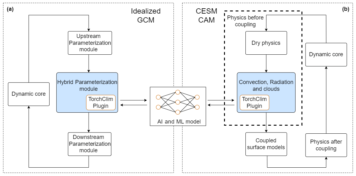
Figure 1An overview of the implementation of TorchClim into a GCM. (a) An idealized GCM, where a hybrid parameterization module calls TorchClim. To the GCM, it appears like any other parameterization module. (b) An elaboration of panel (a) for the reference implementation into CESM CAM, where the hybrid model replaces convection, radiation, and cloud parameterizations (adapted from Wang et al., 2022).
2.3 Parallelization considerations
One of the main dilemmas in introducing an ML and AI surrogate into the GCM involves parallelization. We note that most GCMs rely on CPUs to parallelize their execution and scale via MPI to multiple CPUs and compute nodes, while ML and AI frameworks tend to scale using GPUs. This creates a duplication of parallelization frameworks in the GCM, leading to the possibility that the CPUs will be idle while the GPUs access the surrogate model, and vice versa. Furthermore, there is an overhead in copying state from the CPU to the GPU, which could reduce the efficiency of this approach. It is possible that a better use of resources would be to use more CPUs to parallelize the GCM via MPI and keep the surrogate model on the same CPU core that is bound with the MPI rank. This is especially relevant to implementations that access the GPU serially or use a global MPI gather to push data to the GPU. At the least, users should be advised to benchmark their hybrid GCM against several architectures before running expensive workloads to ensure the best use of resources.
TorchClim offers the user the flexibility to choose between a pure CPU configuration (on the same CPU that the MPI rank resides) and one where the surrogate model is pushed to a GPU. Note that GPU functionality will be tested in the next release of TorchClim following the addition of vectorization of the MPI tile and configuration of multiple surrogate models (see Sect. 5). To achieve this flexibility, an instance of the TorchClim plugin is loaded at run-time to the thread-local storage (TLS) inside an MPI rank. This means that TorchClim's recommended best practice naturally follows the spatial discretization used to parallelize GCMs via CPU or MPI. This is illustrated in Fig. 2 for CAM, where the CPU or MPI parallelization discretizes the spatial domain into tiles and allocates each tile to a CPU. The instance of TorchClim lives inside the MPI rank associated with this CPU and can offload the requests to TorchClim to a range of parallelization options as supported by the underlying ML and AI framework.
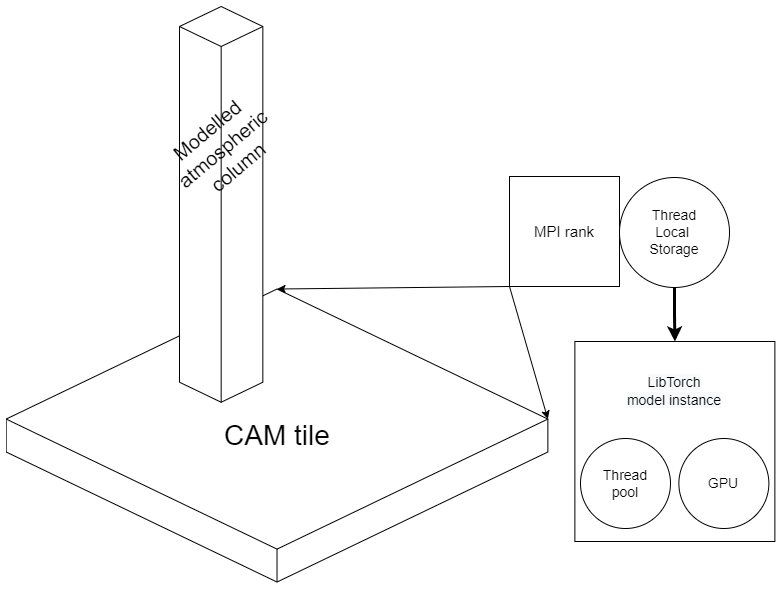
Figure 2An architecture diagram depicting the relationship between a GCM's physics geographical tile (chunk), representing a set of adjacent geographical grid locations, and a LibTorch instance. In a GCM with MPI support, both coexist within the MPI rank. LibTorch ML and AI models can subsequently execute on a local GPU or a thread pool.
We provide a reference implementation for the Community Atmospheric Model (Neale et al., 2010) that is part of CESM version 1.0.6. This comes in the form of a case study that demonstrates our recommended best practices outlined in Sect. 2.1. Specifically, this case study demonstrates:
-
how to include the TorchClim library into the GCM,
-
how to import the TorchClim module in Fortran,
-
how to call the plugin's interface,
-
how to pipe inputs and outputs from and to the GCM,
-
how to wrap the surrogate model as parameterization module, and
-
how to do basic validation and constraint tests.
Additional features that extend the functionality of the GCM and surrogate development cycle are discussed in Sect. 3.1 and 3.2.
Our case study's surrogate model is a DNN (described in Sect. 4.1) that predicts the total tendencies of moisture and heat due to moist processes (convection, clouds, and boundary layer) and radiation (Fig. 1b), thus replacing the respective TPs in CAM with a single surrogate model. Other parameterizations such as eddy diffusion, gravity wave drag, and CAM's dynamical core are left running as usual. Like many other GCMs, CAM uses MPI to discretize its domain, dividing the workload across processes and compute nodes. The physics parameterization suite in CAM divides the geographical domain into tiles of adjacent grid locations, with each tile associated with an MPI rank (process). Each grid location represents an atmospheric column in which the physics runs independently from other columns. This dictates the required spatial dimensions of the input and output of the surrogate model.
Our choice to replace the sum of moist and radiative physics parameterizations dictates the minimal set of output variables that the surrogate model will need to predict. Failing to predict and feed these back to the GCM can lead to run-time instabilities, regardless of the skill of the surrogate model. For example, Wang et al. (2022) found that direct and diffuse shortwave radiative variables must be predicted by their surrogate model. This is not surprising given that, in CAM, downstream surface models require these variables. The minimal set used in our case study, listed in Table 1, includes a subset of all the diagnostic variables the TPs produce, namely those required by the surrogate model or run-time diagnostics.
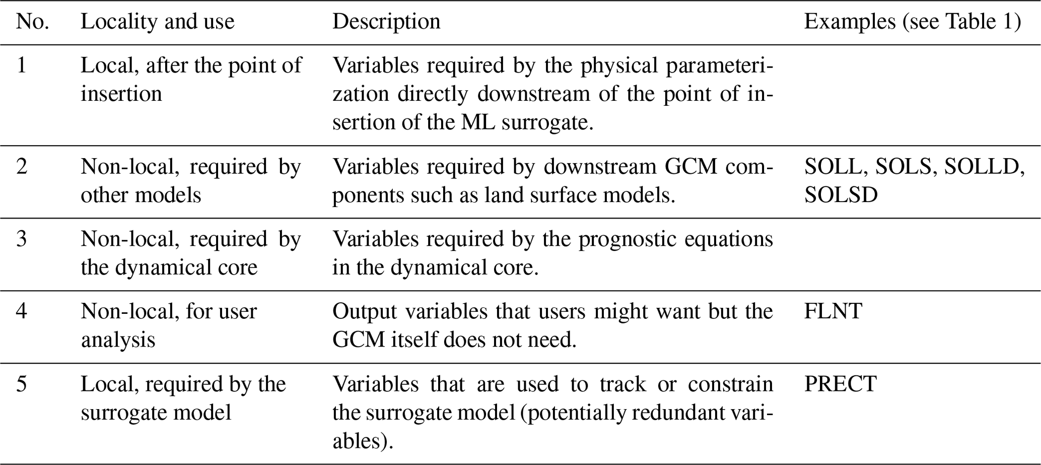
In developing our case study, we found that ensuring that output requirements are met can be a time-consuming task. To help users do this, Table 2 identifies several types of variables that are likely to be encountered along with their characteristics. The first three denote quantities that are needed either by the physics modules downstream of the surrogate model, by other climate system model components such as the land surface model, or by the dynamical core. Note that these types are not mutually exclusive. We also note here that, in principle, given appropriate training data, surrogate models could be developed to predict diagnostic quantities beyond those produced by the TPs (no. 4 in Table 2) – for example, simulated satellite radiances, paleoclimate proxies, downscaled meteorological fields, or even climate impacts. This important potential use case could allow such quantities to be produced more rapidly and efficiently than by current methods of offline calculation (which can have large storage requirements) or online simulators (which require effort to implement and affect GCM execution speed).
Table 1CAM history output variables used to train the ML and AI model. The input variables contain CAM prognostic variables and atmospheric boundary conditions, while the output dimension contains variables that are needed to comply with CAM’s interface downstream of the point of insertion of the NN model. Variables that are marked by the asterisk (*) are used for diagnostics and are not essential at run-time. Variables prefixed with “PREC” and “F” denote components of precipitation and radiation, respectively. Further description of variables can be found in CESM CAM history field documentation (Eaton, 2011).
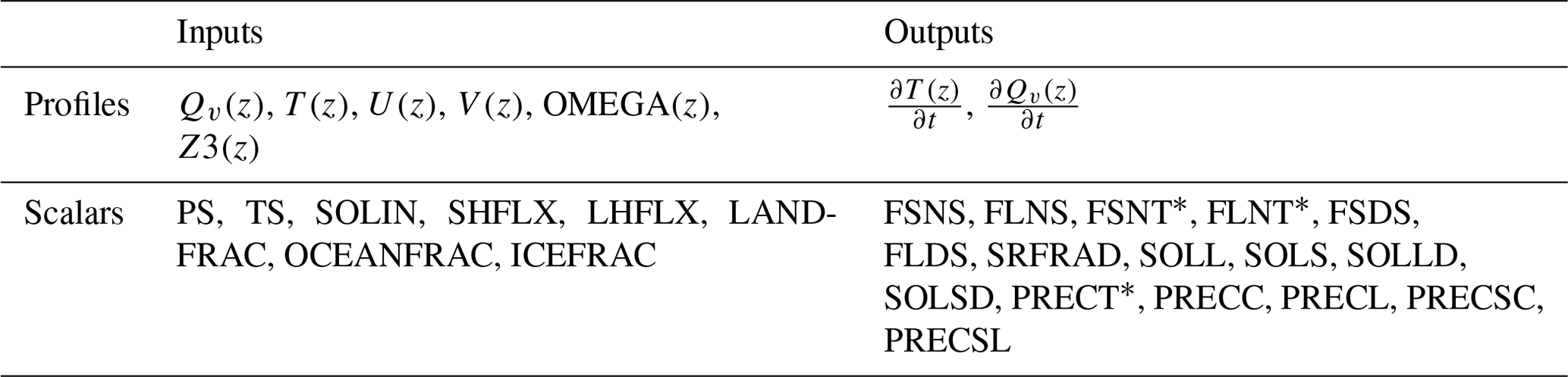
Table 2Hints designed to help the user identify the minimal set of output variables that a surrogate model needs to predict and pipe back into the GCM's workflow.
3.1 Alternate physics workflows
We recognize the potential of ML and AI to serve a range of modes of use. For example, users may wish to run an ML and AI surrogate only at a certain time step or within a particular geographical region. It is also desirable to be able to choose among multiple physics parameterizations that point to different surrogate model combinations. Alternatively, it may be desired to run multiple models side-by-side or as a replacement for different physics parameterizations. This functionality could also be used to diagnose instabilities in the surrogate model or do online corrections (e.g., Rasp, 2020), for example, by comparing the outputs from the surrogate model with the TP. The reference implementation supports this need by placing a mode selector before the call to the physics parameterization (Fig. 3). An advantage of this approach is that it offers users a way to extend CAM with new capabilities without removing existing ones. The reference implementation still offers the original parameterization of CAM alongside an ML and AI mode that runs combined moist and radiative parameterizations as an ML and AI surrogate and a dual mode that runs both of these side by side. Our implementation allows the user to achieve that out-of-the-box (without directly changing CESM CAM code base).
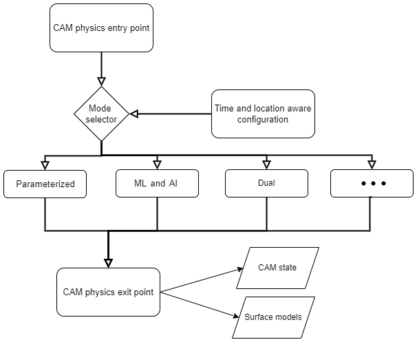
Figure 3A sketch of the mode selector, which allows the reference implementation to add new models of CAM physics alongside the original parameterization. The mode selector is placed before the entry point to CAM's physics parameterization, allowing the selector to choose the workflow for a given spatial and temporal location and use case. The selector facilitates fast turnover to extend CAM with additional physics workflows without compromising other workflows.
3.2 Assisting the learning phase
So far we assumed that an ML surrogate is available, without addressing where the data that would be used to train it would come from. A good starting point for training a surrogate model is simply to use the TP of the host GCM itself. In the reference implementation, this is the combined effect of the moist-physics and radiation parameterizations of CAM. This approach has the benefit that it allows us to benchmark a surrogate model both computationally and scientifically against an ideal synthetic dataset. It can also serve as a starting point for further training from other datasets that have missing or insufficient data, as is frequently the case with climate data. The user could mitigate learning biases in this using the TP as a starting point in different ways, for example, using an ensemble of TPs, potentially from different GCMs, or increasing the learning rate when training with subsequent data sources. To this end, the reference implementation of TorchClim is shipped with the export_state Fortran module. The user is provided with two subroutines: the first is inserted in the TP before the location where the surrogate model is to be called, while the second is inserted after that point. These produce a dataset of inputs and labels required for supervised learning. For example, our reference implementation replaces the parameterizations of moist physics and radiation, so these subroutines are placed in the TP before and after these parameterizations (Fig. 4). These add additional history variables to CAM's output, recording state and accumulated tendencies before and after the desired section of TPs.
This functionality could also be used to study instabilities during online runs of the GCM with the surrogate model. In our reference implementation, this can be done by extracting samples before and after the call to the surrogate model and tracking the locations where the surrogate model diverges from the TP offline.
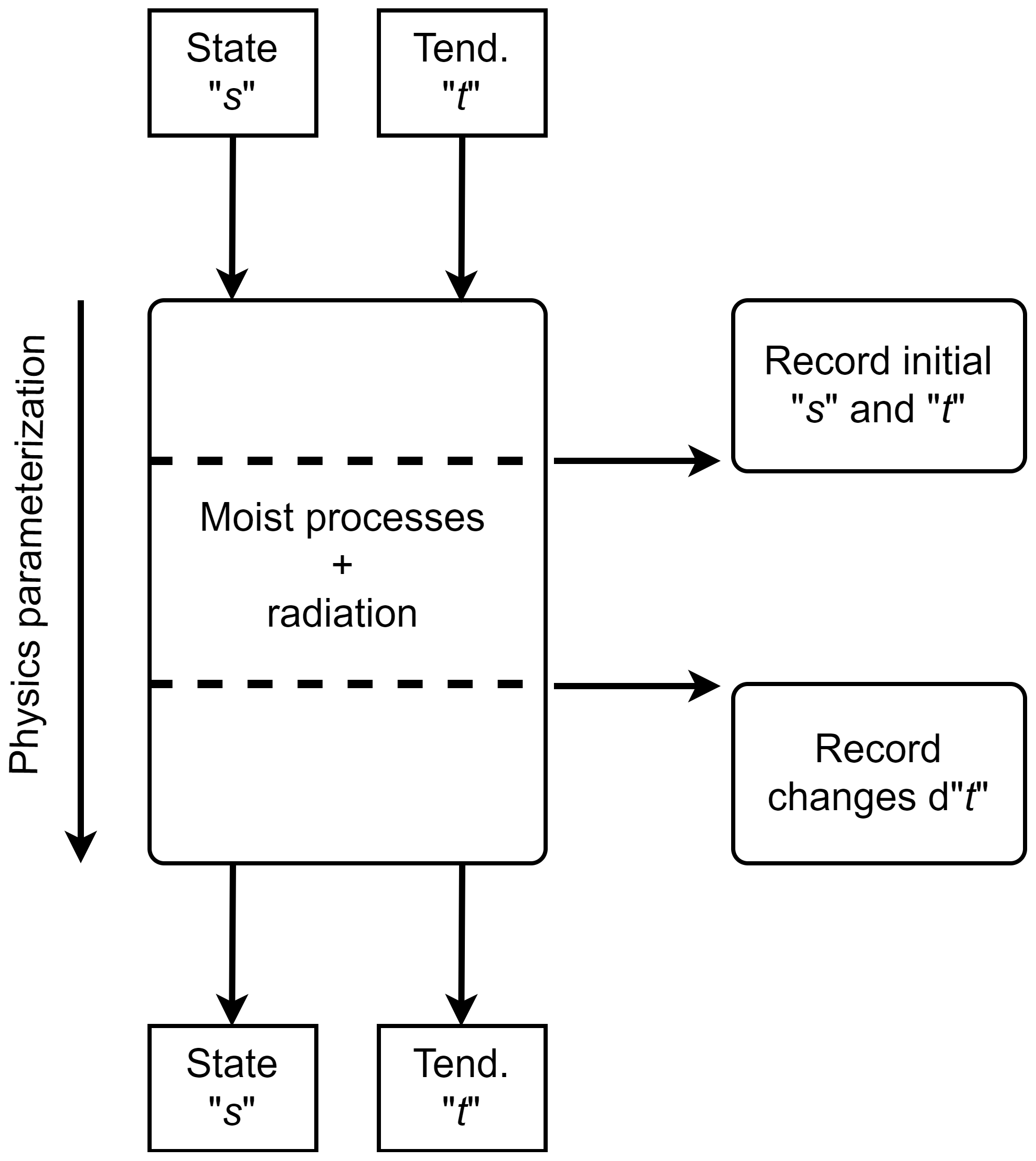
Figure 4The process of producing inputs and labels for supervised learning from the TP parameterization. Here we exemplify it using the TP of moist and radiative parameterization in CAM. The export_state module allows the user to take snapshots of CAM's physics state and tendencies before and tendencies after these TPs. These are saved to CAM's history files and subsequently used to train a baseline DNN (e.g., for our reference implementation).
We now evaluate the end-to-end process of outputting training data from the TP (described in Sect. 3.2), training a DNN offline, and then deploying this DNN as a surrogate inside CAM using TorchClim. In this case, success is evaluated on the computational performance and accuracy of the hybrid model relative to the original CAM, whose physics the DNN is emulating.
Since our reference implementation allows traditional and hybrid model versions to coexist under the same code base, it was used to produce the training dataset. We generated a 10-year run with this version of CAM using monthly AMIP sea surface temperatures (SSTs) (from 1979 to 1989). This run was configured to call the radiative parameterization at every model time step rather than hourly as in the original configuration. Likewise, it produced history outputs at every physical time step, allowing the training data to be composed of adjacent time steps for the inputs and outputs of the DNN. History variables were written for the state before and after the insertion point in CAM’s physics parameterization using the framework described in Sect. 3.2.
The first 9 years of this dataset were used for training and validation, and the last was used for testing. Training and validation samples were drawn uniformly over space and time, while testing data were sampled over time, using the entire spatial grid at a sampled time step. The training and validation sample size is proportional to the size of the time–space dimensions and matches or instances. This dataset was also randomly divided into 90 % training and 10 % validation datasets.
4.1 DNN surrogate model description
The DNN model for our case study was trained offline via PyTorch's Python interface. The input and output variables that the DNN used are discussed in Sect. 3 and shown in Table 1. These are composed of scalars such as radiative fluxes and vertical model level profiles (26 levels in this version of CAM).
The DNN is composed of seven fully connected layers. Each layer (except the last) is followed by a batch normalization, dropout, and a linear rectifier. We use the zero-mean or 1 standard deviation normalization per feature before the first layer, i.e., separately normalizing each model level (z) globally for each 3-D input variable, such as water vapor, and each 2-D variable (Table 1). Correspondingly, we use the 1 standard deviation re-normalization after the last layer for re-scaling the output during inference.
Equation (1) defines the loss function used to be minimized. The mean squared error (MSE) on the normalized output variables is the initial loss function to be minimized (LMSE). We also introduce additional terms in the loss function to address the biases described below. We add L2 regularization with a weight of one to all parameters except the biases and batch norm (LL2). Several constraints on range, equality, and conservation to prevent unphysical predictions are encoded as either parameterization of the outputs in the DNN model or as additional regularization terms in the optimization objective. These are defined for the three constraint groups discussed in Sect. 4.2 and Table 3. The loss trade-off coefficients α(⋅) are chosen experimentally.
Optimization is done using the Adam method (Kingma and Ba, 2014) with a learning rate of . We train for 100 epochs, with a large batch size of 24 × 96 × 144 atmospheric columns that are randomly selected in time and space from the original 10-year dataset. We determined 100 epochs to be a good compromise between model accuracy and training time on a separate validation set. Training beyond 100 epochs resulted only in marginal gains. Finally, we use linear warm-up for the first 10 % of epochs and cosine cool-down learning rate scheduler to zero.
During training, the validation data are used to monitor optimization progress and perform early stopping if necessary.
In practice, we tested dozens of versions of the DNN with various bug fixes and tweaks. This was made easy by the TorchClim interface which enables newly trained DNNs to be dropped in with no recompile of CAM required.
4.2 Constraining the target solution
Past studies and our own efforts have found that to obtain good performance, it is necessary to apply physical constraints to ML surrogates to prohibit nonphysical predictions (Beucler et al., 2021; Brenowitz et al., 2020; Mooers et al., 2021; Karniadakis et al., 2021).
In training the model for our reference implementation, we found a set of rules that helped constrain the target solution.
Here, we propose a classification of such constraints into three types, according to the nature of the applied constraint (Table 3).
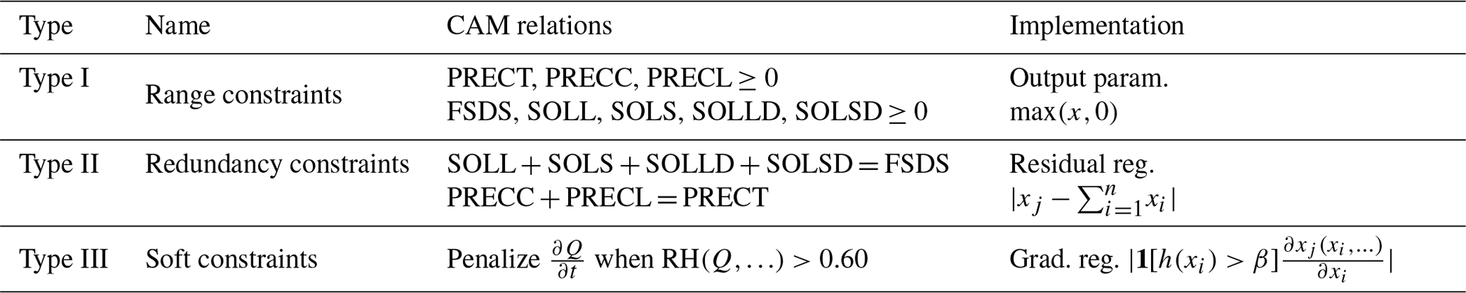
The variable x will usually be outputs of the surrogate but could also be inputs. Type I constraints stem from the fact that physical variables may be bounded in some way either by definition, a static threshold, or by another variable. For example, precipitation rate and shortwave radiation flux cannot be negative. Likewise, no component of shortwave radiation can exceed the incoming solar flux (given that plane-parallel radiation is assumed in CAM). The constraint, in this case, limits these variables to the space of solutions and , where SOLIN is solar insulation variable in CAM. We have found that ML approaches struggle to consistently obey this type of constraint to the required accuracy, especially since even small violations are unphysical and can cause problems elsewhere in the model; hence, we enforce the positivity constraint by applying the rectifier function to the output variables max(x,0). This is a type of inductive biasing (Karniadakis et al., 2021). Type II or “redundancy” constraints formalize a relation among variables, which generally means that the target solution exists on a manifold inside the unconstrained set of target solutions, i.e., there is physical redundancy in the output variables. For example, the sum of direct and diffuse shortwave radiation at the surface must be equal to the total radiation at the surface. Type II constraints, therefore, take the form , where xj is a surrogate output that consists of n components xi also represented by other surrogate outputs. To improve overall model learning, we incorporate these physically dictated constraints by converting them to a residual loss term in the objective , such that when the constraint is satisfied the residual will be zero. Note that such constraints could also be nonlinear. Type III or “soft” constraints penalize solutions that disobey a desired physical property expressed via functions of the output variables. For example, we expect that the sum of all tendencies of water vapor in a column will balance those of condensed water plus precipitation, but this relationship may not be exact due to small terms in the conservation equation (such as storage of condensed water) that are not known or available. Type III constraints are examples of learning biasing, following Karniadakis et al. (2021). As listed in Table 3, we implement a soft constraint that penalizes increasing moistening tendencies when relative humidity is above a specified threshold with gradient regularization term . This term will penalize positive slopes, i.e., gradients of the output variable xj with respect to input variable xi but only when h(xi)>β. In this example, xj is the moistening tendency, xi is the input humidity, and h() is the relative humidity function.
Naively, these constraints could just be applied at run-time in the GCM's integration. For example, one might truncate a precipitation variable to be non-negative at run-time. Adding these constraints to the learning stage, however, can assist in learning the joint solution rather than correcting a single variable. For example, if the learning process had predicted negative precipitation, this may imply non-physical predictions of other variables that are empirically related to precipitation even if no other constraints are violated. To ameliorate this issue, we bring Type I–III constraints into the learning stage, presenting them as additional terms in the loss function. Type I constraints are also applied at run-time, since learning does not completely eliminate violations, and even small Type I violations (for example negative solar fluxes) can crash the land model.
4.3 The skill of the hybrid CAM ML model
We evaluate the hybrid CAM ML model by comparing it with standard CAM, whose physics the surrogate emulates. We do not perform an extensive skill evaluation, since our main objective is to test the plugin rather than the skill of the NN physics emulator, which can easily be changed. Here we present results from a hybrid CAM ML run that starts from the same starting point that was used for extract the training data. That is the CESM Atmospheric Model Intercomparison Project (AMIP) scenario for CAM4 with default configuration parameters. The hybrid CAM ML model was able to run for 6 months before exhibiting numerical instabilities. These instabilities appear to be brought on by stratospheric drift which we have not yet attempted to correct. Here we present results for the fifth month into the run, before the instabilities became apparent. During this month, the hybrid model produces zonal mean moisture and temperature tendencies that closely resemble those of the original model (Fig. 5). The Inter-Tropical Convergence Zone (ITCZ) is slightly too narrow, and there is a double-ITCZ bias in the hybrid model and too much heating near the tropopause, but the differences overall appear modest. The hybrid model also shows similar temporal variations in tropical variability and waves when comparing them to the original CAM model (Fig. 6). This is a stronger test of the surrogate model, since the character of tropical waves is sensitive to the behavior of moist physics (Majda and Khouider, 2002; Kelly et al., 2017). Note that the initial behavior of the hybrid model matches that obtained with CAM parameterizations, diverging later, as expected, but retaining a similar character. Despite spatiotemporal pattern similarities, the hybrid model exhibits larger relative humidity extremes (Fig. 6). It is not clear why these extremes are permitted by the surrogate model, although earlier versions of the model that lacked the relative humidity (RH) sensitivity regularization (Sect. 4.2) showed a more severe manifestation of the problem, suggesting that even with regularization, the surrogate model is insufficiently quick in the condensation of water above saturation compared to the CAM physics. This is not too surprising, as the parameterized physics is extremely nonlinear, and we have not explicitly coded the Clausius–Clapeyron relation into the DNN, so it must learn the point at which condensation (rapidly) begins. Thus, we expect that better use of physics-informed architectures or other improvements would lead to further improvement in emulation skill.
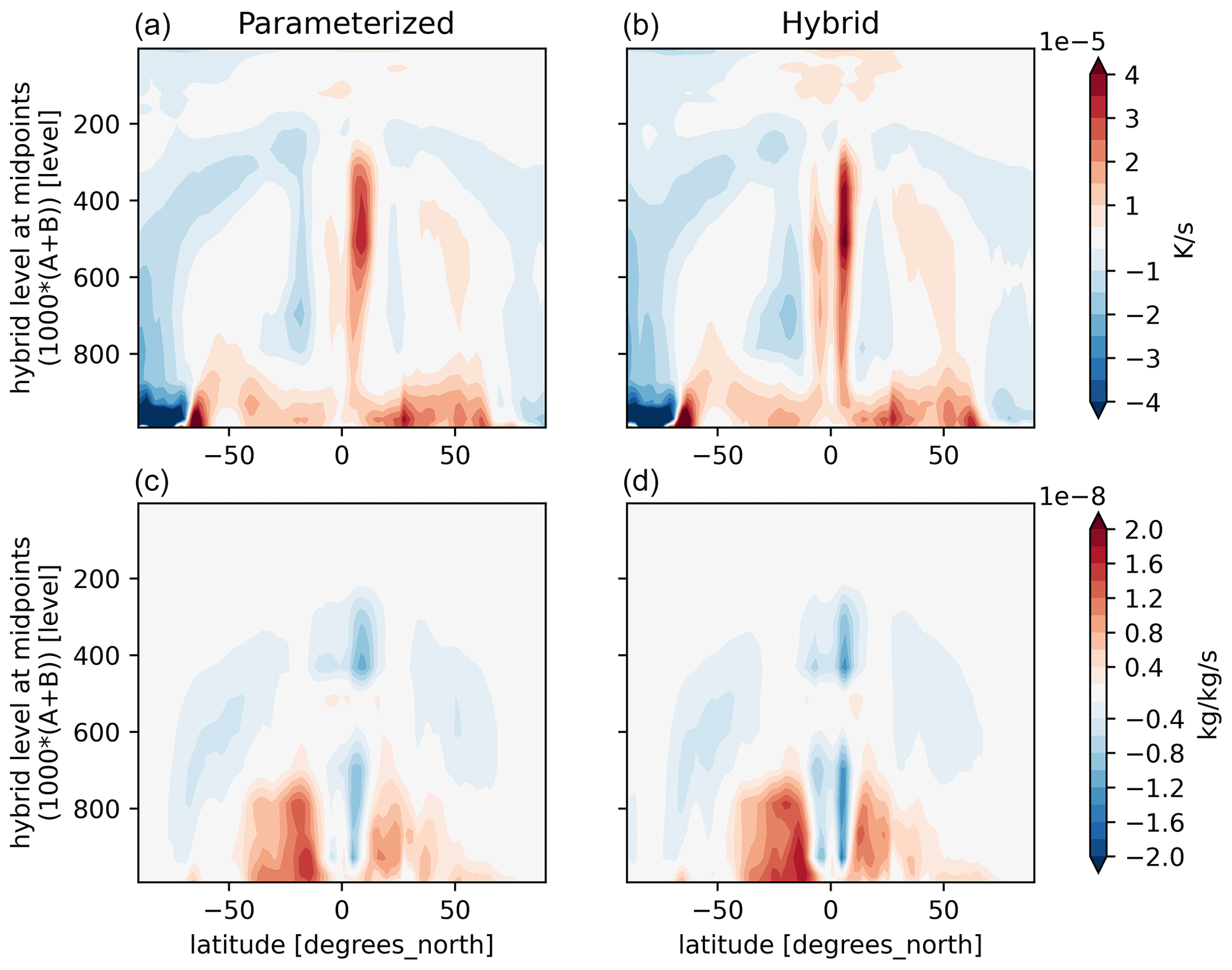
Figure 5Zonal mean specific humidity and temperature tendencies in the fifth month after the start of the simulation. The original parameterized CAM (a, c) and the hybrid CAM ML, where CAM is coupled with the surrogate model using TorchClim (b, d), are shown.
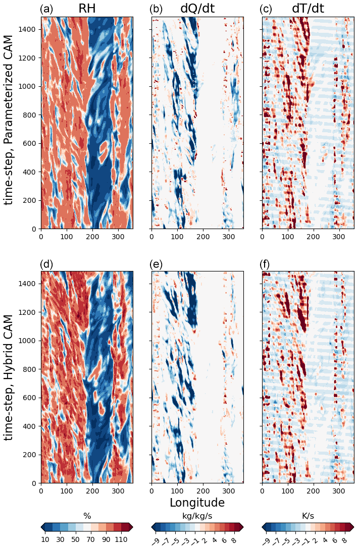
Figure 6Predicted values vs. longitude and time during the fifth month after the start of the simulation at hybrid model level 233 at the Equator (approximately 233 hPa). The original parameterized CAM (a–c) and the hybrid CAM ML, where CAM is coupled with the surrogate model using TorchClim (d–f), are shown. (a–f) Relative humidity, specific humidity tendencies, and temperature tendencies. The y axis denotes the model physics time step (which is 30 min).
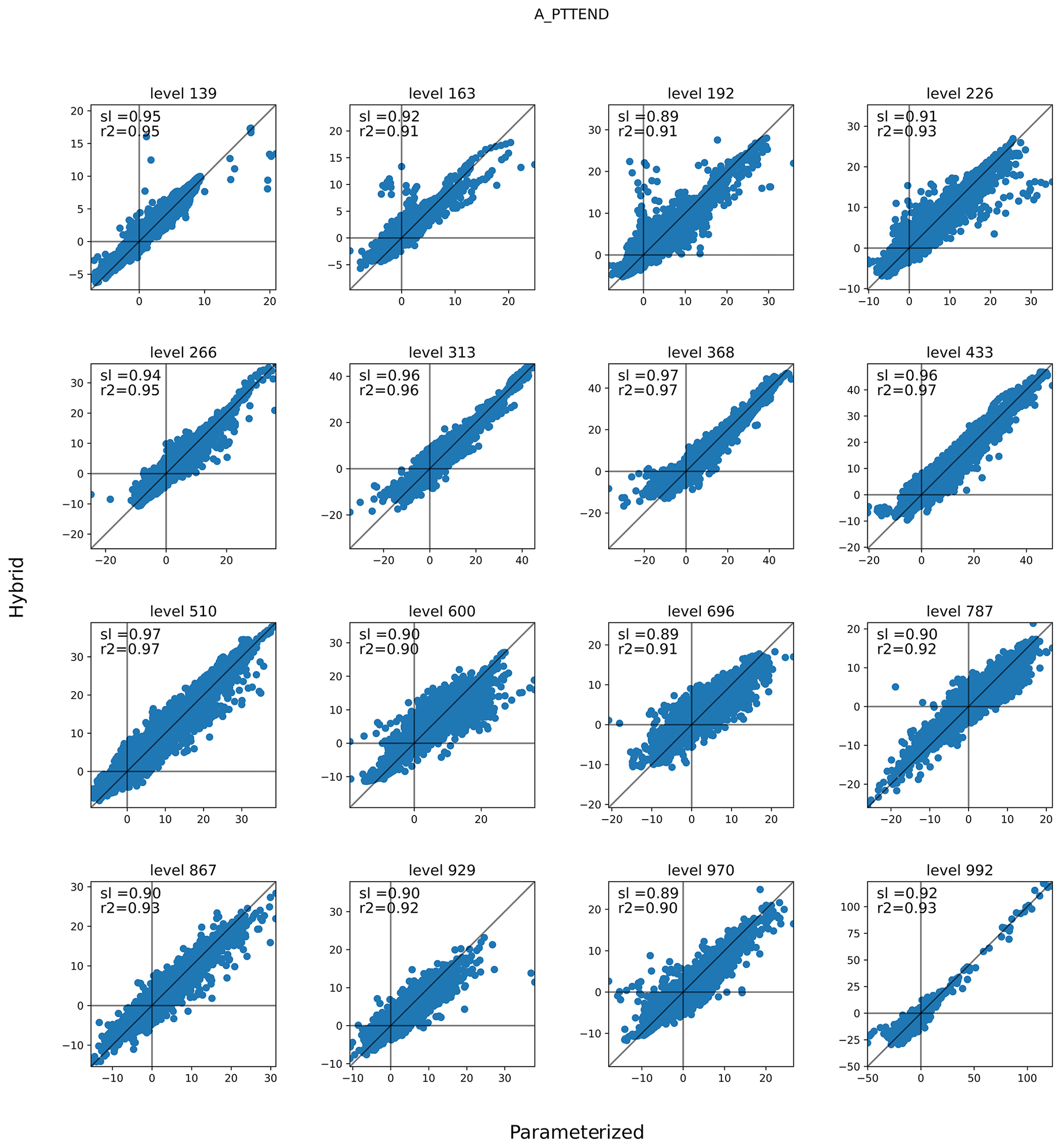
Further insights into the behavior of the hybrid model are gained using the third mode of operation of TorchClim, where the ML model is called alongside the original parameterization of CAM. Here we call the ML model and output its response without assimilating it into the CAM workflow. Figures 7–8 compare specific humidity and temperature tendencies of the original CAM parameterization to the ones from the ML model at various vertical levels between 10° N and 10° S from the Equator. A perfect ML model would follow the 1:1 line. Both specific humidity and temperature tendencies exhibit a line of best fit that is smaller than one. The ML model generally predicts smaller positive specific humidity tendencies (Fig. 7). Interestingly, for both quantities, the lowest skill is found in the mid-troposphere between hybrid model levels 510 and 696. At these levels, the ML model learns the spurious features of specific humidity tendencies that do not exist in the original model. These discrepancies appear at vertical levels where shallow convection is active and are in line with Mooers et al. (2021), who found that their deterministic DNN had less skill in regions with fast stochastic convective activity. However, this issue could also be attributed to the fact that cloud liquid and ice are not treated by the current surrogate DNN model.
Although these biases could be discovered offline during training, we found that the ability of TorchClim to run the original and hybrid CAM models side by side enabled us to quickly diagnose errors in hybrid simulations, particularly where there may not be analogs in the training dataset.
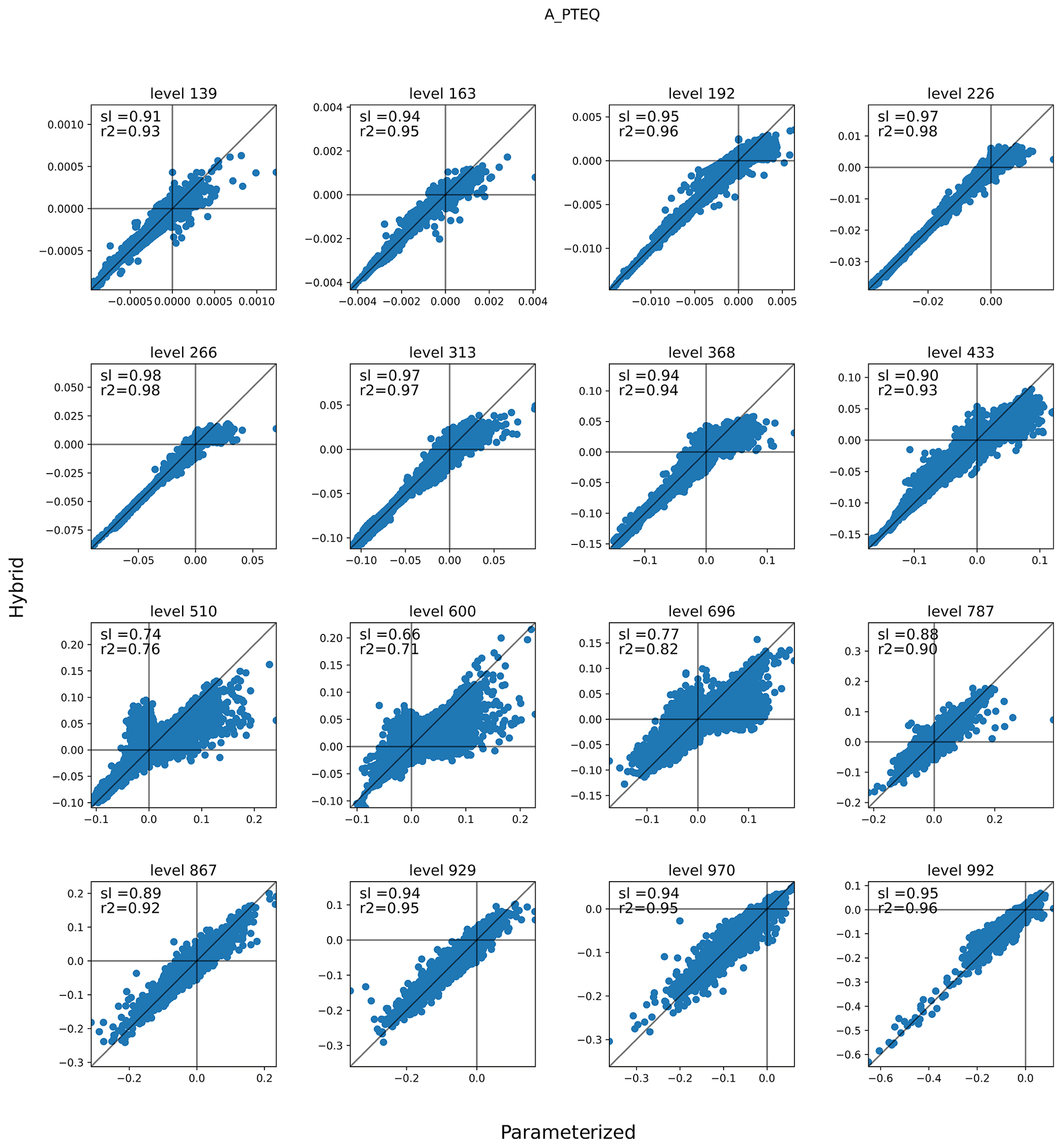
Figure 7Specific humidity tendencies (kg kg−1 d−1 × 10) of the original cam parameterization (x axis) and the hybrid CAM ML parameterization (y axis) for various vertical levels on day 10 of the run. Calls to the ML model were done from within the integration loop of the original CAM parameterizations. Black lines denote the origins and the 1:1 line. The hybrid model level is denoted in the title, while the slope (sl) and r2 are printed inside each panel.
4.4 Computational performance
The evaluation of computing speed is undertaken on the normal queue of the Gadi infrastructure in the National Computational Infrastructure (NCI), supported by the Australian Government. The normal queue nodes are based on 2 × 24 core Intel Xeon Platinum 8274 (Cascade Lake) 3.2 GHz CPUs, with 192 GB RAM, two CPU sockets, each with two NUMA (non-uniform memory access) nodes, and no hyper-threading. Noticeably, MPI ranks are bound to the core, with each MPI rank hosting an instance of the DNN model.
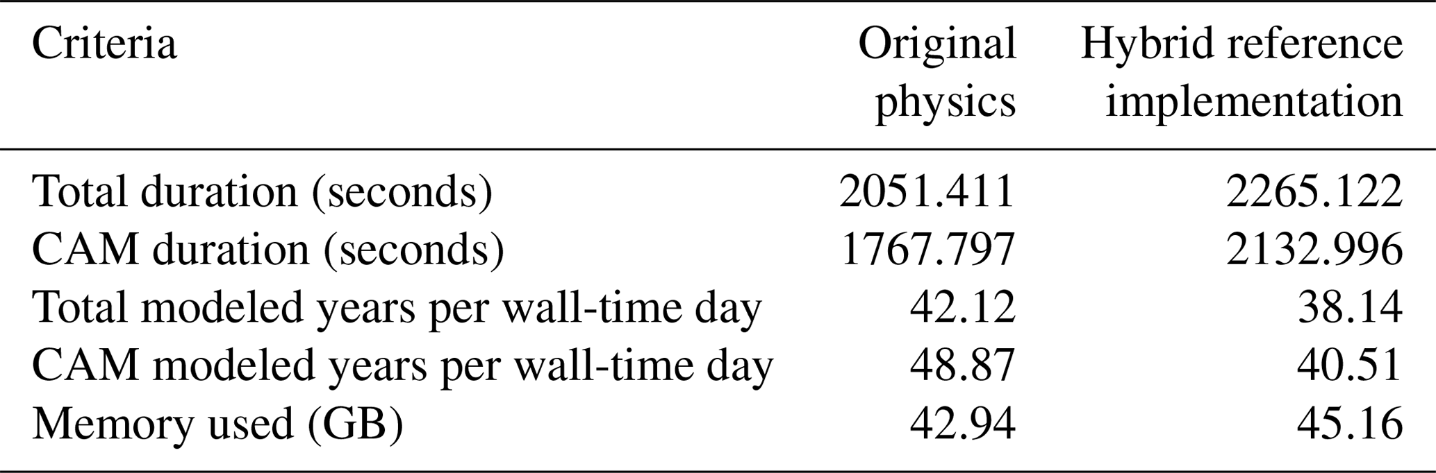
For the sake of comparison, both original and hybrid CAM configurations were run for a year with minimal monthly mean output variables so that a relatively large fraction of the overall CPU would be spent on computation. Each run used three nodes on the normal queue (144 CPU cores) and 64 GB RAM. This configuration matched the number of longitudes of our AMIP scenario spatial discretization. The hybrid and standard configurations of the GCM required similar resources, unlike previous implementations we know of, where the DNN implementation required significantly more compute resources than the original model. The results of this experiment are detailed in Table 4. The hybrid model added 20 % to the wall-time of CAM, reducing its performance by 8 modeled years per wall-time day. The total CESM speed degraded by 10 %, which amounted to 4 modeled years per wall-time day. The addition of ML and the AI model added only about 5 % (2 GB) to the overall memory requirements.
Since our setup is similar to Wang et al. (2022), it is convenient to compare the performance of these approaches. Wang et al. (2022) used a similar 1.9 × 2.5° grid resolution and 30 instead of 26 vertical levels but used CAM5, which is about 4 times slower than CAM4. Noting uncertainties regarding the computational complexities of the DNNs of each implementation, their configuration was able to produce 10 modeled years per wall-time day, which is comparable to the performance of our reference implementation. However, their approach used 25 % more CPU cores, Intel's Math Kernel Library optimization, and additional dedicated hardware (GPU and storage). We also note that our own results were achieved before any optimization (such as vectorizing the calls per geographical tile, pre-allocating of memory buffers, and using GPUs). In developing future versions of TorchClim, we anticipate vectorizing the calls to the surrogate DNN model, pre-allocating and re-using data structures, and considering automatically offloading to a GPU when available. It is expected that, despite each MPI rank hosting a single thread, the performance improvements in vectorization and pre-allocation will be significant (even without GPUs or multi-threading). For example, assuming that vectorization will match the spatial tile (chunk in CAM's terminology), the reduction in heap memory allocations calls will be of the order of , where denotes the number of atmospheric columns of the tile (thus being more important for larger tiles in terms of the number of grid locations per tile).
Table 4Run-time performance for CESM total run-time and the atmospheric component (CAM) only.
4.5 How might TorchClim help with stability issues
Stability issues take a considerable portion of surrogate model development. Past efforts have found that stability can vary unpredictably among similarly constructed surrogate models, indicating a need to understand this for hybrid modeling to progress (Wang et al., 2022; Brenowitz et al., 2020). We list the ways in which the TorchClim approach could help.
-
Our use of data from a TP to train a surrogate model seems like an ideal test bed to study online stability issues that arise due to imperfect emulation.
-
The mode selector (Sect. 3.1) allows the TP and the surrogate model to be run side by side, which could help catch or correct issues online during the GCM run.
-
The data extraction tool (Sect. 3.2) also allows training samples to be extracted with both the surrogate and TP predictions side by side, providing the option to study instabilities offline. These could also be used to re-train the surrogate model to mitigate specific instabilities.
-
The TorchClim plugin can be used as a separate executable, allowing changes to the interface to be tested outside the GCM.
We note that the last two of these possibilities helped us ensure that the integration between the plugin and surrogate models matches to inference via Python.
5.1 ONNX support
The current version of TorchClim is able to import surrogate models that were saved through PyTorch's scripting infrastructure. A natural extension of that is to allow the use of the ONNX interface to imports. With the maturity of ONNX, this would improve performance while allowing us to use the ML and AI framework beyond PyTorch.
5.2 Stateful ML and AI models
A stateful AI and ML model preserves an internal state between one call to another, for example, in the case of agent-based algorithms such as reinforcement learning. In the case of GCMs, a specific instance of surrogate model, compute node, and GPU may be associated with an MPI rank. However, a standing issue with MPI applications is the need to optimize their performance on a given infrastructure. In the age of non-uniform memory architectures (NUMA), this tends to be achieved via binding (affinity) instructions that communicate with the underlying infrastructure the required binding of MPI ranks. For example, many applications require binding to cores, memory, or cache to achieve the best performance. The case of the stateful ML and AI model brings in an additional challenge. In this case, an instance of the ML and AI model holds an internal state that is bound to a given geographical location. This has two consequences.
-
A geographical location in the GCM needs to be mapped to an instance of the ML and AI model, which is mapped to a specific thread.
-
The instance of the ML and AI model (and state) is bound to a given GPU if the ML and AI model uses GPUs at the GCM run-time.
The consequence of this is the binding of a geographical location or tile to a resource (thread and GPU). An implementation of this feature requires TorchClim to retain a mapping between a GPU and a geographical location and for the GCM to bind the geographical location (tile) to a CPU. Since the latter requirement is GCM-specific, its implementation of these is out of scope in the current reference implementation.
5.3 Vectorization and pre-allocation
The current implementation is shipped without optimization. Despite that, our experiments with the reference implementation into CESM CAM exhibit good performance. Beyond that, the framework is desired to automate the vectorization of calls to underlying surrogates. In addition, the framework should pre-allocate all the buffers required to interact with LibTorch. These improvements are expected to have a significant effect on performance even without the use of GPUs.
5.4 Multiple surrogate models
The reference implementation does not support multiple surrogate models within the same run. However, the extension of the TorchClim framework to support multiple surrogate models is straightforward.
A new direction in climate modeling has recently opened with the development of hybrid climate models, where physical schemes are represented by machine-learned surrogates. Previous efforts in this direction have focused on the accuracy of surrogates and the potential benefits of rapid execution speed for inexpensively emulating high-resolution models. We argue that for this direction to bear fruit, implementations be will required that can achieve acceptable performance on two additional fronts, namely flexibility and scalability in the use of software and hardware resources and ease of surrogate implementation and replacement. These need to take into account the vast investment in existing GCMs.
To this End, we propose a set of best-practice requirements and features to guide hybrid model implementations, including ease of use and flexibility with computational performance in a plug-and-play-like fashion, where the plugin does not need to be recompiled due to changes in the surrogate model. We then present a plugin and reference implementation, TorchClim, that demonstrates these principles and facilitates the introduction of ML- and AI-based models into GCMs. It focuses on offering a robust and scalable way to do this, addressing a key gap in current practices. The plugin can be loaded and used from any component in the GCM and expose itself as any other parameterization. The approach can support any number of surrogate models simultaneously, while surrogate models can be loaded without the need to recompile the plugin. This is offered as a community-based, open-source project (see the Code and data availability section below).
Though TorchClim may have a wider range of applications, it aims to offer a data-driven approach to physics parameterizations. To this end, we implement a proof of concept into CAM physics, replacing parameterizations of moist and radiative parameterizations with a call to TorchClim. We test this by creating a surrogate model that was learned using CAM data. In doing so, we found the need to assist the learning process to find stable, physically motivated surrogate models. This was done by introducing constraints as added loss terms during the training stage. To aid further efforts, we have generalized these insights into a set of guidelines that could be reused for other learning tasks and a set of guidelines that help introduce surrogate models into a GCM. Our implementation was able to run for 6 months before exhibiting numerical instabilities associated with temperature drift at upper levels. We believe that this issue is due to the surrogate training and lack of relaxation of the stratosphere, both of which are under continued investigation, rather than integration issues which led to much more rapid instabilities before they were resolved. Following this approach, the hybrid model, running on the same hardware as the standard CAM and without the optimization of the TorchClim plugin, performed reasonably well in terms of accuracy and significantly better in terms of compute resources compared to other hybrid models in the literature that included an interactive land surface as done here. Its computational performance is currently similar to that of the original CAM4, which might seem as though nothing has been gained. CAM4 is, however, a fast model which can easily accommodate multicentennial simulations; the promise of ML is to eventually improve the fidelity of such models without significantly increasing their cost. A premise here is that DNNs of a similar complexity and execution speed to that tested here but trained on superior data (for example, from much higher-resolution models) could achieve such improvements or, alternatively, that experimentation with a diverse suite of surrogates could lead to greater understanding of the parameterization challenge. We also note that the computational performance could be improved with vectorization and the use of additional dedicated hardware.
We anticipate that the flexibility and speed offered by the TorchClim principles and implementation will help unlock the full potential of AI and ML in advancing climate modeling by allowing rapid testing of diverse surrogates to learn from their online performance, as well as their offline performance. Future extensions should consider training using other data sources in order to improve on existing traditional parameterizations or enable the efficient delivery of new output variables from climate models at run-time, such as impact measures or comparisons to observing platforms such as satellites or indirect climate proxy data from geologic archives. Our tests with CESM CAM suggest that the incorporation of TorchClim to other parameterizations, later versions of CESM, and even other GCMs is relatively straightforward. Our hope is that such a framework will serve as a stepping stone to solving persisting gaps in GCMs.
The TorchClim framework is available at https://doi.org/10.5281/zenodo.8390519 (Fuchs et al., 2023a, current version). User and installation manuals can be found in the README.md file of the project. Further development effort of TorchClim is tracked at https://github.com/dudek313/torchclim (last access: 5 April 2024). Scripts and data for the figures in this work are available upon request from the corresponding authors.
All authors contributed to the development of ideas and writing of the paper. SCS designed the initial experiments with contributions from all the authors. SCS, KT, AP, and DF developed the final format of the TorchClim framework and its reference implementation. KT implemented and tuned the DNN, and DF and AP ran the simulations that produced the inputs for the DNN, as well as the test runs with the surrogate model.
The contact author has declared that none of the authors has any competing interests.
Publisher’s note: Copernicus Publications remains neutral with regard to jurisdictional claims made in the text, published maps, institutional affiliations, or any other geographical representation in this paper. While Copernicus Publications makes every effort to include appropriate place names, the final responsibility lies with the authors.
This work has been partly funded by the DARPA ACTM Program. The computational support and infrastructure have been provided by the Australian National Computational Infrastructure and the Computational Modeling Support team at the Climate Change Research Centre/University of New South Wales.
This research has been supported by the Defense Advanced Research Projects Agency (ACTM Program).
This paper was edited by Mohamed Salim and reviewed by three anonymous referees.
Beucler, T., Pritchard, M., Rasp, S., Ott, J., Baldi, P., and Gentine, P.: Enforcing Analytic Constraints in Neural Networks Emulating Physical Systems, Phys. Rev. Lett., 126, 098302, https://doi.org/10.1103/PhysRevLett.126.098302, 2021. a, b, c
Bi, K., Xie, L., Zhang, H., Chen, X., Gu, X., and Tian, Q.: Accurate medium-range global weather forecasting with 3D neural networks, Nature, 619, 533–538, 2023. a
Brenowitz, N. D. and Bretherton, C. S.: Spatially Extended Tests of a Neural Network Parametrization Trained by Coarse-Graining, J. Adv. Model. Earth Sy., 11, 2728–2744, https://doi.org/10.1029/2019MS001711, 2019. a, b, c
Brenowitz, N. D., Beucler, T., Pritchard, M., and Bretherton, C. S.: Interpreting and Stabilizing Machine-Learning Parametrizations of Convection, J. Atmos. Sci., 77, 4357–4375, https://doi.org/10.1175/JAS-D-20-0082.1, 2020. a, b, c
Dunbar, O. R. A., Garbuno-Inigo, A., Schneider, T., and Stuart, A. M.: Calibration and Uncertainty Quantification of Convective Parameters in an Idealized GCM, J. Adv. Model. Earth Sy., 13, e2020MS002454, https://doi.org/10.1029/2020MS002454, 2021. a
Eaton, B.: User's guide to the Community Atmosphere Model CAM-5.1, NCAR, http://www.cesm.ucar.edu/models/cesm1.0/cam (last access: 1 January 2020), 2011. a
Fuchs, D., Sherwood, S. C., Prasad, A., Trapeznikov, K., and Gimlett, J.: TorchClim v1.0: A deep-learning framework for climate model physics, Zenodo [code and data set], https://doi.org/10.5281/zenodo.8390519, 2023a. a, b
Fuchs, D., Sherwood, S. C., Waugh, D., Dixit, V., England, M. H., Hwong, Y.-L., and Geoffroy, O.: Midlatitude Jet Position Spread Linked to Atmospheric Convective Types, J. Climate, 36, 1247–1265, https://doi.org/10.1175/JCLI-D-21-0992.1, 2023b. a
Gentine, P., Pritchard, M., Rasp, S., Reinaudi, G., and Yacalis, G.: Could Machine Learning Break the Convection Parameterization Deadlock?, Geophys. Res. Lett., 45, 5742–5751, https://doi.org/10.1029/2018GL078202, 2018. a
Geoffroy, O., Sherwood, S. C., and Fuchs, D.: On the role of the stratiform cloud scheme in the inter-model spread of cloud feedback, J. Adv. Model. Earth Sy., 9, 423–437, https://doi.org/10.1002/2016MS000846, 2017. a
Grise, K. M. and Polvani, L. M.: Southern Hemisphere Cloud–Dynamics Biases in CMIP5 Models and Their Implications for Climate Projections, J. Climate, 27, 6074–6092, https://doi.org/10.1175/JCLI-D-14-00113.1, 2014. a
Howland, M. F., Dunbar, O. R. A., and Schneider, T.: Parameter Uncertainty Quantification in an Idealized GCM With a Seasonal Cycle, J. Adv. Model. Earth Sy., 14, e2021MS002735, https://doi.org/10.1029/2021MS002735, 2022. a
IPCC: Climate Change 2021: The Physical Science Basis. Contribution of Working Group I to the Sixth Assessment Report of the Intergovernmental Panel on Climate Change, edited by: Masson-Delmotte, V., Zhai, P., Pirani, A., Connors, S. L., Péan, C., Berger, S., Caud, N., Chen, Y., Goldfarb, L., Gomis, M. I., Huang, M., Leitzell, K., Lonnoy, E., Matthews, J. B. R., Maycock, T. K., Waterfield, T., Yelekçi, O., Yu, R., and Zhou, B., Cambridge University Press, Cambridge, United Kingdom and New York, NY, USA, 2391 pp., https://doi.org/10.1017/9781009157896, 2021. a
Karniadakis, G. E., Kevrekidis, I. G., Lu, L., Perdikaris, P., Wang, S., and Yang, L.: Physics-informed machine learning, Nature Reviews Physics, 3, 422–440, https://doi.org/10.1038/s42254-021-00314-5, 2021. a, b, c
Kelly, P., Mapes, B., Hu, I.-K., Song, S., and Kuang, Z.: Tangent linear superparameterization of convection in a 10 layer global atmosphere with calibrated climatology, J. Adv. Model. Earth Sy., 9, 932–948, https://doi.org/10.1002/2016MS000871, 2017. a, b
Kingma, D. P. and Ba, J.: Adam: A Method for Stochastic Optimization, arXiv [preprint], https://doi.org/10.48550/ARXIV.1412.6980, 2014. a
Majda, A. and Khouider, B.: Stochastic and mesoscopic models for tropical convection, P. Natl. Acad. Sci. USA, 99, 1123–1128, https://doi.org/10.1073/pnas.032663199, 2002. a
Mooers, G., Pritchard, M., Beucler, T., Ott, J., Yacalis, G., Baldi, P., and Gentine, P.: Assessing the Potential of Deep Learning for Emulating Cloud Superparameterization in Climate Models With Real-Geography Boundary Conditions, J. Adv. Model. Earth Sy., 13, e2020MS002385, https://doi.org/10.1029/2020MS002385, 2021. a, b, c
Neale, R. B., Chen, C.-C., Gettelman, A., Lauritzen, P. H., Park, S., Williamson, D. L., Conley, A. J., Garcia, R., Kinnison, D., Lamarque, J.-F., Mills, M. J., Tilmes, S., Morrison, H., Cameron-Smith, P., Collins, W. D., Iacono, M. J., Easter, R. C., Liu, X., Ghan, S. J., Rasch, P. J., and Taylor, M. A.: Description of the NCAR community atmosphere model (CAM 5.0), NCAR Tech. Note NCAR/TN-486+ STR, 1–12, https://doi.org/10.5065/wgtk-4g06, 2010. a
Nuijens, L., Medeiros, B., Sandu, I., and Ahlgrimm, M.: Observed and modeled patterns of covariability between low-level cloudiness and the structure of the trade-wind layer, J. Adv. Model. Earth Sy., 7, 1741–1764, https://doi.org/10.1002/2015MS000483, 2015. a
O'Gorman, P. A. and Dwyer, J. G.: Using Machine Learning to Parameterize Moist Convection: Potential for Modeling of Climate, Climate Change, and Extreme Events, J. Adv. Model. Earth Sy., 10, 2548–2563, https://doi.org/10.1029/2018MS001351, 2018. a
Paszke, A., Gross, S., Massa, F., Lerer, A., Bradbury, J., Chanan, G., Killeen, T., Lin, Z., Gimelshein, N., Antiga, L., Desmaison, A., Kopf, A., Yang, E., DeVito, Z., Raison, M., Tejani, A., Chilamkurthy, S., Steiner, B., Fang, L., Bai, J., and Chintala, S.: PyTorch: An Imperative Style, High-Performance Deep Learning Library, in: Advances in Neural Information Processing Systems 32, 8024–8035, Curran Associates, Inc., http://papers.neurips.cc/paper/9015-pytorch-an-imperative-style-high-performance-deep-learning-library.pdf (last access: 8 December 2019), 2019. a
Rampal, N., Gibson, P. B., Sood, A., Stuart, S., Fauchereau, N. C., Brandolino, C., Noll, B., and Meyers, T.: High-resolution downscaling with interpretable deep learning: Rainfall extremes over New Zealand, Weather and Climate Extremes, 38, 100525, https://doi.org/10.1016/j.wace.2022.100525, 2022. a
Rasp, S.: Coupled online learning as a way to tackle instabilities and biases in neural network parameterizations: general algorithms and Lorenz 96 case study (v1.0), Geosci. Model Dev., 13, 2185–2196, https://doi.org/10.5194/gmd-13-2185-2020, 2020. a, b
Satoh, M., Stevens, B., Judt, F., Khairoutdinov, M., Lin, S.-J., Putman, W. M., and Duben, P.: Global Cloud-Resolving Models, Current Climate Change Reports, 5, 172–184, https://doi.org/10.1007/s40641-019-00131-0, 2019. a
Schneider, T., Lan, S., Stuart, A., and Teixeira, J.: Earth System Modeling 2.0: A Blueprint for Models That Learn From Observations and Targeted High-Resolution Simulations, Geophys. Res. Lett., 44, 12396–12417, https://doi.org/10.1002/2017gl076101, 2017. a, b
Simpson, I. R., McKinnon, K. A., Kennedy, D., Lawrence, D. M., Lehner, F., and Seager, R.: Observed humidity trends in dry regions contradict climate models, P. Natl. Acad. Sci. USA, 121, e2302480120, https://doi.org/10.1073/pnas.2302480120, 2024. a
Wang, X., Han, Y., Xue, W., Yang, G., and Zhang, G. J.: Stable climate simulations using a realistic general circulation model with neural network parameterizations for atmospheric moist physics and radiation processes, Geosci. Model Dev., 15, 3923–3940, https://doi.org/10.5194/gmd-15-3923-2022, 2022. a, b, c, d, e, f, g, h
Watt-Meyer, O., Brenowitz, N. D., Clark, S. K., Henn, B., Kwa, A., McGibbon, J., Perkins, W. A., and Bretherton, C. S.: Correcting Weather and Climate Models by Machine Learning Nudged Historical Simulations, Geophys. Res. Lett., 48, e2021GL092555, https://doi.org/10.1029/2021GL092555, e2021GL092555 2021GL092555, 2021. a
Wikipedia: Moore's Law, Wikipedia, https://en.wikipedia.org/wiki/Moore's_law (last access: 5 July 2024), 2022. a
Yuval, J. and O'Gorman, P. A.: Stable machine-learning parameterization of subgrid processes for climate modeling at a range of resolutions, Nat. Commun., 11, 3295, https://doi.org/10.1038/s41467-020-17142-3, 2020. a
Zelinka, M. D., Myers, T. A., Mccoy, D. T., Po-Chedley, S., Caldwell, P. M., Ceppi, P., Klein, S. A., and Taylor, K. E.: Causes of Higher Climate Sensitivity in CMIP6 Models, Geophys. Res. Lett., 47, e2019GL085782, https://doi.org/10.1029/2019GL085782, 2020. a