On the formation of biogenic secondary organic aerosol in chemical transport models: an evaluation of the WRF-CHIMERE (v2020r2) model with a focus over the Finnish boreal forest

We present an evaluation of the regional chemical transport model (CTM) WRF-CHIMERE (v2020r2) for the formation of biogenic secondary organic aerosol (BSOA) with a focus over the Finnish boreal forest. Formation processes of biogenic aerosols are still affected by different sources of uncertainties, and model predictions vary greatly depending on the levels of details of the adopted chemical and emissions schemes. In this study, air quality simulations were conducted for the summer of 2019 using different organic aerosol (OA) schemes (as currently available in the literature) to treat the formation of BSOA. First, we performed a set of simulations in the framework of the volatility basis set (VBS) scheme carrying different assumptions for the treatment of the aging processes of BSOA. The results of the model were compared against high-resolution (i.e., 1 h) organic aerosol mass and size distribution measurements performed at the Station for Measuring Ecosystem–Atmosphere Relations (SMEAR-II) site located in Hyytiälä, in addition to other gas-phase species such as ozone (O₃), nitrogen oxides (NO_x), and biogenic volatile organic compound (BVOC) measurements of isoprene (C₅H₁₀) and monoterpenes. We show that WRF-CHIMERE could reproduce well the diurnal variation of the measured OA concentrations for all the investigated scenarios (along with the standard meteorological parameters) as well as the increase in concentrations during specific heat wave episodes. However, the modeled OA concentrations varied greatly between the schemes used to describe the aging processes of BSOA, as also confirmed by an additional evaluation using organic carbon (OC) measurement data retrieved from the EBAS European databases.

Comparisons with isoprene and monoterpene air concentrations revealed that the model captured the observed monoterpene concentrations, but isoprene was largely overestimated, a feature that was mainly attributed to the overstated biogenic emissions of isoprene. We investigated the potential consequences of such an overestimation by inhibiting isoprene emissions from the modeling system. Results indicated that the modeled BSOA concentrations increased in the northern regions of the domain (e.g., Finland) compared to southern European countries, possibly due to a shift in the reactions of monoterpene compounds against available radicals, as further suggested by the reduction in α-pinene modeled air concentrations. Finally, we briefly analyze the differences in the modeled cloud liquid water content (clwc) among the simulations carrying different chemical schemes for the treatment of the aging processes of BSOA. The results of the model indicated an increase in clwc values at the SMEAR-II site, for simulations with higher biogenic organic aerosol loads, most likely as a result of the increased number of biogenic aerosol particles capable of activating cloud droplets.

1 Introduction

Aerosol particles arising from the terrestrial ecosystem, referred to as “biogenic aerosols”, often constitute a major fraction of the observed total particulate mass (PM) (Ciarelli et al., 2016; Jiang et al., 2019b). Their contribution to PM can vary greatly depending on the specific land use as well as on synoptic and local meteorological conditions throughout the year (Guenther et al., 2006, 2012; Oderbolz et al., 2013).

A sub-set of particles of biogenic origin that are directly emitted into the atmosphere, e.g., pollens, mineral dust, and sea salt, are usually referred to as “primary particles”. They have rather coarse particle diameters and are efficiently removed from the atmosphere via scavenging processes (Jacobson, 2005). The second group of biogenic aerosols, referred to as “secondary particles”, are produced in the atmosphere as a result of a series of complex chemical reactions on a time scale ranging from seconds to days (Seinfeld and Pandis, 2016).

The main precursors for the secondary organic aerosol mass originate from the earth's vegetation that emits several volatile organic compounds (VOCs; Guenther et al., 2012) that are usually in gas-phase form at the most relevant ambient conditions, and emissions depend greatly on local meteorological parameters (e.g., temperature, radiation, soil moisture; Guenther et al., 2012; Peñuelas et al., 2014) as well as on the specific plant ecotype. Modeling studies have shown that isoprene (C₅H₈) and monoterpenes are the most abundant organic compounds emitted from the earth's vegetation (Sindelarova et al., 2014), but estimates depend greatly on the driving variables of the model and, in particular, on the plant functional type (PFT) data and emission factors (EFs) associated with them (Bergström et al., 2014). Once released into the atmosphere, VOCs can quickly (seconds to hours) react with the hydroxyl radical (^⋅OH), ozone (O₃), and the nitrate radical (^⋅NO₃) to produce organic gases with a sufficient low volatility to transition into the particle phase (Xu et al., 2022). The resulting additional PM is widely referred to as “secondary organic aerosol” (SOA), and, if produced from biogenic volatile organic compounds (BVOCs) such as isoprene and monoterpenes, it is called “biogenic secondary organic aerosol” (BSOA).

Numerous regional modeling studies have focused on the formation and characterization of the BSOA component (Aksoyoglu et al., 2011; Bergström et al., 2012; Boy et al., 2022; Cholakian et al., 2023, 2018; Ciarelli et al., 2016; Hodzic et al., 2009; Zhang et al., 2013). However, such a highly complex system governing the formation of BSOA remains not fully understood.

Initial attempts to implement the formation of SOA in three-dimensional chemical transport models (CTMs) made use of chamber SOA yields fitted with two condensable gases to mimic the oxidation products of parent precursors, the so-called Odum scheme (Odum et al., 1996), as well as partition coefficients for each for the condensable gases. The Clausius–Clapeyron equation is used to adjust the saturation vapor pressure (C^∗) based on temperature and using a prescribed set of vaporization enthalpies (ΔH_vap). This approach has the advantage of being computationally efficient and suitable to simulate the total organic mass in a wide range of large-scale (regional to global) applications, but it is limited by the number of the adopted surrogate species (i.e., two) and their prescribed mean molecular weight specifications. To improve the level of details of the organic fraction in CTMs, the so-called volatility basis set (VBS) was developed. In the VBS model, the oxidation products of a parent hydrocarbon are distributed across a wide range of volatilities, each of them with a molecular structure derived from the group-contribution approach (Donahue et al., 2011, 2012a). In this framework, the organic mass is binned in volatility classes, ranging from extremely low volatility organic compounds (ELVOCs), with $C^{\ast }<\mathrm{3}\times {\mathrm{10}}^{-\mathrm{5}}$ µg m⁻³ to VOCs with $C^{\ast }>\mathrm{3}\times {\mathrm{10}}^{\mathrm{6}}$ µg m⁻³ (Bianchi et al., 2019). Such an approach makes it possible to track the volatility distribution of ambient organic aerosols as well as the degree of oxygenation of the organic mass (i.e., oxygen-to-carbon ratio). Additionally, the VBS scheme allows for further chemical reactions of primary, and secondary produced, semi-volatile organic carbon (SVOC) gases (i.e., so-called chemical aging) available in the 0.3< $C^{\ast }<\mathrm{300}$ µg m⁻³ saturation concentration range. This computational approach has been successfully applied to corroborate multiple chamber aerosol chemical aging studies that revealed a further increase in SOA concentrations when first-generation oxidation products were further reacted against the ^⋅OH radical (Donahue et al., 2012b).

On a global scale, Tsigaridis et al. (2014) compared model simulations of 31 CTMs and general circulation models (GCMs) in the framework of AeroCom phase II. Their results indicated that model simulations of OA greatly vary between models, mainly due to the increasing complexity of the SOA parameterization and the addition of new OA sources in recent years. In Europe, a growing number of chemical transport modeling studies have been performed with a focus on the BSOA fraction of OA. Bergström et al. (2012) tested the aging of BSOA in the EMEP model using aging reaction rate constants as proposed by Lane et al. (2008) (i.e., $\mathrm{4.0}\times {\mathrm{10}}^{-\mathrm{12}}$ cm³ molecule⁻¹ s⁻¹). The model results were evaluated against measurement data available during 2002 and 2007 mainly using filter measurements of organic carbon (OC) available at different EMEP rural background sites (at daily and weekly temporal resolution). Their results suggested that, compared to other aging schemes, accounting for aging reactions of BSOA (PAA method in Bergström et al., 2012) improved model prediction of OC during summertime and at the majority of the sites. Similarly, Zhang et al. (2013) deployed the CHIMERE model with two nested domains covering Europe and northern France. BSOA aging was identical to the aging of anthropogenic secondary organic aerosol (ASOA), i.e., $\mathrm{1.0}\times {\mathrm{10}}^{-\mathrm{11}}$ cm³ molecule⁻¹ s⁻¹ (Murphy and Pandis, 2009), and biogenic emissions were driven with the Model of Emissions of Gases and Aerosols from Nature (MEGAN) (Guenther et al., 2006). Model simulations of OA were performed for the MEGAPOLI summer campaign of July 2009 and compared against 1 h aerosol mass spectrometer (AMS) data available in the Greater Paris area (one urban and two suburban sites). The results indicated that accounting for aging of both anthropogenic and biogenic SVOCs helped to improve the agreement between modeled and observed OA, particularly in terms of the temporal variabilities and time of occurrence of major pollution peaks. Long-range related air masses, however, were overestimated in the model, possibly because of the overly aggressive aging chemical scheme in the model. These results were additionally confirmed by a later application of the CHIMERE model during the ChArMEx 2013 campaign conducted in the western Mediterranean basin, i.e., Ersa, Cap Corse (Corsica, France) (Cholakian et al., 2018). A comparison of modeled and observed OA concentrations indicated a large overestimation of the OA fraction in the model when aging of BSOA was implemented following the same pathway as ASOA (i.e., K${}_{\mathrm{OH}}=\mathrm{1.0}\times {\mathrm{10}}^{-\mathrm{11}}$ cm³ molecule⁻¹ s⁻¹), suggesting an overly aggressive production of low-volatile gases available to rapidly transition in the particle phase. Therefore, the author also tested a fragmentation scheme in their VBS model where the oxidation products of the parent hydrocarbon were allowed to fall in a higher saturation vapor pressure range (compared to the parent precursor, i.e., fragmentation), and using a branching ratio for the distribution of the products, i.e., 75 % fragmentation and 25 % functionalization (Shrivastava et al., 2015). Model results indicated a large reduction in the model positive bias compared to simulation with non-fragmentation processes and aging of BSOA.

In this study, we focus on the formation and aging processes of BSOA as an important fraction of the total OA in areas that are affected directly, and largely, by biogenic emissions, i.e., the Finnish boreal forest. As new high temporal resolution measurements of OA and biogenic gas-phase compounds are now available, we evaluate (1) the effect of BSOA chemical aging in the WRF-CHIMERE model; (2) the model performance with respect to BVOC emissions, meteorological parameters, photochemistry (i.e., NO_x and O₃); and OA mass at the Station for Measuring Ecosystem–Atmosphere Relations (SMEAR-II (Hari and Kulmala, 2005) site; (3) the sensitivity of OA formation in the model with respect to isoprene emissions, and in particular BSOA; and (4) the changes in the modeled cloud liquid water content (clwc) when the treatment of the aging processes of BSOA is accounted for. To provide a more comprehensive analysis of the simulations, the results of the model are additionally evaluated against observational data from two European databases, i.e., EBAS and the Air Quality e-Reporting (AQ e-Reporting) database.

2 Method

2.1 The WRF-CHIMEREv2020r2 model

The WRF-CHIMEREv2020r2 model, WRF-CHIMERE hereafter (Menut et al., 2021), is a three-dimensional CTM capable of simulating physical and chemical processes taking place in the atmosphere, from the injection of emissions in the planetary boundary layer (PBL), to chemical reactions of hundreds of chemical compounds to dry and wet deposition processes. The CHIMERE model has been used in numerous intercomparison exercises (Bessagnet et al., 2016; Ciarelli et al., 2019; Solazzo et al., 2017; Theobald et al., 2019) and it is an active member of the Copernicus Atmosphere Monitoring Service (CAMS) operational ensemble. Recently, it has been upgraded to run “online” with the Weather Research and Forecast (WRFv3.71) model to include the exchange of the aerosol size distribution, among other parameters, between CHIMERE and the meteorological model, i.e., WRF (Briant et al., 2017; Tuccella et al., 2019). It can be applied at various horizontal resolutions, and it is therefore suitable for both global (hundreds of kilometers) and urban (1 km) scale applications (Bessagnet et al., 2017; Mailler et al., 2017).

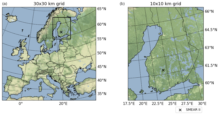
Figure 1 The two model domains: the European grid (a) with a cell size of $\sim \mathrm{30}\times \mathrm{30}$ km, and the nested grid (b) with a cell size of $\sim \mathrm{10}\times \mathrm{10}$ km (b). The black square on the European grid (a) indicates the position of the nesting. The black cross denotes the location of the SMEAR-II station.

Simulations were performed for the summer of 2019 (i.e., from 15 June to 31 August 2019) using two domains on a Lambert conformal projection: a first domain covering the whole of Europe at about 30×30 km resolution, and a second nested domain centered over Finland at about 10×10 km resolution (Fig. 1). The chemical mechanism used for the gas-phase chemistry was the MELCHIOR2 scheme (Derognat, 2003), including up to approximately 120 reactions with updated reaction rates (last updated in 2015). The ISORROPIA thermodynamic model was used to calculate the partitioning of the inorganic aerosol constituents (Nenes et al., 1998) and a logarithmic sectional distribution approach was deployed to treat the size distribution of aerosol particles using 15 bins ranging from 10 nm to 40 µm. The model additionally accounts for coagulation processes (Debry et al., 2007) as well as binary nucleation of sulfuric acid (H₂SO₄) and water (Kulmala et al., 1998). The treatment of OA in the model, and specifically of BSOA in the framework of the VBS scheme, is described in detail in the next section.

2.2 OA schemes

The VBS scheme was first implemented in the CHIMERE model for the Mexico City metropolitan area during the MILAGRO field experiment (Hodzic and Jimenez, 2011); however, the version included in the model is the one developed and applied over Europe for the Paris metropolitan area (Zhang et al., 2013). Oxidation products of BVOCs are distributed into four classes of volatility at saturation concentrations of 1, 10, 100, and 1000 µg m⁻³ (at 300 K) with different mass yields for low-NO_x and high-NO_x conditions based on the work of Hodzic and Jimenez (2011), and references therein, and allocated in a dedicated set to uniquely track their contribution to OA (Fig. 2). All monoterpene species have identical SOA yields but specific reactivities based on Bessagnet et al. (2008). The model employs a simplified treatment for the formation of BSOA from sesquiterpenes. BSOA from sesquiterpenes is considered only for the reaction against the ^⋅OH radical, and oxidation products distributed in the same volatility bins used for the rest of the BSOA precursors, and with no differentiation between low-NO_x and high-NO_x conditions. The reaction rate of sesquiterpenes (i.e., humulene lumped class) against OH is set to $\mathrm{2.9}\times {\mathrm{10}}^{-\mathrm{10}}$ molecule⁻¹ cm³ s⁻¹ with mass yields taken from Tsimpidi et al. (2010). The resulting gas-phase material can be further oxidized in the model by the ^⋅OH radical (curved blue arrows in Fig. 2) resulting in an increase of 7.5 % in the organic mass to mimic the addition of oxygen (Robinson et al., 2007) and in a simultaneous shift in volatility by 1 order of magnitude. In these VBS schemes, also referred to as “1D VBS schemes”, a fixed molecular structure, and therefore molecular weight, is assigned to each of the four volatility classes, i.e., 180 g mol⁻¹. The effective enthalpy of evaporation (ΔH_vap) of each BSOA volatility class is unique and set to 30 kJ mol⁻¹. The additional formation of BSOA from O₃ and NO₃ is taken into account following the same approach as Zhang et al. (2013). The complete list of the different SOA yields used in the model are reported in Table S1 in the Supplement.

Table 1 Reaction rate constants of BSOA aging as used in the different sensitivity tests. The schematic of the aging scheme is reported in Fig. 2.

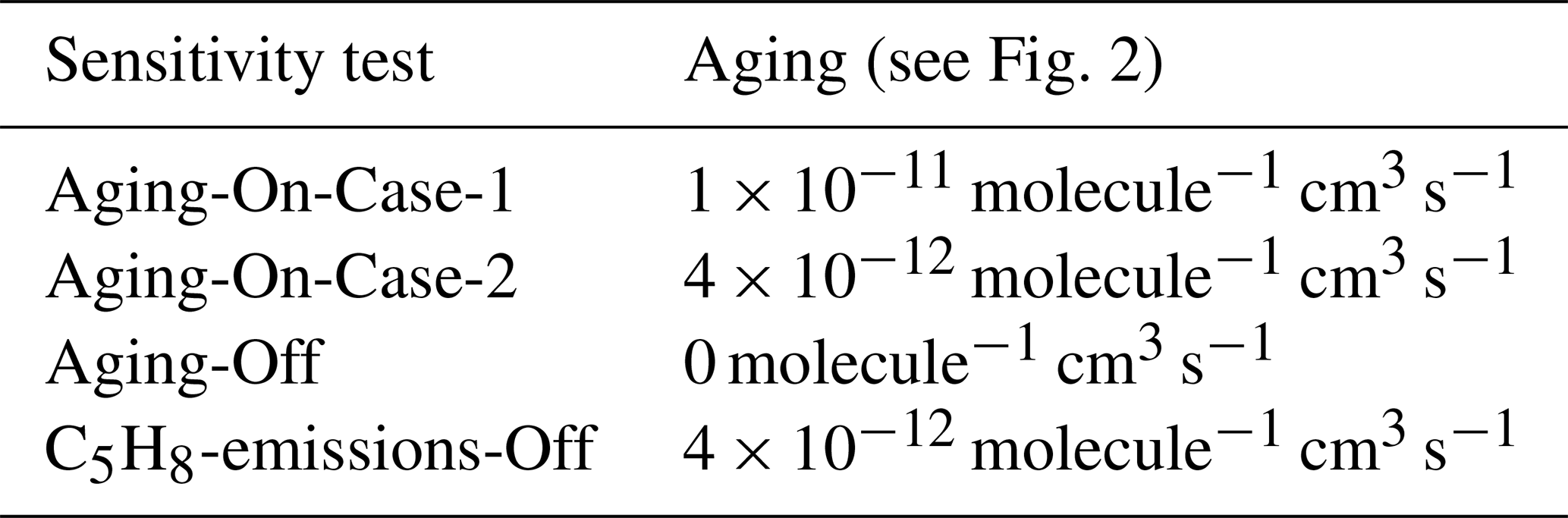
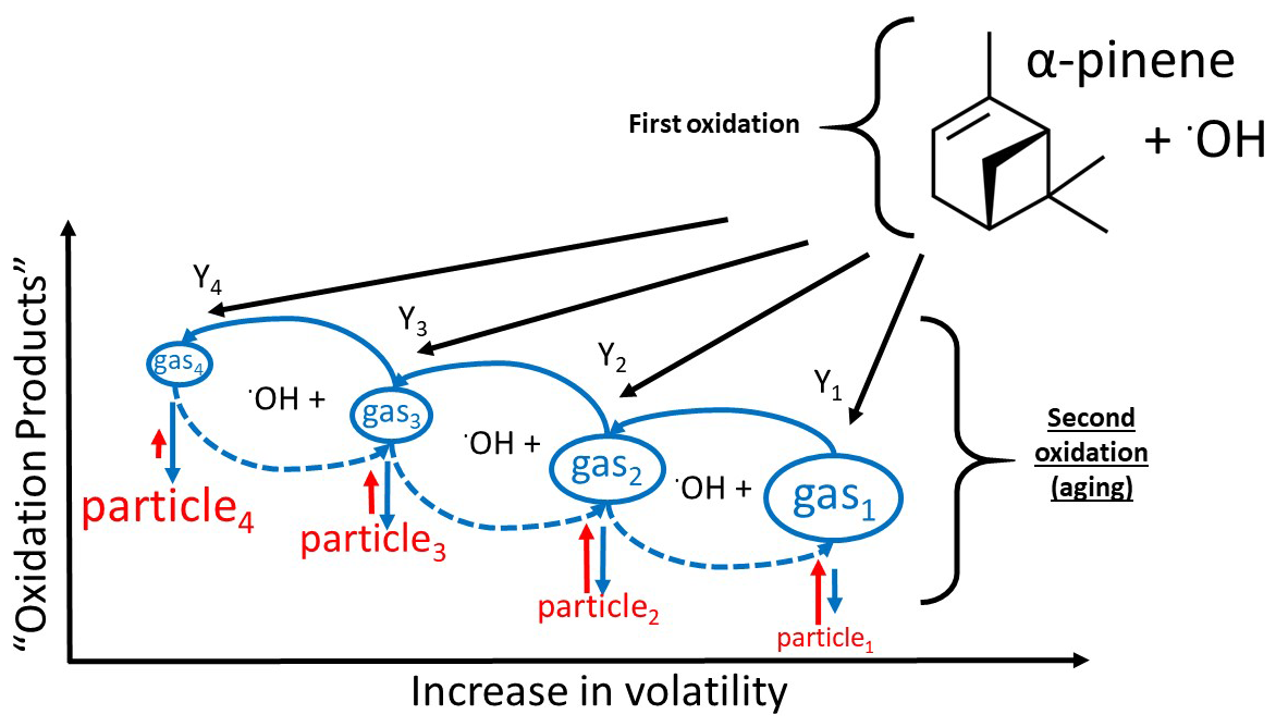
Figure 2 Schematic of the oxidation scheme of biogenic precursors as implemented in the VBS scheme of CHIMERE (here reported specifically for the C₁₀H₁₆ parent precursor). The black arrows represent the distribution kernel of the first oxidation products into the four volatility bins (Y₁… Y₄). The curved blue arrows represent the secondary oxidation processes, i.e., aging, along the four volatility bins, each of which decreases the volatility by 1 order of magnitude. The text font size represents the tendency of both particles and gas-phase organic material (OM) to transition in one or in the other phase (i.e., larger font size indicates a stronger affinity toward that phase, and vice versa). The dashed curved arrows represent the fragmentation process (also available in CHIMERE, but not currently used for this application).

Aging of biogenic aerosol has been tested in previous modeling applications at the European scale (Bergström et al., 2012; Cholakian et al., 2018; Zhang et al., 2013). However, very few of these studies have investigated the effects and impacts of using different biogenic aging schemes in an environment that is largely affected by biogenic emissions and by combining parallel state-of-the-art measurements of a vast array of atmospheric compounds. In this study, we performed a comprehensive evaluation of the different aging schemes as currently available from the literature. Specifically, we tested the oxidation of gas-phase biogenic organic material in the SVOC range, i.e., chemical aging, (curved blue arrows in Fig. 2). Additionally, we also tested the influence of isoprene emissions on BSOA formation (Table 1). In total, we performed four simulations, as described below:

• Aging-On-Case-1: gas-phase organic material of biogenic origin in the SVOC range can react with the ^⋅OH radical with a reaction rate of $\mathrm{1}\times {\mathrm{10}}^{-\mathrm{11}}$ molecule⁻¹ cm³ s⁻¹ (Murphy and Pandis, 2009; Zhang et al., 2013).

• Aging-On-Case-2: gas-phase organic material of biogenic origin in the SVOC range can react with the ^⋅OH radical with a reaction rate of $\mathrm{4}\times {\mathrm{10}}^{-\mathrm{12}}$ molecule⁻¹ cm³ s⁻¹ (Bergström et al., 2012; Lane et al., 2008). This simulation also represents the base-case simulation for the evaluation of both meteorological parameters and the photochemistry.

• Aging-Off: gas-phase organic material of biogenic origin in the SVOC range does not react further with the ^⋅OH radical. SVOC species are included in the partitioning equations and/or removed from the system via wet and/or dry deposition.

• C₅H₈-emissions-Off: emissions of C₅H₈ are inhibited in the emissions model (i.e., MEGAN). Gas-phase organic material of biogenic origin in the SVOC range can react with the ^⋅OH radical with a reaction rate of $\mathrm{4}\times {\mathrm{10}}^{-\mathrm{12}}$ molecule⁻¹ cm³ s⁻¹ (Bergström et al., 2012; Lane et al., 2008), i.e., based on Aging-On-Case-2.

Formation of ASOA is included by using the same range of volatilities as for BSOA. Aging of ASOA is accounted for in our application with a reaction rate of $\mathrm{1}\times {\mathrm{10}}^{-\mathrm{11}}$ molecule⁻¹ cm³ s⁻¹ (Murphy and Pandis, 2009; Zhang et al., 2013). This value is not altered across all the sensitivity tests. SVOCs arising from the evaporation of primary organic aerosols (POA) upon dilution are allowed to age with a reaction constant of $\mathrm{4}\times {\mathrm{10}}^{-\mathrm{11}}$ molecule⁻¹ cm³ s⁻¹ (Robinson et al., 2007) and no acid-enhanced BSOA production and anthropogenic pollution-enhanced SOA production is accounted for. No volatility dependence of Henry's law water solubility coefficients is included. The dry deposition of gases was treated with the Wesely scheme (Wesely, 1989).

2.3 Input data

Annual anthropogenic emissions of black carbon (BC), organic carbon (OC), carbon monoxide (CO), ammonia (NH₃), non-methane volatile organic compounds (NMVOCs), nitrogen oxides (NO_x), and sulfur dioxide (SO₂) were retrieved from CAMS for the whole year 2019 at 0.1×0.1^∘ resolution and distributed hourly over the periods investigated (summer of 2019) with temporal profiles based on the EMEP MSC-W model (Simpson et al., 2012). Biogenic emissions of NO, isoprene, limonene, α-pinene, β-pinene, ocimene, and humulene (representing the lumped class of sesquiterpenes) were prepared using the MEGAN model version 2.1 (Guenther et al., 2012). Emission rates of 15 plant functional types (PFTs), at an original horizontal resolution of $\mathrm{0.008}{}^{\circ }\times \mathrm{0.008}{}^{\circ }$, were re-gridded to match the resolution of both the coarse and high-resolution nested domains (i.e., 30 and 10 km, respectively). Standard emission rates are adjusted according to several environmental factors, based on local radiation and temperature values (among other variables such as leaf area index (LAI), Guenther et al., 2006). No emissions from wildfires were included in the simulations. Meteorological input was simulated with the WRF regional model (v3.71) (Skamarock et al., 2008) forced by the National Centers for Environmental Prediction (NCEP) Climate Forecast System Version 2 (http://www.ncep.noaa.gov, last access: 20 February 2023) with a temporal resolution of 6 h, a horizontal resolution of 1^∘, and with the course domain nudged toward the reanalysis data (every 6 h, i.e., surface grid nudging). Simulations were performed using the Rapid Radiative Transfer Model (RRTMG) radiation scheme (Mlawer et al., 1997), the Thompson aerosol-aware MP scheme to treat the microphysics (Hong et al., 2004), the Monin–Obukhov surface layer scheme (Janjic, 2003), and the NOAA Land Surface Model scheme for land surface physics (Chen and Dudhia, 2001).

Initial and boundary conditions of aerosols and gas-phase constituents were retrieved from the climatological simulations of LMDz-INCA3 (Hauglustaine et al., 2014), where a monthly average of several years is created on a global level and used as boundary conditions for the coarse domain, and from the Goddard Chemistry Aerosol Radiation and Transport (GOCART) model (Chin et al., 2002). For aerosol species the model includes inorganic species such as fine and coarse nitrate, ammonium, sulfate, dust, as well as OC and BC.

3 Observational data and model evaluation methods

Observational data were taken from at the SMEAR-II station located within the boreal forest of Finland (black cross in Fig. 1). Common meteorological parameters with a temporal resolution of 1 h were used to evaluate the performance of the WRF model, i.e., surface temperature, wind speed, wind direction, relative humidity, and precipitation.

The CHIMERE model was evaluated with gas-phase measurements of isoprene, monoterpenes, ozone, and nitrogen oxides (in dry air) taken at 4.2 m at a 1 h temporal resolution. Nitrogen oxide measurements were performed with a chemiluminescence analyzer (TEI 42 CTL), whereas ozone measurements were performed with an ultraviolet light absorption analyzer (TEI 49 C). Measurements of isoprene and monoterpenes BVOCs were performed via proton transfer reaction-mass spectrometry (PTR-MS, Rantala et al., 2015).

The modeled total organic aerosol mass (OA) was compared against aerosol chemical speciation monitor (ACSM) measurements available during the summer of 2019 (i.e., from 15 June to 31 August 2019). The ACSM measures the non-refractory (NR) sub-micrometer PM mass (i.e., material evaporating at 600^∘) with an aerodynamic diameter less than 1 µm (PM₁). A complete description of the ACSM measurements is available in Heikkinen et al. (2021). Finally, the modeled particle size distribution was compared against differential mobility particle sizer (DMPS) measurements.

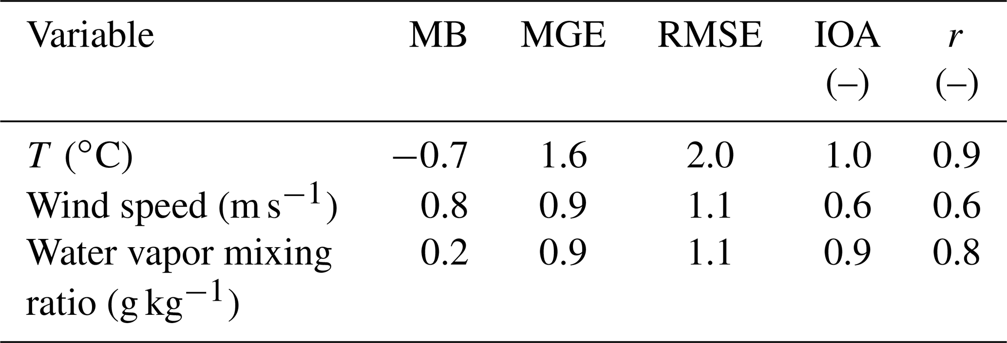
Table 2 Statistical metrics used for model evaluation. M_i and O_i stand for modeled and observed values, respectively, and N is the total number of paired values.

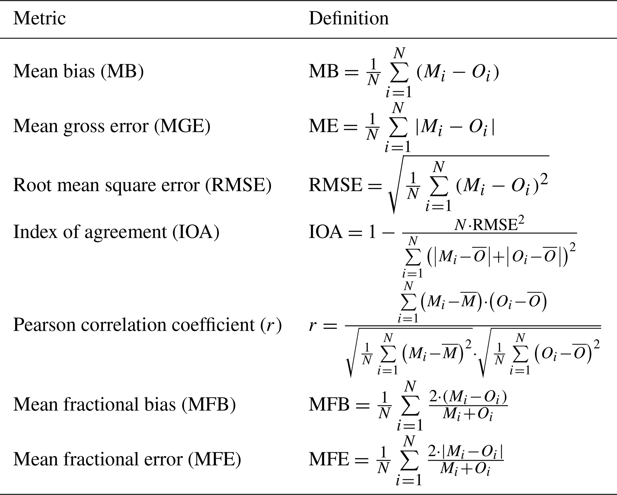
Additional measurements of OC and isoprene air concentrations were taken from the EBAS European database (https://ebas.nilu.no/, last access: 11 January 2024) (Tables S2 and S3). NO_x and O₃ measurements were retrieved for rural stations as available from the Air Quality e-Reporting (AQ e-Reporting) database (https://www.eea.europa.eu/en, last access: 11 January 2024). Specifically, 271 stations were retrieved for NO_x and 350 stations for O₃. Observations at these sites were compared against model data from the coarse grid (at 30 km). The statistical metrics used for the meteorological and chemical performance evaluation are reported in Table 2.

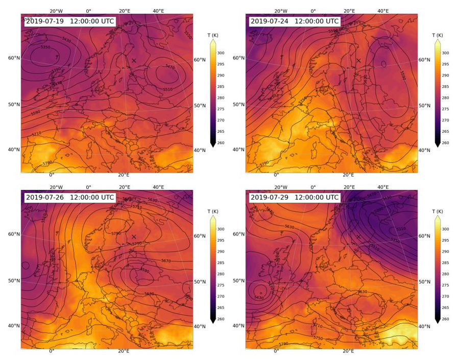
Figure 3 Geopotential height (m a.s.l.) at 500 hPa and air temperature (K) at 850 hPa for 4 d during the heat wave period (19–28 July 2019). Data are taken from the ERA5 reanalysis (available at https://cds.climate.copernicus.eu, last access: 11 January 2024). The black cross denotes the location of the SMEAR-II station.

4 Results

4.1 Synoptic context

The summer of 2019 was the second warmest on a global scale and was among the five warmest measured in Europe since the 16th century, producing a regional temperature anomaly close to 2 K (compared to 1981–2010), comparable to that of 2003 (Sousa et al., 2019). Two distinct severe heat wave events occurred during the period considered in this study, the first in late June and the second in late July. Both events were characterized by the presence of a low-pressure system in the northeastern Atlantic and a ridge extending over Europe, causing persistent anticyclonic conditions, low cloud cover, and warm sub-tropical air advection from northern Africa, a configuration typically associated with extreme temperatures (Tomczyk et al., 2017). The synoptic pattern of the late June heat wave was better defined, and affected mainly southwestern Europe, while the late July heat wave could reach further northward toward Scandinavia, affecting also Finland, where a record temperature of 33.2^∘ was measured on 28 July (Villiers, 2020). Besides the dynamical influence, the first event was enhanced by a vertical descent of potentially warmer air. By contrast, the late July heat wave was driven by diabatic fluxes and surface-atmosphere coupling, a process amplified by the soil moisture deficit produced by the first extreme event (Sousa et al., 2019). In Fig. 3 we show the large-scale configuration of the late July event, which strongly affected Finland. On 19 July the high pressure was already located on the Iberian Peninsula and started to expand northward. On 25 July the strongest pressure and temperature anomalies were registered in France and Spain, and the ridge started to influence northern Europe. After 26 July the Atlantic low moved east across Great Britain bringing cooler air to continental Europe, which was, however, still affecting Scandinavia. On 29 July Finland started to be influenced by western cold continental air.

4.2 Analysis and evaluation of meteorological parameters

Meteorological conditions are a fundamental ingredient in understanding the formation, transportation, and removal of pollutants (Bianchi et al., 2021; Seinfeld and Pandis, 2016). However, these are not always simultaneously analyzed in CTM applications, and often uncertainties are presented relative to the underlying gridded emissions and/or chemical mechanics. It is therefore important to also characterize the meteorological conditions and evaluate the key meteorological parameters that drive the physical and chemical processes.

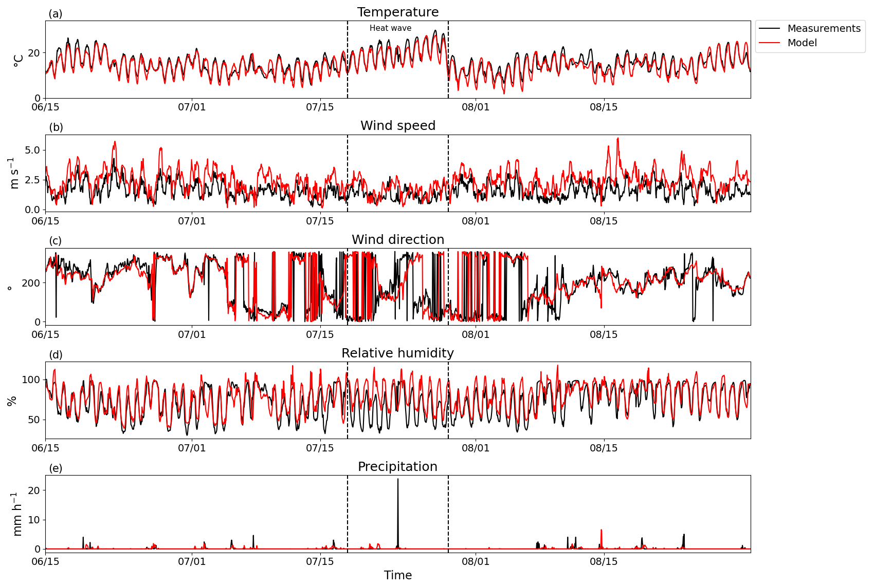
Figure 4 Hourly comparison of different meteorological parameters at the SMEAR-II station. From top to bottom: (a) temperature (^∘C), (b) wind speed (m s⁻¹), (c) wind direction (^∘), (d) relative humidity (%), and (e) precipitation (mm h⁻¹). Black lines indicate the measurement data and red lines the model data. The dashed lines delimit the periods with sustained elevated temperature, denoted here as “heat wave”.

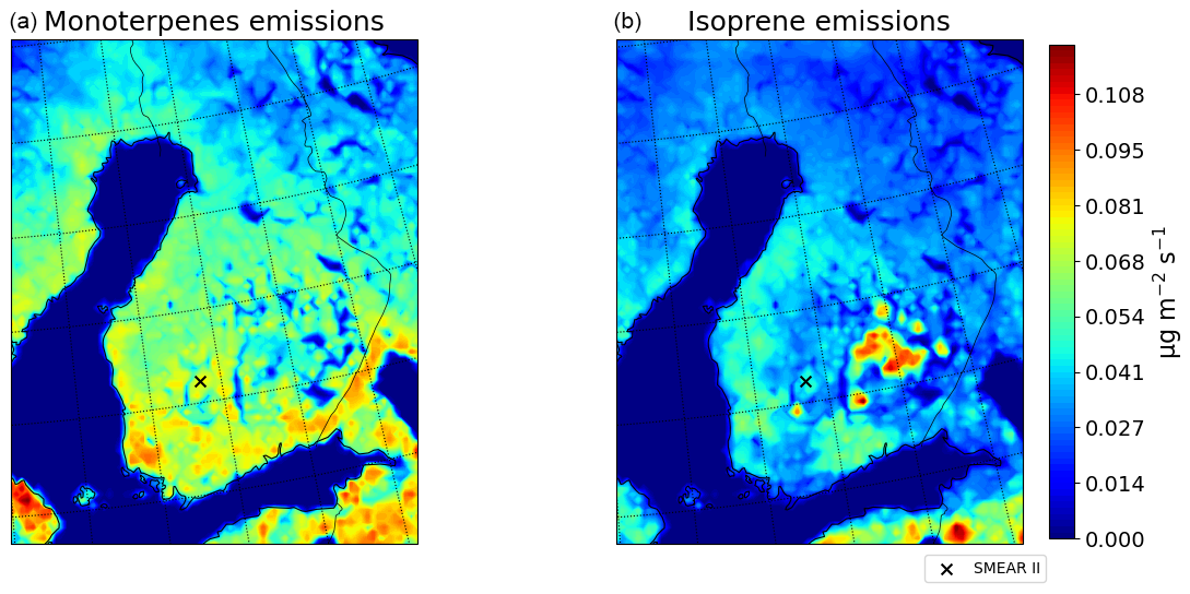
Figure 5 Average spatial distribution of monoterpene (a) and isoprene (b) emissions (µg m⁻² s⁻¹) for the summer of 2019 (15 June–30 August 2019). The cross denotes the location of the SMEAR-II station. Monoterpenes represent here the sum of all the available terpene species.

Figure 4 and Table 3 report the comparison between modeled and observed meteorological parameters at the SMEAR-II station. The site was characterized by rather warm temperatures during the very beginning of the simulations, which later transitioned into a colder period persisting until about 15 July. Afterward, a sustained increase in temperatures occurred between around 18 and 29 July (with daytime temperatures well above 20^∘) after which the temperatures dropped again until the end of the period. The model was able to reproduce such a temporal trend with a slight underestimation ($-\mathrm{0.7}{}^{\circ }$) occurring mainly during the nighttime periods (Fig. 4). A comparison between modeled and observed relative humidity also indicated a similar level of agreement with the diurnal variation captured well in the model, but some sporadic short-lived rain events were missed by the model.

Table 3 Model evaluation for the meteorological parameters (from 15 June to 30 August 2019). Statistical analysis performed at 1 h temporal resolution.

The analysis of the wind direction fields indicated that they were satisfactorily reproduced by the model, with the southern westerly (SW) sector being the most predominant wind direction during the summer period (r=0.5), but with wind speed generally over predicted. Quite low wind speed values (i.e., around 1–1.5 m s⁻¹) were observed during the middle of the simulation (from 18 to 29 July) concurrently with the “heat wave” episode, whereas values were generally higher (2–2.5 m s⁻¹) during the first half and second half of the investigated periods, a pattern that the model reproduced well (r=0.62).

4.3 Analysis of biogenic volatile organic compounds (BVOCs)

We report here the analysis of the biogenic emission fluxes (i.e., output from the MEGAN model) for emissions of monoterpenes, isoprene, and sesquiterpenes (humulene lumped class) as well as the comparison of their corresponding air concentrations (i.e., output from the CHIMERE model). Figure 5 shows the average spatial distribution of monoterpene and isoprene BVOCs for the investigated period and for the 10 km resolution nested domain centered over Finland. As expected, monoterpene emissions clearly dominate the biogenic emission flux over isoprene with a north-to-south gradient. The model indicated few localized areas, mainly in the eastern regions of the domain, where substantial isoprene emissions are evident. Specifically, at the location of the SMEAR-II station, isoprene emissions show a larger diurnal variability compared to monoterpenes (Fig. 6) with the model predicting up to about 59 %, 36 %, and 5 % of monoterpene, isoprene, and sesquiterpene (humulene) relative contributions to the total BVOC pool, respectively (Fig. 7).

Previous model estimations of biogenic emissions over the Finnish forest indicated that monoterpene emissions dominate the total BVOC pool, representing up to about 45 % of the annual total emissions, whereas isoprene emissions contribute about 7 % (Lindfors and Laurila, 2000), which is considerably lower than the isoprene relative contribution reported here. These discrepancies most likely arise from the different EFs, and land use types, that are used to retrieve the biogenic emission fluxes. Even though the underlying emission mechanism is very similar to the one used in previous studies (Guenther, 1997), the EFs applied to these early estimates of biogenic flux were specifically retrieved for boreal tree species, different from those used here, which are directly taken from measurements available in North America and Central Europe. Additionally, in the previous studies, tree species with no documented isoprene emission were assigned a minimum emission rate, whereas in this work we applied EFs as implemented in the MEGAN modeling framework (Guenther et al., 2006).

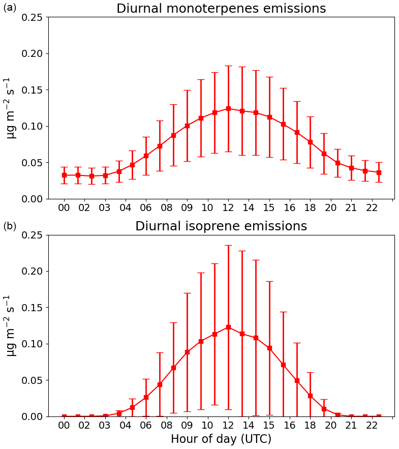
Figure 6 Average diurnal variation of monoterpene (a) and isoprene (b) emissions (µg m⁻²s) for the summer of 2019 (15 June–30 August 2019) at the SMEAR-II station. The extent of the red bars denotes 1 SD (1σ). Here, monoterpenes represent the sum of all the available terpene species.

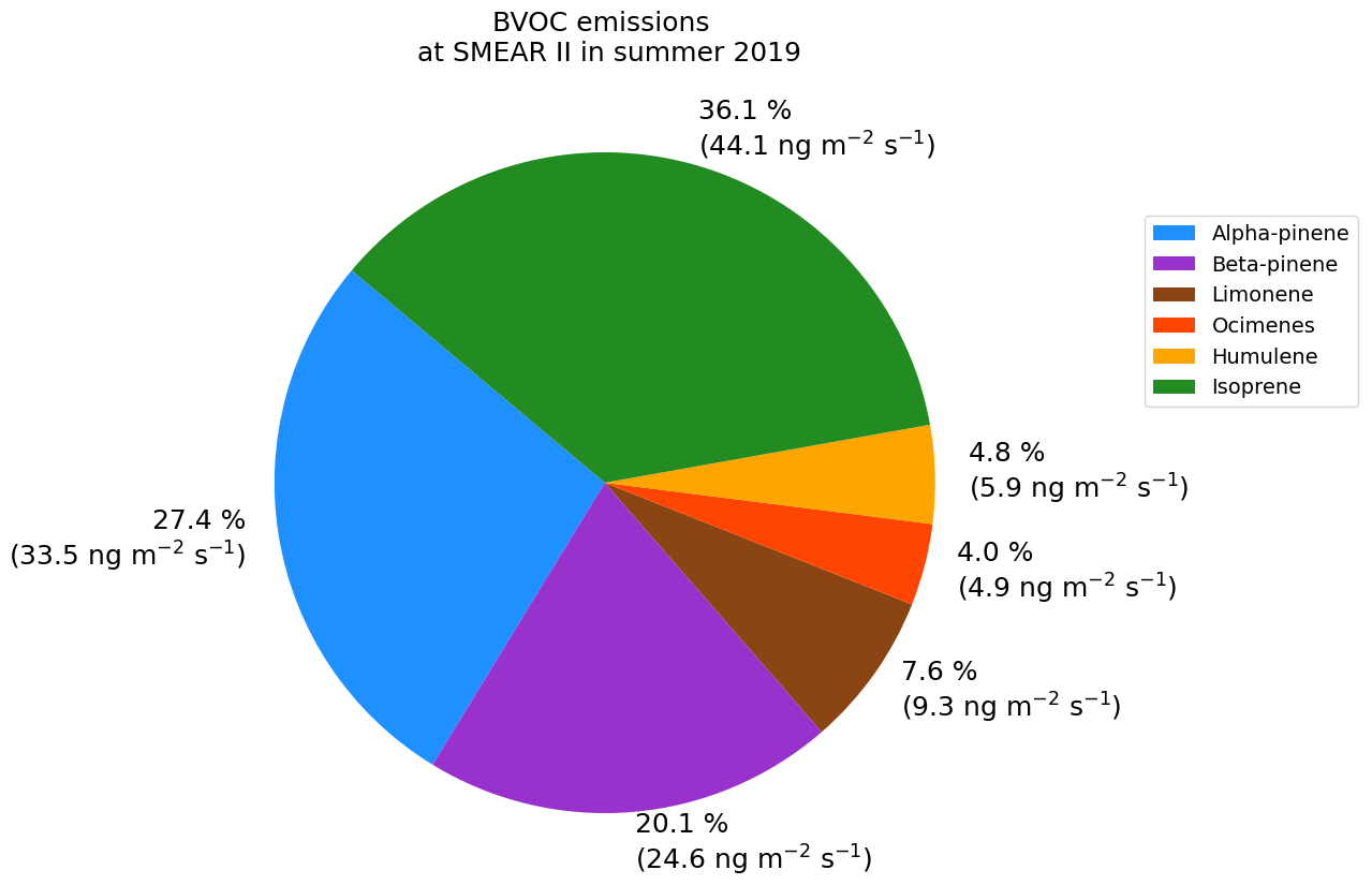
Figure 7 Average relative contribution of the BVOC species as predicted by the MEGAN model for the summer of 2019 (15 June–30 August 2019) at the SMEAR-II station. Units are in ng m⁻² s⁻¹.

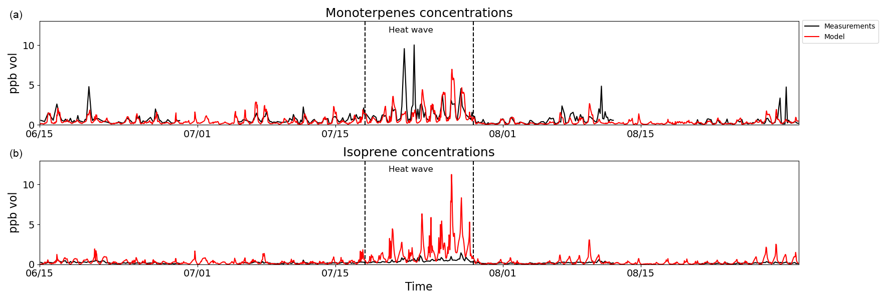
Figure 8 Hourly comparisons of model (red) and measured (black) air concentrations of (a) isoprene and (b) monoterpenes (sum of terpenes) at the SMEAR-II station. Units are in ppb vol. The dashed lines delimit the periods with sustained elevated temperature, denoted here as “heat wave”.

The comparison of isoprene and monoterpene air concentrations at the SMEAR-II station is reported in Fig. 8. The model could reproduce relatively well the concentrations of monoterpenes, with increasing values occurring during the warmer phases of the investigated period (denoted here as “heat wave”) and relative lower values during the colder periods (see Sect. 4.1). A few isolated spikes in monoterpene air concentrations are likely to arise from local anthropogenic activities in the nearby sawmill facilities (Heikkinen et al., 2021; Hellén et al., 2018; Vestenius et al., 2021), a feature that is not included in the emission model. Modeled sesquiterpene concentrations were found to be around 15 ppt on average for the investigated periods, which is comparable to the total detected sesquiterpene average concentrations reported by Hellén et al. (2018) for the summer of 2016. Isoprene concentrations also indicated an increase during periods characterized by warmer temperatures, but concentrations were largely overestimated. The ratio between the modeled and observed isoprene air concentration varies from 4 to 8, with a few isolated peaks exceeding a factor of 10 (Fig. 8). An additional comparison with isoprene air concentration data as available from the EBAS database indicated that the overestimation is systematic across most of the European sites (Fig. S1 in the Supplement). Specifically, the model shows an overestimation of isoprene at 70 % of the stations analyzed. It is interesting to note that also for the additional station located in Finland, i.e., Pallas (FI0096G), the model showed a substantial overprediction of isoprene emissions (Fig. S1), therefore indicating that the problem might be more accentuated for European boreal forests. This is also confirmed by a very recent global modeling study presented by Zhao et al. (2023) where the GEOS-CHEM model was applied over the northern high latitudes (Zhao et al., 2023). Overestimations of isoprene in CTM applications with the MEGAN model at the SMEAR-II site were also reported in the study by Jiang et al. (2019a), which used the Comprehensive Air Quality Model with Extensions (CAMx) to simulate the entire year of 2011, and, more recently, in a WRF-CHIMERE application over the pine forest in southwestern France (Cholakian et al., 2023). Although the models use different chemical schemes to perform the gas phase and particle phase chemistry, they both indicated a large overestimation of isoprene concentrations, also at other European sites. The implications of such an overestimation in isoprene biogenic emissions are analyzed in detail in Sect. 4.5.

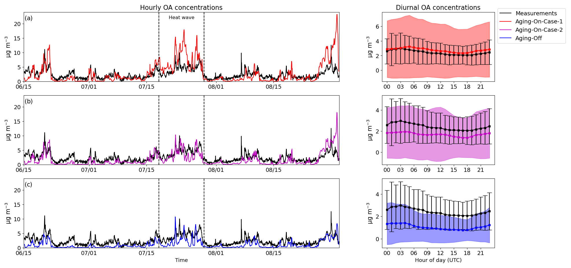
Figure 9 Model (different colors) and measured (black) air concentrations of OA for the (a) Aging-On-Case-1, (b) Aging-On-Case-2, and (c) Aging-Off BSOA schemes. Hourly (left) and diurnal (right) comparisons at the SMEAR-II station. The dashed lines delimit the periods with sustained elevated temperature, denoted here as “heat wave”. The extent of the bars and the shaded areas denotes 1 SD (1σ). Units are in µg m⁻³.

4.4 Analysis and source apportionment of OA

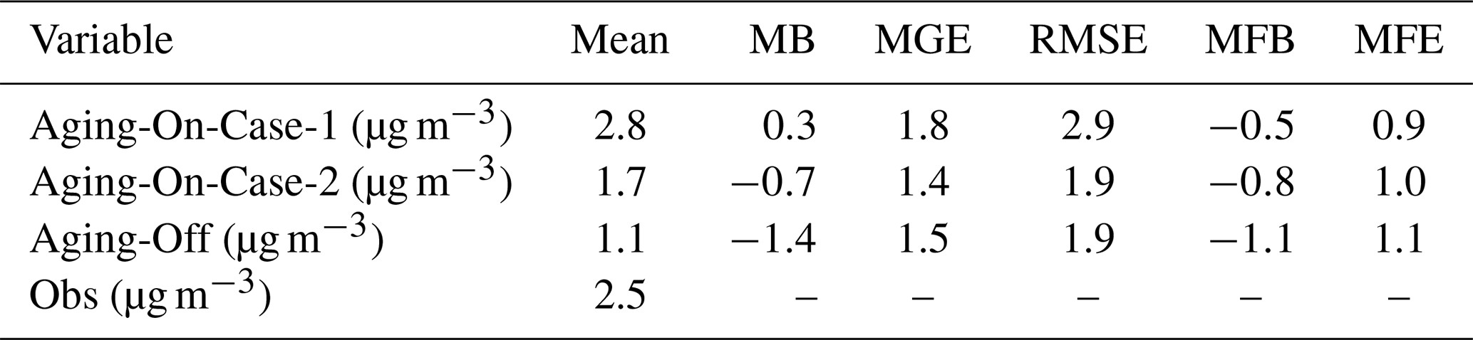
The modeled total OA fraction is compared against OA measurements performed with the ACSM instrumentation (Heikkinen et al., 2021). In the model, this fraction represents the sum of POA (i.e., primary emitted organic material) and SOA (i.e., secondary formed organic material upon oxidation and subsequently condensation of the resulting low-volatile vapors) from all the sources considered in the simulation (biogenic, anthropogenic, as well as boundary conditions). Figure 9 reports the hourly and diurnal comparisons for all three BSOA schemes under evaluation. Specifically, the model can reproduce the temporal trends of the observed OA fraction relatively well: the three main peaks occurring during the beginning, the “heat wave”, and the last week of the investigated periods are all captured, but their magnitude depends greatly on the specific BSOA scheme (Table 1). We additionally compared model data against organic carbon (OC) measurements available from 15 additional EBAS sites (Table S2) and at different temporal resolutions (from 4 h to 1 week). Since the model uses the organic aerosol (OA) mass concentration in its own calculations, we applied the $\mathrm{OM}/\mathrm{OC}$ ratio of 1.7 as representative for BSOA (Bergström et al., 2012). Results indicated similar behaviors also for OC data (Fig. 10), with the model showing a substantial increase in the OC mass and with a larger overestimation for aging schemes that account for very aggressive aging processes. The mean bias varies from 0.63, −0.13 and −1.1 for the Aging-On-Case1, Aging-On-Case2, and Aging-off case, respectively (Table S4).

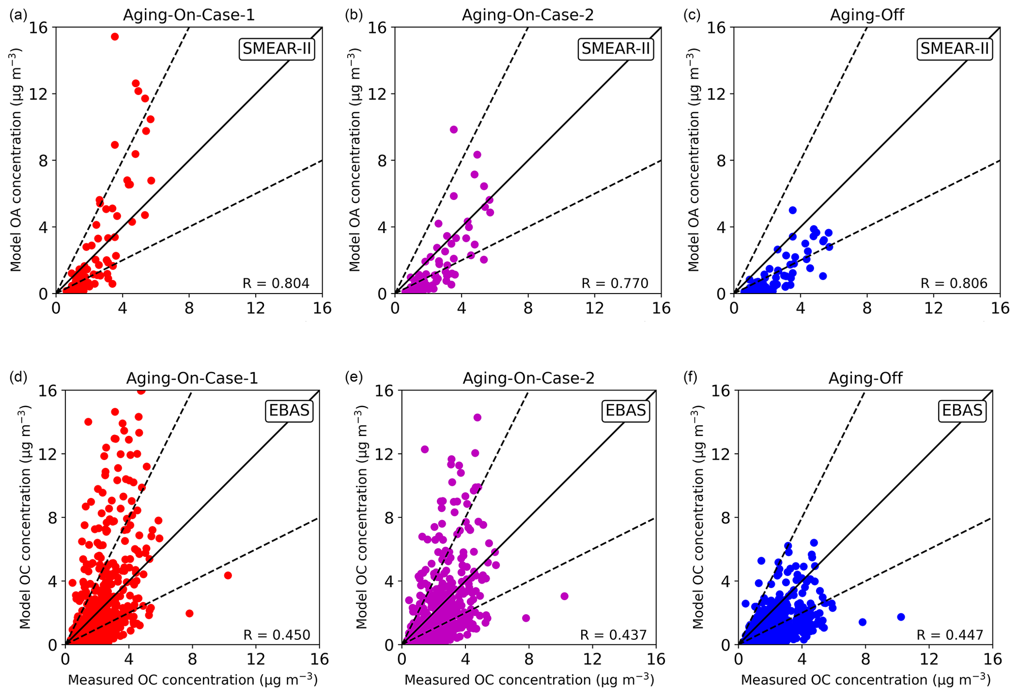
Figure 10 Model (y axis) and measured (x axis) air concentrations of OA for the Aging-On-Case-1 (a, d), (b) Aging-On-Case-2 (b, e), and (c) Aging-Off (c, f) BSOA schemes at the SMEAR-II station (a, b, c, daily averages) and OC at available EBAS sites (d, e, f). Solid line indicates the 1:1 line. The dashed lines delimit the 1:2 and 2:1 lines. Units are in µg m⁻³. Data from the EBAS database have a temporal resolution varying from 4 h to 1 week, depending on the specific site.

Additionally, periods with relatively low concentrations are also well reproduced, with no substantial positive bias observable. The analysis of the diurnal profiles indicates that the model can reproduce the daily variation, with a rather flat diurnal variation of OA concentrations which increase slightly during nighttime and early morning hours. The model tends to underestimate OA at Hyytiälä, especially during periods with low measured concentrations (Fig. 9). This might suggest uncertainties in the background OA fields used in the model and/or in the concentrations injected at the very boundaries of the coarser domain (i.e., long-range transport).

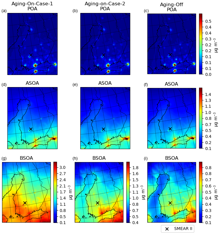
Figure 11 POA (a, b, c), ASOA (d, e, f), and BSOA (g, h, i) average concentrations during the summer of 2019 (15 June–30 August 2019) and for the Aging-On-Case-1 (a, d, g), Aging-On-Case-2 (b, e, h), and Aging-Off (c, f, i) BSOA schemes. The cross denotes the location of the SMEAR-II station. Units are in µg m⁻³. A different scale is used for the BSOA panel (g, h, i) to facilitate comprehension of the panel.

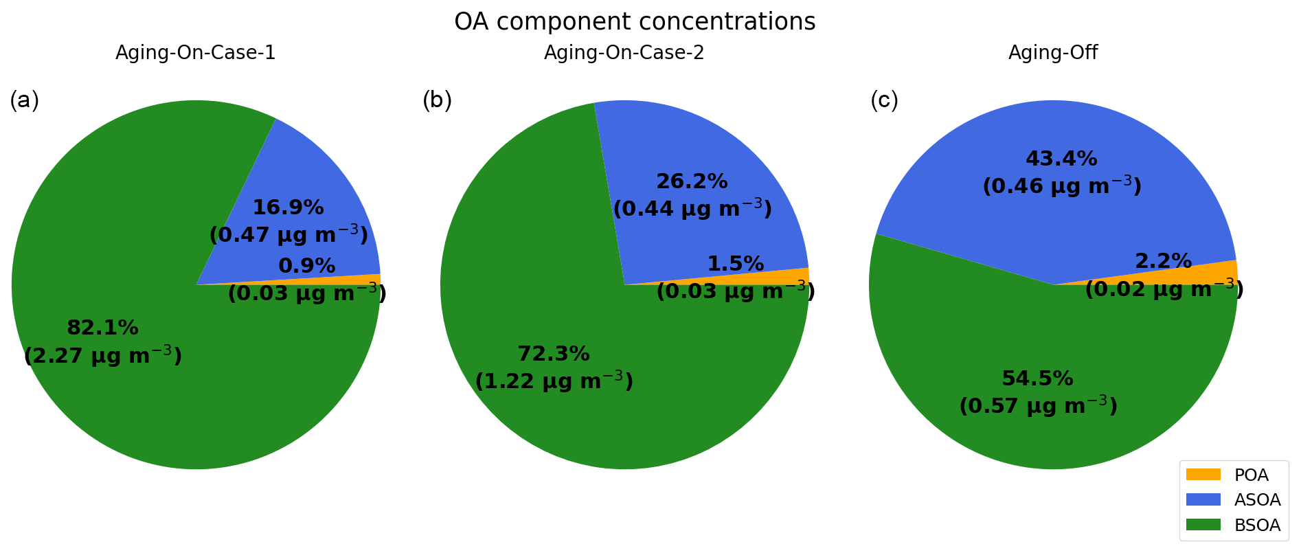
Figure 12 POA (orange), ASOA (blue), and BSOA (green) modeled average relative contribution to the total OA fraction for the summer of 2019 (15 June–30 August 2019) and for the Aging-On-Case-1 (left), (b) Aging-On-Case-2 (center), and (c) Aging-Off (right) BSOA schemes at the SMEAR-II site. Absolute concentrations are reported along with their relative contribution to the total OA.

The model-based source apportionment of the OA fraction for the three different BSOA schemes is reported in Figs. 11 and 12 for the entire domain as well as for the SMEAR II station. As expected, not much of a difference is noticed for the POA and anthropogenic secondary organic aerosol (ASOA) concentration for the different aging schemes, with POA contributing largely over the urban areas of Helsinki, Turku, and over Tallinn and Saint Petersburg, with average concentrations up to about 0.5 µg m⁻³. The model-based source apportionment predicted ASOA concentrations to exceed POA ones, sometimes also in urban areas, as, for example, over the urban area of Helsinki, and in general in the southern part of the domain where concentrations are relatively higher compared to northern regions (up to about 1.5 µg m⁻³). BSOA concentrations, on the other hand, were predicted to be more heterogeneously distributed within the domain (inner domain), and the OA mass increases significantly as aging processes are increasingly accounted for. For instance, in the Aging-Off scenarios, concentrations reach a maximum of around 1 µg m⁻³ on average over the whole period, whereas in the Aging-On-Case-1 scenario they reach up to 3 µg m⁻³ on average. This represents a substantial difference in the modeled BSOA mass, which is mainly driven by periods characterized by higher temperatures and therefore higher photochemical activity (Fig. 9).

Table 4 Model evaluation for the BVOC species isoprene and monoterpenes at the SMEAR II station (from 15 June to 30 August 2019). Statistical analysis performed at 1 h temporal resolution.

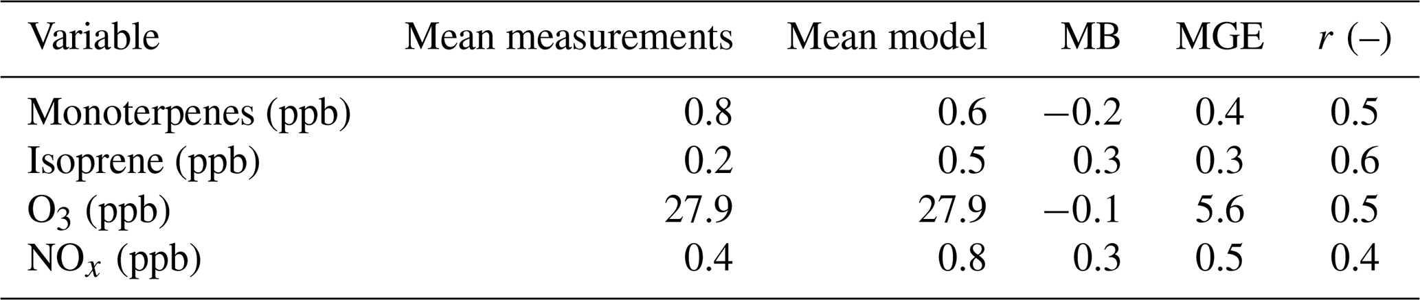
Table 5 Model evaluation for OA as predicted by the three BSOA schemes at the SMEAR II station (from 15 June to 30 August 2019). Statistical analysis performed at 1 h temporal resolution.

The pie chart in Fig. 12 reports the modeled average relative contribution of the OA fraction at the SMEAR-II site. Each of the three parameterizations indicated that the secondary fraction of OA is the dominant one, which is also in agreement with the positive matrix factorization (PMF) analysis performed on the ACSM data (Heikkinen et al., 2021). In the latter, a statistical source apportionment study of the OA measurement data was performed using the spectral profiles from the ACSM. The authors were able to identify three categories of OA: low-volatility oxygenated OA (LV-OOA), semi-volatile oxygenated OA (SV-OOA), and primary OA (POA). Their results indicated that LV-OOA and SV-OOA almost accounted for the entire OA mass during the summer periods (and eventually also during winter periods), with LV-OOA being the dominant component throughout the entire year. On the other hand, the highest SV-OOA contribution to the OA mass was identified during summer periods (about 40 %), with a distinct diurnal cycle with peaks in the early morning and in the late evening (in line with the diurnal profiles indicated by WRF-CHIMERE, Fig. 9). Nevertheless, a comparison of the PMF-retrieved SV-OOA and LV-OOA components against WRF-CHIMERE data is currently challenging because of the limited number of volatility bins used in the model to describe the formation of BSOA (i.e., currently limited to 4 at 1, 10, 100, and 1000 µg m⁻³ at 300 K), which only partially cover the low-volatility range (Bianchi et al., 2019). This limitation was further investigated by comparing the model size distribution with DMPS measurements at the SMEAR-II site. The model largely overestimates the number of particles below 100 nm and underestimates the accumulation mode (Fig. S2). This behavior was already reported in the work of Tuccella et al. (2019), who used aircraft measurement data (available both in the PBL and in the free troposphere) to evaluate the model size distribution. If we acknowledge that this model version does not account for any adjustment of the organic compounds based on their size, i.e., Kelvin effect (which will reduce the amount of semi-volatile compounds condensing on very small particles, mainly below 10 nm in size), and that the number of particles is retrieved in a prognostic manner from the total OA mass, density, and particle diameter, it is likely that the lack of a more explicit representation of the LVOC and ELVOC compounds (i.e., volatility bins) in this VBS framework (Fig. 2) could potentially reduce the growth, by condensation, of particles in the lower end of the size distribution, therefore adding to the overestimation of the smaller diameters and to the under-prediction of the larger ones (which will additionally reduce the coagulation efficiency of smaller particles toward larger sizes).

Finally, the model-based relative contribution of ASOA and BSOA to the total OA mass indicates substantial variations depending on the chemical scheme adopted. For the Aging-Off test the model predicted up to 43 % contribution of the anthropogenic SOA fraction to the total OA mass, which is very likely overestimated for the SMEAR-II boreal site. The aging of BSOA yield results that are more reasonable both in terms of the contribution of the single OA components and also in terms of the absolute concentrations (for the Aging-On-Case-2 BSOA scheme), i.e., with the BSOA fraction contributing up to 72 % to the total OA and the total OA mass negatively biased by 0.7 µg m⁻³ (Table 5).

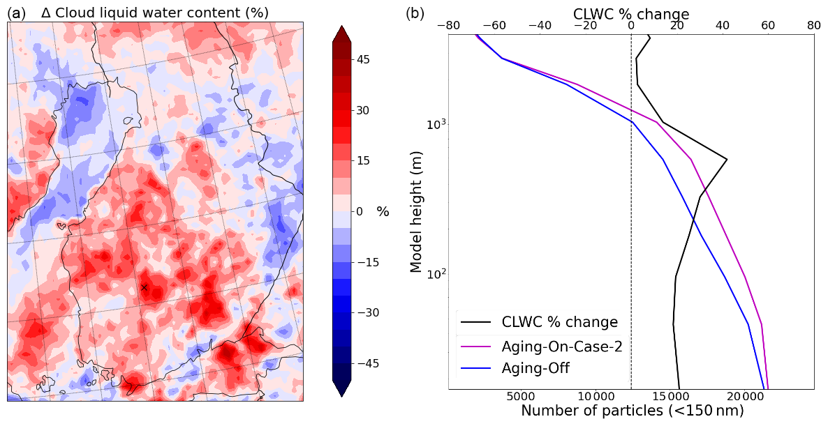
Figure 13 Integrated (vertical) differences in cloud liquid water content (left) over the high-resolution domain (10 km). Vertical profile of particles below 150 nm in the Aging-On-Case-2 and Aging-Off simulations and of the relative changes in cloud liquid water content (right) over the SMEAR-II site (average of a 3×3 km cell). The relative changes are reported here as ((Aging-On-Case-2 – Aging-Off)/Aging-Off) ×100.

4.5 Impacts on cloud liquid water content (clwc)

We report the preliminary analysis for the changes in modeled cloud liquid water content (clwc) between the different aging schemes. As discussed in Sect. 2.1, we run the model in an “online” configuration, therefore allowing CHIMERE to pass the diagnosed particle size number distribution, aerosol bulk hygroscopicity, ice nuclei (IN), and deliquesced aerosol to the WRF model. CHIMERE chemical and physical parameters were passed to the WRF model with an exchange frequency of 20 min and the aerosol activation to cloud droplets treated with the Abdul-Razzak and Ghan scheme (Abdul-Razzak, 2002) using a similar approach available in the WRF-Chem model (Chapman et al., 2009). More details on the aerosol–cloud interaction in WRF-CHIMERE can be found in Tuccella et al. (2019).

Figure 13 reports the vertically integrated average relative changes in clwc between the Aging-On-Case-2 and Aging-Off schemes for the entire simulation period. We calculated these differences using the Aging-On-Case-2 scenario since it yields the best results against OA measurements (Sect. 4.3). We report the vertical distribution of aerosol particles up to 150 nm, i.e., including particles that can effectively act as cloud condensation nuclei (CCN), as in the Aging-On-Case-2 and Aging-Off scenarios. Generally, the model indicated an increase in the clwc when the aging of biogenic aerosols is accounted for, owing to the increase in the biogenic aerosol mass loading (Fig. 10) and therefore of the number of biogenic particles that can act as CCN (Fig. S2). Changes in clwc are predicted to be larger over the land, and especially in the central region of the domain and over the SMEAR-II site where the model indicates around 30 % increase in clwc in the Aging-On-Case-2 with respect to the Aging-Off scenario. Most of the changes, i.e., total number of particles up to 150 nm and clwc, occurred below about 1000 m above sea level (a.s.l). which is roughly the estimated average PBL height during the summer period at SMEAR-II (Sinclair et al., 2022), with larger increases, in both particle number and clwc, slightly below the 1000 m a.s.l. altitude. Climatic feedbacks from biogenic particles over boreal areas were very recently reported by Yli-Juuti et al. (2021) using remote sensing and ACSM observations available at the SMEAR-II stations. Specifically, the analysis indicated an increase in OA loading, and CCN, during the 2012–2018 period as results of the increase in surface temperature. Higher cloud optical depth data were also statistically significantly associated with higher OA loading, providing direct evidence for the indirect effect of biogenic aerosols. The model results presented here seem to be in line with such results, but a separate study is needed to analyze in greater detail the modeled indirect effect under longer periods of time (i.e., model trend analysis).

4.6 Sensitivity of BSOA formation to C₅H₈ emissions

In this section we discuss the sensitivity analysis with inhibited isoprene biogenic emissions. As presented in the previous section, modeled isoprene air concentrations were largely overestimated at the SMEAR-II site (most likely because of the overstated isoprene emissions) and especially during periods characterized by high temperatures and intensive photochemical activity (referred to as “heat wave” episodes). Particle mass yield from isoprene biogenic compounds is lower compared to monoterpenes, and recent studies have shown that isoprene can effectively scavenge ^⋅OH radicals, preventing their reaction against other terpenoids and therefore limiting the formation of biogenic aerosol particles and the total organic mass (McFiggans et al., 2019).

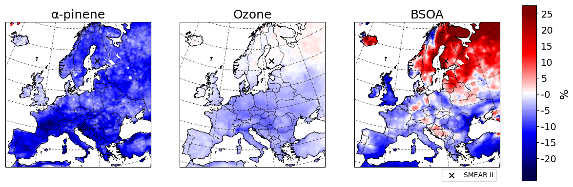
Figure 14 Daytime average (08:00–20:00 LT) relative changes in C₁₀H₁₆ (alpha-pinene) air concentrations, ozone, and BSOA concentrations with and without isoprene emissions. The relative changes are calculated as ((C₅H₈-emissions-Off – Aging-On-Case-2)/Aging-On-Case-2) ×100.

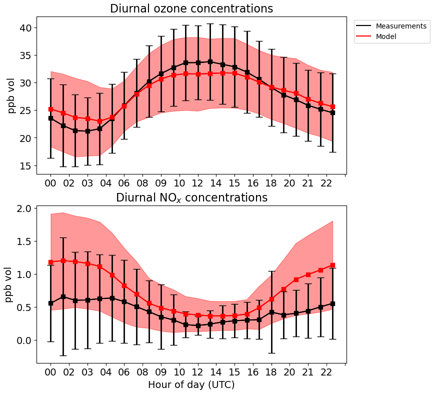
Figure 15 Diurnal variation of O₃ and NO_x at the SMEAR-II site (from 15 June to 30 August 2019). The extent of the bars and the shaded areas denotes 1 SD (1σ). Measurement data are shown in black and model data in red. Units are in ppb vol.

Figure 14 reports the daytime relative changes in α-pinene, O₃, and BSOA concentrations between the two simulations performed with and without isoprene emissions across all of Europe. Inhibiting isoprene emissions resulted in a non-negligible increase in the BSOA mass concentrations over larger areas of the northern part of the domain. In most of the areas, the BSOA mass increased by about 10 % with maximum increases at around 25 %. Conversely, α-pinene air concentrations were homogenously reduced all over the domain (Fig. 14). The relative reductions (over land) were on the order of 10 %–20 %. As isoprene emissions are excluded from the modeling system, more α-pinene of biogenic origin can effectively react with available radicals, i.e., ^⋅OH radicals, and, owing to its higher mass yield compared to isoprene, effectively increase the production efficiency of BSOA. This process is most likely favored by the large pool of α-pinene emissions available over the boreal forest regions (and by the lower temperatures compared to continental and southern Europe) which favors the transition of oxidized gases in the particle phase. Figure 14 also reports the relative changes in O₃ concentrations between the two simulations performed with and without isoprene emissions which were predicted to be very mild over northern Europe and larger over continental and southern Europe because of enhanced photochemical activities and large availability of isoprene emissions in the southern regions of the domain. The formation of O₃ is driven by the availability of both NO_x and VOC emissions, with the study area, SMEAR-II, clearly belonging to an NO_x-limited regime. As reported in Fig. 15, the model is able to reproduce the diurnal variation and absolute values (ppb) of O₃ very well (mean bias of −0.1 and 0.3 ppb for O₃ and NO_x, respectively, Table 4), whereas NOx concentrations were overestimated during nighttime periods, a behavior that was also confirmed by an additional evaluation against NO_x and O₃ measurements retrieved across the whole of Europe from the Air Quality e-Reporting database (https://www.eea.europa.eu/en, last access: 11 January 2024) (Fig. S3 and Table S5). Additionally, both the model and measurement data did not show a substantial local production of O₃ concentrations, i.e., both model and observational O₃ values increased from about 25 to about 30 ppb. This suggests that a large fraction of the O₃ measured at the SMEAR-II site is of long-range origin, therefore explaining the relative low changes in its concentrations between the two scenarios in the northern regions, as also reported by previous studies (Curci et al., 2009).

5 Conclusions

We presented a modeling evaluation study aimed at evaluating the formation of biogenic secondary organic aerosol (BSOA) over the Finnish boreal forest with the WRF-CHIMEREv2020r2 model. We investigated the formation of BSOA using different aging schemes to treat the second-generation oxidation product of BSOA, also referred to as “chemical aging”, currently available from the literature. Results were evaluated against high-resolution organic aerosol (OA) measurements performed with an aerosol chemical speciation monitor (ACSM) at the SMEAR-II site, an area largely affected by biogenic emissions. We used parallel measurements of biogenic gas-phase precursors (i.e., isoprene and monoterpenes) to investigate the model performance with respect to the BSOA precursors, which offers a proper framework with which to evaluate chemical transport model (CTM) simulations with a greater level of details. Additionally, we evaluated the response of the model to changes in isoprene emissions and the impact of different chemical schemes on the predicted cloud liquid water content (clwc).

The meteorological evaluation of standard parameters affecting the formation and transportation of BSOA was found to be satisfactorily reproduced throughout the whole simulated period, underlying the capability of the WRF model to properly reproduce the meteorological regimes of the summer of 2019 at a 10 km grid resolution.

The model was able to reproduce the diurnal variation of the OA mass well, as measured at the SMEAR-II site. As expected, BSOA aging processes significantly increased the BSOA mass, yielding reasonable model performance, both in terms of the total OA mass as well as in terms of source contribution (i.e., POA, ASOA and BSOA), for schemes that account for BSOA aging as proposed in a previous study (Bergström et al., 2012). On the other hand, the analysis of the model size distribution indicated a large overestimation for particles below about 100 nm and an underestimation for particles in the larger diameter sizes. We attributed such compensating effect to (1) a lack of an explicit treatment of organic compounds in the LVOC and ELVOC range, which can effectively condense on smaller particles and promote their growth to larger particle sizes, and to a lesser extent (2) to the lack of the Kelvin effect in the model calculation. Overall, these results stressed once more the need to properly represent the volatility distribution in CTM applications, and more work is needed in this direction, particularly on the volatility distribution of BSOA and on the implementation of physical processes affecting the evolution of the size distribution (e.g., inclusion of organic gases in the very low volatility ranges).

Additionally, the analysis of biogenic gas-phase precursors indicated that the model largely overestimated isoprene emissions, most likely because of overstated emissions in the MEGAN emission model, as already presented in various applications of the MEGAN model at the European scale. There is still a need to further reduce the uncertainties in the current estimation of biogenic fluxes (especially at northern latitudes), as one of the key parameters influencing the formation of BSOA in CTMs. An additional sensitivity test indicated that an overestimation could potentially reduce the production of BSOA by scavenging ^⋅OH radicals that would have been available to react against α-pinene compounds which have higher SOA yields.

Finally, our model results indicated an increase in the clwc when aging of BSOA is accounted for, most likely because of the increased number of aerosol particles acting as cloud condensation nuclei (CCN), as recently also suggested by measurement studies conducted at the SMEAR-II site. These preliminary results reported here should be corroborated with a more detailed modeling study spanning multiple years (i.e., trend analysis).

Overall, the model evaluation presented here indicated once more the importance of properly characterizing both biogenic emission fluxes and chemical scheme parameterization in order to correctly predict the formation of BSOA and its size distribution. As the climate continues to warm, biogenic emissions could become an increasingly important contributor to the total OA pool, and model predictions could vary significantly depending, also, on the level of confidence of the emission strength and chemical parameterization.