the Creative Commons Attribution 4.0 License.
the Creative Commons Attribution 4.0 License.
 | 16 Jul 2024
Using deep learning to integrate paleoclimate and global biogeochemistry over the Phanerozoic Eon
Dongyu Zheng
Andrew S. Merdith
Yves Goddéris
Yannick Donnadieu
Khushboo Gurung
Benjamin J. W. Mills
Databases of 3D paleoclimate model simulations are increasingly used within global biogeochemical models for the Phanerozoic Eon. This improves the accuracy of the surface processes within the biogeochemical models, but the approach is limited by the availability of large numbers of paleoclimate simulations at different pCO2 levels and for different continental configurations. In this paper we apply the Frame Interpolation for Large Motion (FILM) deep learning method to a set of Phanerozoic paleoclimate model simulations to upscale their time resolution from one model run every ∼25 million years to one model run every 1 million years (Myr).
Testing the method on a 5 Myr time-resolution set of continental configurations and paleoclimates confirms the accuracy of our approach when reconstructing intermediate frames from configurations separated by up to 40 Myr. We then apply the method to upscale the paleoclimate data structure in the SCION climate-biogeochemical model. The interpolated surface temperature and runoff are reasonable and present a logical progression between the original key frames.
When updated to use the high-time-resolution climate data structure, the SCION model predicts climate shifts that were not present in the original model outputs due to its previous use of widely spaced datasets and simple linear interpolation. We conclude that a time resolution of ∼10 Myr in Phanerozoic paleoclimate simulations is likely sufficient for investigating the long-term carbon cycle and that deep learning methods may be critical in attaining this time resolution at reasonable computational expense, as well as for developing new fully continuous methods in which 3D continental processes are able to translate over a moving continental surface in deep time. However, the efficacy of deep learning methods in interpolating runoff data, compared to that of paleogeography and temperature, is diminished by the heterogeneous distribution of runoff. Consequently, interpolated climates must be confirmed by running a paleoclimate model if scientific conclusions are to be based directly on them.
- Article
(10965 KB) - Full-text XML
- BibTeX
- EndNote


To simulate global environmental change over Phanerozoic time, it is important to understand how continental surface processes operate. For example, the weathering of silicate minerals controls the removal of atmospheric CO2, and phosphorus input from weathering plays a major role in the long-term oxygenation of the Earth (Walker et al., 1981; Lenton and Watson, 2004). Weathering rates are largely controlled by local erosion rates, temperature, and hydrology (West, 2012; Maher and Chamberlain, 2014), and the latest generation of Phanerozoic global biogeochemical models aim to represent these factors at the local scale using data from 3D general circulation model (GCM) simulations (Goddéris et al., 2023). Due to the long computational timescales of GCMs (typically weeks to months per ∼5000-year simulation for a fully coupled ocean–atmosphere model), they cannot be run interactively with long-term biogeochemical cycles over millions of years. Therefore, the “spatialized” deep-time biogeochemical models such as GEOCLIM (Donnadieu et al., 2006; Goddéris et al., 2014) and SCION (Mills et al., 2021; Longman et al., 2022) rely on either discrete time intervals or linear interpolation between times set by previously computed climate model simulations.
Currently both the GEOCLIM and the SCION models use a set of 22 continental configurations (including the present day) whose climate has been simulated by the Fast Ocean Atmosphere Model (FOAM) at a range of different CO2 levels. This equates to one set of model runs every ∼25 million years on average, although some gaps are up to 55 million years. This coarse time resolution has likely impacted the accuracy of the biogeochemical model results. For example, through plate tectonic motion, a mountain range may pass through the tropics, an event expected to cause a spike in continental weathering due to high rainfall, but this may be undetected by SCION or GEOCLIM if the time span at which the mountain range crossed the Equator was not represented in the time points chosen for the paleoclimate simulations. A further issue is that when these models are focused on single events, such as mass extinctions, they may not be able to incorporate the relevant continental configurations and climate fields for that time in Earth history, instead using boundary conditions for up to 20 million years before or after the event.
Deep learning has received significant attention in the field of geosciences due to its impressive capabilities in handling tasks such as regression, classification, time-series analysis, and image processing (Reichstein et al., 2019; Chen et al., 2022; Zheng et al., 2022, 2024). One notable application of deep learning is in video frame interpolation, where it synthesizes intermediate frames between two input frames (Niklaus et al., 2017; Shi et al., 2022). Such a process can be highly beneficial in creating higher-time-resolution input variables for biogeochemical models by interpolation from the original climate model runs.
In this paper, we first performed a numerical and visual validation of the deep learning interpolation of a paleo-digital elevation model (paleoDEM) topographic elevation dataset (Scotese and Wright, 2018), as well as surface air temperature generated from these maps using the HadCM3L GCM (Scotese et al., 2021; Valdes et al., 2021). The validation results suggest that the deep learning method is capable of adequately detecting plate motions and changes to surface air temperature. We then use deep learning to fill the gaps between the paleoclimate simulation set used in the SCION model, increasing the time resolution around 25-fold to 1 million years. We focus on the SCION model because it runs continuously over the Phanerozoic and has previously published outputs for long-term atmospheric CO2, O2, and global average temperature, but our results could also be used to produce new runs of the GEOCLIM model, as well as other Phanerozoic models that require spatial surface process information.
2.1 Model forcings at 22 distinct time intervals
The SCION model employs a series of 2D model forcing fields taken from annual means of the climate model FOAM, which were initially developed for the GEOCLIM model (Goddéris et al., 2014). These fields are paleogeography (a composite of works by Ronald C. Blakey, Jean Besse, Frédéric Fluteau, and Jacob O. Sewall – see Goddéris et al., 2014, for details), surface air temperature, continental runoff, and topographic slope (Fig. 1). These 2D fields are 40×48 cells (4.5° latitude × 7.5° longitude) and are available for 22 distinct time points (time intervals shown in Fig. 6) roughly evenly spaced between the Cambrian and present day. These 22 time points represent the grid-data stack times in the context of climate modelling. They are also run for a large range of different CO2 levels and are extrapolated beyond these for a total of 26 different levels by applying a linear interpolation; the FOAM surface air temperature and continental runoff are adjusted according to a linear change in the logarithm of CO2 concentrations. During the SCION model run, 2D linear interpolation is used to estimate these fields for the current model CO2 level, and a weighted mean is used to produce a final estimate of bulk weathering fluxes using the distance between the current model time step and the available climate model runs. Wide spacing in time between some of these climate model datasets means that this weighted mean technique will likely miss many important features of Phanerozoic climate change. To improve on this, we adopt a frame interpolation technique (Reda et al., 2022), widely utilized to synthesize intermediate frames between two input frames in video sources, which increases the time resolution (e.g. increases frames per second). This technique typically finds applications in amplifying refresh rates or generating slow-motion videos (Wu et al., 2023).
2.2 The deep learning interpolation algorithm
Deep learning models are complex neural networks with typically >106 parameters. Such models emulate the learning process of humans by updating the parameters in the neural networks to produce optimal results. The principal idea of using deep learning in frame (e.g. image) interpolation is to estimate the optical flow, which symbolizes the changes between two consecutive frames, followed by a pixel synthesis process that restores the intermediate images based on the estimated optical flows. The deep learning model aims to minimize the differences between model-predicted intermediate frames and the actual intermediate frames in a training dataset. This approach enables the model to accurately extrapolate the visual transformation from one frame to the next and synthesize a plausible intermediate frame that maintains temporal consistency with the surrounding frames. The inputs of the deep learning model are two endpoint image frames, with the target being the intermediate frames. By understanding how intermediate frames evolve from previous and future frames across a broad spectrum of video datasets, the deep learning model can discern rotation, scaling, colour changes, and more intricate deformations, making it fit for creating interpolation images for new tasks.
In our study, we employ a complex convolution neural network (CNN), called Frame Interpolation for Large Motion (FILM; Reda et al., 2022), to generate image interpolations for the FOAM dataset. FILM, when contrasted with traditional interpolation algorithms and other deep learning techniques, exhibits superior proficiency in dealing with abrupt changes in brightness, and substantial motion. Such sudden shifts are frequent in the FOAM dataset due to the significant reorganizations that the paleogeographic and paleoclimatic conditions underwent throughout the Phanerozoic Eon (Royer et al., 2004; Goddéris et al., 2014; Scotese, 2021). We represent the FOAM dataset directly from the native R15 climate grid as a set of 40×48-sized images, each depicting the entire Earth surface. The FILM technique is then deployed to generate intermediate images between two consecutive model forcing frames from a specific dataset. This method enables the creation of an atlas of 1-million-year model forcing frames through several iterations of interpolation (see Fig. 1). By converting these interpolated frames back to numerical values, this atlas can be used to generate a million-year-resolution “DeepFOAM” dataset, which can then be used in the place of the original SCION model forcing set to run the SCION model. Nothing is altered for the SCION model runtime – it still uses weighted averages to interpolate bulk continental fluxes in time – however now it will interpolate them between a maximum gap of 1 million years, where variations in the continental configurations are very small.
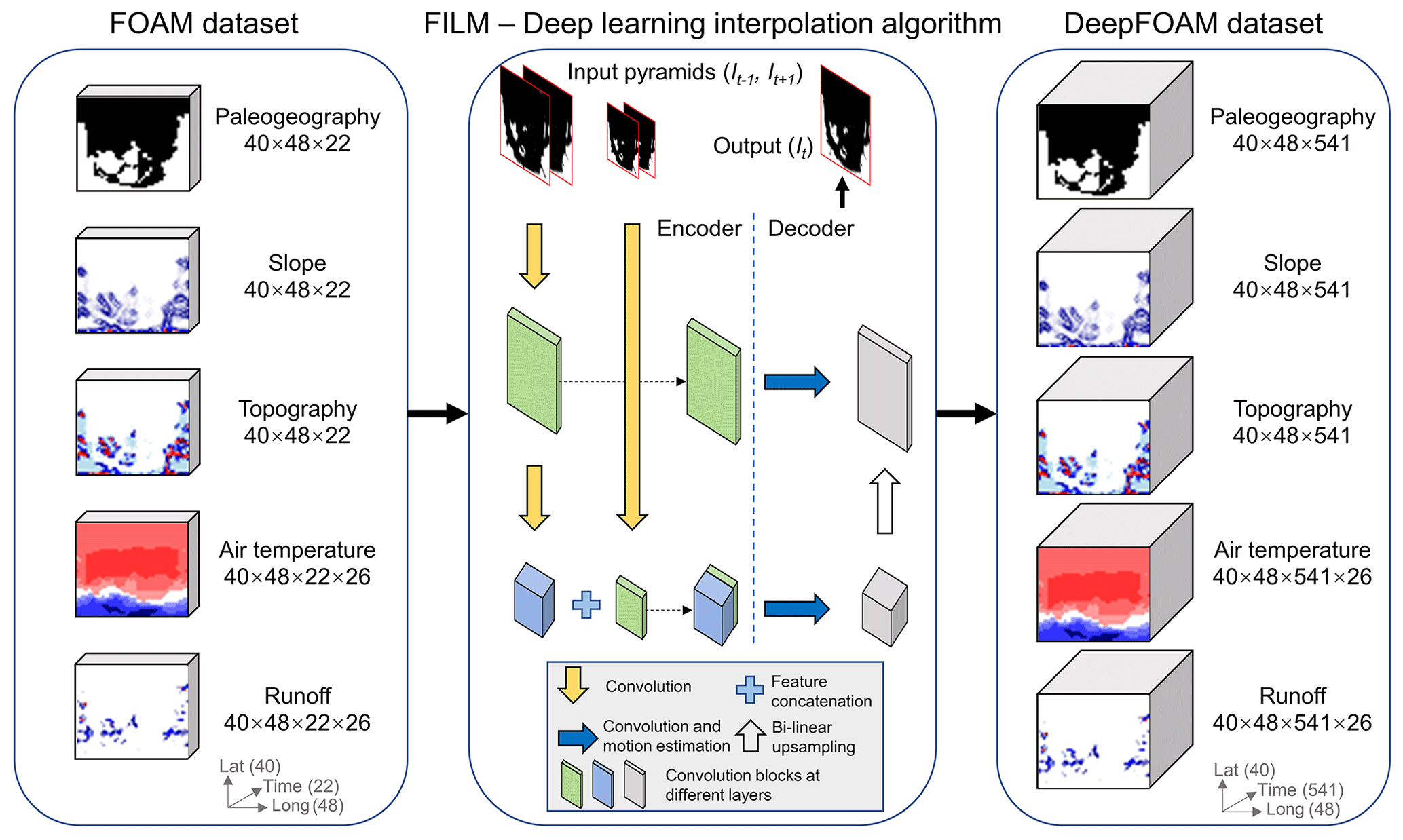
Figure 1Deep learning interpolation workflow for the FOAM dataset and simplified overview of FILM. Numerical annotations represent the dataset dimensions; e.g. for original air temperature, 40 and 48 refer to the horizontal and vertical geographic spans, 22 represents the time intervals, 26 represents the different CO2 concentration levels. I(t−1) and I(t+1) represent the two input frames; It is the intermediate frame. The convolution step is the matrix operation to obtain high-level feature representations; motion estimation is the change estimation achieved by the convolution operation; concatenation means the unification of two matrices of the same dimension to amalgamate features from different levels in the input pyramids; bi-linear up sampling is the technique used to reconstruct a frame from the high-level feature representation. The FILM overview is simplified based on Fig. 2 in Reda et al. (2022); we refer the reader to Reda et al. (2022) and Goodfellow et al. (2016) for further details of these techniques.
FILM is a U-shaped CNN encompassing both encoders and decoders (Fig. 1). Convolution, the fundamental operation in any CNN, involves multiplication between the image matrix and the filters, which are typically smaller matrices. This convolutional operation yields a summarized representation of the original images. Deep CNNs employ hundreds or thousands of such filters to discern features in images such as shape, brightness and patterns (Hinton et al., 2006; Goodfellow et al., 2016). The encoder module in FILM serves to extract high-level feature representations from input images. This is accomplished via its specialized pyramidal architecture that encompasses seven levels of feature extractors. These range from a fine level (high resolution) to a coarse level (low resolution), effectively allowing FILM to detect both fine and coarse changes in the images, with each successive extractor operating on an input frame with half the resolution of the previous level's inputs. These input frames then undergo several layers of convolution blocks to extract high-level feature representations and bi-directional motion between the input and interpolated frames. The feature representations, coupled with the bi-directional motion, synthesize the high-level representations of the intermediate frame. The decoder module of FILM then uses these high-level representations to reconstruct the intermediate images. During the training process, the weights in the convolution blocks within both the encoder and the decoder are continually adjusted to minimize the differences between the model-predicted images and the training images. Having undergone training with over 100 000 unique videos, the pre-trained FILM model exhibits the capability to discern rotation, scaling, colour changes, movements, and more intricate deformations, making it ideally suited for creating interpolation images for novel tasks.
We use the pre-trained FILM model to create interpolated images without conducting additional training. By running the FILM model with our image dataset (comprising 22 images for a given CO2 concentration at each time interval, n), it yields 21, n−1, interpolation images. During the second round of prediction, both the original and the interpolated images are used to generate further interpolation images between the original images and the first-round interpolation images. By iterating this operation k times, (2 interpolation images are generated in total, and 2k−1 images are formed between each of the two original images. Given that the maximum age gap between the original model forcing is 55 Myr, we executed six iterations of prediction to produce 63 interpolation images between each pair of original images and selected at most 54 out of the 63 images to represent the dataset for each million-year time point. These selections were made evenly across the 63 images to ensure a uniform and representative sampling for each million-year interval in the dataset.
3.1 Validation of interpolation using a paleoDEM dataset
While the FILM model has demonstrated a robust ability to interpolate complex changes between input and intermediate frames, largely due to extensive training on over 100 000 videos, its performance has not yet been scrutinized in the context of paleogeographic and paleoclimate datasets. To test this application, we first apply the FILM model to a high-time-resolution paleo-digital elevation model (paleoDEM) dataset (Scotese and Wright, 2018) that delineates the evolving distributions of land and oceans over the past 540 million years in 5-million-year intervals. By partitioning the paleoDEM dataset into input and intermediate frames, we could contrast the FILM-predicted frames with the actual intermediate frames, quantifying their disparities. The similarity between the predicted and actual frames serves as a testament to FILM's efficacy in capturing plate movements and transformations.
The paleoDEM dataset comprises 109 files, and each file includes estimations of land surface elevation and ocean depth, measured in metres, at a resolution of 1×1°. Hence, the paleoDEM dataset is a 361×181-dimensional dataset where 361 represents longitude (ranging from −180 to 180) and 181 denotes latitude (ranging from −90 to 90). To make the paleoDEM dataset comparable with our 48×40-dimensional dataset, we applied nearest-neighbour interpolation, a downsampling algorithm, to downscale the paleoDEM resolution to 48×40 by assigning the values of the closest pixel to the new pixel locations. Moreover, any location with elevation values greater than zero was characterized as land (denoted by 255 in pixel values), with the remainder classified as oceans (denoted by 0 in pixel values).
The paleoDEM dataset was partitioned into distinct input and output datasets using temporal intervals of 10, 20, and 40 Myr. This strategy facilitated three separate validation procedures. In the first validation approach, we use a 10 Myr interval. The paleoDEM sequences from 540 Ma, 530 Ma, etc., up to 0 Ma, were designated as the input dataset. Correspondingly, the sequences from 535, 525 Ma, and so forth, until 5 Ma, were selected as the output dataset for the FILM model outputs to be compared against. For the second validation process, we adopted a 20 Myr interval. This time, the input dataset comprised paleoDEM sequences from 540, 520 Ma, etc., down to 0 Ma. The sequences from 535, 530, 525 Ma, etc., to 5 Ma served as the output dataset. An identical procedure was executed for the third validation scheme but with a 40 Myr interval. In each case we use the input dataset to make interpolation frames using FILM, and by comparing the predicted frames with the real frames in the output dataset, the model's predictive accuracy can be assessed.
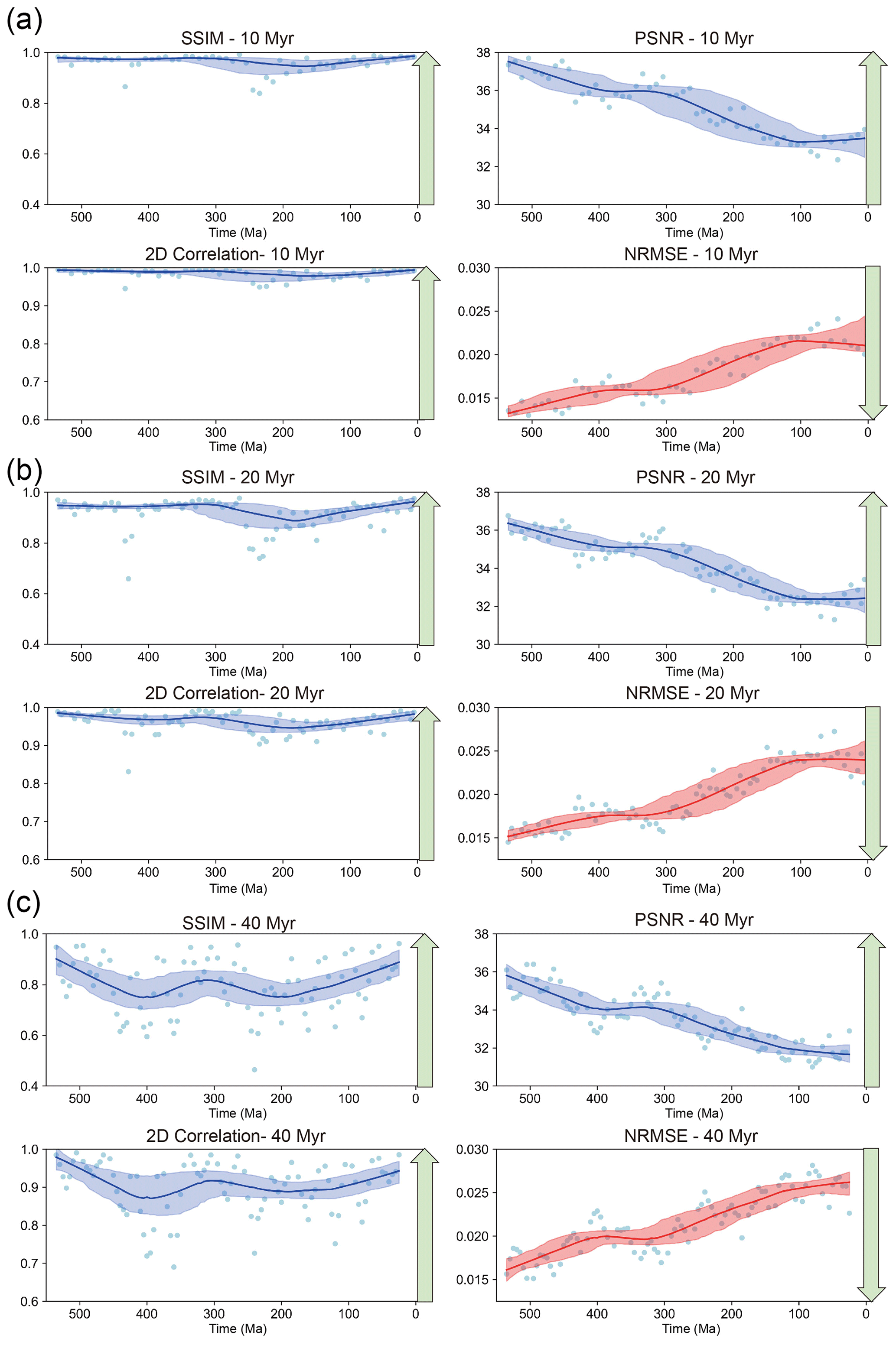
Figure 2Comparative evaluation of performance utilizing (a) 10 Myr, (b) 20 Myr, and (c) 40 yr intervals within the paleoDEM dataset. The blue line represents the LOWESS (locally weighted scatterplot smoothing) fitting curve with a fraction of 0.4, serving as an indicator of the central trend. The light-blue-shaded bands illustrate the confidence interval, derived from a 1000-resampling bootstrap method and providing a measure of the precision of and uncertainty in the estimated fit. The normalized root square of the mean square error (NRMSE) is represented in a red colour because it signifies error; thus its trend is converse to those of the three other metrics. The green arrows indicate the direction of better performance. See the main text for detailed discussions.
Table 1Numerical evaluation using the paleoDEM dataset.
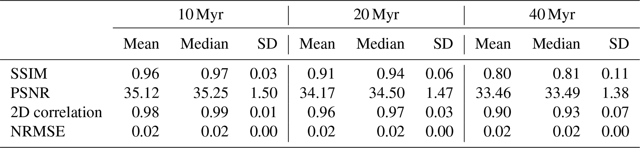
SD: standard deviation. See Sect. 3.1 for other abbreviations.
For a systematic and comprehensive investigation of the FILM model performance, we calculate the structural similarity index (SSIM), peak signal-to-noise ratio (PSNR), two-dimensional correlation, and normalized root square of the mean square error (NRMSE), which are the most widely utilized performance measurements for frame interpolation (Wang et al., 2004; Dong et al., 2023). These widely accepted metrics can help us gauge differences between the actual intermediate frames and the predicted frames. SSIM is a metric to detect perceived changes that takes into account luminance, contrast, and structural information of the image. Given the real intermediate frame IR(xy) and the FILM-predicted frame , the SSIM is defined as
where and are the mean of and IR, and are the variance of and IR, is the covariance between and IR, and c1 and c2 are constants to avoid instability when the denominator is close to zero. Values of SSIM range from −1 to 1, representing inversely identical and identical images, respectively.
The PSNR is a ratio between the maximum possible power of the image and the power of corrupting noise that affects the fidelity of the image's representation; it is defined as
where L is the maximum pixel value (255 for our images) and N is the number of pixels in the image. The greater the value of PSNR, the better the performance of the frame interpolation.
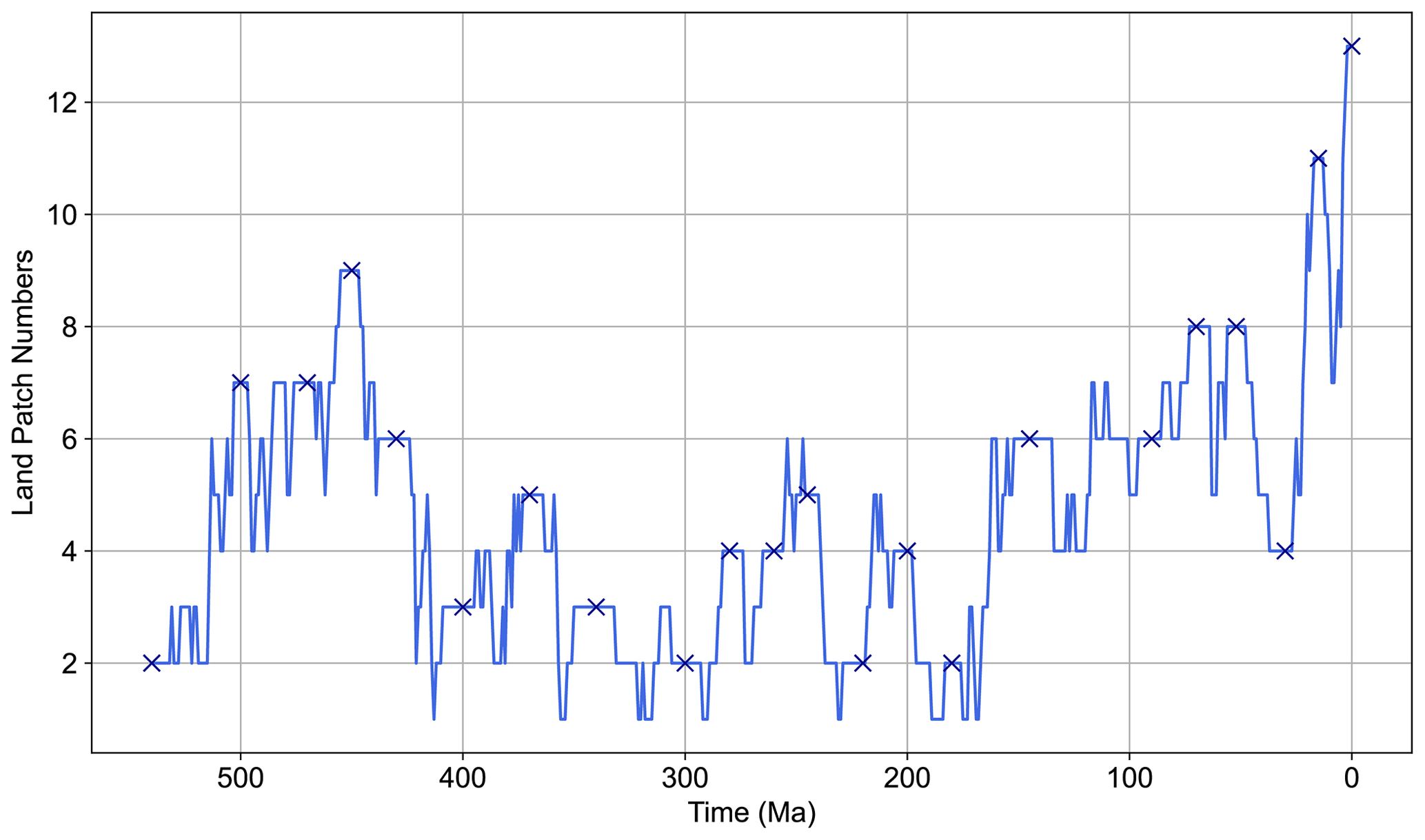
Figure 3Temporal evolution of land patch density using paleoDEM from 540 Ma to the present. This figure indicates an overall increase in land patch density in the paleoDEM dataset, attributed to the inclusions of more details in the more recent frames. This increasing trend may account for the patterns observed in PSNR and NRMSE. A land patch is defined as a contiguous grouping of land pixels. The density is calculated by dividing the number of land patches by the total frame size (40×48). The dark-blue crosses indicate the 22 time intervals used in the FOAM dataset.
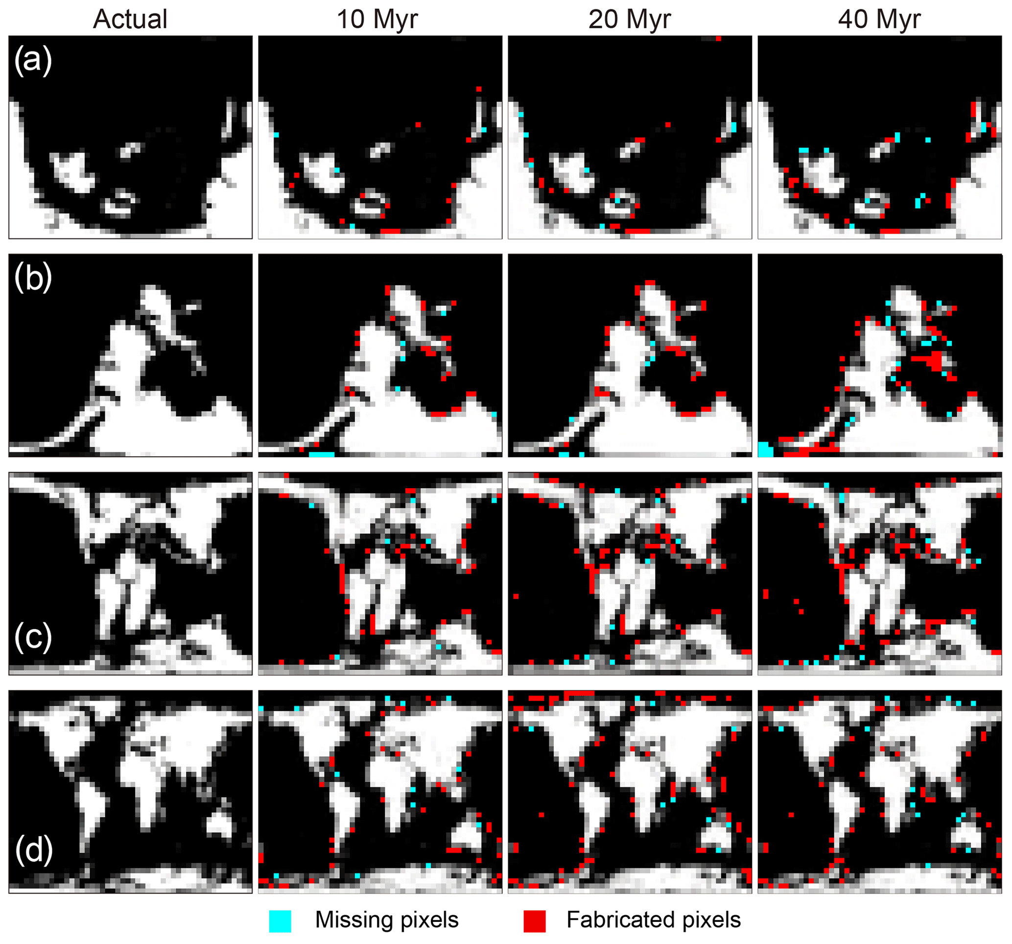
Figure 4Comparative visualization of actual paleoDEM and model-predicted frames at selected time intervals. This figure illustrates the comparative visualizations at (a) 535 Ma, (b) 315 Ma, (c) 105 Ma, and (d) 25 Ma. The grey pixels represent areas impacted by nearest-neighbour downsampling in the paleogeographic maps. The missing pixels indicate areas present in the original frames but absent in the model-predicted frames; the fabricated pixels show areas absent in the original frames but present in the model-predicted frames.
The two-dimensional correlation is defined as the Pearson correlation coefficient calculated over the two dimensions of IR(xy) and . Values of two-dimensional correlation are between −1 and 1, where 1 indicates the two images are identical, 0 means the images are uncorrelated, and −1 means the images are inversely identical. The NRMSE measures the differences in pixel values between IR(xy) and . In contrast to the other metrics, lower NRMSE values indicate better performance (range between 0 and 1).
Figure 2 and Table 1 detail the quantitative assessments derived from our implemented numerical metrics, indicating the performance of the FILM technique when applied to the paleoDEM dataset. During the validation phase, using a 10 Myr interval, the frames predicted by FILM demonstrated remarkable congruity with the actual frames. This is evidenced by the high values of SSIM, PSNR, and two-dimensional correlation and a low value of NRMSE. The SSIM and 2D correlation maintain consistently high values throughout the entire time span from 540 to 0 Ma. This highlights the consistent performance of FILM and its capacity to capture the paleogeographic reorganization in the paleoDEM dataset across Phanerozoic timescales.
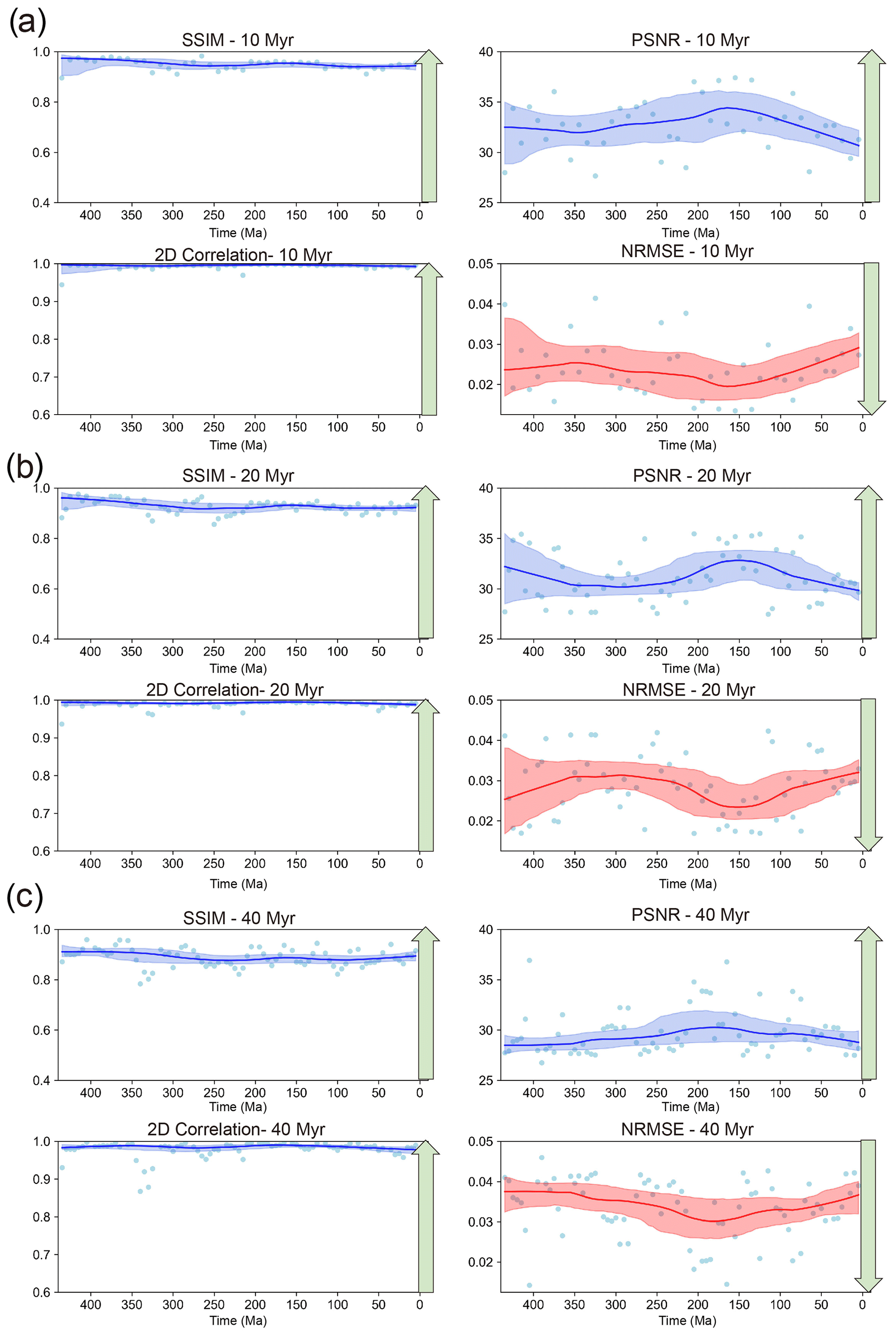
Figure 5Comparative evaluation of performance utilizing (a) 10 Myr, (b) 20 Myr, and (c) 40 Myr intervals within the surface air temperature (SAT) dataset. See Fig. 2 for detailed explanations of the image symbols.
Despite good performance in general, the PSNR and NRMSE depict a trend over time, with PSNR values decreasing and NRMSE values increasing over time – both suggesting a poorer fit to the real intermediate frames at time points closer to the present day. The observed trend is somewhat expected as the maps that become closer to the present day – and can draw on larger geological evidence bases – tend to exhibit more fine-scale features, such as land patches depicted as only 1 pixel or a few pixels in the frames (Fig. 3). During frame interpolation, fine-scale features such as minor land patches are more easily overlooked. Consequently, metrics like PSNR and NRMSE, which quantify the pixel discrepancies between the predicted and actual frames, underscore this pattern of detail loss.
For the comparison at 10 and 20 Myr intervals, a high degree of similarity between the predicted and actual frames was discernible, as evidenced by the mean values of SSIM exceeding 0.8, 2D correlation over 0.9, PSNR above 32, and NRMSE less than 0.025. For the 40 Myr interval validation, the mean values of SSIM were greater than 0.7, the mean values of 2D correlation were above 0.80, the mean values of PSNR were over 31, and the mean values of NRMSE remained below 0.03. As anticipated, the performance deteriorates when the time interval is increased (Argaw and Kweon, 2022), which can be attributed to the more significant changes between the two input frames. Interestingly, the SSIM and 2D correlation show a particular decrease in performance at around 220 and 420 Ma. This may be due to more complex plate movements around these times which the algorithm finds more difficult to predict.
In addition to the numerical evaluation, we also performed visual inspections to detect obvious discrepancies between the original frames and the predicted frames. Across different time periods, predicted frames were generally visually comparable to original ones (see Fig. 2 for numerical estimations). The major deviations between the predicted and original frames were attributable to missing pixels or mismatched pixel values, and there were no changes in the placements of major landmasses (Fig. 4). Given that the mean temporal interval for SCION model forcings is approximately 25 Myr, our numerical assessments and visual evaluations in comparing the FILM-predicted frames with the actual frames from the paleoDEM dataset suggest that FILM possesses the capability to discern plate movements and transformations on a timescale appropriate to building interpolation frames for the SCION model forcings. Nevertheless, the FILM method creates a significant number of unmatched pixels compared to the original frames, which would alter climatic outputs of GCMs and linked biogeochemical calculations, especially as small introduced islands would be expected to have high runoff and chemical weathering rates (Park et al., 2020).
Table 2Numerical evaluation using the Phanerozoic SAT dataset.
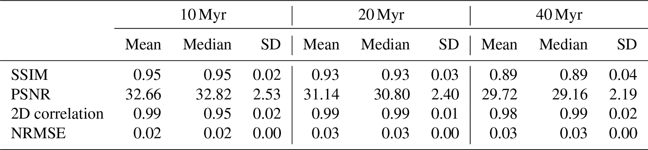
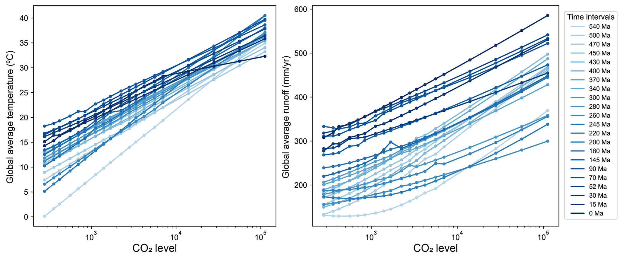
Figure 6Global average surface air temperature and average continental runoff over CO2 levels in the FOAM dataset. The representation is colour-coded with a descending blue gradient, where light blue represents more ancient conditions and dark blue denotes more recent scenarios. Note that the 0 Ma curve is built from only one CO2 level (preindustrial), with an arbitrary increase in temperature and runoff applied when CO2 levels change.
3.2 Validation of interpolation using a GCM dataset
We now apply the FILM model to a high-time-resolution dataset of Phanerozoic surface air temperature (SAT; Scotese et al., 2021). This dataset is based on GCM simulations (HadCM3L; Valdes et al., 2021), with the CO2 level in the simulation inferred from global temperature proxies such as biogenic calcite and apatite δ18O and lithological climate indicators. The Phanerozoic SAT dataset shares the same spatial resolution as the paleoDEM dataset, with a resolution of 1×1°, and comprises a 361×181 data array. The SAT dataset features a 10 Myr temporal resolution from 540–450 Ma and a 5 Myr resolution from 450 Ma to the present. We selected the SAT dataset from 450 Ma onward to ensure consistent validation.
During validation, we used the SAT dataset without downscaling and conducted the same numerical validation considering temporal intervals of 10, 20, and 40 Myr. Similarly to the results for the paleoDEM dataset, interpolations using a 10 Myr interval demonstrated close congruence with the actual frames, as evidenced by high values of SSIM, 2D correlation, and PSNR, along with low values of NRMSE from 450 Ma to the present (see Fig. 5; Table 2). Moreover, compared to the paleoDEM dataset, the interpolation performance of SAT across different time intervals exhibited more consistent results, as indicated by closer evaluation metrics (Table 2). This is likely because the temperature fields did not contain such sharp transitions between land and ocean.
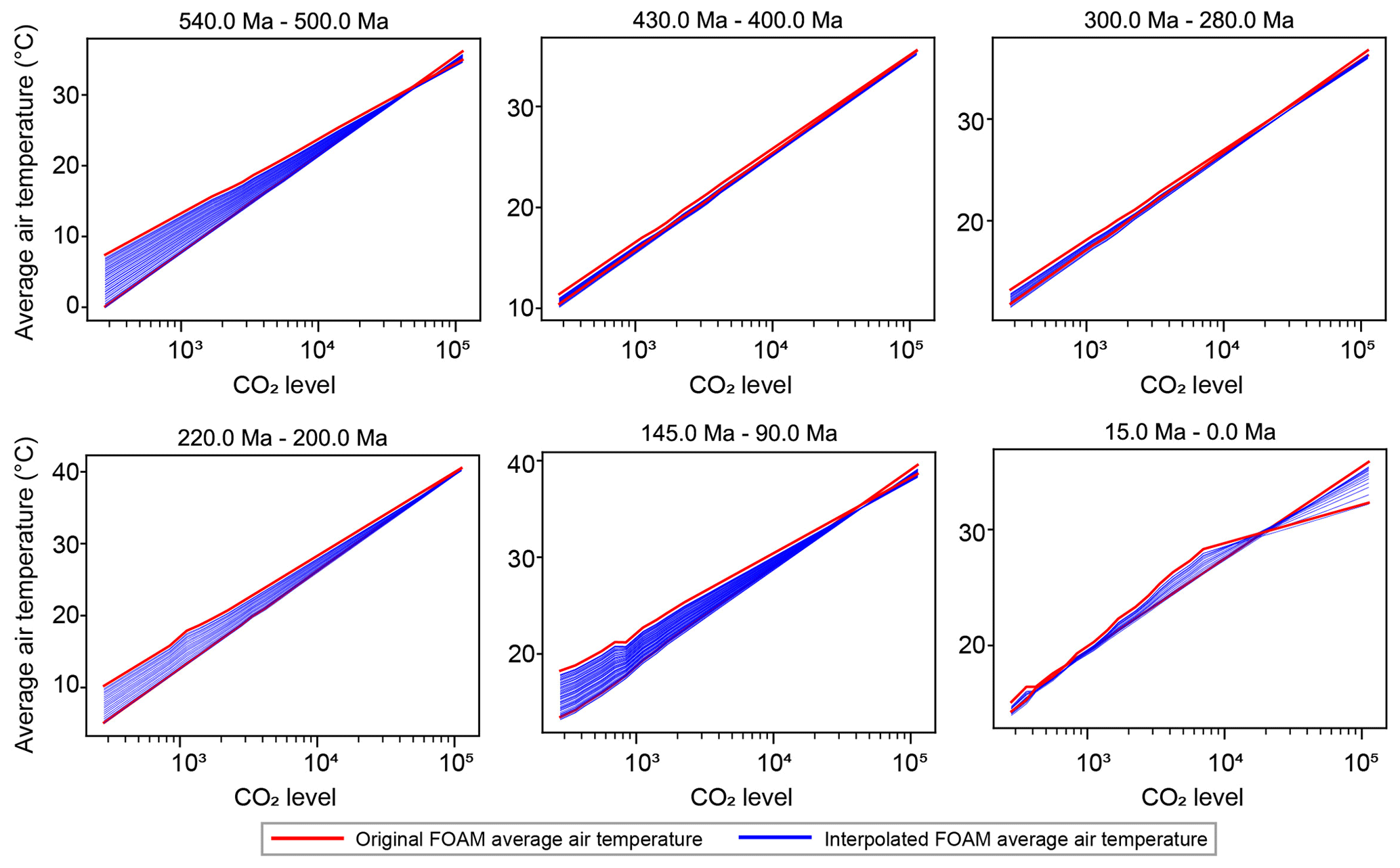
Figure 7Trends in global temperature changes corresponding to varying CO2 levels. Each subplot features 1 of the 21 distinct time intervals between members of the FOAM dataset. Within each subplot, the red lines delineate the key frame average temperature variations and the blue lines show the deep-learning-interpolated average temperature for each 1 Myr interval. See Fig. A1 for all 21 subplots.
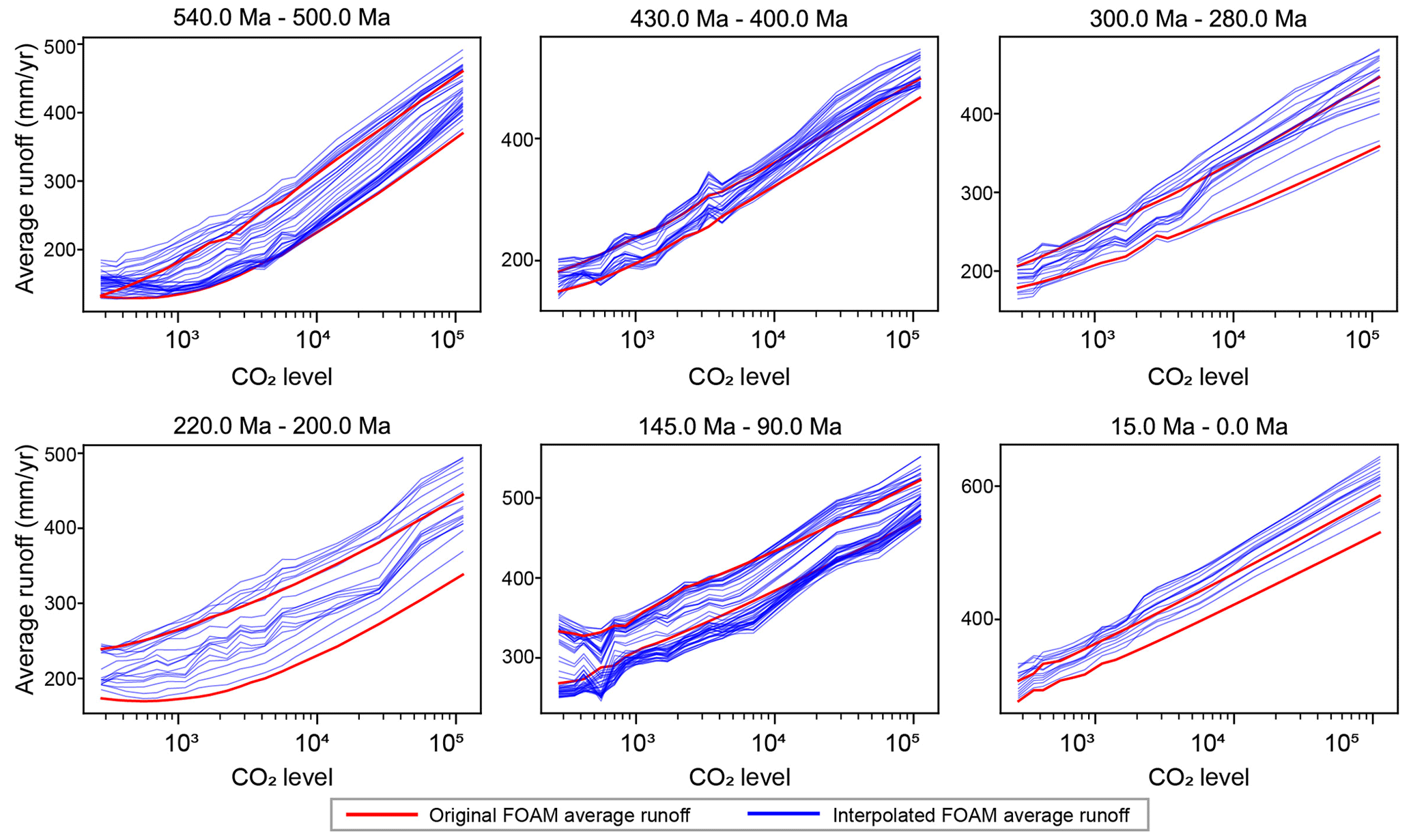
Figure 8Trends in runoff changes corresponding to varying CO2 levels. As with Fig. 7, the subplots represent the runoff changes between the original runoff outputs from the FOAM dataset. The red lines are the original average runoff in the FOAM dataset, and blue lines are deep-learning-interpolated data. See Fig. A2 for all 21 subplots.
3.3 Output and validation of intermediate FOAM temperature and runoff datasets
We now focus on the temperature and runoff data in our interpolated DeepFOAM dataset. Given the established correlation between increased CO2 levels and a rise in global average temperature and total runoff, we anticipated that our interpolated data should mirror this trend if FILM is effectively applied to our dataset. Consequently, we test the alignment of interpolated temperature and runoff trends with those of the original model forcings. The SCION model forcing dataset is constructed with 26 distinct CO2 levels, encompassing an extensive range of CO2 concentrations, from 10 to 112 000 ppm (Mills et al., 2021). This dataset has been extrapolated and in-filled from an average of five runs of FOAM per continental configuration, which was made possible because of a predictable logarithmic response of temperature and runoff to CO2 change in the model. Such a wide range of CO2 levels is required to aid in model spinup where the model conditions can be far from equilibrium. Typically, Phanerozoic runs of the SCION model do not stray beyond the range of the initial dataset from FOAM. Figure 6 plots the global average temperature and runoff over these 26 CO2 levels, with each of the 22 lines representing a unique time interval (i.e. continental configuration) in FOAM. It exhibits an overall upward trend in temperature and runoff as CO2 concentrations ascend, and the relationship between CO2 and climate is dependent on the continental configuration (e.g. Wong Hearing et al., 2021) and solar constant. It should be briefly noted that the 0 Ma climate ensemble is computed from only one run of FOAM at preindustrial CO2 levels, adding a generalized trend for higher and lower CO2 levels. This is because the SCION model is not designed to perform variable-CO2 simulations in present-day conditions and only uses this state for spinup and parameter tuning.
Given the known behaviour of the climate model FOAM, our FILM-interpolated temperature and runoff grids should exhibit similar patterns and serve as a method to evaluate the effectiveness of the FILM interpolation technique for this purpose. Figure 7 plots global average temperature changes in response to varying CO2 levels for each of the intermediate frames produced by FILM. The FOAM dataset contains values across 22 time intervals, leading to the 21 subplots (all subplots in the Appendix) that show the average temperature changes for all intermediate frames between these 22 time intervals. The interpolated temperature values are well-aligned with the original dataset, displaying a consistent trend for escalating CO2 concentrations. Figure 8 shows the runoff trends in response to varying CO2 levels. Similar to the temperature trends, they exhibit patterns with respect to CO2 that are analogous to those of the original runoff data. Given the more scattered distributions and more substantial changes in runoff between continental configurations, the interpolated average runoff exhibits a more varied pattern between the key frame images, with interpolated intermediate runoff averages that can be both higher and lower than the end-members from which they are derived. Capturing runoff changes on small land patches remains a particularly challenging task for the deep learning methods, unlike the case with homogeneous variables like temperature, where FILM is more adept.
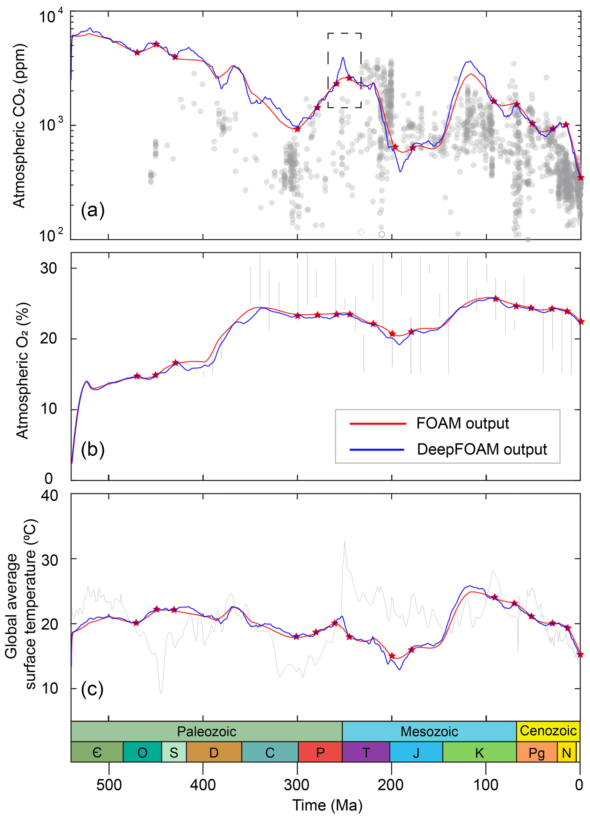
Figure 9Phanerozoic output comparisons between SCION–FOAM and SCION–DeepFOAM. (a) Atmospheric CO2 concentration (proxy data represented by circles; sources: Foster et al., 2017; Witkowski et al., 2018), (b) atmospheric O2 concentration (proxy data represented by vertical lines; sources: Glasspool and Scott, 2010; Lenton et al., 2016), and (c) global average surface temperature (proxy data represented in grey; source: Scotese et al., 2021). The red stars represent the time intervals of 20 Myr or less in the FOAM dataset. The dashed box in panel (a) marks the significant CO2 increase at 253 Ma.
We now run the SCION model (version 1.1.6; http://github.com/bjwmills/SCION, last access: 10 April 2023) subject to the new DeepFOAM dataset, which directly replaces the FOAM dataset used in the standard model. This update requires no additional modification of the SCION model. The key model predictions for atmospheric CO2, atmospheric O2, and global average surface temperature are shown in Fig. 9. These new model predictions follow the original model closely at the defined time points for the FOAM dataset, but they have a more detailed structure between these points and show several interesting deviations from the previous model, which are due to the new FILM-interpolated climate fields which, in turn, have replaced linear interpolation between the widely spaced previous fields.
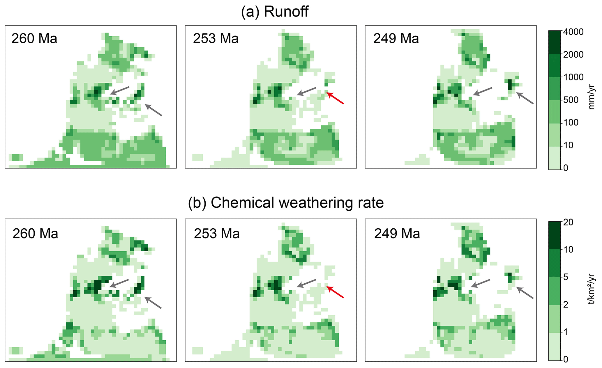
Figure 10Runoff (a) and chemical weathering rates (b) for 260, 253, and 249 Ma. During the 260–245 Ma period, the low-latitude regions surrounding the Paleo-Tethys Ocean exhibit high runoff and corresponding high weathering (highlighted by grey arrows). These characteristics are derived from the FOAM dataset. However, during the 253 Ma interval, the deep learning method predicts reduced runoff and corresponding decreased weathering. This reduction is primarily attributed to the lowered runoff in eastern low-latitude plates, such as northern and/or southern China (marked by the red arrow).
Most notably, the SCION–DeepFOAM output for atmospheric CO2 shows a warming spike around the Permian–Triassic boundary and a cooling spike in the Early Jurassic. These results are in line with geological evidence for extreme warmth during the Permian–Triassic extinction (Berner, 2002; Fielding et al., 2019; Yang et al., 2021; Wu et al., 2024) and a cool Early Jurassic (Scotese et al., 2021). To investigate these outputs, Fig. 10 plots variations in runoff and chemical weathering rates spanning 260–245 Ma. The original FOAM dataset contains runoff values at 260 and 245 Ma, both of which indicate high runoff in the low latitudes (marked by grey arrows in Fig. 10) surrounding the Paleo-Tethys Ocean. As a consequence, chemical weathering rates in these zones are comparably high, being influenced by both runoff and temperature (Maffre et al., 2018; Mills et al., 2021). Contrastingly, for the 253 Ma interval, predicted via deep learning, the South China Plate exhibits diminished runoff values and correspondingly lower chemical weathering rates (marked by red arrows in Fig. 10). The observed decrease in weathering aligns with geological records which highlight significant aridity in China at the time of the Permian–Triassic boundary (Cui and Cao, 2021; Xu et al., 2023), and it is this reduced chemical weathering that leads to elevated atmospheric CO2 predictions for this time in the SCION model. However, this result requires further scrutiny, as while the deep learning approach affords a continuous dataset, there are no specific physical mechanisms underpinning the results. In reality, aridity here may have been due to extreme warming following the emplacement of the Siberian Traps, which is not included in our model. Moreover, variations in different paleogeographic map versions (e.g. southern China is smaller in Marcilly et al., 2021, than in Scotese and Wright, 2018) or image processing techniques such as downscaling or upscaling, as well as the large time intervals (>10 Myr) between the original frames, may further complicate the results. Testing this hypothesis still requires a climate model run for the period of interest. Notably, the deep learning interpolation can produce intervals of climatic changes in climate-biogeochemical models, but it does not allow for the resolution of climate events that were previously undetectable. For example, the Hirnantian ice age cannot be represented in the SCION model using the DeepFOAM dataset because various suggested mechanisms for Hirnantian cooling, such as rapid weathering and a decrease in degassing due to arc–continent collision (Macdonald et al., 2019) and weathering amplification due to land plant evolution (Lenton et al., 2012), are not incorporated in the current SCION model used in this study (Mills et al., 2021).
We show that deep learning can produce realistic continuous plate geographical motions, as well as associated paleoclimates, from snapshots up to 40 Myr apart. The FILM deep learning technique can be applied to the forcing set for the SCION climate-biogeochemical model, which reduces the need for the model to interpolate linearly between time points and thus allows a greater degree of climate variability, as well as making the model easier to use for testing specific events at known times that are not within its original forcing set. This alteration produces new intervals of climatic change in the climate-biogeochemical model, but it does not allow it to resolve any climate events that it previously could not, such as the Hirnantian ice age. It should also be noted that variations in different paleogeographic map versions, variations in image processing techniques, and the large time intervals (>10 Myr) and relatively coarse resolution of original frames can affect the accuracy of the interpolation. Particularly, the efficacy of interpolating runoff data, compared to those of paleogeography and temperature, is diminished by their heterogeneous distribution. The new forcing set creates important differences in the model output, demonstrating the utility of deep learning for rapid preliminary analysis, but further conclusions on these differences rely on performing new climate model runs at these specific times. It is intuitively understood that these interpolation results can be enhanced with a higher-resolution original dataset, a presumption corroborated by the paleoDEM validation and the SAT validation. In the paleoDEM and the SAT validation processes, interpolation results derived from a 10 Myr interval exhibited superior accuracy compared to those from 20 and 40 Myr intervals. Thus, future work to link paleoclimate and biogeochemistry should aim to run climate models at least every 10 Myr. Combing the deep learning interpolation to upscale this to 1 Myr or finer time resolutions would allow more precise investigation of the paleoclimate and fossil record for specific events, and may also permit new approaches where modelled surface processes (e.g. vegetation) are able to be distributed in space from one time step to the next.
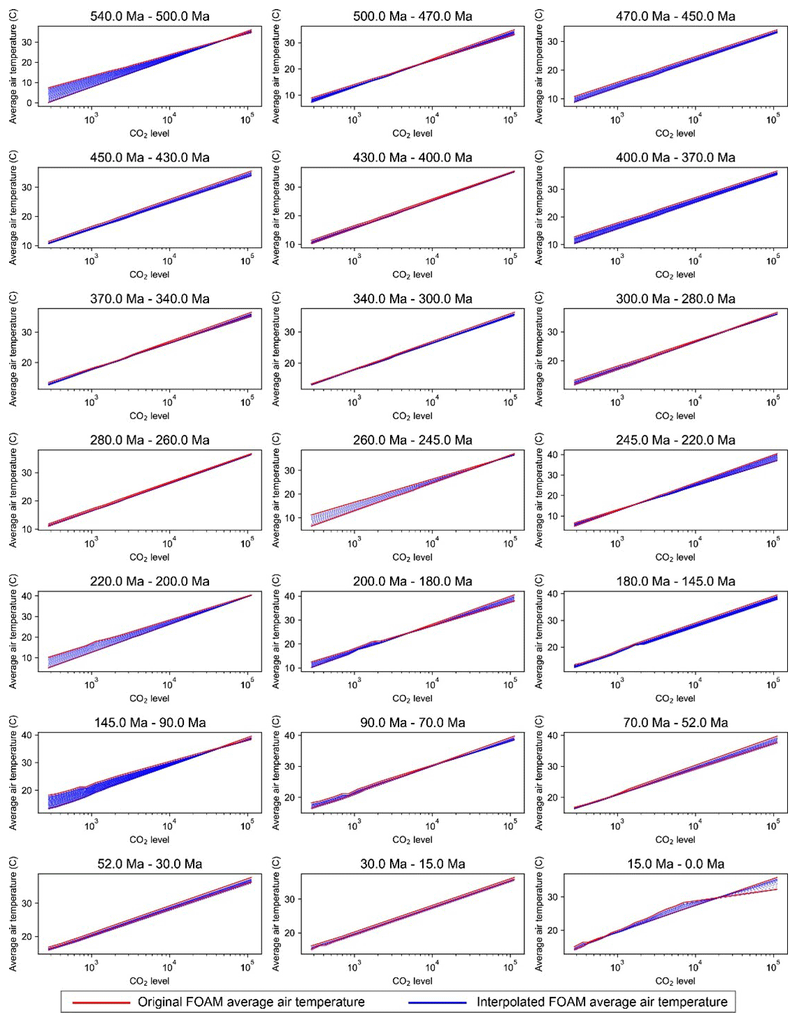
Figure A1All the subplots of the trends in global temperature changes corresponding to varying CO2 levels. Each subplot features 1 of the 21 distinct time intervals between members of the FOAM dataset. Within each subplot, the red lines delineate the key frame average temperature variations and the blue lines show the deep-learning-interpolated average temperature for each 1 Myr interval.
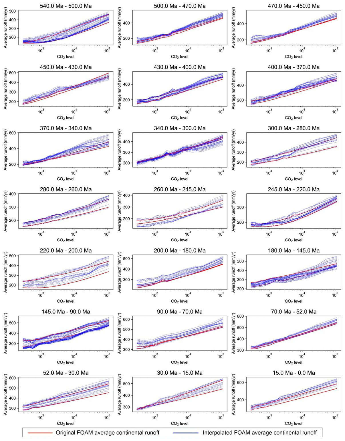
Figure A2All the subplots of the trends in global runoff changes corresponding to varying CO2 levels. Each subplot features 1 of the 21 distinct time intervals between members of the FOAM dataset. Within each subplot, the red lines delineate the key frame average runoff variations and the blue lines show the deep-learning-interpolated average runoff for each 1 Myr interval.
The FILM code is available at https://github.com/google-research/frame-interpolation (last access: 10 April 2023) and a Zenodo repository (Reda et al., 2024, https://doi.org/10.5281/zenodo.10602810) under the Apache License 2.0. SCION v1.1.6 code is available at https://github.com/bjwmills/SCION (last access: 10 April 2023) and is permanently archived on Zenodo (Mills, 2023, https://doi.org/10.5281/zenodo.7790169); codes for figure creation are archived on Zenodo (Zheng, 2024, https://doi.org/10.5281/zenodo.10578608).
DZ, ASM, and BJWM designed this study; YG and YD provided the FOAM dataset; DZ performed the interpolation and validation; DZ and BJWM wrote the manuscript draft; all authors reviewed and edited the manuscript. The project administration was carried out by BJWM.
The contact author has declared that none of the authors has any competing interests.
Publisher's note: Copernicus Publications remains neutral with regard to jurisdictional claims made in the text, published maps, institutional affiliations, or any other geographical representation in this paper. While Copernicus Publications makes every effort to include appropriate place names, the final responsibility lies with the authors.
The authors would like to thank Stephen Hunter for useful discussions. Dongyu Zheng is funded by the National Natural Science Foundation of China (grant no. 42202125), Natural Science Foundation of Sichuan Province (grant no. 2024NSFSC0828), and IUGS Deep-time Digital Earth Big Science Program. Benjamin J. W. Mills is funded by UKRI project NE/X011208/1.
This research has been supported by the National Natural Science Foundation of China (grant no. 42202125), Natural Science Foundation of Sichuan Province (grant no. 2024NSFSC0828), and UKRI project NE/X011208/1.
This paper was edited by Marko Scholze and reviewed by two anonymous referees.
Argaw, D. M. and Kweon, I. S.: Long-term video frame interpolation via feature propagation, in: Proceedings of the IEEE/CVF Conference on Computer Vision and Pattern Recognition, 3543–3552, 2022.
Berner, R. A.: Examination of hypotheses for the Permo-Triassic boundary extinction by carbon cycle modeling, P. Natl. Acad. Sci. USA, 99, 4172–4177, https://doi.org/10.1073/pnas.032095199, 2002.
Chen, G., Cheng, Q., Lyons, T. W., Shen, J., Agterberg, F., Huang, N., and Zhao, M.: Reconstructing Earth's atmospheric oxygenation history using machine learning, Nat. Commun., 13, 5862, https://doi.org/10.1038/s41467-022-33388-5, 2022.
Cui, C., and Cao, C.: Increased aridity across the Permian–Triassic transition in the mid‐latitude NE Pangea, Geol. J., 56, 6162–6175, 2021.
Dong, J., Ota, K., and Dong, M.: Video frame interpolation: A comprehensive survey, ACM T. Multim. Comput., 19, 1–31, https://doi.org/10.1145/3556544, 2023.
Donnadieu, Y., Pierrehumbert, R., Jacob, R., and Fluteau, F.: Modelling the primary control of paleogeography on Cretaceous climate, Earth Planet. Sc. Lett., 248, 426–437, 2006.
Fielding, C. R., Frank, T. D., McLoughlin, S., Vajda, V., Mays, C., Tevyaw, A. P., Winguth, A., Winguth, C., Nicoll, R. S., Bocking, M., and Crowley, J. L.: Age and pattern of the southern high-latitude continental end-Permian extinction constrained by multiproxy analysis, Nat. Commun., 10, 385, https://doi.org/10.1038/s41467-018-07934-z, 2019.
Foster, G. L., Royer, D. L., and Lunt, D. J.: Future climate forcing potentially without precedent in the last 420 million years, Nat. Commun., 8, 14845, https://doi.org/10.1038/ncomms14845, 2017.
Glasspool, I. J. and Scott, A. C.: Phanerozoic concentrations of atmospheric oxygen reconstructed from sedimentary charcoal, Nat. Geosci., 3, 627–630, 2010.
Goddéris, Y., Donnadieu, Y., Le Hir, G., Lefebvre, V., and Nardin, E.: The role of palaeogeography in the Phanerozoic history of atmospheric CO2 and climate, Earth-Sci. Rev., 128, 122–138, https://doi.org/10.1016/j.earscirev.2013.11.004, 2014.
Goddéris, Y., Donnadieu, Y., and Mills, B. J. W.: What models tell us about the evolution of carbon sources and sinks over the Phanerozoic, Annu. Rev. Earth Planet. Sci., 51, 471–492, 2023.
Hinton, G. E., Osindero, S., and Teh, Y.-W.: A Fast Learning Algorithm for Deep Belief Nets, Neural Comput., 18, 1527–1554, 2006.
Goodfellow, I., Bengio, Y., and Courville, A.: Deep learning, MIT Press, ISBN 9780262035613, 2016.
Lenton, T. M. and Watson, A. J.: Biotic enhancement of weathering, atmospheric oxygen and carbon dioxide in the Neoproterozoic, Geophys. Res. Lett., 31, L05202, https://doi.org/10.1029/2003GL018802, 2004.
Lenton, T. M., Crouch, M., Johnson, M., Pires, N., and Dolan, L.: First plants cooled the Ordovician, Nat. Geosci., 5, 86–89, 2012.
Lenton, T. M., Dahl, T. W., Daines, S. J., Mills, B. J. W., Ozaki, K., Saltzman, M. R., and Porada, P.: Earliest land plants created modern levels of atmospheric oxygen, P. Natl. Acad. Sci. USA, 113, 9704–9709, 2016.
Longman, J., Mills, B. J. W., Donnadieu, Y., and Goddéris, Y.: Assessing Volcanic Controls on Miocene Climate Change, Geophys. Res. Lett., 49, 1–11, https://doi.org/10.1029/2021GL096519, 2022.
Macdonald, F. A., Swanson-Hysell, N. L., Park, Y., Lisiecki, L., and Jagoutz, O.: Arc-continent collisions in the tropics set Earth’s climate state, Science, 364, 181–184, 2019.
Maffre, P., Ladant, J. B., Moquet, J. S., Carretier, S., Labat, D., and Goddéris, Y.: Mountain ranges, climate and weathering. Do orogens strengthen or weaken the silicate weathering carbon sink?, Earth Planet. Sc. Lett., 493, 174–185, https://doi.org/10.1016/j.epsl.2018.04.034, 2018.
Maher, K. and Chamberlain, C. P.: Hydrologic regulation of chemical weathering and the geologic carbon cycle, Science, 343, 1502–1504, 2014.
Marcilly, C. M., Torsvik, T. H., Domeier, M., and Royer, D. L.: New paleogeographic and degassing parameters for long-term carbon cycle models, Gondwana Res., 97, 176–203, 2021.
Mills, B. J. W.: bjwmills/SCION: v1.1.6 (v1.1.6), Zenodo [code], https://doi.org/10.5281/zenodo.7790169, 2023.
Mills, B. J. W., Donnadieu, Y., and Goddéris, Y.: Spatial continuous integration of Phanerozoic global biogeochemistry and climate, Gondwana Res., 100, 73–86, https://doi.org/10.1016/j.gr.2021.02.011, 2021.
Niklaus, S., Mai, L., and Liu, F.: Video frame interpolation via adaptive separable convolution, in: Proceedings of the IEEE international conference on computer vision, 261–270, 2017.
Park, Y., Maffre, P., Goddéris, Y., MacDonald, F. A., Anttila, E. S. C., and Swanson-Hysell, N. L.: Emergence of the Southeast Asian islands as a driver for Neogene cooling, P. Natl. Acad. Sci. USA, 117, 25319–25326, https://doi.org/10.1073/pnas.2011033117, 2020.
Reda, F., Kontkanen, J., Tabellion, E., Sun, D., Pantofaru, C., and Curless, B.: FILM: Frame Interpolation for Large Motion, Lect. Notes Comput. Sci. (including Subser. Lect. Notes Artif. Intell. Lect. Notes Bioinformatics), 13667 LNCS, 250–266, https://doi.org/10.1007/978-3-031-20071-7_15, 2022.
Reda, F., Kontkanen, J., Tabellion, E., Sun, D., Pantofaru, C., and Curless, B.: FILM: Frame Interpolation for Large Motion, European Conference on Computer Vision (ECCV) (ECCV), Zenodo [code], https://doi.org/10.5281/zenodo.10602810, 2024.
Reichstein, M., Camps-Valls, G., Stevens, B., Jung, M., Denzler, J., Carvalhais, N., and Prabhat: Deep learning and process understanding for data-driven Earth system science, Nature, 566, 195–204, https://doi.org/10.1038/s41586-019-0912-1, 2019.
Royer, D. L., Berner, R. A., Montañez, I. P., Tabor, N. J., and Beerling, D. J.: CO2 as a primary driver of phanerozoic climate, GSA today, 14, 4–10, 2004.
Scotese, C. R.: An atlas of Phanerozoic paleogeographic maps: the seas come in and the seas go out, Annu. Rev. Earth Planet. Sci., 49, 679–728, 2021.
Scotese, C. R. and Wright, N.: PALEOMAP Paleodigital Elevation Models (PaleoDEMS) for the Phanerozoic PaleoDEMs, PALEOMAP Project, https://www.earthbyte.org/paleodem-resource-scotese-and-wright-2018 (last access: 10 April 2023), 2018.
Scotese, C. R., Song, H., Mills, B. J. W., and van der Meer, D. G.: Phanerozoic paleotemperatures: The earth's changing climate during the last 540 million years, Earth-Sci. Rev., 215, 103503, https://doi.org/10.1016/j.earscirev.2021.103503, 2021.
Shi, Z., Xu, X., Liu, X., Chen, J., and Yang, M.-H.: Video frame interpolation transformer, in: Proceedings of the IEEE/CVF Conference on Computer Vision and Pattern Recognition, 17482–17491, 2022.
Valdes, P. J., Scotese, C. R., and Lunt, D. J.: Deep ocean temperatures through time, Clim. Past, 17, 1483–1506, https://doi.org/10.5194/cp-17-1483-2021, 2021.
Walker, J. C. G., Hays, P. B., and Kasting, J. F.: A negative feedback mechanism for the long-term stabilization of Earth's surface temperature, J. Geophys. Res.-Ocean., 86, 9776–9782, 1981.
Wang, Z., Bovik, A. C., Sheikh, H. R., and Simoncelli, E. P.: Image quality assessment: from error visibility to structural similarity, IEEE T. Image Process., 13, 600–612, 2004.
West, A. J.: Thickness of the chemical weathering zone and implications for erosional and climatic drivers of weathering and for carbon-cycle feedbacks, Geology, 40, 811–814, 2012.
Witkowski, C. R., Weijers, J. W. H., Blais, B., Schouten, S., and Sinninghe Damsté, J. S.: Molecular fossils from phytoplankton reveal secular PCO2 trend over the Phanerozoic, Sci. Adv., 4, eaat4556, https://doi.org/10.1126/sciadv.aat4556, 2018.
Wong Hearing, T. W., Pohl, A., Williams, M., Donnadieu, Y., Harvey, T. H. P., Scotese, C. R., Sepulchre, P., Franc, A., and Vandenbroucke, T. R. A.: Quantitative comparison of geological data and model simulations constrains early Cambrian geography and climate, Nat. Commun., 12, 1–11, https://doi.org/10.1038/s41467-021-24141-5, 2021.
Wu, H., Zhang, X., Xie, W., Zhang, Y., and Wang, Y.: Boost Video Frame Interpolation via Motion Adaptation, arXiv [preprint], arXiv2306.13933, 2023.
Wu, Q., Zhang, H., Ramezani, J., Zhang, F. F., Erwin, D. H., Feng, Z., Shao, L. Y., Cai, Y. F., Zhang, S. H., Xu, Y. G., and Shen, S. Z.: The terrestrial end-Permian mass extinction in the paleotropics postdates the marine extinction, Sci. Adv., 10, eadi7284, https://doi.org/10.1126/sciadv.adi7284, 2024.
Xu, G., Shen, J., Algeo, T. J., Yu, J., Feng, Q., Frank, T. D., Fielding, C. R., Yan, J., Deconink, J. F., and Lei, Y.: Limited change in silicate chemical weathering intensity during the Permian–Triassic transition indicates ineffective climate regulation by weathering feedbacks, Earth Planet. Sc. Lett., 616, 118235, https://doi.org/10.1016/j.epsl.2023.118235, 2023.
Yang, W., Wan, M., Crowley, J. L., Wang, J., Luo, X., Tabor, N., Angielczyk, K. D., Gastaldo, R., Geissman, J., and Liu, F.: Paleoenvironmental and paleoclimatic evolution and cyclo-and chrono-stratigraphy of upper Permian–Lower Triassic fluvial-lacustrine deposits in Bogda Mountains, NW China – Implications for diachronous plant evolution across the Permian–Triassic boundary, Earth-Sci. Rev., 222, 103741, https://doi.org/10.1016/j.earscirev.2021.103741, 2021.
Zheng, D.: DeepFOAM – creating Figures, Zenodo [code], https://doi.org/10.5281/zenodo.10578608, 2024.
Zheng, D., Wu, S., Ma, C., Xiang, L., Hou, L., Chen, A., and Hou, M.: Zircon classification from cathodoluminescence images using deep learning, Geosci. Front., 13, 101436, https://doi.org/10.1016/j.gsf.2022.101436, 2022.
Zheng, D., Zhong, H., Camps-Valls, G., Cao, Z., Ma, X., Mills, B., Hu, X., Hou, M., and Ma, C.: Explainable deep learning for automatic rock classification, Comput. Geosci., 184, 105511, https://doi.org/10.1016/j.cageo.2023.105511, 2024.
- Abstract
- Introduction
- Data and methodology
- Validating the method and interpolated datasets
- The 1-million-year-forcing outputs of the SCION model and comparisons to the original model
- Conclusions and future work
- Appendix A: Additional figures
- Code and data availability
- Author contributions
- Competing interests
- Disclaimer
- Acknowledgements
- Financial support
- Review statement
- References