RoGeR v3.0.5 – a process-based hydrological toolbox model in Python

Although water availability and water quality are equally important for effective water resources management at various spatial and temporal scales, to date, a combined representation of soil water balance components and water quality components in Python is not available. The new RoGeR toolbox contains models that can be used for not only the quantification of hydrological processes, fluxes and stores, but also solute transport processes based on StorAge selection (SAS). This study presents the code structure and functionalities of RoGeR developed as a scientific model toolbox following defined open-source software guidelines. RoGeR uses five different computational backends covering just-in-time compilation, parallelism and graphical processing units (GPUs) that might be used for optimizing computational performance. We show that graphical processing unit computing has the greatest potential to improve computation time and energy usage, especially for large modelling experiments. A simple modelling experiment highlights the capabilities of the new RoGeR model toolbox. We simulated the soil water balance, stable water isotope (¹⁸O) transport, and corresponding travel time distributions of the Eberbaechle catchment, Germany, for a 3-year period. Due to the current limitations of a variety of process components, further development of RoGeR as a scientific software is needed. Future modifications are easily possible due to the open software architecture of RoGeR.

1 Introduction

The interplay between the water and solute mass balance (e.g. oxygen-18, chloride or nitrate) and its related flow and transport in the soil–vegetation–atmosphere interface play an important role in the understanding of hydrologic systems (e.g. Benettin et al., 2017). However, measurements of their states and fluxes are not ubiquitously available, neither in space nor in time (Beven, 2011). Thus, soil hydrological models, soil–vegetation–atmosphere–transfer (SVAT) models and distributed catchment models are indispensable tools to complement measurements (e.g. for a better process understanding) and to make predictions (e.g. future climate impacts, land cover changes or in ungauged catchments). Currently, there are many models in hydrology, and the landscape of models is highly diverse (from simple conceptual models to complex physically based models). One reason for this large and diverse landscape of models is that hydrologists still disagree about modelling concepts (Weiler and Beven, 2015). Despite the large number of models, however, there is a lack of reproducibility in computational hydrology (Hutton et al., 2016; Reinecke et al., 2022). The main reasons for this lack of reproducibility are poorly documented codes and workflows, code being too complex, unavailable code, missing input data, a lack of calibration standards, and a lack of standards dealing with uncertainties (e.g. Reinecke et al., 2022).

Simulating the hydrological processes at the soil–vegetation–atmosphere interface, including solute mass balance and transport with a high spatial and/or temporal resolution, still requires a long computation time. For reasons of computational performance, hydrological models such as HYDRUS (Šimůnek et al., 2016), EcH2O-iso (Kuppel et al., 2018a) or mHM (Heße et al., 2017; Kumar et al., 2020, 2013; Samaniego et al., 2010) are written in low-level programming languages such as Fortran or C$++$. However, these languages are hard to read and to learn and are usually not included in the curriculum of hydrology-related degree programmes. By contrast, high-level programming languages are easier to read and to learn, but computation takes about 3–5 times longer than equivalent code in low-level programming languages (Häfner et al., 2021). Therefore, high-level programming languages have the potential to foster reproducibility. Recently, high-level open-source programming languages such as R or Python have gained popularity in the hydrological modelling community. Python in particular is currently the most popular programming language among software users (e.g. IEEE Spectrum, 2022; PYPL, 2022; Stack Overflow, 2021). Hydrological models quantifying the hydrological cycle that are written in Python, for example, are SUPERFLEX (Dal Molin et al., 2021; Fenicia et al., 2011), CWatM (Burek et al., 2020) and UniFHy (Hallouin et al., 2022), but none of these models consider transport of solutes, and they generally focus on the catchment scale. To date, only rSAS (Harman, 2015) has implemented a solute transport model written in Python. However, rSAS does not quantify the water balance and requires hydrological fluxes as input.

For reasons of longer computation times, high-level programming languages are often avoided in spatially distributed hydrological models. One solution that would reduce computation time in high-level programming languages is using a just-in-time (JIT) compiler. However, Python does not contain a built-in JIT compiler. Instead, Python requires program libraries such as Numba (Lam et al., 2022) or JAX (Bradbury et al., 2018). However, Numba and JAX provide the opportunity to run the code on graphical processing units (GPUs) to decrease computation times. Veros (Häfner et al., 2018, 2021), an ocean model written in Python using JAX for acceleration, demonstrated that GPU computations are a competitive alternative to central processing units (CPUs). In addition to that, Häfner et al. (2021) could show that GPU computations save energy.

The first model version of RoGeR had a focus on the event-based runoff generation (Steinbrich et al., 2021). Thereafter, RoGeR has been further developed, and by adding a routing scheme, surface runoff and subsurface runoff, contributions to flooding events could be explicitly simulated (Steinbrich et al., 2021). Additionally, by considering snow hydrological processes, urban hydrological processes and redistribution processes such as evapotranspiration enabled the estimation of the long-term water balance (Steinbrich et al., 2021). Based on the previous development efforts of the RoGeR model by Weiler (2005) and Steinbrich et al. (2016, 2021), we reimplemented the process-based hydrological model RoGeR in a modular software architecture (e.g. different hydrological processes were implemented in separate modules that can be independently modified) written in Python. Since RoGeR has had no implementation for solute transport so far, we include solute transport based on StorAge selection (SAS) functions (e.g. Benettin et al., 2017). We choose a high-level programming language and a modular software paradigm to foster reproducibility and a wide range of applications in teaching and research. In particular, we aim to facilitate general code understanding; writing new code; and debugging code, which usually takes most of the time within software projects. To overcome limitations of computational performance, we include the program library JAX.

EcH2O-iso provides simulations with a spatial resolution of 30 m (Kuppel et al., 2018b), and mHM uses a spatial discretization that starts at 100 m (Yang et al., 2018). HYDRUS can be used at the plot scale (e.g. Asadollahi et al., 2020), but applying HYDRUS at the hillslope or catchment scale requires a commercial licence. Thus, the main objective of the toolbox is to provide simulations with a high spatial (< 25 m) and temporal resolution (> 10 min) at the local scale (< 10 km). The local scale covers different scales: the plot scale (1–25 m; Blöschl and Sivapalan, 1995), the hillslope scale (25–100 m; Blöschl and Sivapalan, 1995) and the smaller catchment scale (100–10 km; Blöschl and Sivapalan, 1995). RoGeR contributes to the modelling of the soil–vegetation–atmosphere continuum by enabling simulations with a fine spatial resolution.

In the following, we describe the implementation of the new model developed as a scientific software following open-source guidelines. Thereafter, we provide a brief overview of the representation of the hydrological processes and the related solute transport. We further profile the computational performance and energy usage. Finally, we demonstrate the capabilities of the model by simulating a 3-year period for a synthetic site.

2 Implementation

2.1 RoGeR as a scientific open-source software

For the development of RoGeR as a scientific open-source software, we followed the guidelines presented in Table 1. We defined these guidelines based on van Gompel et al. (2016) and Hall et al. (2022) and on reviewing earth-science-related software written in Python (e.g. Bakker et al., 2016; Bartos, 2020; Burek et al., 2020; Collenteur et al., 2019; Dal Molin et al., 2021; Häfner et al., 2018; Hallouin et al., 2022; Helmus and Collis, 2016; Kratzert et al., 2022; Mälicke, 2022; May et al., 2022; Rose, 2018; Schwemmle et al., 2021). We organized the different software concepts by the degree of complexity. The application of different software concepts incorporates different workloads and requires different bits of knowledge of computer science. In order to keep the workload at a minimum level, we organized the application by the degree of software complexity. An example for a high degree of complexity could be a complex model or data analysis tool. Such software is often shipped with many lines of programming code. In order to maintain the software and make it reusable, we suggest a range of different software concepts (see Table 1). Hands-on tutorials, online documentation and unit tests may consume extra working hours and increase the workload of a single researcher, but in the long term, the workload of other researchers can be reduced by facilitating the usage of existing methodology. An example of using existing methodology could be a simple application script (e.g. running the model or analysing the data) which contains often a few lines of code, and, hence, the complexity is low. If existing methodology is used to generate scientific results and no new functionalities are added, comments, public access and a licence are sufficient for reusing the approach. Moreover, including these guidelines in the curriculum of hydrology-related degree programmes may lay the foundation for a reproducible future in computational hydrology.

2.1.1 Software architecture

The basic modular structure of the software is adapted from Häfner et al. (2018). The core modules implement hydrological processes and solute transport. As such, these modules represent a toolbox which can be used to build pre-defined models (e.g. a SVAT model by considering only vertical processes). We already provided some pre-defined models, but in general, new models can be easily assembled and combined to achieve the level of complexity that is required. Moreover, further processes might be added by writing new modules. In addition to that, further modules are available for the pre- and post-processing, writing the model output, and handling computational backends. RoGeR is pure Python; hence, not all computational bottlenecks might be solvable. In such cases, we recommend writing extensions using Cython instead of using a low-level language, which would require a compiler.

2.1.2 Computational backends

The computations are handled by five different backends, which are implemented through a function decorator (Häfner et al., 2018). Users have to choose a suitable backend beforehand. The choice depends on the programming skills, size of the modelling experiment and available computational resources. In the following, we briefly describe the backends and give recommendations for the usage.

• numpy. This backend uses NumPy (Harris et al., 2020) for computation and, hence, is easy to use. However, the interpreted execution of the code and running computations on a single CPU may cause performance limitations. We recommend this backend to beginners and for small-scale modelling experiments. As long as the modelling experiment fits into the memory, there are no specific requirements for the computational resources.

• numpy-mpi. The numpy-mpi backend parallelizes the numpy backend via mpi4py (Dalcin et al., 2011). The size of the modelling experiment might be limited by available memory and number of CPU cores. We recommend this backend to users with experience in parallelized computations.

• jax. The jax backend is the same as numpy, but the code is JIT-compiled via JAX (Bradbury et al., 2018). Since JAX transforms NumPy code, it is required that all code is NumPy compatible. The JIT compilation leads to a decrease in computation time (see Sect. 3).

• jax-mpi. This backend is the same as numpy-mpi, but the code is JIT-compiled via mpi4jax (Häfner and Vicentini, 2021). This leads to computational speedup (see Sect. 3).

• jax-gpu. The code is JIT-compiled, and computations are performed on the GPU, which leads to computational speedup (see Sect. 3). The jax-gpu backend requires an appropriate GPU. The size of the modelling experiment is limited to available GPU memory. We recommend this backend to users with advanced programming skills.

Table 1 Guidelines for scientific open-source software in computational hydrology.

2.1.3 Discretization and data handling

For RoGeR-1D (i.e. no lateral transfer between grid cells), space can be represented through either grid cells or polygons. By contrast, RoGeR-2D models (i.e. lateral transfer between grid cells) require a regular grid as spatial representation. In order to generate physically meaningful results, we recommend a spatial resolution of between 0.5×0.5 m² and 5×5 m².

RoGeR requires input data for the following variables:

• precipitation up to 10 min time steps

• air temperature at daily time steps

• potential evapotranspiration at daily time steps

• solute concentrations at daily time steps (only if solute transport is simulated).

The 10 min time step is required for the detailed representation of the runoff generation processes (i.e. infiltration, surface runoff and lateral subsurface runoff). Averaging the input flux for longer time steps leads to an overestimation of infiltration and underestimation of overland flow and preferential flow. Hourly precipitation or daily precipitation datasets can be used with the model and resampled to a 10 min resolution but lose the required temporal variability to correctly simulate the runoff generation processes. For heavy rainfall intensities (the default threshold is > 5 mm per 10 min), the time step is adapted to 10 min (Fig. 1). For non-heavy rainfall intensities (< 5 mm per 10 min and > 0 mm per 10 min), the simulations use an hourly time step. While no rainfall occurs, a daily time step is used. If precipitation data are available with a coarser temporal resolution (for example, hourly or daily resolution), we recommend resampling the precipitation data to the required 10 min resolution. Depending on the resolution of the available precipitation data, different resampling methods can be applied. For example, hourly data can be linearly interpolated to a 10 min resolution or daily data can be disaggregated (e.g. Förster et al., 2016; Koutsoyiannis and Onof, 2001).

The input data can be a time series or spatiotemporal data (i.e. time series for each grid cell), which are provided either as text files (.txt) or NetCDF files (.nc). If the input data are provided as a time series using text files, the data are internally converted to NetCDF.

Metadata (e.g. units and description) for all variables and constants are defined in single modules as dictionaries (Häfner et al., 2018). From these dictionaries, metadata (e.g. units) are automatically added to the model output data. All model output is written to NetCDF files. A major advantage of the NetCDF format is that I/O operations enable parallel writing with compression (Häfner et al., 2018). This reduces the time needed for I/O operations and the size of output files.

2.2 Hydrological model

Different hydrological processes are implemented as modules. In the following, we list the already-implemented processes and refer the reader to the module and declare whether the module is tested or if testing is still ongoing:

• surface water storage (surface.py; testing is complete)

• soil water storage (soil.py; testing is complete)

• root zone water storage (root_zone.py; testing is complete)

• subsoil water storage (subsoil.py; testing is complete)

• groundwater water storage (groundwater.py; testing is ongoing)

• transpiration (evapotranspiration.py; testing is complete)

• soil evaporation (evapotranspiration.py; testing is complete)

• interception (interception.py; testing is complete)

• snow accumulation/snowmelt (snow.py; testing is complete)

• infiltration driven by capillary forces (infiltration.py; testing is complete)

• infiltration driven by gravitational forces (film_flow.py; testing is ongoing)

• surface runoff (surface_runoff.py; testing is ongoing)

• lateral subsurface runoff (subsurface_runoff.py; testing is ongoing)

• lateral groundwater flow (groundwater_flow.py; testing is ongoing)

• percolation (subsurface_runoff.py; testing is complete)

• capillary rise (capillary_rise.py; testing is complete)

• crop phenology (crop.py; testing is ongoing).

The main reason for using a modular structure is to support the readability of the code. Another motivation for using a modular structure is to represent a certain process by multiple process formulations that provide different complexities (Knoben et al., 2019). As such, the processes can be combined in multiple ways to build different model structures. Thus, depending on the chosen process complexity, model structures represent those considered processes by different degrees of complexity. However, building process-consistent model structures from many different process formulations can be challenging for model users. RoGeR uses single-process formulations that constrain the flexibility of the structural complexity. However, we provide pre-defined model structures (i.e. a combination of various hydrological processes) to ensure a certain process consistency. The most basic model structure is shown in Fig. 1 and is the basis for more complex model structures. We pre-defined further model structures by adding further hydrological processes (e.g. lateral subsurface flow and crop phenology). For more details about the pre-defined model structures, we refer the reader to the online documentation of RoGeR (Schwemmle, 2023a).

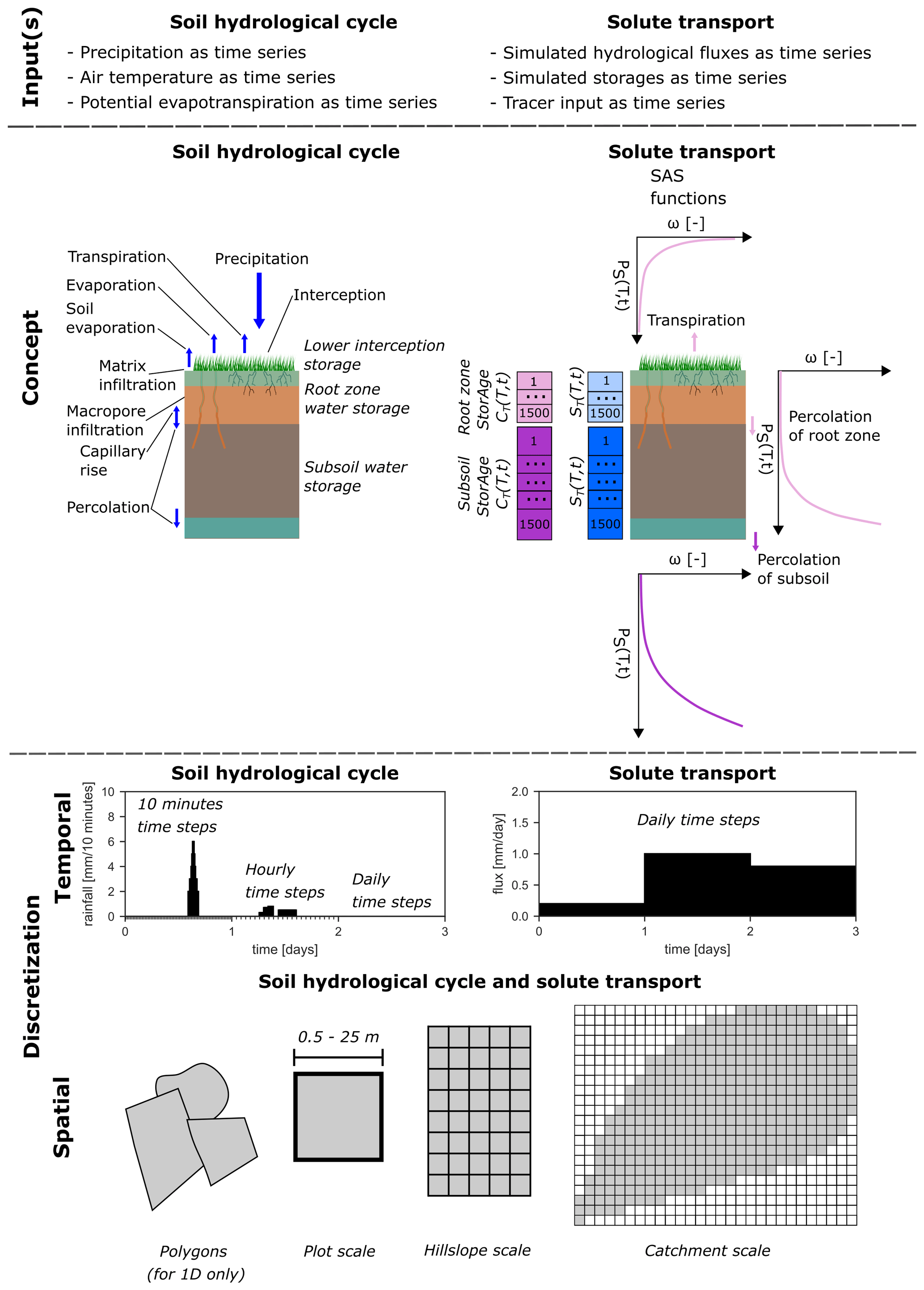
Figure 1 Overview of model inputs, conceptual implementation shown for a single grid cell or unit (water storages are represented in italic), and temporal discretization of the soil hydrological cycle and solute transport. Spatial discretization for different scales is the same for the soil hydrological cycle and solute transport.

RoGeR provides representations for bucket-type interception, degree-day-based snow accumulation and snowmelt (LARSIM-Entwicklergemeinschaft, 2021); soil matrix, macropore and shrinkage crack infiltration (Steinbrich et al., 2016; Weiler, 2005); soil evaporation (Or et al., 2013); vegetation phenology and vegetation-specific transpiration (Steduto et al., 2009); capillary rise from a groundwater table and percolation to the groundwater (Salvucci, 1993); and lateral subsurface runoff (Steinbrich et al., 2016; Stoll and Weiler, 2010). For detailed information (e.g. model equations), we refer the reader to the online documentation of RoGeR (Schwemmle, 2023a).

RoGeR explicitly solves the soil water balance (i.e. fluxes update the state in a specific sequence) using an adaptive time-stepping scheme (see Fig. 1). The adaptive time stepping provides a better compromise between accuracy and performance compared to fixed time-stepping schemes (Clark and Kavetski, 2010). Numerical errors may compensate for model structural errors; we have not evaluated the effect of other time-stepping schemes on the numerical errors in RoGeR. Although numerical errors affect the simulations, parameter uncertainty (e.g. Wagener and Gupta, 2005) or input data uncertainty (e.g. Yatheendradas et al., 2008) may have a stronger impact on the simulations.

2.3 Solute transport model

Solute transport is implemented by a travel-time-based approach. Particularly, we use StorAge selection (SAS) functions (Rinaldo et al., 2015). SAS is implemented by specific distribution functions. We assign a distribution function to each hydrological process (Fig. 1). Here, we introduce two distribution functions which can be used for SAS and are implemented in the toolbox. The first distribution function is based on a power law and requires only a single parameter, k_Q (Fig. 2a). The power law distribution function is given as

$$\begin{array}{}\text{(1)}& {\mathit{\omega }}_Q\left(T,t\right)=k_Q^{k_Q}\cdot P_{\mathrm{s}}{\left(T,t\right)}^{(k_Q-\mathrm{1})},\end{array}$$

with

$$\begin{array}{}\text{(2)}& P_{\mathrm{s}}\left(T,t\right)={\displaystyle \frac{S_T(T,t)}{S\left(t\right)}}\end{array}$$

and the corresponding cumulative power law distribution function:

$$\begin{array}{}\text{(3)}& {\mathrm{\Omega }}_Q\left(T,t\right)=P_{\mathrm{s}}{\left(T,t\right)}^{k_Q},\end{array}$$

where T is the water age (d), t is the time step (d), ω_Q(T,t) is the probability distribution function of the hydrologic flux, Ω_Q(T,t) is the cumulative probability distribution function), S_T(T,t) is the cumulative age-ranked storage (mm), S (t) is the soil water content (mm) and P_s(T,t) is the cumulative probability distribution of the storage.

Figure 2 Storage selection with different parameters, illustrated for the power law distribution function (a; see Eq. 1) and the Kumaraswamy distribution function (b; see Eq. 3).

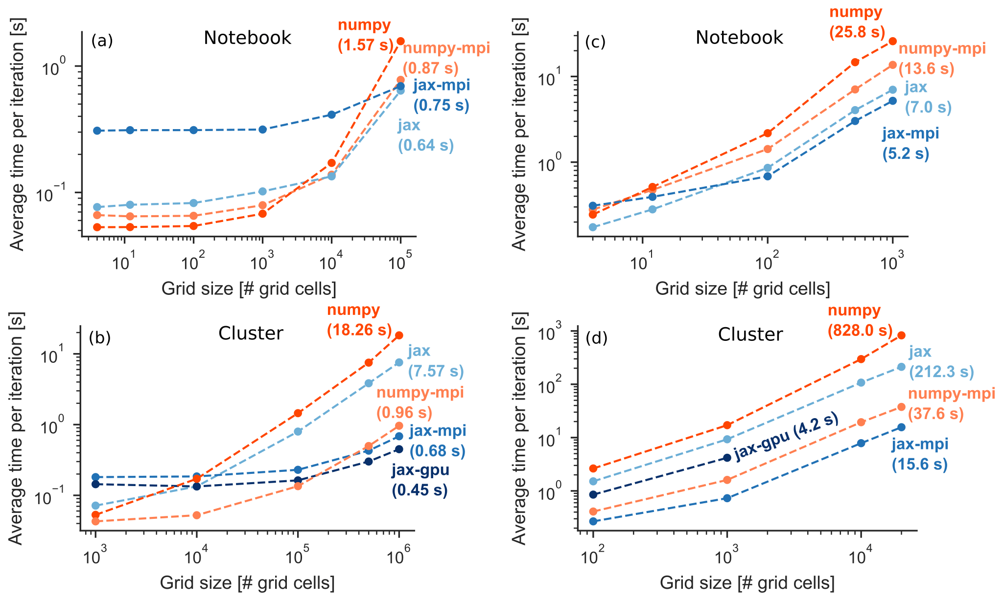
Figure 3 Runtime performance of computational backends for the RoGeR-SVAT-type model (a, b) and for the RoGeR-SVAT-¹⁸O-type transport model (c, d). Note that the number of grid cells represents the two horizontal spatial dimensions (i.e. longitude and latitude). The total number of elements is greater for transport models due to additional age dimensions and can be derived by multiplying the number of grid cells (i.e. two spatial dimensions) by the number of water ages (e.g. 1500). The SVAT model used 100 iterations and the SVAT-¹⁸O transport model used 20 iterations.

Table 2 Hardware specifications of computational benchmarks.

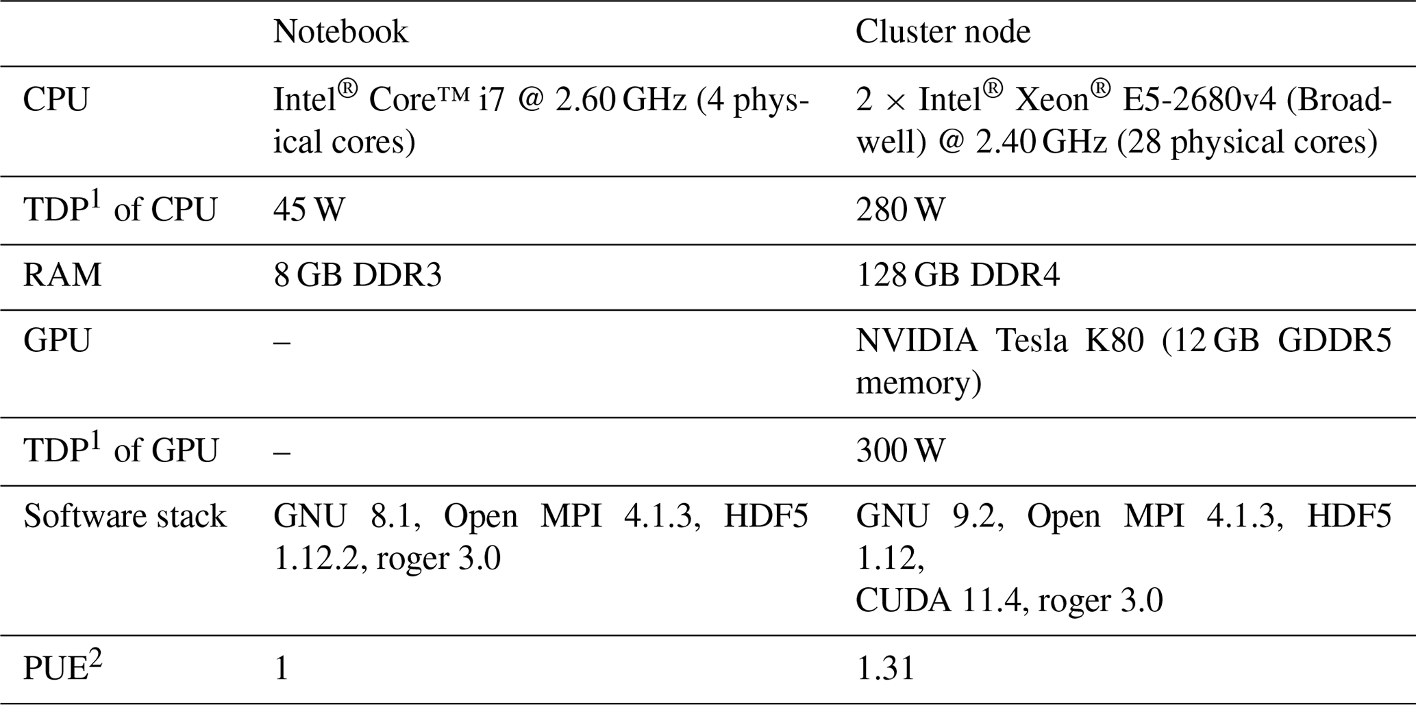
¹ Total power draw. ² Power usage efficiency.

Figure 4 Energy usage of computational backends on a cluster node for the RoGeR-SVAT-type model (a, b) and for the RoGeR-SVAT-¹⁸O-type transport model (c, d).

As a second distribution function, we employ the Kumaraswamy distribution (Kumaraswamy, 1980). With two parameters, a_Q and b_Q, the Kumaraswamy distribution provides a greater flexibility than a power law distribution (Fig. 2b). The Kumaraswamy distribution function is formulated as

$$\begin{array}{}\text{(4)}& {\mathit{\omega }}_Q\left(T,t\right)=a\cdot b\cdot P_{\mathrm{s}}{\left(T,t\right)}^{(a_Q-\mathrm{1})}\cdot \left(\mathrm{1}-P_{\mathrm{s}}{\left(T,t\right)}^{a_Q^{(b_Q-\mathrm{1})}}\right)\end{array}$$

and the corresponding cumulative Kumaraswamy distribution function as

$$\begin{array}{}\text{(5)}& {\mathrm{\Omega }}_Q\left(T,t\right)=\mathrm{1}-\left(\mathrm{1}-{\left(P_{\mathrm{s}}\left(T,t\right)\right)}^{a_Q^{b_Q}}\right).\end{array}$$

Generally, any distribution function might be used as long as a closed form (i.e. probabilities integrated into one) is available (Harman, 2015). We apply the fractional SAS function type (fSAS; van der Velde et al., 2012) and solve the SAS equations for each hydrologic flux, Q. To solve the SAS functions, we provide three numerical schemes with fixed time steps: (i) deterministic (i.e. solving SAS equations for each flux in a sequential order), (ii) explicit Euler and (iii) explicit Runge–Kutta fourth-order. Transport processes can be defined for conservative and non-conservative solutes:

• For stable water isotopes, oxygen-18 (¹⁸O) and deuterium (²H), isotopic fractionation is not yet considered.

• For bromide and chloride, evapoconcentration, sorption processes and partitioning of the root uptake are included.

• For nitrate, biogeochemical process denitrification (Kunkel and Wendland, 2006), nitrification, soil nitrogen mineralization and nitrogen uptake by crops are implemented.

Again, we refer the reader to the online documentation of RoGeR for detailed information (Schwemmle, 2023a). The following routines are implemented, and we refer the reader to the module and declare whether the module is tested or if testing is still ongoing:

• solute transport and water ages (transport.py and sas.py; testing is complete)

• nitrogen cycle (nitrate.py; testing is ongoing).

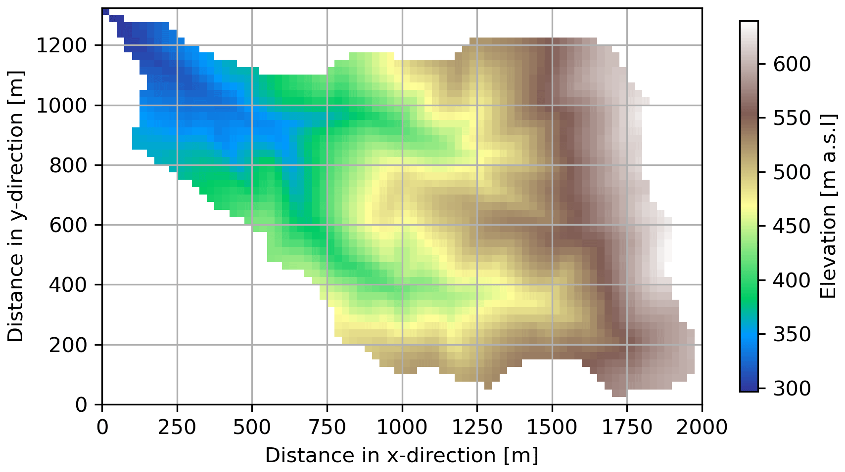
Figure 5 The Eberbaechle catchment used for the application example. Further catchment properties used as model parameters are shown in Figs. S31–S39. The coordinates of the catchment outlet are 47°${\mathrm{57}}^{\prime }{\mathrm{24}}^{\prime \prime }$ N, 7°${\mathrm{49}}^{\prime }{\mathrm{48}}^{\prime \prime }$ E.

Table 3 Model parameters for the Eberbaechle catchment.

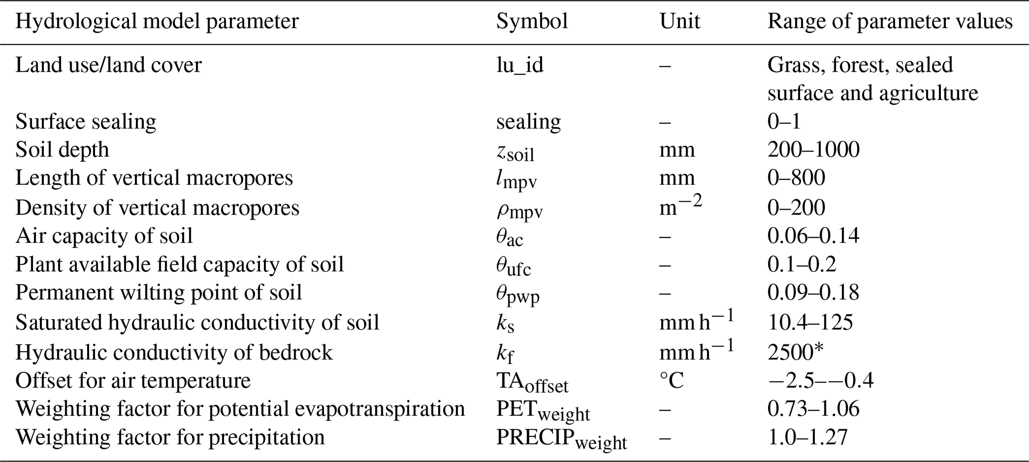
^∗ Parameter value represents free drainage. We assume free drainage since information for the lower boundary condition (i.e. depth of the groundwater table) is not available.

3 Test cases for continuous development, computational performance and energy usage

RoGeR uses unit tests and continuous integration to test and ensure technical functionality (see Table 1). Additionally, we use test cases for continuous development. The idea of these test cases is to guarantee predictive consistency and to track advances in model development (i.e. comparison between model versions). We run the test cases with model parameters that cover a wide range of common parameters and perform simulations with different input data. In contrast to unit tests, the execution time is longer and depends on the number of time steps covered by the input data. The results (see Sect. S1 in the Supplement) can be compared to future versions of RoGeR.

Figure 6 Simulated fluxes and soil water content (a–d); corresponding δ¹⁸O signal (e–h); and corresponding 10th, 50th and 10th percentiles of water ages (i–k) of a single grid cell. Vertical red lines indicate the four different dates from Fig. 7. Power law distribution function serves as a SAS function (SAS parameters are $k_{\mathrm{evap}-\mathrm{soil}}=\mathrm{0.2}$, k_transp=0.5, $k_{\mathrm{kperc}-\mathrm{rz}}=\mathrm{1.5}$, $k_{\mathrm{kperc}-\mathrm{ss}}=\mathrm{1.5}$; see Fig. 2).

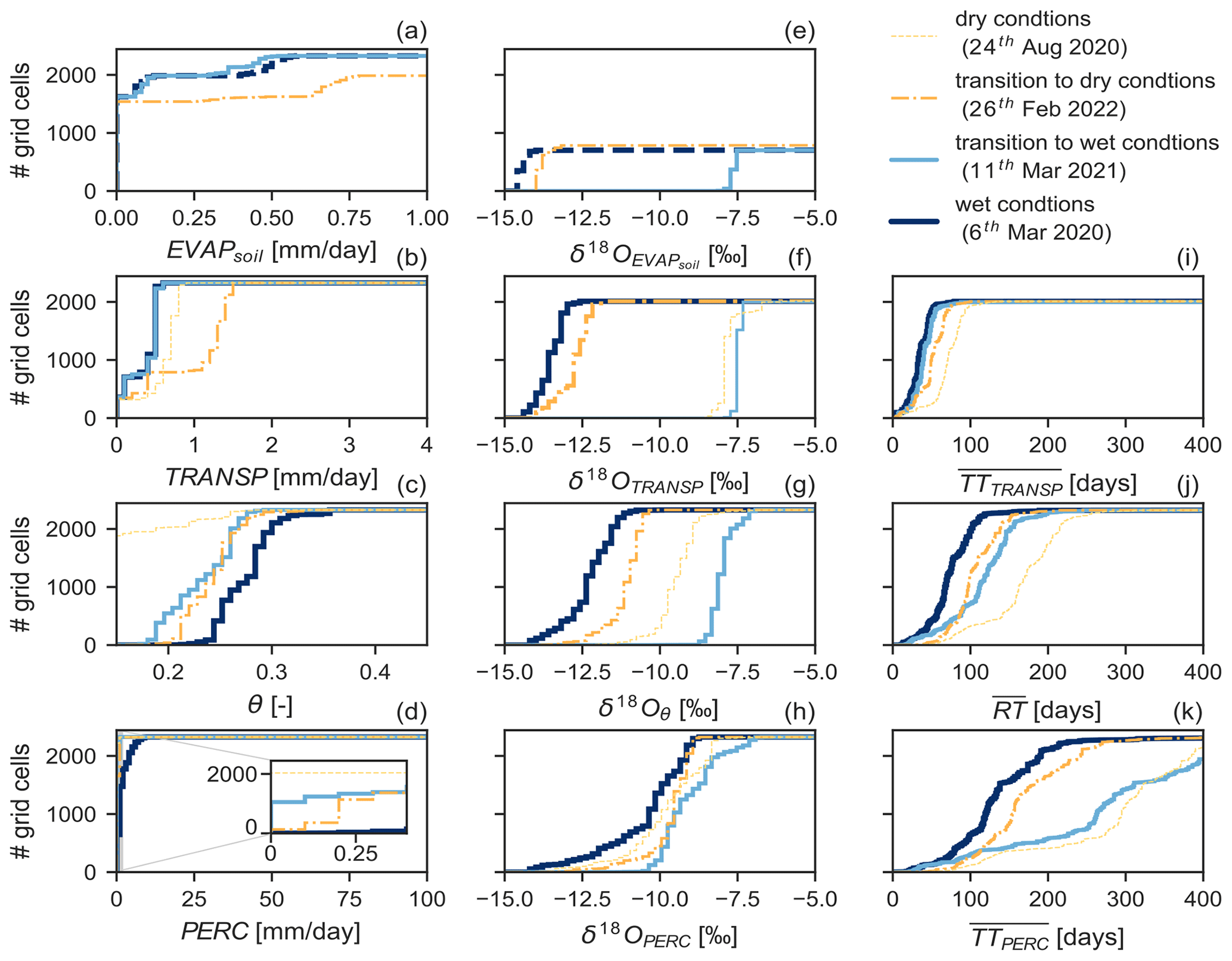
Figure 7 Cumulative distributions of simulated fluxes and soil water content (a–d), corresponding δ¹⁸O signal (e–h), and the corresponding average travel time and average residence time (i–k) of the Eberbaechle catchment (1.54 km²) on four different dates (transition to dry, dry, transition to wet and wet conditions).

High-level programming languages such as Python still have the reputation of being comparatively slow. We profiled the computation time and energy usage using the five backends (see Sect. 2.1.2). For the profiling, we used two different hardware specifications representing commonly available computing resources and high-performance computing (HPC) resources (Table 2). We measured computation time and energy usage with a fixed number of iterations but varying number of grid cells (Fig. 3).

Model parameters are the same for each grid cell. Figure 3 shows that for small modelling experiments (< 1000 grid cells), the numpy backend performs as well as the other backends. Parallel computation improves computational speedup only for intermediate to larger modelling experiments (> 1000 grid cells), provided that a greater number of CPU cores are available. Computation on a single GPU device is faster than on multiple CPUs for the RoGeR-SVAT-type model, while multiple CPUs (numpy-mpi and jax-mpi) are faster than a single GPU device for the RoGeR-SVAT-¹⁸O-type model. However, a major requirement for GPU computing is that the modelling experiment fits into the GPU memory (< 10⁶ grid cells). A solution to the memory limitation would be the usage of multiple GPU devices.

HPC consumes more energy than running computations on a laptop. Depending on the energy source, HPC contributes differently to climate warming (Lannelongue et al., 2021). In order to raise awareness about the energy usage in an HPC context and to provide information for a sustainable allocation of computational resources, we profiled the energy usage of RoGeR in an HPC context (see Table 2). Based on the profiling of computation time, we calculated the energy usage of the five backends using the method proposed by Lannelongue et al. (2021). The results (Fig. 4) show that using multiple CPUs (numpy-mpi and jax-mpi) consumes more energy than other backends. Using a single GPU device decreases energy usage, while computation time still competes with multiple CPUs (cf. Fig. 3). For small and intermediate modelling experiments, single-CPU (numpy and jax) backends use less energy than other backends. With these results, we aim to support efficient and sustainable allocation of computational resources. We suggest that computation time and energy usage should be considered equally for the allocation.

4 Application: soil water balance, ¹⁸O transport and water age statistics of a 3-year period

To demonstrate the capabilities of RoGeR, we present a simple application example. We simulate the soil water balance and fluxes and ¹⁸O fluxes of the Eberbaechle catchment (1.54 km² with a resolution of 25 m × 25 m) for a time period of 3 years. The input data were retrieved from the database WeatherDB, which provides data from stations operated by Deutscher Wetterdienst (DWD), tailored to the required format of RoGeR (Schmit, 2022). We selected the DWD station at Freiburg airport (station ID 1443) to obtain precipitation, air temperature and potential evapotranspiration data from November 2019 to October 2022. Since DWD stations do not measure solute concentrations in precipitation, data for ¹⁸O in precipitation have been generated by a sinusoidal function with random variation for amplitude and offset (Allen et al., 2018; amplitude of 4.3 ± 0.5 ‰, offset of $-\mathrm{10}\pm \mathrm{0.5}$ ‰ and phase of 60 d). In order to set the values for the model parameters listed in Table 3, we used the BK50 soil map (Regierungspräsidium Freiburg, Landesamt für Geologie, Rohstoffe und Bergbau), lidar data (Landesvermessungsamt Baden-Würrtemberg) and ATKIS DLM25 (Landesvermessungsamt Baden-Würrtemberg). Additionally, we assumed a deep groundwater table implemented through a high hydraulic conductivity of the bedrock (see Table 2). SAS parameters for the selected power law distribution function are assumed to be spatially and temporally constant for each hydrological process and grid cell. We assigned k=0.2 to soil evaporation and capillary rise, k=0.5 to transpiration, k=1.5 to percolation of the root zone and k=1.5 to percolation of the subsoil. Thus, soil evaporation capillary rise and transpiration have a preference for younger water, while percolation processes have a preference for older water (see Fig. 2a).

In Fig. 6, we display the time series of hydrologic fluxes and soil water content with the corresponding ¹⁸O signature and water age distributions of a single grid cell. The temporal pattern exhibits that soil water content and travel times of hydrologic fluxes can be related. This pattern emphasizes the interlinkage between hydrologic states and transport velocities of solutes (Hrachowitz et al., 2016). Figure 7 shows the cumulative distributions of soil hydrologic fluxes, soil water content, δ¹⁸O signals and average water ages at four different dates with different soil water content conditions. Soil water content is wetter on 10 February 2021 and drier on 13 August 2022, while the other two dates represent the transition between drier and wetter conditions. The cumulative distributions of δ¹⁸O signals and average water ages reveal differences between these different soil water content conditions. The δ¹⁸O signals display distinct differences between the considered fluxes and soil water storage. The average water age exposes a more general pattern. For drier conditions, average water age is older, whereas for wetter conditions, median water age decreases.

The primary objective of the example is to demonstrate the capabilities of RoGeR. Therefore, we kept the complexity of the example at a simple level. Although a comparison between simulations and observations is important to evaluate the fidelity of the model, we do not provide such a comparison here. Instead, we refer the reader to Schwemmle and Weiler (2023) for an in-depth evaluation of RoGeR using measurements from a grassland lysimeter site. Since the development of RoGeR as scientific software started recently and is still ongoing, further evaluation of RoGeR will be made in the future.

The simple application example demonstrates the potential of RoGeR for a combined quantification of the water balance and solute mass balance. The example focuses on vertical soil hydrological processes and a conservative tracer, but this is just an excerpt from the toolbox. Other processes (e.g. lateral subsurface runoff and a different SAS function; see Sect. 2.2 and 2.3) or other tracers (e.g. bromide; see Sect. 2.3) could also be considered and implemented.

5 Summary and outlook

The development of the process-based hydrological toolbox RoGeR followed open-source software guidelines (Sect. 2.1). We believe that such guidelines improve the reproducibility in computational hydrology. With the modular code structure (Sect. 2.1.1) and the good readability of Python code, RoGeR is intended to be easy to use (i.e. usable by programmers with little experience) and to be easy to modify (i.e. modification and extension of the code). With using different computational backends, we maintained code readability without hampering computational performance (Sect. 2.1.2). The five backends provide the opportunity to simulate anything between plot scale and the catchment scale with reasonable computation times. Especially, the GPU backend has great potential for reducing computation time and energy usage of catchment-scale modelling experiments (Sect. 3).

In comparison to the publicly available hydrological models written in Python, we combined hydrological processes (Sect. 2.2) and solute transport based on SAS (Sect. 2.3). The combined representation enables the prediction of hydrologic states and fluxes and their corresponding solute concentrations, including travel times. The simple application example considering the water balance and ¹⁸O transport through the soil of the Eberbaechle catchment showed plausible results. The RoGeR toolbox contains many processes to describe one-dimensional hydrological processes (i.e. no lateral transfer between grid cells). The implementation of the lateral transfer between grid cells (i.e. routing schemes for surface and subsurface runoff) will be addressed in future releases. Surface runoff routing will be implemented using a hydraulic scheme. Subsurface runoff routing will use the approach of Steinbrich et al. (2016), which is based on the topographic slope and corresponding flow velocities. Moreover, we suggest that future work may improve or extend the currently available process representations (e.g. gravity-driven infiltration and percolation; Demand and Weiler, 2021; Germann and Prasuhn, 2018) and further evaluation of RoGeR with measured data may provide insights into the strengths and weaknesses.

RoGeR contributes to a further diversification of the hydrological model landscape, and the disagreement about process representation in the hydrological modelling community will continue (Weiler and Beven, 2015). In general, an advantage of this diversification and disagreement is that many different approaches and, hence, a great flexibility to address different problems are available. On the other hand, the theoretical diversification is accompanied by technical diversification (e.g. different programming languages or different data formats) that leads to inconsistencies in the application. We suggest that the diverse hydrological model landscape might benefit from focusing on constrained data interfaces of the models following common data conventions (Hallouin et al., 2022) and implementing standardized model interfaces (Hut et al., 2022; Hutton et al., 2020). This would facilitate the coupling of hydrological models with other models (e.g. groundwater models). Another advantage would be that multiple hydrological models could be compared more easily. Such a model comparison of RoGeR with other models – for example, with tRIBS (Ivanov et al., 2004a, b; Vivoni et al., 2004), DHSVM (Wigmosta et al., 1994) or mHM (Samaniego et al., 2010) – may be useful to highlight the advantages and disadvantages of using RoGeR compared to other models.