Automatic adjoint-based inversion schemes for geodynamics: reconstructing the evolution of Earth's mantle in space and time

Reconstructing the thermo-chemical evolution of Earth's mantle and its diverse surface manifestations is a widely recognised grand challenge for the geosciences. It requires the creation of a digital twin: a digital representation of Earth's mantle across space and time that is compatible with available observational constraints on the mantle's structure, dynamics and evolution. This has led geodynamicists to explore adjoint-based approaches that reformulate mantle convection modelling as an inverse problem, in which unknown model parameters can be optimised to fit available observational data. Whilst there has been a notable increase in the use of adjoint-based methods in geodynamics, the theoretical and practical challenges of deriving, implementing and validating adjoint systems for large-scale, non-linear, time-dependent problems, such as global mantle flow, has hindered their broader use. Here, we present the Geoscientific ADjoint Optimisation PlaTform (G-ADOPT), an advanced computational modelling framework that overcomes these challenges for coupled, non-linear, time-dependent systems by integrating three main components: (i) Firedrake, an automated system for the solution of partial differential equations using the finite-element method; (ii) Dolfin-Adjoint, which automatically generates discrete adjoint models in a form compatible with Firedrake; and (iii) the Rapid Optimisation Library, ROL, an efficient large-scale optimisation toolkit; G-ADOPT enables the application of adjoint methods across geophysical continua, showcased herein for geodynamics. Through two sets of synthetic experiments, we demonstrate the application of this framework to the initial condition problem of mantle convection, in both square and annular geometries, for both isoviscous and non-linear rheologies. We confirm the validity of the gradient computations underpinning the adjoint approach, for all cases, through second-order Taylor remainder convergence tests and subsequently demonstrate excellent recovery of the unknown initial conditions. Moreover, we show that the framework achieves theoretical computational efficiency. Taken together, this confirms the suitability of G-ADOPT for reconstructing the evolution of Earth's mantle in space and time. The framework overcomes the significant theoretical and practical challenges of generating adjoint models and will allow the community to move from idealised forward models to data-driven simulations that rigorously account for observational constraints and their uncertainties using an inverse approach.

1 Introduction

Mantle convection is the “engine” driving our dynamic planet. It is the principal control on Earth's thermal and chemical evolution and underpins tectonic and geological activity at Earth's surface (e.g. Davies and Richards, 1992; Coltice et al., 2017). Through interactions with Earth's crust, it introduces heat and fluids that contribute to the formation and concentration of ore deposits (e.g. Hoggard et al., 2020). Mantle flow also induces vertical movements of Earth's surface (so-called dynamic topography; see Davies et al., 2023, for a review), leading to regional and global changes in sea level and climate (e.g. Poore et al., 2006; Moucha et al., 2008; Cloetingh and Haq, 2015). The lithosphere, considered here to be the mantle's upper thermal boundary layer, serves as a window into the form and time-dependence of mantle convection, recorded through tectonic plate motions (e.g. Iaffaldano and Bunge, 2015; Müller et al., 2016; Stotz et al., 2017, 2018; Wang et al., 2023). Although substantial progress has been made in reconstructing the history of plate tectonic motions (e.g. Seton et al., 2012; Gurnis et al., 2012; Müller et al., 2019; Merdith et al., 2021), the quest for a dynamic reference, revealing the force equilibria within the underlying mantle, remains ongoing. In other words, the veracity of plate motion reconstructions is not matched by an equivalent knowledge of the thermo-chemical structure and flow history of the underlying mantle. This is a major limitation, as it inhibits our ability to understand fundamental processes that depend on time-dependent interactions between Earth's surface and its deep interior.

The primary challenge in reconstructing past mantle flow stems from the lack of knowledge surrounding the initial state, compounded by uncertain physical and chemical parameters. Mantle convection is an initial condition problem, uniquely determined by an initial condition some time in the past: starting from some point in time, it can be uniquely modelled by solving conservation equations for mass, momentum and energy (e.g. Ricard, 2007; Zhong et al., 2007). However, the lack of knowledge on this initial condition – specifically the thermo-chemical state of Earth's mantle at some time in the past – renders reconstructions of mantle flow through conventional forward calculations intractable (Bunge et al., 2003) (Fig. 1a). Moreover, current global mantle convection models employ billions of degrees of freedom and require multiple time steps to resolve the multi-scale dynamics of Earth's mantle (e.g. Davies and Davies, 2009; Wolstencroft et al., 2009; Stadler et al., 2010; Weismüller et al., 2015; Dannberg and Gassmöller, 2018; Bauer et al., 2019, 2020). Owing to the resulting computational expense, the use of conventional geophysical inverse methods, including Monte Carlo techniques (e.g. Sambridge and Mosegaard, 2002), is considered impractical for determining the mantle's past structure, dynamics and evolution.

The initial condition problem can be partially addressed through sequential data-assimilation techniques. In essence, the objective of sequential data assimilation is to leverage all accessible information to improve predictions of mantle flow in space and time. Data assimilation is commonly achieved through sequential filtering (e.g. Wunsch, 1996), in which the model is advanced in time over the period in which observations exist. Whenever observations become available, the model is adjusted or “corrected” (e.g. Bunge and Grand, 2000; Bocher et al., 2016). The magnitude of the correction can be optimally determined using methods such as the Kalman filter (e.g. Bocher et al., 2018), with the model subsequently restarted from the updated state, and this process is repeated until all available information has been utilised (Fig. 1b). In a geodynamic context, the most commonly exploited dataset consists of palaeo-surface velocities from plate tectonic reconstruction models, primarily through a kinematic surface boundary condition in time-dependent models. In recent years, there has been a notable increase in the use of this approach (e.g. Bunge et al., 2002; Davies et al., 2012; Bower et al., 2013; Zhong and Rudolph, 2015; Nerlich et al., 2016; Young et al., 2022; Panton et al., 2023). This can be attributed to two main factors: (i) improved confidence in the validity of plate tectonic reconstruction models and their extension further back in time (e.g. Merdith et al., 2021; Young et al., 2022; Müller et al., 2022) and (ii) the enhanced accessibility of such models, facilitated via open-source community frameworks like the GPlates project (e.g. Gurnis et al., 2012; Müller et al., 2018).

Sequential data-assimilation methods, however, come with an inherent limitation: due to the sequential nature of the assimilation process, each observation is incorporated to influence the model only at later times. Consequently, information propagates from the past into the future but cannot be transmitted back into the past. This drawback poses a significant limitation, as our knowledge of the mantle at the present day is substantially more detailed than at any other time. Thus, it becomes imperative to explore approaches that explicitly carry information backwards in time, or more precisely, enable the estimation of a time-dependent model that best fits all available observational constraints.

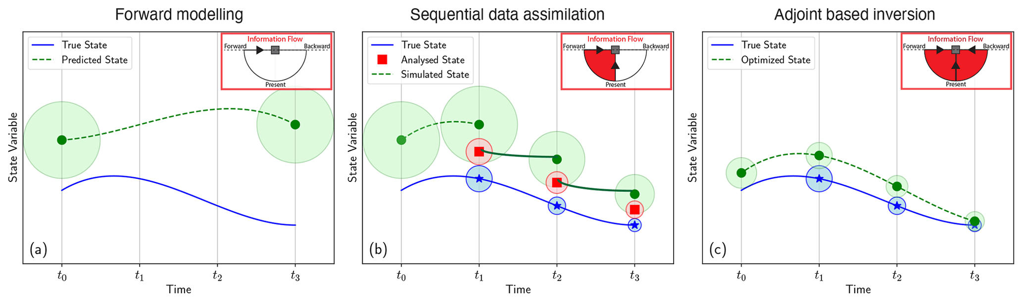
Figure 1 Illustration of different procedures available for estimating past mantle structure: (a) forward modelling prediction, where an unknown initial condition is estimated at t₀, with modelling error measured as the difference between the modelled and true states. This difference is represented by the distance along the y axis, which typically grows in time. Variations in forward modelling include “nudging” of the initial condition to better match present-day structure; (b) sequential data assimilation or “Kalman filtering” – starting from an initial condition at t₀, the forward model is run until t₁. An analysis is subsequently undertaken from the resulting model and the available observation. The corrected model is then subsequently integrated in time until t₂, when the next observation is available. This process is repeated until t₃ or the last time step with available observational data. The information flow diagram depicts how information is carried from both the past and present, using current data; (c) adjoint-based or 4-D variational data assimilation, which is capable of carrying information on present-day structure (e.g. images from seismic tomography) explicitly backward in time. In (c) observational data that constrain present-day mantle structure, alongside data from different points in space and time, are used to optimise the unknown initial condition. Here, all available observations between t₃ and t₀ contribute to the analysis. The true (unknown) signal is represented by the solid line. Observations (stars), predictions (dark circles) and analyses (squares) are surrounded by ellipsoids of a size proportional to the estimated model uncertainty. Modified from Carrassi et al. (2018) and Davies et al. (2023).

Inverse geodynamics is a rapidly evolving field that embarks on this very idea. The foundation of this field is an optimisation approach, in which mantle convection modelling is reformulated as an inverse problem. Using inverse theory, unknown model parameters can be optimised to fit available observational data via the so-called adjoint method (e.g. Bunge et al., 2003; Ismail-Zadeh et al., 2004), through which the sensitivities of a performance measure (the so-called “objective functional”), with respect to model parameters (e.g. the choice of initial condition), can be computed. The resulting sensitivity information can be used to adjust model parameters, generating a model flow trajectory that matches observational constraints (e.g. present-day mantle thermo-chemical structure) (Fig. 1c). The geodynamic adjoint equations for reconstructing the initial condition have been derived for isochemical, incompressible (e.g. Bunge et al., 2003; Horbach et al., 2014), compressible (Ghelichkhan and Bunge, 2016) and thermo-chemical mantle flow (Ghelichkhan and Bunge, 2018). Moreover, the method has been enhanced for simultaneous recovery of initial temperature conditions and rheological parameters (Li et al., 2017) despite the inherent ill-posedness introduced in such a problem. Growing adoption of adjoint-based methods within a broader geodynamic context is evidenced by their application in Reuber et al. (2020) to decipher subsurface structures and rheological parameters via inversion of principal stress directions and by Crawford et al. (2018) to quantify the sensitivity of post-glacial sea level changes to lateral variations in mantle viscosity. Recent growth in computational power has led to multiple adjoint-based mantle reconstructions, with a particular focus on regional geological events, as recorded in the geological record of the Americas (e.g. Spasojevic et al., 2009; Liu and Gurnis, 2010; Shephard et al., 2010) and the Atlantic realm (e.g. Colli et al., 2018). To supplement these findings, Ghelichkhan et al. (2021) undertook a systematic global-scale comparison between adjoint model predictions and independent geological constraints, with implications for the expected rates of gravitational and dynamic ellipticity changes resulting from convection within Earth's mantle (Ghelichkhan et al., 2018, 2020).

While substantial strides have been made in the application of adjoint-based methods in geodynamics, there remain widespread obstacles to the broader use of these techniques within the geodynamic modelling community. One key challenge is the complexity involved with deriving, implementing and validating adjoint models for large-scale, non-linear, time-dependent problems, core features of global mantle convection models. Owing to these difficulties, studies that have used the adjoint method to explore the thermo-chemical evolution of Earth's mantle often resort to a simplified strategy. This typically involves either a highly idealised treatment of mantle rheology (e.g. Colli et al., 2018; Ghelichkhan et al., 2021), omitting certain coupling terms in the adjoint equations, or doing both (e.g. Liu et al., 2008; Spasojevic et al., 2009; Liu and Gurnis, 2010; Shephard et al., 2010). Such simplifications limit the applicability of these results. The work of Li et al. (2017) is a notable exception to this trend, although its focus on a 2-D rectangular domain, specifically aimed at reconstructing the dynamics of subduction, inherently limits its applicability to global mantle convection simulations. Furthermore, previous global applications of the adjoint approach have been hampered by their reliance on legacy community codes (e.g. Bunge et al., 2003; Liu et al., 2010; Shephard et al., 2010; Colli et al., 2018; Ghelichkhan et al., 2021). These codes are not easily extensible to different geometries or approximations of the underlying physics, employ solver strategies that have since been superseded, and often have limits on model resolution due to the fully structured discretisations encoded. Moreover, the complex and extensive low-level code implementation of coupled adjoint and forward calculations remains obscured, making it difficult to extend and validate, thus restricting the types of observational datasets that can be incorporated. An example of these datasets are the (uncertain) constraints provided by plate tectonic reconstruction models that are prescribed kinematically (e.g. Spasojevic et al., 2009; Shephard et al., 2010; Zhou and Liu, 2017; Colli et al., 2018; Ghelichkhan et al., 2021) as opposed to being formally incorporated through the objective functional. The kinematic prescription of the surface velocities, however, can only improve mantle reconstructions forward in time and therefore prohibits their influence on previous system states. In light of these limitations, there is a need for a general framework that can robustly handle the rheological complexities of Earth's mantle and is easily extensible and transferable to other problems in mantle and lithosphere dynamics. Such a framework must also be capable of utilising a variety of observational constraints to comprehensively unravel the historical evolution of Earth's interior and its diverse impacts at Earth's surface  (Davies et al., 2023).

In this paper, we introduce the Geoscientific ADjoint Optimisation PlaTform (G-ADOPT), research software infrastructure that allows us to overcome these limitations. G-ADOPT is built around three state-of-the-art software libraries – (i) Firedrake, an automated system for solving a range of partial differential equations using the finite-element method (Rathgeber et al., 2016), recently validated for geodynamics (Davies et al., 2022); (ii) Dolfin-Adjoint, which automatically derives the discrete adjoint equations in a form compatible with Firedrake (Farrell et al., 2013a; Mitusch et al., 2019); and (iii) the Rapid Optimisation Library (ROL), a Trilinos package for performing highly efficient large-scale optimisation (The ROL Project Team, 2022). When combined, they provide a geodynamic inversion framework that is highly efficient, with fully consistent forward and adjoint calculations that achieve theoretical computational efficiency.

We structure our paper as follows: in Sect. 2.1 we describe the geodynamic forward problem and our solution strategy using G-ADOPT. Section 2.2 describes the inverse problem considered herein, where we focus on finding the (unknown) initial condition using an objective functional that accounts for observations of surface velocity over time and the final state temperature field. This is broken into three subsections: (i) Sect. 2.2.1 describes discrete and continuous approaches for obtaining the adjoint systems followed by a detailed derivation of the discrete adjoint systems; (ii) Sect. 2.2.2 introduces Dolfin-Adjoint, the underlying approach utilised in G-ADOPT to compute the discrete adjoint and derivative fields; and (iii) Sect. 2.2.6 provides an overview of the gradient-based optimisation approach utilised here, facilitated by ROL. We demonstrate the applicability of our approach in Sect. 3 using two sets of twin experiments with increasing complexity, where we reconstruct the spatial and temporal evolution of a reference simulation. The first set of experiments (Sect. 3.1) involves a simple isoviscous simulation within an enclosed square domain, while the second set (Sect. 3.2) examines convection with a non-linear (temperature, depth and strain rate dependent) rheology at Earth-like convective vigour within an annular domain, which has direct applicability to convection within Earth's mantle. We finish by discussing our results and conclusions in Sects. 4 and 5, respectively.

2 Method

2.1 Forward problem

2.1.1 Governing equations and boundary conditions

Mantle flow is described by conservation laws for mass, momentum and energy. We solve these equations in their simplest form, assuming incompressibility and the Boussinesq approximation. The three non-dimensional conservation equations are

$$\begin{array}{}\text{(1a)}& {\displaystyle }-\mathrm{\nabla }\cdot \left(\mathrm{2}\mathit{\eta }\dot{\mathit{ϵ}}\left(\mathit{u}\right)\right)+\mathrm{\nabla }p+\mathit{Ra}T\widehat{\mathit{k}}& {\displaystyle }=\mathrm{0},\text{(1b)}& {\displaystyle }\mathrm{\nabla }\cdot \mathit{u}& {\displaystyle }=\mathrm{0},\text{(1c)}& {\displaystyle \frac{\partial T}{\partial t}}+\mathit{u}\cdot \mathrm{\nabla }T-\mathit{\kappa }{\mathrm{\nabla }}^{\mathrm{2}}T-H& {\displaystyle }=\mathrm{0},\end{array}$$

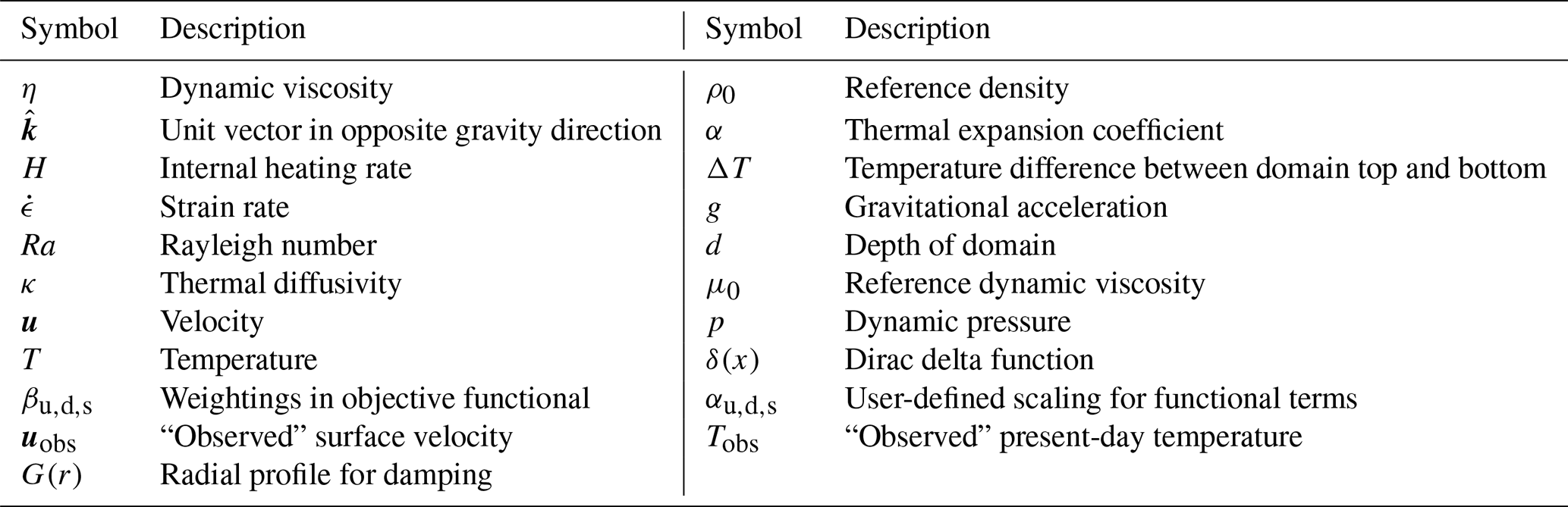
with the vector field u and scalar fields p and T as the principal unknowns of velocity, pressure and temperature, respectively. Table 1 summarises other symbols used in Eqs. (1a)–(1c) and elsewhere. In Eq. (1a), the strain-rate tensor $\dot{\mathit{ϵ}}\left(\mathit{u}\right)$ is given by

$$\begin{array}{}\text{(2)}& {\displaystyle }\dot{\mathit{ϵ}}\left(\mathit{u}\right)={\displaystyle \frac{\mathrm{1}}{\mathrm{2}}}\left(\mathrm{\nabla }\mathit{u}+(\mathrm{\nabla }\mathit{u}{)}^T\right),\end{array}$$

and the Rayleigh number is defined by

$$\begin{array}{}\text{(3)}& {\displaystyle }\mathit{Ra}={\displaystyle \frac{{\mathit{\rho }}_{\mathrm{0}}\mathit{\alpha }\mathrm{\Delta }Tg{d}^{\mathrm{3}}}{{\mathit{\mu }}_{\mathrm{0}}\mathit{\kappa }}}.\end{array}$$

For this problem, we define the time interval of interest as $I=[t_{\mathrm{I}},t_{\mathrm{F}}]$, with the computational domain V bounded by ∂V, and S and C denoting the top and bottom boundaries, respectively. For all simulations, free-slip and impermeable velocity boundary conditions are specified on all boundaries, whilst temperature boundary conditions are set to constant values of T_S and T_C at top and bottom boundaries, respectively. For the simulations considered in an enclosed square domain, natural temperature boundary conditions (zero heat flux) are specified on side walls. The set of boundary conditions, for top and bottom boundaries, are listed in Eqs. (4a)–(4d):

$$\begin{array}{}\text{(4a)}& {\displaystyle }\mathit{u}(x,t)\cdot \mathit{n}& {\displaystyle }=\mathrm{0},& {\displaystyle }x\in \partial V,t\in I,\text{(4b)}& {\displaystyle }\left[\mathit{\eta }\dot{\mathit{ϵ}}\left(\mathit{u}\left(x,t\right)\right)\cdot \mathit{n}\right]\cdot \mathit{s}& {\displaystyle }=\mathrm{0},& {\displaystyle }x\in \partial V,t\in I,\text{(4c)}& {\displaystyle }T(x,t)& {\displaystyle }=T_{\mathrm{S}},& {\displaystyle }x\in S,t\in I,\text{(4d)}& {\displaystyle }T(x,t)& {\displaystyle }=T_C,& {\displaystyle }x\in C,t\in I.\end{array}$$

In Eqs. (4a)–(4d), n denotes the outer normal vector and s any tangential vector. Finally, as mantle convection is an initial value problem, we require a prescribed temperature field at initial time t_I:

$$\begin{array}{}\text{(5)}& {\displaystyle }T(x,t_{\mathrm{I}})=T_{\mathrm{IC}}\left(x\right),x\in V.\end{array}$$

Table 1 Symbols used in this study.

2.1.2 Solution strategy: leveraging Firedrake through G-ADOPT

We use the finite-element method to solve the coupled system of partial differential equations presented in Eqs. (1a)–(1c). For the Stokes system, we use a Q₂−Q₁ (piecewise biquadratic and bilinear, respectively) finite-element pair for velocity and pressure, with Q₂ elements used for temperature. We strongly impose Dirichlet boundary conditions for temperature at top and bottom boundaries. Free-slip velocity boundary conditions are imposed in two ways: (i) in our square domain cases, we impose strong Dirichlet boundary conditions for u; (ii) in our annular domain cases, where boundaries do not align with Cartesian directions, we employ a symmetric Nitsche penalty method (Nitsche, 1971), which weakly enforces boundary conditions via a modification of the variational formulation. An implicit mid-point scheme is used for time integration in the energy equation.

To solve the coupled system of forward (and adjoint) equations, we employ Firedrake, which provides an automated system designed for the solution of partial differential equations using the finite-element method (Ham et al., 2023). It incorporates principles and some aspects of the code-base from the FEniCS project (Logg et al., 2012), including its use of the Unified Form Language (UFL) (Alnæs et al., 2014) for the representation of variational problems. UFL is a high-level language utilised for the symbolic description of the governing equations in a form that closely mimics their mathematical formulation. The key advantage of UFL in this work lies in its high-level abstraction, which allows for an innovative automatic derivation approach when deriving adjoint systems. We will address the significance of UFL in automatic derivation of adjoint systems in Sect. 2.2.2.

Firedrake provides an array of features that are particularly conducive to tackling problems in geophysical fluid dynamics. Key among these features is support for a variety of finite-element discretisations, including a highly efficient implementation of discretisations based on extruded meshes; programmable non-linear solves; and operator-aware solver preconditioners that can be combined in a flexible manner to create linear or non-linear systems, which are solved by PETSc (e.g. Balay et al., 1997; Dalcin et al., 2011; Balay et al., 2023). The suitability of Firedrake for geodynamics has been demonstrated via comparison with a comprehensive set of analytical solutions and community benchmarks in Davies et al. (2022). We refer the reader to this study, alongside Rathgeber et al. (2016), for a more in-depth discussion on Firedrake and its dependencies, alongside an outline of the solution strategy employed herein.

Building upon the foundations provided by Firedrake, G-ADOPT introduces an array of features tailored for cutting-edge geodynamical simulations. It integrates smoothly with Firedrake's advanced data-loading capabilities, enabling finite-element consistent point-data interpolation (Nixon-Hill et al., 2023) and facilitating the integration of diverse observational and physical datasets. Various non-linear rheological laws can be effortlessly incorporated using the symbolic representation provided by UFL. G-ADOPT provides a selection of time discretisation schemes, including second-order Runge–Kutta and backward/forward Euler methods. Visualisation capabilities are provided through integration with the “Visualization Toolkit” (VTK), allowing comprehensive analysis in ParaView, among other visualisation packages. Compatibility with meshes generated by gmsh and seamless integration with NETGEN provide straightforward support for a range of mesh configurations and adaptive mesh refinement. G-ADOPT offers a diverse array of boundary conditions, encompassing free- and no-slip conditions, a free-surface (Kramer et al., 2012), and kinematic forcing, for example, via seamless integration with pyGPlates (Gurnis et al., 2012; Müller et al., 2018). The collection of features, elaborately detailed in the Firedrake and G-ADOPT online documentation and referenced in Davies et al. (2022), highlights the platform's robustness and adaptability for geodynamical research.

2.2 Inverse problem: an optimisation approach

Representative reconstructions of the spatial and temporal evolution of mantle flow require knowledge of the initial condition (i.e. the thermo-chemical state of the mantle at some point in the past), the determination of which is an inverse problem. We therefore seek the best-fitting initial condition (T_IC) that results in the minimum of an objective functional that measures the difference between predictions and observations of mantle states and irregularity in the solutions. We use the following mathematical description of the objective functional:

$$\begin{array}{}\text{(6)}& \begin{array}{rl}J=& {\displaystyle \frac{\mathrm{1}}{\mathrm{2}}}\underset{I}{\int }\underset{V}{\int }{\left(T-T_{\mathrm{obs}}\right)}^{\mathrm{2}}\mathit{\delta }(t-t_{\mathrm{F}})\mathrm{d}x\mathrm{d}t\\ +{\displaystyle \frac{{\mathit{\beta }}_{\mathrm{u}}}{\mathrm{2}}}& \underset{I}{\int }\underset{S}{\int }\left(\mathit{u}-{\mathit{u}}_{\mathrm{obs}}\right)\cdot \left(\mathit{u}-{\mathit{u}}_{\mathrm{obs}}\right)\mathrm{d}s\mathrm{d}t\\ +{\displaystyle \frac{{\mathit{\beta }}_{\mathrm{d}}}{\mathrm{2}}}& \underset{I}{\int }\underset{V}{\int }G\left(r\right){\left(T-\overline{T}\right)}^{\mathrm{2}}\mathit{\delta }(t-t_{\mathrm{I}})\mathrm{d}x\mathrm{d}t\\ +{\displaystyle \frac{{\mathit{\beta }}_{\mathrm{s}}}{\mathrm{2}}}& \underset{I}{\int }\underset{V}{\int }{\left[\mathrm{\nabla }\left(T-\overline{T}\right)\right]}^{\mathrm{2}}\mathit{\delta }(t-t_{\mathrm{I}})\mathrm{d}x\mathrm{d}t.\end{array}\end{array}$$

The first term in Eq. (6) accounts for the misfit between model predictions and temperature recorded at the final instance, whilst the second term measures the misfit in surface velocities through time. The other terms are Tikhonov regularisation components (Tikhonov, 1963; Hansen, 1992), the first of which penalises deviations from an a priori depth-averaged profile, $\overline{T}$ (i.e. the damping term), and the second penalises the gradient of these deviations to produce less complex solutions (i.e. the smoothing term). For the damping term, we employ a depth-dependent pre-factor, G(r), that is zero within the mid-mantle but transitions to one in the thermal boundary layers. In these areas, lateral material transport and diffusive processes dominate, leading to diminished sensitivity between the choice of initial condition and the final temperature field. G(r), therefore, helps to minimise the amplitude of the solution within the top and bottom thermal boundary layers, removing noise that would otherwise diffuse over the simulation. The three weighting terms, β_u, β_s and β_d, in Eq. (6) are defined as

$$\begin{array}{}\text{(7a)}& {\displaystyle }{\mathit{\beta }}_{\mathrm{u}}& {\displaystyle }={\mathit{\alpha }}_{\mathrm{u}}{\displaystyle \frac{\underset{V}{\int }{T}_{\mathrm{obs}}^{\mathrm{2}}\mathrm{d}x}{\mathrm{\Delta }t\underset{S}{\int }\left({\mathit{u}}_{\mathrm{obs}}^{t=t_{\mathrm{F}}}\cdot {\mathit{u}}_{\mathrm{obs}}^{t=t_{\mathrm{F}}}\right)\mathrm{d}x}},\text{(7b)}& {\displaystyle }{\mathit{\beta }}_{\mathrm{d}}& {\displaystyle }={\mathit{\alpha }}_{\mathrm{d}}{\displaystyle \frac{\underset{V}{\int }{T}_{\mathrm{obs}}^{\mathrm{2}}\mathrm{d}x}{\underset{V}{\int }{\left(\overline{T}\right)}^{\mathrm{2}}\mathrm{d}x}},\text{(7c)}& {\displaystyle }{\mathit{\beta }}_{\mathrm{s}}& {\displaystyle }={\mathit{\alpha }}_{\mathrm{s}}{\displaystyle \frac{\underset{V}{\int }{T}_{\mathrm{obs}}^{\mathrm{2}}\mathrm{d}x}{\underset{V}{\int }{\left(\mathrm{\nabla }\overline{T}\right)}^{\mathrm{2}}\mathrm{d}x}}.\end{array}$$

Note that Δt is the total duration of the simulation. The integrals in Eqs. (7) are employed to ensure normalised objective terms relative to the final temperature misfit (first term on the right-hand side of Eq. 6). The three scaling parameters, α_u, α_s and α_d, can be set to adjust the importance of these terms relative to the final temperature misfit. We perform a parameter search to find the best-performing combinations of α values.

For our inverse problem we are interested in optimising J described by Eq. (6). J depends on some “control” parameters, which in this case is the initial temperature field, and some “state” variables (i.e. surface velocity and the final temperature), which are solutions of the forward problem in Eqs. (1a)–(1c), with the forward system itself depending again on the control. To solve this problem, we define a “reduced” functional, which is a function of the initial condition, T_IC, alone. This reduced functional is typically defined by first solving the forward partial differential equations (PDEs) (Eqs. 1a–1c) for a given value of the control and then substituting the solutions into the expression for the functional (Eq. 6). The result is a functional that depends only on the control parameters, not the state variables directly (hence the name reduced).

Non-linear optimisation methods provide the means to find the optimal T_IC by minimising a reduced functional defined by J. These methods are iterative. They begin with an initial guess of T_IC to generate a sequence of improved estimates (called iterates) until certain conditions, e.g. residual tolerance, in the objective functional are achieved. Crucial for the efficiency of these iterations are derivatives of Eq. (6) with respect to T_IC. Owing to the large number of unknowns in 3-D spherical mantle convection models with Earth-like parameters, obtaining the derivative by means of classical finite differencing techniques is impractical. The adjoint method serves as a mathematically elegant and computationally efficient way to obtain the derivatives (e.g. Talagrand, 1997; Giles and Pierce, 2000; Plessix, 2006; Hinze et al., 2008).

2.2.1 Continuous versus discrete adjoints

Approaches to deriving, implementing and obtaining derivatives using the adjoint method primarily fall into two categories: (i) continuous, or the differentiate-then-discretise approach, and (ii) discrete, or the discretise-then-differentiate approach (Gunzburger, 2000).

The continuous approach commences with the derivation of the adjoint equations. The resemblance between the forward and resulting adjoint equations allows the adjoint PDEs to be discretised in a consistent manner and, subsequently, implemented within a numerical framework. By deriving the continuous adjoint PDEs, one can develop an understanding of the key characteristics of adjoint sensitivities, the physical implications of individual terms in the PDEs and their boundary conditions. Moreover, the continuous method affords complete autonomy in the discretisation and implementation of the adjoint system, often leading to simplified but more cost-effective approximations of the solutions, as demonstrated by Ismail-Zadeh et al. (2004).

By contrast, the discrete approach relies on already discretised forward equations and then differentiates and transposes them to obtain the adjoint equations. This method's primary advantage lies in maintaining consistency in spatial and temporal discretisations, allowing for the automatic determination of the exact gradient of the (discrete) objective functional (Giering and Kaminski, 1998; Gunzburger, 2002). Such consistency ensures full convergence of second-order Newtonian optimisation methods and simplifies the debugging of adjoint programs (Giles and Pierce, 2000). For example, with the discrete approach, even minor inconsistencies in the derivative can highlight numerical or programming errors that must be rectified. It also permits the automatic creation of the adjoint program, stemming from the property that a transposed (adjoint) matrix shares the same eigenvalues with the original linear matrix, ensuring convergence for the adjoint problem's iterative solution methods (Giles and Pierce, 2000). This advantage has facilitated the development of various automatic differentiation (AD) tools in recent decades, including those used in TensorFlow (Abadi et al., 2015), PyTorch (Paszke et al., 2019) and Enzyme (Moses et al., 2022). It is essential to note that the continuous and discrete methods are equivalent in the limit of infinite spatial and temporal resolution. However, in practical terms, it is the discrete method that typically provides more accurate gradient information. For more details on both approaches we refer the reader to Giles and Pierce (2000) and Gunzburger (2002).

2.2.2 Dolfin-Adjoint

Robust and efficient derivative calculations for large-scale simulations using automatic differentiation is challenging and often too slow for the purpose of large-scale optimisation problems (Naumann, 2011). This inefficiency is often attributed to the usually employed approach of treating a numerical model as a sequence of elementary instructions such as addition, multiplication or exponentiation, known as blocks. Once the AD tool establishes a sequence of blocks with their dependencies (a process often called taping), each block is individually differentiated, and one arrives at the derivative of the entire model using the chain rule.

Dolfin-Adjoint uses an innovative approach to achieve theoretical efficiency by using so-called operator overloading differentiation (Tijskens et al., 2002). By leveraging the high-level mathematical language used by Firedrake and FEniCS (UFL), Dolfin-Adjoint performs the taping process at the highest abstraction level. This can result in blocks that symbolise whole PDE system solves, for which the adjoint derivation is performed at the same level of abstraction. The derived adjoint operation to a block is itself a Firedrake operation. This facilitates the generation of the low-level adjoint code using the same finite-element form compiler as the forward model; i.e. while the taping operation is, in essence, similar to the fundamental abstraction in automatic differentiation techniques, Dolfin-Adjoint operates at a higher level of abstraction and, accordingly, can achieve maximum efficiency and robustness. Consequently, platforms such as Firedrake and FEniCS have incorporated Dolfin-Adjoint for precise derivative computations, which are essential for solving various optimisation and inverse problems. We note the pursuit of similar automatic differentiation techniques, which have been central to the development of numerical tools like PETSc's TSAdjoint (Zhang et al., 2022) and JuliaAdFEM (Xu and Darve, 2022).

To efficiently compute derivatives, Dolfin-Adjoint tracks and manipulates the computational operations involved in solving the forward and adjoint problem. Central to Dolfin-Adjoint's design is the Tape class, responsible for recording a series of high-level finite-element operations – such as (non-)linear solutions, functions and interpolations – that map the initial temperature field T_IC into an objective functional J through a series of operations. Operations executed during the forward problem are encapsulated within instances of Block subclasses, each representing a distinct computational step. These Block instances, by keeping track of their inputs and outputs through BlockVariable instances, establish a computational graph that is used by Dolfin-Adjoint to navigate to compute adjoints. To seamlessly integrate this functionality, Dolfin-Adjoint employs operator overloading, allowing the creation of overloaded functions and data types that, to the user, behave identically to their original counterparts but are augmented to support automatic differentiation. This approach enables the overloading of data types through inheritance from both the original data type and the OverloadedType class in Dolfin-Adjoint, ensuring that each data object carries a BlockVariable for tracking its computational lineage. The elegance of Dolfin-Adjoint's design lies in its ability to abstract the computational details, allowing the scientific end user to focus on designing the forward problem and simultaneously leverage the computational efficiency of automatic differentiation. Mimicking Firedrake's strategy in utilising Dolfin-Adjoint, the forward operations in G-ADOPT are overloaded by importing the inverse module of G-ADOPT (gadopt.inverse), which will be used to populate a tape and establish a ReducedFunctional, providing the necessary functionalities for computing a functional and its derivative with respect to controls.

2.2.3 Discrete forward model

As explained in more detail in Davies et al. (2022), the forward geodynamical model can be described as a series of linear and non-linear solutions. Although we solve for temperature using Q₂ elements, we choose the control T_IC to be in the Q₁ function space as a means to regularise the inversion problem. This means we need to project T_IC to the discrete function space Q=Q₂ to obtain a temperature T⁰ used in the first time step. This can be formulated as solving the following system for T⁰:

$$\begin{array}{}\text{(8)}& \begin{array}{rl}& F_{\text{project}}(q;T^{\mathrm{0}},T_{\mathrm{IC}}):=\underset{V}{\int }q\left(T^{\mathrm{0}}-T_{\mathrm{IC}}\right)\mathrm{d}x=\mathrm{0}\\ & \text{for all }q\in Q,\end{array}\end{array}$$

where q are test functions in Q. Subsequently we solve in each time step $n=\mathrm{0},\mathrm{\dots }N-\mathrm{1}$ the following two systems for uⁿ,pⁿ and Tⁿ⁺¹:

$$\begin{array}{}\text{(9)}& {\displaystyle }\begin{array}{rl}{F}_{\text{Stokes}}& (\mathit{v},w;{\mathit{u}}^n,p^n,T^n):=\underset{V}{\int }\left(\mathrm{\nabla }\mathit{v}\right):\mathit{\eta }({\mathit{u}}^n,T^n)\\ & \cdot \left[\mathrm{\nabla }{\mathit{u}}^n+{\left(\mathrm{\nabla }{\mathit{u}}^n\right)}^T\right]\mathrm{d}x-\underset{V}{\int }\left(\mathrm{\nabla }\cdot \mathit{v}\right)p^n\mathrm{d}x\\ & -\underset{V}{\int }\mathit{Ra}{T}^n\mathit{v}\cdot \widehat{\mathit{k}}\mathrm{d}x\\ & -\underset{V}{\int }w\mathrm{\nabla }\cdot {\mathit{u}}^n\mathrm{d}x=\mathrm{0}\text{ for all }\mathit{v}\in V,w\in W,\end{array}\text{(10)}& {\displaystyle }\begin{array}{rl}{F}_{\text{energy}}& (q;T^{n+\mathrm{1}},T^n,{\mathit{u}}^n):=\underset{V}{\int }q{\displaystyle \frac{T^{n+\mathrm{1}}-T^n}{\mathrm{\Delta }t}}\mathrm{d}x\\ & +\underset{V}{\int }q{\mathit{u}}^n\cdot \mathrm{\nabla }{T}^{n+\mathit{\theta }}\mathrm{d}x+\underset{V}{\int }\left(\mathrm{\nabla }q\right)\cdot \left(\mathit{\kappa }\mathrm{\nabla }{T}^{n+\mathit{\theta }}\right)\\ & \cdot \mathrm{d}x=\mathrm{0}\text{ for all }q\in Q,\end{array}\end{array}$$

where V and W are the discrete function spaces for velocity and pressure (here $V={\left[Q_{\mathrm{2}}\right]}^{\text{dim}},W=Q_{\mathrm{1}}$) with test functions v and w. T^n+θ is the weighted average $\mathit{\theta }{T}^{n+\mathrm{1}}+(\mathrm{1}-\mathit{\theta })T^n$. Note that we assume a strain rate and temperature-dependent rheology and thus write $\mathit{\eta }=\mathit{\eta }(\mathit{u},T)$. This makes Eq. (9) a non-linear system, which we solve through Newton's method. The discrete functional is calculated as

$$\begin{array}{}\text{(11)}& \begin{array}{rl}J(T^N,{\mathit{u}}^{\mathrm{0}},\mathrm{\dots },{\mathit{u}}^{N-\mathrm{1}},T_{\mathrm{IC}})& ={\displaystyle \frac{\mathrm{1}}{\mathrm{2}}}\underset{V}{\int }{\left(T^N-T_{\mathrm{obs}}\right)}^{\mathrm{2}}\mathrm{d}x\\ & +{\displaystyle \frac{{\mathit{\beta }}_{\mathrm{u}}}{\mathrm{2}}}\sum _{n=\mathrm{0}}^{N-\mathrm{1}}\underset{S}{\int }\left({\mathit{u}}^n-{\mathit{u}}_{\mathrm{obs}}^n\right)\\ & \cdot \left({\mathit{u}}^n-{\mathit{u}}_{\mathrm{obs}}^n\right)\mathrm{d}s\\ & +{\displaystyle \frac{{\mathit{\beta }}_{\mathrm{d}}}{\mathrm{2}}}\underset{V}{\int }G\left(r\right){\left(T_{\mathrm{IC}}-\overline{T}\right)}^{\mathrm{2}}\mathrm{d}x\\ & +{\displaystyle \frac{{\mathit{\beta }}_{\mathrm{s}}}{\mathrm{2}}}\underset{V}{\int }{\left[\mathrm{\nabla }(T_{\mathrm{IC}}-\overline{T})\right]}^{\mathrm{2}}\mathrm{d}x.\end{array}\end{array}$$

2.2.4 Calculating gradients using the adjoint method

We denote the entire forward solution as $z=(T^{\mathrm{0}},\mathrm{\dots }{T}^N,{\mathit{u}}^{\mathrm{0}},\mathrm{\dots }{\mathit{u}}^{N-\mathrm{1}},p^{\mathrm{0}},\mathrm{\dots }{p}^{N-\mathrm{1}})$ so that the functional can be written as a function J(z,T_IC) of z and the control T_IC. The forward solution itself is also dependent on T_IC, as for each choice of T_IC we can solve the forward model to obtain z(T_IC). We define the reduced functional $\widehat{J}$ as

$$\begin{array}{}\text{(12)}& {\displaystyle }\widehat{J}\left(T_{\mathrm{IC}}\right)=J\left(z\right(T_{\mathrm{IC}}),T_{\mathrm{IC}}).\end{array}$$

Thus we can reformulate the PDE-constrained minimisation problem,

minimise J(z,T_IC) under the constraints (8–10),

as an unconstrained minimisation problem for $\widehat{J}\left(T_{\mathrm{IC}}\right)$. To use efficient gradient-based optimisation algorithms we do, however, need a means of computing its gradient, for which we will employ the adjoint method. In addition to the forward solution z, we also define an adjoint solution $\mathit{\lambda }=({\mathrm{\Psi }}^{\mathrm{0}},\mathrm{\dots }{\mathrm{\Psi }}^N,{\mathit{\varphi }}^{\mathrm{0}},\mathrm{\dots }{\mathit{\varphi }}^{N-\mathrm{1}},{\mathit{\xi }}^{\mathrm{0}}\mathrm{\dots }{\mathit{\xi }}^{N-\mathrm{1}})$, where each component is associated with one of the constraints: Ψ⁰∈Q with Eq. (8), ${\mathit{\varphi }}^n\in V,{\mathit{\xi }}^n\in W$ with Eq. (9) and ${\mathrm{\Psi }}^{n+\mathrm{1}}\in Q$ with Eq. (10) for $n=\mathrm{0},\mathrm{\dots }N-\mathrm{1}$. Using these we define the following sum of the constraints, with each constraint weighted by the corresponding adjoint solution λ:

$$\begin{array}{}\text{(13)}& \begin{array}{rl}F(\mathit{\lambda };z,T_{\mathrm{IC}})& =F_{\text{project}}({\mathrm{\Psi }}^{\mathrm{0}};T^{\mathrm{0}},T_{\mathrm{IC}})\\ & +\sum _{n=\mathrm{0}}^{N-\mathrm{1}}{F}_{\text{Stokes}}({\mathit{\varphi }}^n,{\mathit{\xi }}^n;{\mathit{u}}^n,p^n,T^n)\\ & +\sum _{n=\mathrm{0}}^{N-\mathrm{1}}{F}_{\text{energy}}({\mathrm{\Psi }}^{n+\mathrm{1}};T^{n+\mathrm{1}},T^n,{\mathit{u}}^n).\end{array}\end{array}$$

Since, by definition, for any choice of T_IC the associated forward solution z(T_IC) satisfies all constraints, we have

$${\displaystyle }F(\mathit{\lambda };z(T_{\mathrm{IC}}),T_{\mathrm{IC}})=\mathrm{0},$$

and thus, for any choice of λ we have

$$\begin{array}{}\text{(14)}& \begin{array}{rl}& {\displaystyle \frac{\partial F(\mathit{\lambda };z(T_{\mathrm{IC}}),T_{\mathrm{IC}})}{\partial T_{\mathrm{IC}}}}={\left.{\displaystyle \frac{\partial F(\mathit{\lambda };z,T_{\mathrm{IC}})}{\partial z}}\right|}_{z=z\left(T_{\mathrm{IC}}\right)}\\ & {\displaystyle \frac{\partial z\left(T_{\mathrm{IC}}\right)}{\partial T_{\mathrm{IC}}}}+{\left.{\displaystyle \frac{\partial F(\mathit{\lambda };z,T_{\mathrm{IC}})}{\partial T_{\mathrm{IC}}}}\right|}_{z=z\left(T_{\mathrm{IC}}\right)}=\mathrm{0}.\end{array}\end{array}$$

If we choose λ to be the solution to the following, so-called adjoint equation,

$$\begin{array}{}\text{(15)}& {\left.{\displaystyle \frac{\partial F(\mathit{\lambda };z,T_{\mathrm{IC}})}{\partial z}}\right|}_{z=z\left(T_{\mathrm{IC}}\right)}={\left.{\displaystyle \frac{\partial J(z,T_{\mathrm{IC}})}{\partial z}}\right|}_{z=z\left(T_{\mathrm{IC}}\right)},\end{array}$$

we can work out the gradient of the reduced functional:

$$\begin{array}{}\text{(16)}& {\displaystyle \frac{\partial \widehat{J}\left(T_{\mathrm{IC}}\right)}{\partial T_{\mathrm{IC}}}}& {\displaystyle }={\left.{\displaystyle \frac{\partial J(z,T_{\mathrm{IC}})}{\partial z}}\right|}_{z=z\left(T_{\mathrm{IC}}\right)}{\displaystyle \frac{\partial z\left(T_{\mathrm{IC}}\right)}{\partial T_{\mathrm{IC}}}}+{\left.{\displaystyle \frac{\partial J(z,T_{\mathrm{IC}})}{\partial T_{\mathrm{IC}}}}\right|}_{z=T_{\mathrm{IC}}},\text{(17)}& {\displaystyle }& {\displaystyle }={\left.{\displaystyle \frac{\partial F(\mathit{\lambda };z,T_{\mathrm{IC}})}{\partial z}}\right|}_{z=z\left(T_{\mathrm{IC}}\right)}{\displaystyle \frac{\partial z\left(T_{\mathrm{IC}}\right)}{\partial T_{\mathrm{IC}}}}+{\left.{\displaystyle \frac{\partial J(z,T_{\mathrm{IC}})}{\partial T_{\mathrm{IC}}}}\right|}_{z=T_{\mathrm{IC}}},\text{(18)}& {\displaystyle }& {\displaystyle }=-{\left.{\displaystyle \frac{\partial F(\mathit{\lambda };z,T_{\mathrm{IC}})}{\partial T_{\mathrm{IC}}}}\right|}_{z=z\left(T_{\mathrm{IC}}\right)}+{\left.{\displaystyle \frac{\partial J(z,T_{\mathrm{IC}})}{\partial T_{\mathrm{IC}}}}\right|}_{z=T_{\mathrm{IC}}}.\end{array}$$

2.2.5 Discrete backward model

Although the adjoint Eq. (15) is derived symbolically from the forward model (Eqs. 8–10) and solved for fully automatically by Dolfin-Adjoint, we here briefly work out the discrete adjoint equations to show that these equations can still be interpreted as the solution process of a backwards-in-time PDE, similar to the continuous adjoint approach, but that a specific time discretisation is derived, which is necessary to obtain a gradient that is consistent with the discrete forward model. Split out by component, the adjoint equations read

$$\begin{array}{}\text{(19)}& {\displaystyle \frac{\partial F}{\partial T^{\mathrm{0}}}}={\displaystyle \frac{\partial J}{\partial T^{\mathrm{0}}}},\text{(20)}& {\displaystyle \frac{\partial F}{\partial {\mathit{u}}^n}}={\displaystyle \frac{\partial J}{\partial {\mathit{u}}^n}},\text{for }n=\mathrm{0},\mathrm{\dots }N-\mathrm{1},\text{(21)}& {\displaystyle \frac{\partial F}{\partial p^n}}={\displaystyle \frac{\partial J}{\partial p^n}},\text{for }n=\mathrm{0},\mathrm{\dots }N-\mathrm{1},\text{(22)}& {\displaystyle \frac{\partial F}{\partial T^{n+\mathrm{1}}}}={\displaystyle \frac{\partial J}{\partial T^{n+\mathrm{1}}}},\text{for }n=\mathrm{0},\mathrm{\dots }N-\mathrm{1},\end{array}$$

which can be solved for Ψⁿ,ϕⁿ and ξⁿ.

These equations can be solved by going backwards through the time steps $n=N-\mathrm{1}\mathrm{\dots }\mathrm{0}$. In each, we first solve Eq. 22 for Ψⁿ⁺¹. Starting at the last time step $n=N-\mathrm{1}$, we get

$$\begin{array}{}\text{(23)}& {\displaystyle \frac{\partial F_{\text{energy}}({\mathrm{\Psi }}^N;T^N,T^{N-\mathrm{1}},{\mathit{u}}^{N-\mathrm{1}})}{\partial T^N}}\mathit{\delta }T={\displaystyle \frac{\partial J}{\partial T^N}}\mathit{\delta }T,\end{array}$$

where we have applied the gradient of F with respect to T^N to an arbitrary perturbation δT. This allows us to interpret this equation as a weak form, tested with δT, that we can solve for Ψ^N:

$$\begin{array}{}\text{(24)}& \begin{array}{rl}\underset{V}{\int }{\mathrm{\Psi }}^N{\displaystyle \frac{\mathit{\delta }T}{\mathrm{\Delta }t}}\mathrm{d}x& +\mathit{\theta }\underset{V}{\int }{\mathrm{\Psi }}^N{\mathit{u}}^{N-\mathrm{1}}\cdot \mathrm{\nabla }\mathit{\delta }T\mathrm{d}x\\ & +\mathit{\theta }\underset{V}{\int }\left(\mathrm{\nabla }{\mathrm{\Psi }}^N\right)\cdot \left(\mathit{\kappa }\mathrm{\nabla }\mathit{\delta }T\right)\mathrm{d}x\\ & =\underset{V}{\int }\left(T^N-T_{\mathrm{obs}}\right)\mathit{\delta }T\mathrm{d}x\text{ for all }\mathit{\delta }T\in Q.\end{array}\end{array}$$

Defining an auxiliary ${\mathrm{\Psi }}^{N+\mathrm{1}}=\mathrm{\Delta }t(T^N-T_{\mathrm{obs}})$ and integrating the advection term by parts, we get

$$\begin{array}{}\text{(25)}& \begin{array}{rl}\underset{V}{\int }& \left[{\displaystyle \frac{{\mathrm{\Psi }}^N-{\mathrm{\Psi }}^{N+\mathrm{1}}}{\mathrm{\Delta }t}}\mathit{\delta }T-\mathit{\theta }\mathrm{\nabla }\cdot \left({\mathrm{\Psi }}^N{\mathit{u}}^{N-\mathrm{1}}\right)\mathit{\delta }T\right.\\ & \left.+\mathit{\theta }\left(\mathrm{\nabla }{\mathrm{\Psi }}^N\right)\cdot \mathit{\kappa }\mathrm{\nabla }\mathit{\delta }T\right]\mathrm{d}x=\mathrm{0}\text{ for all }\mathit{\delta }T\in Q,\end{array}\end{array}$$

which for θ=1 we may recognise an advection–diffusion equation run backwards in time.

For $n<N-\mathrm{1}$, Eq. (22) contains more terms:

$$\begin{array}{}\text{(26)}& \begin{array}{rl}& {\displaystyle \frac{\partial F_{\text{energy}}({\mathrm{\Psi }}^{n+\mathrm{1}};T^{n+\mathrm{1}},T^n,{\mathit{u}}^n)}{\partial T^{n+\mathrm{1}}}}\mathit{\delta }T\\ & =-{\displaystyle \frac{\partial F_{\text{energy}}({\mathrm{\Psi }}^{n+\mathrm{2}};T^{n+\mathrm{2}},T^{n+\mathrm{1}},{\mathit{u}}^{n+\mathrm{1}})}{\partial T^{n+\mathrm{1}}}}\mathit{\delta }T\\ & -{\displaystyle \frac{\partial F_{\text{Stokes}}({\mathit{\varphi }}^{n+\mathrm{1}},{\mathit{\xi }}^{n+\mathrm{1}};{\mathit{u}}^{n+\mathrm{1}},p^{n+\mathrm{1}},T^{n+\mathrm{1}})}{\partial T^{n+\mathrm{1}}}}\\ & +{\displaystyle \frac{\partial J}{\partial T^{n+\mathrm{1}}}}\mathit{\delta }T\text{ for all }\mathit{\delta }T\in Q,\end{array}\end{array}$$

as the energy equation in both forward time steps n and n+1 depends on Tⁿ⁺¹, as does the Stokes system in time step n+1. Going backwards through the equations, however, we can still solve for Ψⁿ⁺¹, associated with time step n, as we have already solved for ${\mathit{\varphi }}^{n+\mathrm{1}},{\mathit{\xi }}^{n+\mathrm{1}}$ and Ψⁿ⁺² associated with time step n+1. Note that the $\partial J/\partial T^{n+\mathrm{1}}$ term vanishes in this case, as J does not explicitly depend on intermediate temperature solutions. Similar to Eq. (25), we may rewrite it to

$$\begin{array}{}\text{(27)}& \begin{array}{rl}\underset{V}{\int }& \left[{\displaystyle \frac{{\mathrm{\Psi }}^{n+\mathrm{1}}-{\mathrm{\Psi }}^{n+\mathrm{2}}}{\mathrm{\Delta }t}}\mathit{\delta }T-\mathrm{\nabla }\cdot \left(\mathit{\theta }{\mathrm{\Psi }}^{n+\mathrm{1}}{\mathit{u}}^n+(\mathrm{1}-\mathit{\theta }){\mathrm{\Psi }}^{n+\mathrm{2}}{\mathit{u}}^{n+\mathrm{1}}\right)\right.\\ & \left.\cdot \mathit{\delta }T+\mathrm{\nabla }\left(\mathit{\theta }{\mathrm{\Psi }}^{n+\mathrm{1}}+(\mathrm{1}-\mathit{\theta }){\mathrm{\Psi }}^{n+\mathrm{2}}\right)\cdot \mathit{\kappa }\mathrm{\nabla }\mathit{\delta }T\right]\mathrm{d}x\\ & =-\underset{V}{\int }\mathrm{\nabla }{\mathit{\varphi }}^{n+\mathrm{1}}:{\displaystyle \frac{\partial \mathit{\eta }({\mathit{u}}^{n+\mathrm{1}},T^{n+\mathrm{1}})}{\partial T^{n+\mathrm{1}}}}\\ & \cdot \left[\mathrm{\nabla }{\mathit{u}}^{n+\mathrm{1}}+{\left(\mathrm{\nabla }{\mathit{u}}^{n+\mathrm{1}}\right)}^T\right]\mathit{\delta }T\mathrm{d}x\\ & +\underset{V}{\int }\mathit{Ra}{\mathit{\varphi }}^{n+\mathrm{1}}\cdot \widehat{\mathit{k}}\mathit{\delta }T\mathrm{d}x\text{ for all }\mathit{\delta }T\in Q,\end{array}\end{array}$$

which we can interpret as a backward-in-time θ-weighted advection diffusion step for Ψ, with source terms associated with sensitivity of the rheology and buoyancy to temperature. Note, however, that here in the advection term we weight both Ψ and u with θ in contrast to the forward time step Eq. (10).

After solving for Ψⁿ⁺¹, we can solve Eq. (20) together with Eq. (21) for ϕⁿ and ξⁿ:

$$\begin{array}{}\text{(28)}& \begin{array}{rl}& {\displaystyle \frac{\partial F_{\text{Stokes}}({\mathit{\varphi }}^n,{\mathit{\xi }}^n;{\mathit{u}}^n,p^n,T^n)}{\partial {\mathit{u}}^n}}\mathit{\delta }\mathit{u}\\ & +{\displaystyle \frac{\partial F_{\text{Stokes}}({\mathit{\varphi }}^n,{\mathit{\xi }}^n;{\mathit{u}}^n,p^n,T^n)}{\partial p^n}}\mathit{\delta }p\\ & =-{\displaystyle \frac{\partial F_{\text{energy}}({\mathrm{\Psi }}^{n+\mathrm{1}};T^{n+\mathrm{1}},T^n,{\mathit{u}}^n)}{\partial {\mathit{u}}^n}}\mathit{\delta }\mathit{u}+{\displaystyle \frac{\partial J}{\partial {\mathit{u}}^n}}\mathit{\delta }\mathit{u},\end{array}\end{array}$$

for all velocity and pressure perturbations δu∈V and δp∈W. This leads to the following weak-form equation for ϕⁿ and ξⁿ:

$$\begin{array}{}\text{(29)}& \begin{array}{rl}\underset{V}{\int }& \left[\mathrm{\nabla }{\mathit{\varphi }}^n+\left(\mathrm{\nabla }{\mathit{\varphi }}^n\right)\right]:\mathit{\eta }({\mathit{u}}^n,T^n)\mathrm{\nabla }\mathit{\delta }\mathit{u}\mathrm{d}x\\ & +\underset{V}{\int }\left[\mathrm{\nabla }{\mathit{\varphi }}^n+\left(\mathrm{\nabla }{\mathit{\varphi }}^n\right)\right]:{\displaystyle \frac{\partial \mathit{\eta }({\mathit{u}}^n,T^n)}{\partial {\mathit{u}}^n}}\mathit{\delta }\mathit{u}\mathrm{\nabla }\mathit{u}\mathrm{d}x\\ & -\underset{V}{\int }{\mathit{\xi }}^n\mathrm{\nabla }\cdot \mathit{\delta }{\mathit{u}}^n\mathrm{d}x-\underset{V}{\int }\left(\mathrm{\nabla }\cdot {\mathit{\varphi }}^n\right)\mathit{\delta }p\mathrm{d}x\\ & =-\underset{V}{\int }{\mathrm{\Psi }}^{n+\mathrm{1}}\mathit{\delta }\mathit{u}\cdot \mathrm{\nabla }{T}^{n+\mathit{\theta }}\\ & +{\mathit{\beta }}_{\mathrm{u}}\underset{S}{\int }\left({\mathit{u}}^n-{\mathit{u}}_{\mathrm{obs}}\right)\mathit{\delta }\mathit{u}\mathrm{d}x\text{ for all }\mathit{\delta }\mathit{u}\in V,\mathit{\delta }p\in W.\end{array}\end{array}$$

The left-hand side is similar to the Stokes system in Eq. (9), except for an additional $\partial \mathit{\eta }/\partial \mathit{u}$ term, alongside the fact that this is now just a linear system as the rheology only depends on the forward variables uⁿ and Tⁿ. Instead of a buoyancy term, we now have forcing terms associated with sensitivity of temperature advection and the mismatch with observed velocities at the surface.

Finally, after having solved either Eq. (25) ($n=N-\mathrm{1}$) or Eq. (27) ($n<N-\mathrm{1}$) for Ψⁿ⁺¹ and Eq. (29) for ϕⁿ and ξⁿ going backward through the time steps $n=N-\mathrm{1}\to n=\mathrm{0}$, we can solve Eq. (19) for Ψ⁰:

$$\begin{array}{}\text{(30)}& \begin{array}{rl}& {\displaystyle \frac{\partial F_{\text{project}}({\mathrm{\Psi }}^{\mathrm{0}};T^{\mathrm{0}},T_{\mathrm{IC}})}{\partial T^{\mathrm{0}}}}\mathit{\delta }T\\ & =-{\displaystyle \frac{\partial F_{\text{energy}}({\mathrm{\Psi }}^{\mathrm{1}},T^{\mathrm{1}},T^{\mathrm{0}},{\mathit{u}}^{\mathrm{0}})}{\partial T^{\mathrm{0}}}}\mathit{\delta }T\\ & -{\displaystyle \frac{\partial F_{\text{Stokes}}({\mathit{\varphi }}^{\mathrm{0}},{\mathit{\xi }}^{\mathrm{0}};{\mathit{u}}^{\mathrm{0}},p^{\mathrm{0}},T^{\mathrm{0}})}{\partial T^{\mathrm{0}}}}\mathit{\delta }T\text{ for all }\mathit{\delta }T\in Q,\end{array}\end{array}$$

which can be worked out as a projection:

$$\begin{array}{}\text{(31)}& \begin{array}{rl}\underset{V}{\int }{\mathrm{\Psi }}^{\mathrm{0}}\mathit{\delta }T\mathrm{d}x& =\underset{V}{\int }{\displaystyle \frac{{\mathrm{\Psi }}^{\mathrm{1}}}{\mathrm{\Delta }t}}\mathit{\delta }T\mathrm{d}x+(\mathrm{1}-\mathit{\theta })\\ & \cdot \underset{V}{\int }\left(\mathrm{\nabla }\cdot {\mathrm{\Psi }}^{\mathrm{1}}{\mathit{u}}^{\mathrm{1}}\right)\mathit{\delta }T\mathrm{d}x-(\mathrm{1}-\mathit{\theta })\\ & \cdot \underset{V}{\int }\mathrm{\nabla }{\mathit{\psi }}^{n+\mathrm{1}}\cdot \mathit{\kappa }\mathrm{\nabla }\mathit{\delta }T\mathrm{d}x\\ & -\underset{V}{\int }\mathrm{\nabla }{\mathit{\varphi }}^{\mathrm{1}}:{\displaystyle \frac{\partial \mathit{\eta }({\mathit{u}}^{\mathrm{1}},T^{\mathrm{1}})}{\partial T^{\mathrm{1}}}}\left[\mathrm{\nabla }{\mathit{u}}^{\mathrm{1}}+{\left(\mathrm{\nabla }{\mathit{u}}^{\mathrm{1}}\right)}^T\right]\\ & \cdot \mathit{\delta }T\mathrm{d}x+\underset{V}{\int }\mathit{Ra}{\mathit{\varphi }}^{\mathrm{1}}\cdot \widehat{\mathit{k}}\mathit{\delta }T\mathrm{d}x\text{ for all }\mathit{\delta }T\in Q.\end{array}\end{array}$$

Finally, the gradient of the reduced functional with respect to the control is obtained by

$$\begin{array}{}\text{(32)}& \begin{array}{rl}{\displaystyle \frac{\partial \widehat{J}\left(T_{\mathrm{IC}}\right)}{\partial T_{\mathrm{IC}}}}\mathit{\delta }T& =-\underset{V}{\int }{\mathrm{\Psi }}^{\mathrm{0}}\mathit{\delta }T\mathrm{d}x+{\displaystyle \frac{{\mathit{\beta }}_{\mathrm{d}}}{\mathrm{2}}}\underset{V}{\int }\left(T_{\mathrm{IC}}-\overline{T}\right)\mathit{\delta }T\mathrm{d}x\\ & +{\displaystyle \frac{{\mathit{\beta }}_{\mathrm{s}}}{\mathrm{2}}}\underset{V}{\int }\mathrm{\nabla }\left(T_{\mathrm{IC}}-\overline{T}\right)\cdot \mathrm{\nabla }\mathit{\delta }T\mathrm{d}x.\end{array}\end{array}$$

2.2.6 Gradient-based non-linear optimisation

To find the solution to the inverse problem, the gradient fields from Firedrake and Dolfin-Adjoint can be redirected to an optimisation package with a Python interface (e.g. scipy.optimize; Virtanen et al., 2020). However, the majority of well-established optimisation packages are hard-coded to apply the Euclidean (l²) inner product for optimisation-specific operations. l², typically referred to as a sequence space, is often used in signal processing or discrete mathematics where functions are treated as sequences, i.e. discrete data, and do not represent continuous functions. The Euclidean inner product is therefore not suitable for finite-element function-based optimisation, and, unlike L² or Sobolev spaces, it cannot produce mesh- and/or basis-function-independent convergence (Schwedes et al., 2017). The Rapid Optimisation Library (ROL; The ROL Project Team, 2022), a Trilinos package for large-scale optimisation, resolves this issue by introducing a generic interface for data structures that can be overloaded to perform inner-product aware operations (e.g. in L² space) and achieve mesh-independent convergence results (Schwedes et al., 2016). ROL has been primarily used for the solution of optimal design, optimal control and inverse problems in large-scale engineering applications (Iglesias et al., 2018; Kouri et al., 2021a, b, 2023) and has a comprehensive catalogue of gradient-based optimisation algorithms. For the results presented herein, we use the Python interface for ROL in Firedrake, which we have supplemented it with additional checkpointing functionality. This allows us to checkpoint intermediate optimisation states and variables, including those related to step lengths or Hessian estimates, and subsequently restart the optimisation procedure without loss of performance. This, in particular, is relevant on modern high-performance computing facilities with strict wall time limits.

The distinguishing factor between different optimisation algorithms (in ROL or elsewhere) is the strategy used to move from one iterate to the next. Broadly speaking, there are two strategies for moving from the current iterate, x_k, to a new one, x_k+1: line-search and trust-region strategies (Nocedal and Wright, 1999). A fundamental distinction between line-search and trust-region methods lies in the sequence of selecting the direction and distance (Nocedal and Wright, 2006). In line-search methods, the direction is initially fixed, and an appropriate step length is subsequently determined. Conversely, trust-region methods commence by establishing an initial size for a trusted region (hence the name) and then simultaneously constraining the direction and step to achieve sufficient amount of improvement within this trusted region. The size of this trusted region around the current iterate is determined according to a model, m, that approximates the region around the current iterate, x_k, according to a quadratic approximation. At each iteration, the accuracy of this model then is assessed based on its agreement with the actual changes in the function, f. If the new value, f(x_k+p_k), is greater than the current value of f(x_k), m is not a good approximation of the objective functional around x_k and the size of the trusted-region measured by the trust-region radius is therefore reduced to improve the applicability of the model. By bounding the calculations to a trusted region where model m is applicable, trust-region methods prohibit overly aggressive steps, which make them suitable for handling negative curvature situations (non-convexity optimisation problems) more gracefully compared to line-search methods. Nonetheless, faster convergence can be achieved by expanding the trust region in the case of a predictive model, ensuring robust minimisation of the objective functional.

In this study, we employ the trust-region method of Lin and Moré (1999) implemented in ROL. Lin–More is a truncated Newton method, consisting of repeated application of an iterative algorithm to approximately solve Newton's equations (Dembo and Steihaug, 1983). Lin–More can effectively handle provided bound constraints by ensuring that variables remain within their specified bounds: at each iteration, variables are classified into “active” and “inactive” sets. Variables at their bounds and not allowing descent are considered active and are fixed during the iteration. The remaining variables, which can change without violating the bounds, are inactive. The described properties render the algorithm as a robust and efficient method for solving bound-constrained optimisation problems.

3 Numerical experiments and results

Twin experiments serve as a means to illustrate the feasibility of geophysical inverse methods. In our experimental setup, we generate a synthetic reference simulation that advances forward in time, starting from a user-defined initial condition. We use this reference simulation to emulate a real-Earth reconstruction scenario, where the resulting temperature field at the final time, $T(x,t=t_{\mathrm{F}})$, and the corresponding surface velocities at all times, $u(x=x_{\mathrm{S}},t)$, are stored for subsequent use as “observations” in reconstructing the initial state of the mantle and its evolution through space and time. These fields are used to mimic fundamental datasets in mantle reconstruction models, drawing parallels to 3-D models of mantle temperature inferred from seismic tomography images, as well as surface velocities derived from plate tectonic reconstructions. We examine two sets of 2-D twin experiments: (i) simulations of a single upwelling in an enclosed square domain with an isoviscous rheology and (ii) convection within an annular domain, incorporating a non-linear visco-plastic rheology, as has previously been employed to generate plate-like behaviour in mantle convection models (see Coltice et al., 2017, for a review).

3.1 A single upwelling in an enclosed square domain

3.1.1 Forward problem

We start our experiments by reconstructing the evolution of a single upwelling plume within an enclosed square computational domain (free-slip boundary conditions on all boundaries). We assume an isoviscous rheology, incompressible flow under the Boussinesq approximation assumption and a Rayleigh number of Ra=10⁶. The model is heated from below (T_C=1) and cooled from above (T_S=0). The initial condition is generated by a Gaussian anomaly of amplitude 0.1, centred at $x_{\mathrm{0}}=(\mathrm{0.5},\mathrm{0.2})$, superimposed on top of an average temperature profile generated by two error functions representing the top and bottom thermal boundary layers. Starting from this initial condition, the model is run for 80 time steps of $\mathit{\delta }t=\mathrm{4}\times {\mathrm{10}}^{-\mathrm{6}}$ – the time required for the temperature anomaly to form a plume that reaches the domain's top boundary.

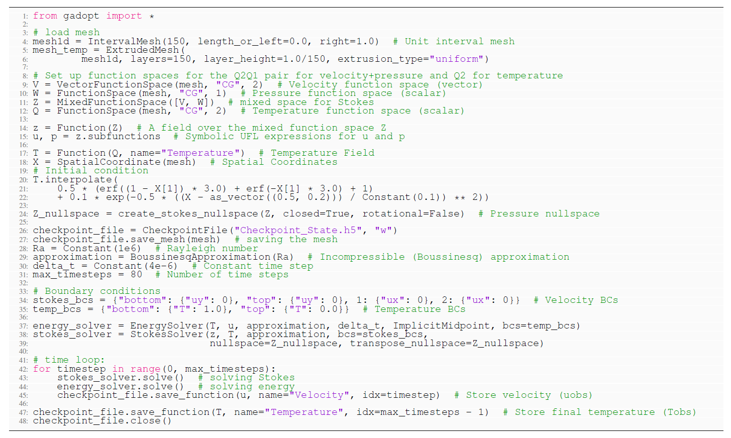
Listing 1 Selected lines from G-ADOPT code, demonstrating generation of our reference isoviscous simulation in an enclosed square domain.

Listing 1 shows selected lines of a G-ADOPT script used to generate this reference synthetic experiment. The first step, illustrated on line 1, is to import the G-ADOPT module (which provides access to Firedrake and associated functionality). We next need a mesh, for which we use a built-in Firedrake meshing function. The computational domain is a unit square with 150×150 elements, loaded on lines 4–6. The function spaces, within which our solutions are defined, are specified as follows:

1. A vector function space, V, is specified for the velocity field (line 9), employing a Q₂ discretisation.

2. A scalar function space, W, is specified for pressure (line 10), utilising a Q₁ discretisation.

3. These are combined on line 11 to create the mixed function space, Z, for the Stokes (velocity and pressure) system.

4. A function space, Q, is specified for the temperature field (line 12), using a Q₂ discretisation.

We specify functions to hold our solutions on lines 14–18. The temperature field, T, is initialised on line 20 using a symbolic expression for the coordinates from line 18. The initialisation includes a 1-D profile along the y axis (line 21) and a Gaussian anomaly, as specified above (line 22). This problem has a constant pressure nullspace, defined as Z_nullspace on line 24, which will subsequently be passed to the solver, and PETSc will seek a solution in the space orthogonal to the provided nullspace. A checkpoint file is initiated on lines 26–27 to retain the necessary fields for the subsequent adjoint inversion. Important constants in this problem (Rayleigh Number, Ra, time-stepping parameters, delta_t and max_timesteps) are defined on lines 28–31, with the Boussinesq approximation specified on line 29 (later passed on to the Stokes and energy systems to determine which terms are to be assembled). Boundary conditions for velocity and temperature are specified on lines 34 and 35, respectively. The latter uses integer mesh markers to tag entities of meshes, with boundaries tagged as follows: tag 1 corresponds to the plane x=0 (left), 2 to x=1 (right), "bottom" to y=0 and "top" to y=1.

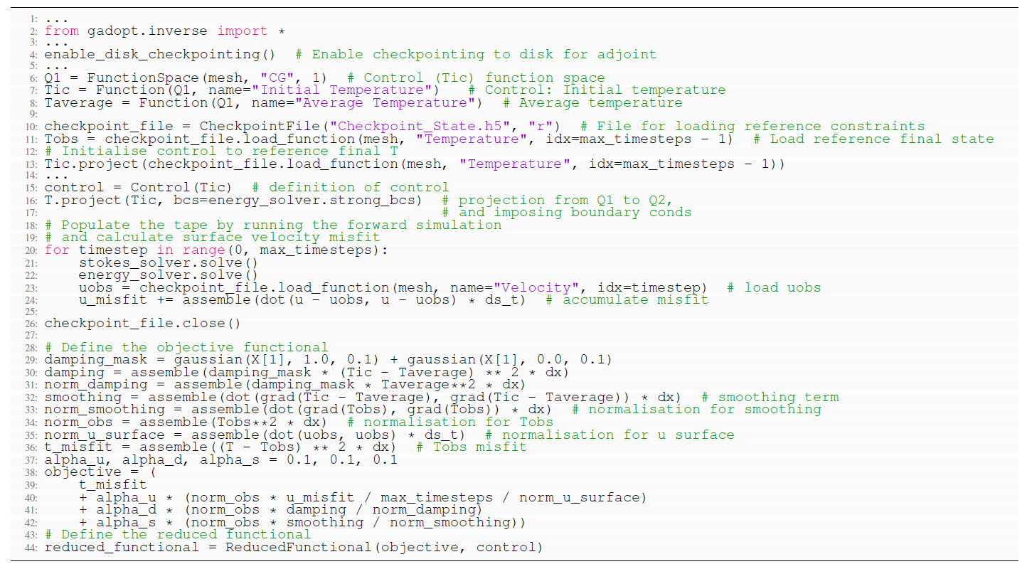
We now solve the variational problem, with solver objects for the energy, energy_solver, and Stokes, stokes_solver, systems created on lines 37 and 38. For the energy system we pass in the solution field T, velocity u, the physical approximation, time step, temporal discretisation approach (i.e. implicit middle point) and boundary conditions. For the Stokes system, we pass in the solution fields z, temperature, the physical approximation, boundary conditions and the nullspace object. The solution of the two variational problems is undertaken by PETSc. The time loop is defined on lines 42–45, with the Stokes system solved on line 43, the energy equation on line 44, and velocities (for later use as time-dependent surface constraints in our adjoint inversions) checkpointed on line 45. Figure 2a to e show temporal snapshots of the reference forward simulation. We note that the final temperature field (Fig. 2e), subsequently utilised in the adjoint inversion, is also checkpointed on line 47.

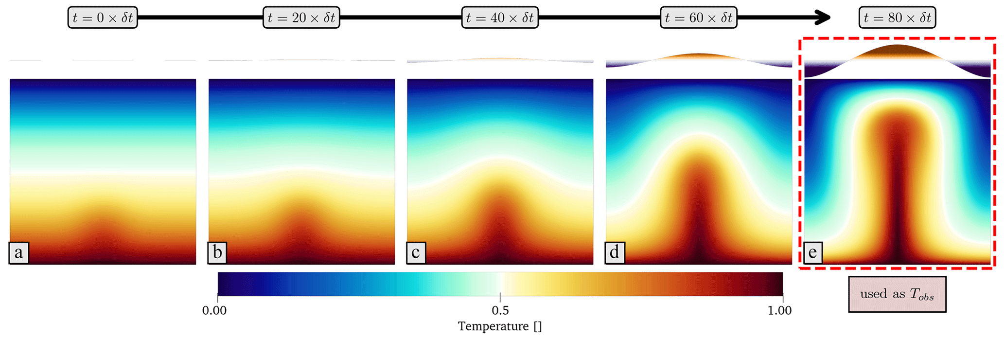
Figure 2 Reference forward simulation: the initial condition is generated by superimposing a Gaussian anomaly of maximum amplitude 0.1 centred at $x_{\mathrm{0}}=(\mathrm{0.5},\mathrm{0.2})$ on top of an adiabatic profile. The simulation runs forward in time from this initial condition, until the plume-like feature approaches the top boundary after 80 time steps. Also visualised at the top of each snapshot are the normal stresses acting on the top boundary, which are proportional to dynamic topography. Boxed in dashed red is the final state of the simulation that is subsequently used as T_obs in our synthetic adjoint simulation.

3.1.2 Inverse problem

Only trivial changes are required to convert the forward problem outlined in Listing 1 into its corresponding adjoint, which are outlined in Listing 2. We first augment our imports with gadopt.inverse (line 2): this provides access to crucial Dolfin-Adjoint functionalities harnessed by Firedrake, enabling overloading differentiation and taping of finite-element operations. On line 4, we activate disc checkpointing of intermediate forward solutions, ensuring that these fields – otherwise retained in memory – are available as inputs for solving the adjoint equations. For this problem, we select the initial temperature as the control, symbolised as Tic on line 7, using a Q₁ function space defined on line 6. On line 8, we define the average temperature field for regularisation terms using the same Q₁ function space. Despite utilising Q₂ elements for the forward temperature computation, opting for a basis function with a lower polynomial degree for the control is advantageous, as it curtails computational expense during the internal optimisation algorithm's operations by reducing the number of degrees of freedom in the solution. Furthermore, using a lower polynomial degree reduces the complexity and regularisation requirements of the optimisation problem, helping to avoid over-fitting of the solution (e.g. Hastie et al., 2009).

On line 10, a checkpoint file is opened. The reference final temperature field is subsequently loaded on line 11, with our guess at the initial temperature condition specified on line 12 (noting that it corresponds to the terminal temperature field of the reference simulation). We specify the control for Dolfin-Adjoint on line 15, followed by projection of the initial temperature condition onto T on line 18. During execution of the time loop (lines 20–24), we solve Stokes and energy systems, after which we load velocities from the reference simulation on line 24, used when accumulating contributions to the surface velocity misfit, u_misfit, on line 24. After the time loop, we define several components of the objective functional. Specifically, we establish the damping term and its associated normalisation factor (lines 29–31), the smoothing term and associated normalisation (lines 32–33), two normalisation terms associated with final state temperature and surface velocity misfits (lines 34–35), and the misfit associated with the final temperature field (line 36). These terms are combined on lines 38–42 as our objective, using weights (α_u, α_d and α_s) specified on line 37, and are later utilised on line 44 to define the reduced functional. We note that values for α_u, α_d and α_s are systematically tested herein.

Listing 2 Changes compared to the forward script in Listing 1 required to define the reduced functional used in the adjoint problem. The three alpha parameters on line 36 denote the three weighting parameters for surface, damping and smoothing terms, respectively.

3.1.3 Investigating the derivative

Our initial guess for T_IC is set to the final “observed” temperature field T_obs (i.e. the terminal temperature field of the forward model). This choice is grounded in the findings of Horbach et al. (2014) and our own tests, which demonstrate that the minimisation problem possesses a strong minimum, rendering it insensitive to the initial guess. The first optimisation iteration starts from this initial guess (Fig. 3a) and runs forward in time to arrive at the first modelled terminal temperature field $T_{t=t_{\mathrm{F}}}$ (Fig. 3b). Compared to the reference T_obs (Fig. 3c), the model is further advanced in time, with the plume tail in the lower mantle narrower and hot buoyant anomalies spread throughout the upper part of the domain, generating a cold return flow and resulting in a thinning of the thermal boundary layers.

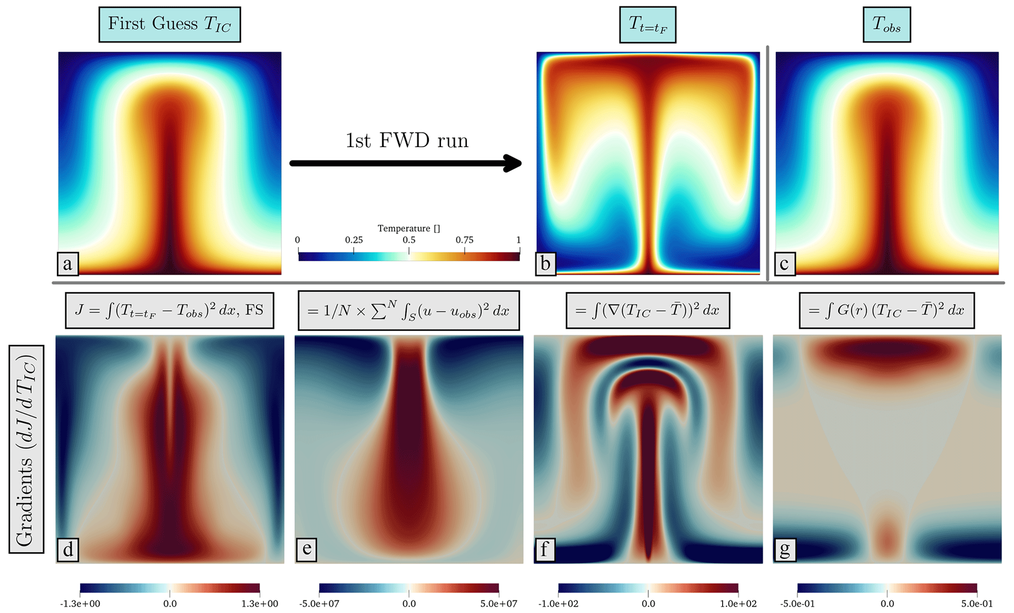
Figure 3 First forward run and associated gradients: (a) is the first guess for T_IC. For all experiments in this study we choose the “observed” temperature field (i.e. the final state) as the initial guess for our optimisations. Panel (b) is the final temperature field after integrating forward in time from (a) for 80 time steps. Panel (c) is the reference final temperature field, T_obs, which is used in the definition of the misfit functional. Panels (d)–(g) illustrate the gradient fields. Panel (e) is gradient of the final temperature misfit. Panel (e) is the gradient of the total surface velocity misfit. Panels (f) and (g) are for the regularising smoothing and damping terms, respectively.

Previously, we noted that for our reconstruction simulations, the objective functional, denoted as J, encompasses four distinct terms: (i) final temperature field, (ii) surface velocity misfit, (iii) smoothing terms and (iv) damping terms. The relevance of the three latter terms is gauged by their respective weighting factors, namely, α_u, α_s and α_d. When combining terms linearly in the objective functional, the superposition principle dictates that the gradient of the entire objective functional is essentially the cumulative sum of the gradients of its constituent terms in J. Consequently, it becomes instructive to visualise and validate the gradient of each individual term within the objective functional.

Figure 3d to g display the gradient fields corresponding to the four terms in the objective functional. The gradient for the final temperature misfit is presented in Fig. 3d: it implies that a better match to the final state temperature field is achievable through changes to the initial condition that include a major reduction in temperature in the domain's centre, complemented by an increase in temperature moving towards the domain's edges, particularly towards the domain's upper regions. In Fig. 3e, we illustrate the gradient of the cumulative surface velocity misfit with respect to T_IC: it reveals sensitivities extending to the domain's base, indicating that to better align with the “observed” surface velocities, an optimal T_IC should be decreased in the middle but increased towards the domain's boundaries. For the smoothing term (Fig. 3f), the highest values emerge in areas with the most abrupt changes in T_IC. Given our optimisation strategy works by moving towards corrections opposite to the gradient's direction, this subsequently results in iterative refinement and smoothing of the solution. For the damping term (Fig. 3g), the gradient aims to minimise fluctuations in the field in relation to the ambient temperature profile ($\overline{T}$), adjacent to the top and bottom boundaries, implying that this can be achieved by reducing boundary layer temperatures in the centre but increasing boundary layer temperatures towards the domain's sides.

3.1.4 Verification of gradients: Taylor remainder convergence test

A fundamental tool used in verification of gradients is the Taylor remainder convergence test (Farrell et al., 2013b). For the reduced functional, J(T_IC), defined in Eq. (6) and its derivative, $\frac{\mathrm{d}J}{\mathrm{d}{T}_{\mathrm{IC}}}$, it can be proven that

$$\begin{array}{}\text{(33)}& \left|J\right(T_{\mathrm{IC}}+h\mathit{\delta }{T}_{\mathrm{IC}})-J(T_{\mathrm{IC}})-h{\displaystyle \frac{\mathrm{d}J}{\mathrm{d}{T}_{\mathrm{IC}}}}\cdot \mathit{\delta }{T}_{\mathrm{IC}}|⟶\mathrm{0}\text{ at }O\left(h^{\mathrm{2}}\right).\end{array}$$

The expression on the left-hand side of Eq. (33) is termed the second-order Taylor remainder. This term's convergence rate of O(h²) serves as a strong foundation for verifying any computational implementation meant for determining $\frac{\mathrm{d}J}{\mathrm{d}{T}_{\mathrm{IC}}}$ (the adjoint code) with respect to a specific functional that computes J(T_IC) (the forward code). Given any arbitrary selection of h and δT_IC, halving the value of h should decrease the magnitude of the second-order Taylor remainder by a factor of 4. Grounded in this theoretical prediction, we employ these so-called Taylor tests to confirm the accuracy of the determined gradients.

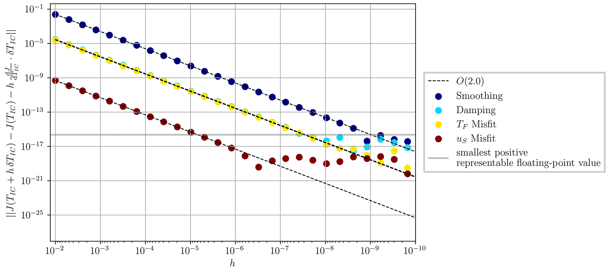
Figure 4 Second-order Taylor remainder test: for each gradient field, the test is performed by computing the functional and the associated gradient when randomly perturbing the initial temperature field T_IC and subsequently dividing the perturbations by a factor of 2 at each level. The dashed line is the theoretical convergence rate of O(2.0). Residuals show accuracy of gradient information down to floating-point precision (defined as the smallest positive ϵ, such that 1.0+ϵ is distinguishable from 1.0.)

We conduct a second-order Taylor remainder test for each term of the objective functional. The results are displayed in Fig. 4, where the gradient fields are calculated for random perturbations of the initial temperature field T_IC, with the amplitude of these perturbations successively halved ($h/\mathrm{2}$, $h/\mathrm{4}$, $h/\mathrm{8}$, ...). Notably, all four Taylor remainder tests demonstrate a convergence rate of O(2.0), extending down to floating-point precision, defined as the smallest positive ϵ such that 1.0+ϵ is distinguishable from 1.0. Our results demonstrate consistency with theoretical expectations, highlighting the robustness of our approach.

3.1.5 Efficiency

Another metric that can be used to assess the suitability of our framework for large-scale mantle convection optimisation problems is the efficiency of derivative calculations. Given the iterative nature of our inverse problem, where derivatives are computed frequently, any efficiency gain, or the lack thereof, can have profound implications for the overall computational cost and feasibility of our automated approach. The computational efficiency can be measured by comparing the computational time of a derivative calculation to that of a forward calculation. Using this reference, a theoretical optimum is defined which measures the ratio of the time that is required to calculate one set of forward and adjoint calculations to one forward calculation. For the Stokes problem we have detailed, in which a linear rheology has been employed, this ratio is considered to be 2.0 (Naumann, 2011; Funke and Farrell, 2013). This is primarily due to the similarity of the forward and adjoint systems. For the simulations presented in this section, we achieve a ratio of 2.01, consistent with theoretical expectations, thus demonstrating the efficiency of our approach.

3.1.6 Optimisation

Executing an optimisation task with G-ADOPT is straightforward. Once the reduced functional is set up (see Listing 2), only a few additional lines of Python are required (see Listing 3). As we use a bounded method for our optimisation problem, we specify a set of upper and lower bounds for the algorithm on lines 3–4. Subsequently, a minimisation problem is outlined (line 6) using both the reduced functional and the designated bounds. This minimisation problem, together with the associated parameters for optimisation, are passed to the Lin–More optimisation algorithm in ROL (line 8), which is executed on line 9.

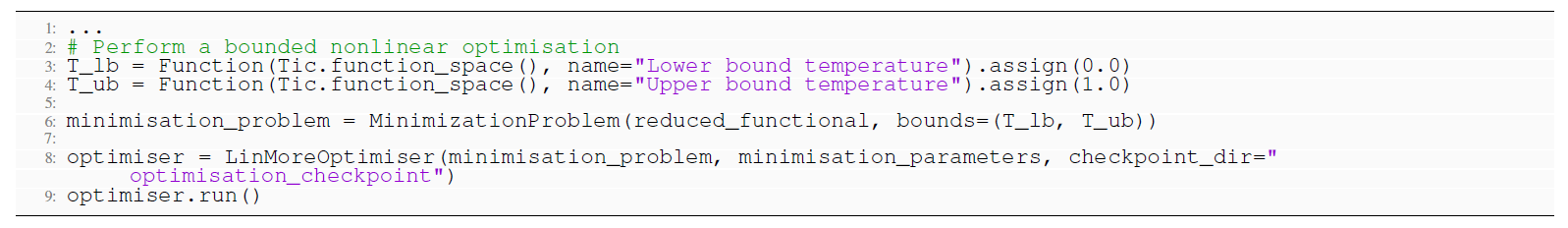
Listing 3 Necessary changes to solve the minimisation problem. T_lb and T_ub are the lower and upper bounds for the minimisation problem, respectively.

Using this framework, we perform a suite of 81 different inverse simulations that aim to find the most optimal combination of the three weightings (α_u, α_d and α_s) that results in the best solution for T_IC when compared to the reference initial temperature field. The simulations are obtained by sweeping through values in ranges of $[{\mathrm{10}}^{-\mathrm{1}},{\mathrm{10}}^{-\mathrm{3}}]$, $[{\mathrm{10}}^{-\mathrm{2}},{\mathrm{10}}^{-\mathrm{4}}]$ and $[{\mathrm{10}}^{\mathrm{1}},{\mathrm{10}}^{-\mathrm{7}}]$ for α_d, α_s and α_u, respectively.

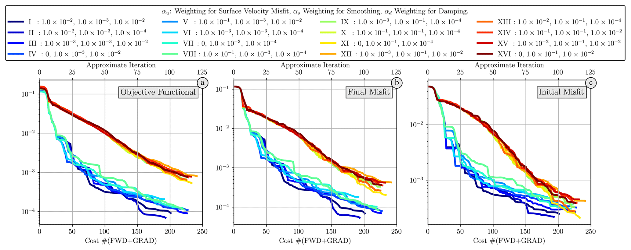
Figure 5 An overview of optimisation results across all experiments: (a) illustrates the minimisation of the objective functional. Panel (b) depicts the final misfit, representing the difference between the reconstructed final temperature field and T_obs. Panel (c) highlights the initial misfit, characterising the discrepancy between the reconstructed initial condition T_IC and the reference initial condition. The bottom horizontal axis in all figures reports the cost, here defined as the sum of forward and derivative calculations. The top axis shows the approximate equivalent number of iterations, which simply is the cost divided by 2. Across all metrics, simulations exhibit a consistent pattern: they converge to the same solution approximately after 100 iterations, though the path to this solution diverges depending on the smoothing weight, α_s.

Figure 5 provides an overview of the outcomes from a subset (16 out of 81) of these optimisation exercises. Minimisation of the objective functional is shown in Fig. 5a, alongside two additional metrics: (i) the misfit between the reconstructed final temperature field and T_obs, termed the final misfit (Fig. 5b), and (ii) the misfit between the reconstructed initial condition, T_IC, and the reference initial condition, highlighting the quality of the reconstructed initial condition (Fig. 5c). The reduction in the metrics in all cases is reported versus the cost, which is the sum of the number of forward and adjoint calculations. A consistent pattern is observed across all reconstruction simulations for these three metrics. Firstly, the solutions are unique, as all converge to a consistent initial condition following roughly 100 iterations (a cost of 200 forward and adjoint calculations). However, the trajectory to this solution varies based on the smoothing weight, denoted by α_s. A significant portion of the simulations with ${\mathit{\alpha }}_{\mathrm{s}}={\mathrm{10}}^{-\mathrm{1}}$ exhibit sub-par performance in the initial stages due to over-smoothing, with most of the best-performing simulations utilising ${\mathit{\alpha }}_{\mathrm{s}}={\mathrm{10}}^{-\mathrm{2}}$. Nevertheless, despite differences in convergence rates, all simulations eventually converge to similar misfits in all three metrics.

Figure 6 showcases multiple iterations from the best-performing simulation using ${\mathit{\alpha }}_{\mathrm{u}}={\mathrm{10}}^{-\mathrm{2}}$, ${\mathit{\alpha }}_{\mathrm{s}}={\mathrm{10}}^{-\mathrm{3}}$ and ${\mathit{\alpha }}_{\mathrm{d}}={\mathrm{10}}^{-\mathrm{2}}$. As mentioned previously, the reference final condition (Fig. 6b) is used as our starting guess for the inverse simulation (Fig. 6c), which yields substantial differences in the modelled final state (Fig. 6k), as illustrated through the squared difference between reconstructed and reference temperature (Fig. 6o). Leveraging derivative information, the inverse simulation corrects the initial condition through an iterative approach. The initial conditions obtained after 20, 50 and 100 iterations are shown in Fig. 6d, e and f, respectively. These solutions reveal that most corrections occur during the initial iterations, with significant improvement in the domain's upper part by iteration 20, albeit with some remaining noise in the solution (see misfit in Fig. 6h). By iteration 100, the solution (visible in Fig. 6f and n) closely mirrors the reference initial condition, represented by misfit values that have diminished by 3 orders of magnitude (Fig. 5b and c).

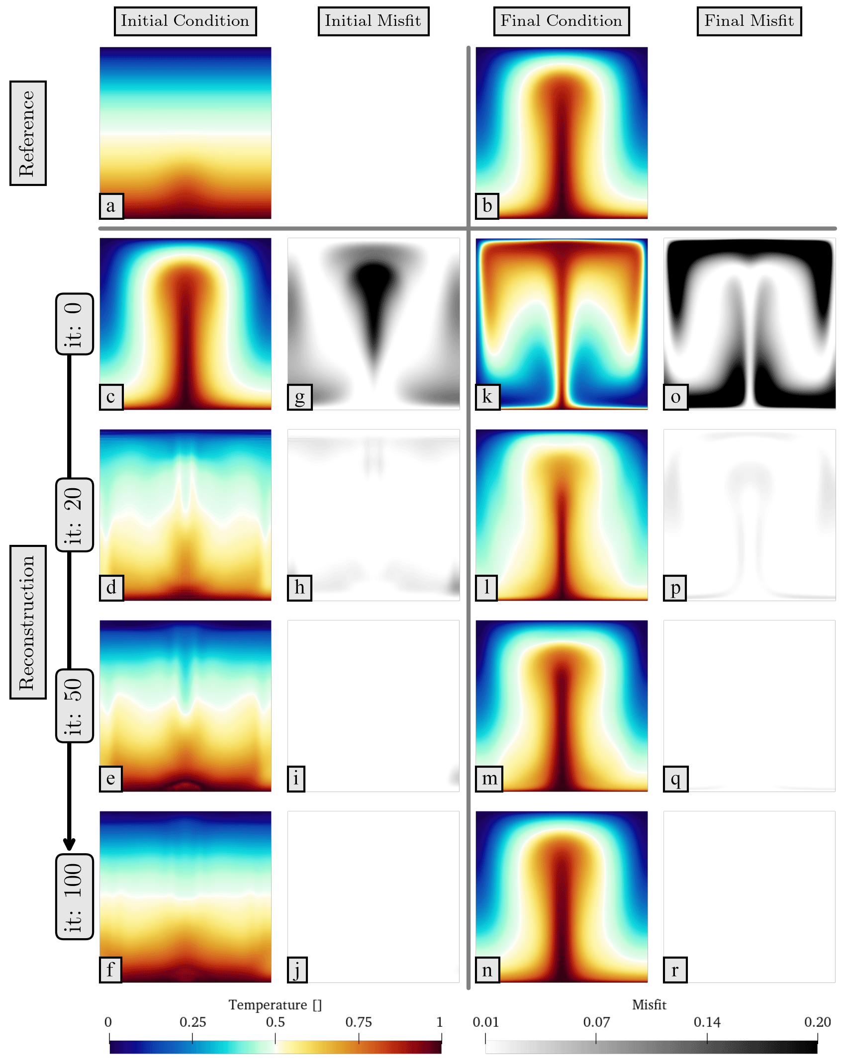
Figure 6 Iterative optimisation process visualised: (a) and (b) depict the reference initial and final conditions. Panels (c)–(f) present the reconstructed initial conditions at the 0th, 20th, 50th and 100th iterations. Panels (g)–(j) highlight the misfits, representing the squared differences between the reconstructed initial temperature fields and the reference temperature. Similarly, (k)–(n) display the reconstructed final temperature fields after the 0th, 20th, 50th and 100th iterations, with their respective misfits demonstrated in (o)–(r).

Figure 7 compares the evolution of reference forward (a–e) and reconstructed simulations (f–j), with differences highlighted (k–o). Furthermore, surface normal stresses are displayed as indicators of surface dynamic topography. For the reconstructed simulation (Fig. 7f), the initial condition is well captured as a Gaussian anomaly in the domain's lower section, superimposed on a depth-dependent field, similar to the reference initial condition. This initial temperature anomaly ascends, culminating at the surface after 80 time steps. The precision of the reconstruction is evident from the misfit panels, with negligible differences between reference and reconstructed simulations throughout the model's evolution (less than 0.01). This is further substantiated by a reduction, by over 4 orders of magnitude, in the objective functional for both initial and end states (Fig. 5b and c). The accuracy of reconstructed surface normal stresses is evidenced by negligible discrepancies in the associated misfit visualisation.

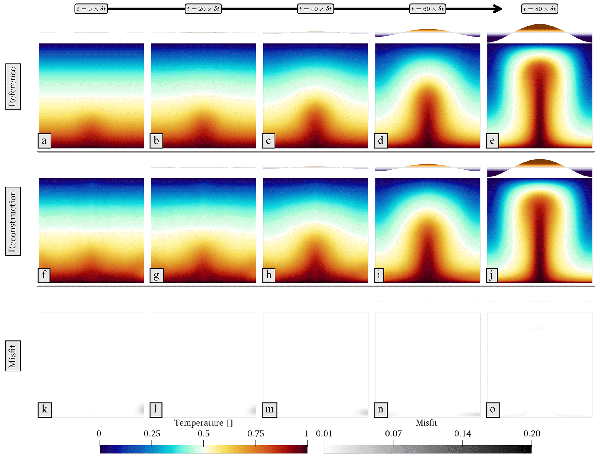
Figure 7 Comparison of reference forward and reconstructed simulations over time: (a)–(e) present the evolution in the reference forward, while (f)–(j) depict the evolution in the reconstructed simulations. The misfits between the reference and reconstructed scenarios at each time step are illustrated in (k)–(o). Note that surface dynamic topography is represented by visualising the normal stresses at the top boundary.

3.2 Convection in an annulus, incorporating a visco-plastic rheology

We next analyse a set of reconstructions which utilise a reference twin that more closely mimics Earth's geometrical and rheological characteristics. We use a 2-D annular domain, generated by extruding 128 times radially from a circular manifold consisting of 512 cells. Inner and outer radii are set to 1.22 and 2.22, respectively, ensuring unit depth and maintaining a comparable ratio between surface and cosmic microwave background (CMB) radii as Earth's mantle. We set Ra=10⁷ and adopt a composite visco-plastic rheology, with effective viscosity determined via a harmonic mean, represented as

$$\begin{array}{}\text{(34)}& \begin{array}{rl}& {\displaystyle \frac{\mathrm{1}}{\mathit{\mu }}}={\displaystyle \frac{\mathrm{1}}{{\mathit{\mu }}_p}}+{\displaystyle \frac{\mathrm{1}}{{\mathit{\mu }}_{\mathrm{lin}}}},\\ & {\mathit{\mu }}_p={\mathit{\mu }}^{*}+{\displaystyle \frac{{\mathit{\sigma }}_{\mathrm{yield}}}{{\mathit{ϵ}}_{ii}}},\\ & {\mathit{\mu }}_{\mathrm{lin}}={\mathit{\mu }}_{\mathrm{0}}\left(r\right)\exp \left({\displaystyle \frac{{\mathrm{\Delta }}_{\mathit{\mu },T}}{T}}\right).\end{array}\end{array}$$

Parameters specified in Eq. (34) are listed in Table 2. As demonstrated by Davies et al. (2022), the changes necessary to transform our forward model from a square to an annular domain and from an isoviscous to a visco-plastic rheology are only minor, noting that Firedrake has already been validated for simulations of this nature (see Davies et al., 2022, and repository accompanying this paper for a comprehensive script).

To determine the reference simulation's initial condition, we commence from a starting state with small-scale spherical harmonic perturbations and advance forward in time until a quasi-steady state is achieved (i.e. when basal and surface heat fluxes are roughly in balance). The resulting state (Fig. 8.1.A and 2.A), which contains downwellings that descend from the upper thermal boundary layer and upwelling plumes that rise from the lower thermal boundary layer, forms our reference initial condition. We subsequently advance forward for a duration of $t=\mathrm{200}\times (\mathrm{5}\times {\mathrm{10}}^{-\mathrm{6}})$ to reach the reference final state shown in Fig. 8.1.G. While the non-dimensional time of 10⁻³ translates into 256 Myr of convection, the domain velocities suggest an equivalent Earth-like time of ≈ 100 Myr (due to a marginally reduced Ra relative to estimates for Earth's mantle). The sequence presented in Fig. 8.1.A–G and 2.A–G trace the temporal development of reference temperature and viscosity fields, respectively. The viscosity field spans approximately 3 orders of magnitude, extending from low asthenospheric values of ≈1.0, rising to 140 within the cooler segments of the lower mantle, and decreasing to 0.4 in locations of high strain rates at surface convergent boundaries.

Table 2 Parameters employed for 2-D annulus twin experiments.

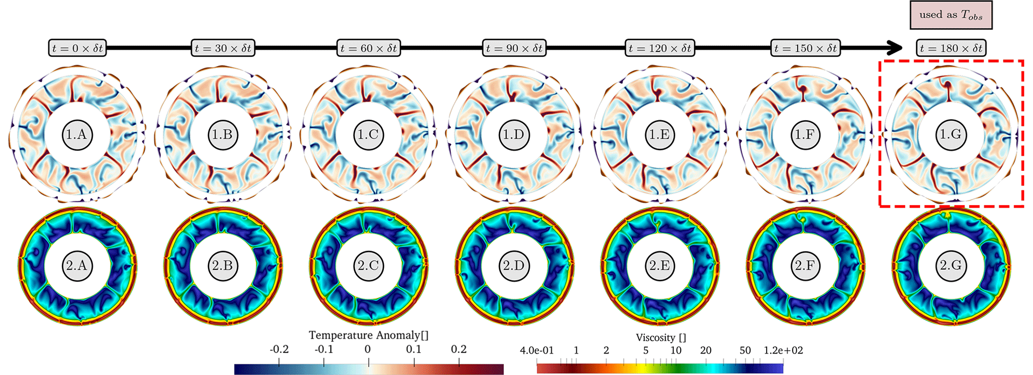
Figure 8 Reference forward simulation spanning a duration of $t=\mathrm{200}\times (\mathrm{5}\times {\mathrm{10}}^{-\mathrm{6}})$, as depicted in (1.A) to (1.G). Panels (1) (upper row) detail the temporal evolution of the reference temperature field, while Panels (2) (lower row) show the viscosity field at each time. The viscosity demonstrates a variation of nearly 3 orders of magnitude: approximately 1.0 in the asthenosphere, 140 within colder lower-mantle slabs and 0.4 in convergent regions exhibiting elevated strain rates.

3.2.1 Verification of gradients

As with the previous Cartesian case examined, reconstruction simulations are conducted with an objective functional encompassing the misfit component related to the terminal temperature field, accumulative surface velocity misfits and regularisation terms. For consistency with the previous case, we first confirm the accuracy of the calculated gradient fields corresponding to each component in the objective functional by performing second-order Taylor remainder convergence tests. To further analyse the robustness of our results against solver tolerances, specifically concerning the final temperature field and surface velocities, we conduct a set of two additional convergence tests. The first set utilises a Newton (SNES) relative solver tolerance of 10⁻¹⁰ and is depicted using solid colours in Fig. 9, while the second set, using a relative tolerance of 10⁻⁵, is represented by semi-transparent colours. Our findings indicate that with tighter tolerances, results adhere to an O⁻² trend consistent with theoretical predictions, confirming accuracy down to the smallest floating-point representation. Conversely, when the tolerance is relaxed to 10⁻⁵, this behaviour holds only up to perturbations of similar magnitude ($h\approx {\mathrm{10}}^{-\mathrm{5}}$), demonstrating a divergence from the expected O(h²) trend for smaller perturbations.

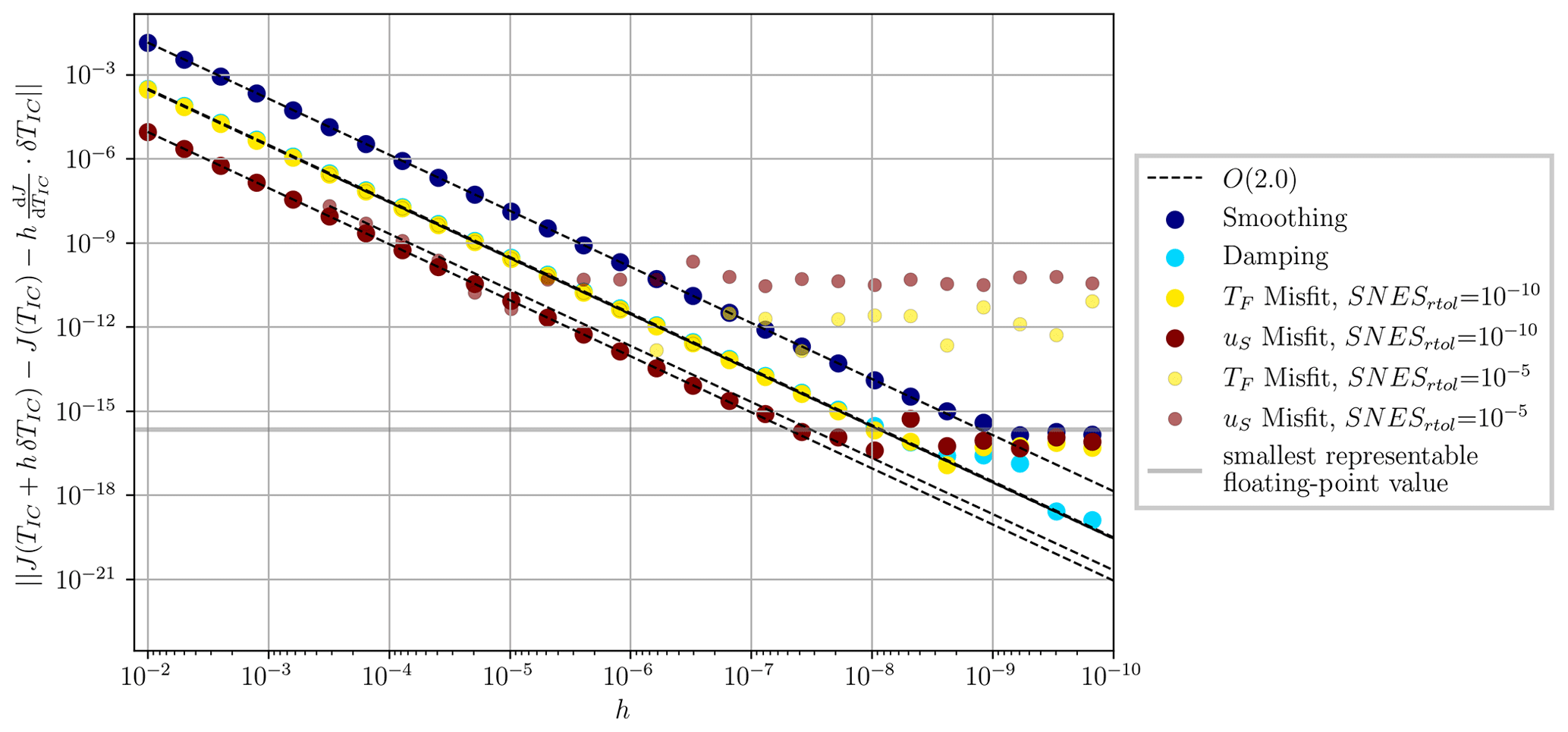
Figure 9 Second-order Taylor remainder test for convection with a temperature-, depth- and stress-dependent rheology. The semi-transparent markers are cases where the relative solver tolerance of Newton solves (SNES) is set to 10⁻⁵. With such tolerances, perturbations beyond solver tolerance exhibit divergence from the O(h²) trend. When setting this tolerance to 10⁻¹⁰ (larger solid markers), residuals show accuracy of gradient information down to floating-point precision.

3.2.2 Efficiency

In the experiments detailed in this section, an efficiency of 1.45 is achieved. This exceeds the previously outlined theoretical efficiency of 2.0 for the isoviscous Stokes model in Sect. 3.1.5 due to a major difference in the forward and adjoint momentum equations: while the forward momentum equation employs a non-linear visco-plastic rheology and requires multiple linear Newton solves per time step, the adjoint momentum remains linear. The forward model is therefore more computationally demanding, explaining the improved efficiency ratio.

3.2.3 Optimisation

As highlighted with our previous example, absolute and relative variations in weighting of different objective functional components can generate solutions with distinct properties, some of which provide an improved match to the reference simulation. Accordingly, it is vital to assess the consequences of these distinct weight combinations for the case considered here. To address this, we have undertaken 21 simulations, adjusting the parameters α_u, α_s and α_d within the intervals [0.05,0.1], [0.01,0.1] and [0.01,0.1], respectively, with values motivated by the results of our previous set of simulations. The collective convergence of all 21 simulations is illustrated in Fig. 10.

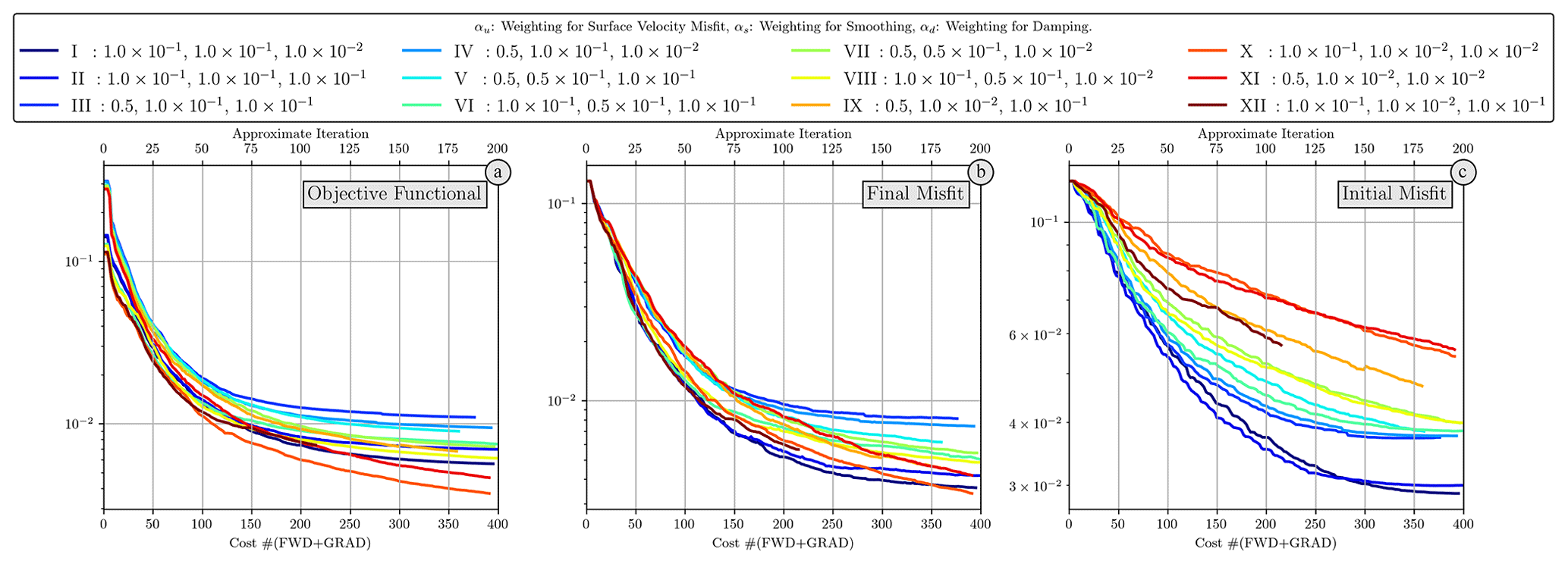
Figure 10 Summary of optimisation outcomes from 2-D annulus experiments. Panel (a) visualises the process of objective functional minimisation. Panel (b) illustrates the final misfit, representing the misfit between the reconstructed final temperature field and T_obs. Panel (c) depicts the initial misfit, indicating the difference between the reconstructed initial condition T_IC and the reference initial condition. Notably, despite significant reduction in the objective functional and final misfit in simulations XI and XII, these simulations do not perform as well in terms of the initial misfit, which is a key measure in our experiments.

Our objective functional (Fig. 10a) has initial values that range between $\sim \mathrm{1}\times {\mathrm{10}}^{-\mathrm{1}}$ and $\mathrm{2}\times {\mathrm{10}}^{-\mathrm{1}}$. We consistently observe a reduction of an order of magnitude or more in this measure. Notably, the steepest decline is seen within the initial 50 iterations (cost ∼100). The simulations denoted as X and XI exhibit the largest reduction, with a consistent reduction trajectory even when approaching iteration 200 (cost ∼400).

The final temperature misfit (Fig. 10b) exhibits different trends to the objective functional. In the initial iterations, the largest reductions in final misfit are observed for simulations I and II, with simulation XII trailing behind. Despite displaying a lower misfit reduction up until iterations 140 and 180 (cost ∼280–360), simulations X and XI eventually display a similar misfit by iteration 200 (cost ∼400). When we turn to reduction in the initial misfit (Fig. 10c), an entirely different trend comes to light: simulations I and II sustain their reduction until around iteration 150 (cost ∼300), after which they plateau. Conversely, many other simulations plateau at misfit values that are, on average, twice as high.

In our analysis, the reconstruction quality is predominantly governed by three key weighting parameters: surface velocity misfit (α_u), smoothing (α_s) and damping (α_d). These parameters calibrate the significance of different objective terms in relation to the final temperature misfit term. Thus, the primary metric to assess a reconstruction is the simultaneous reduction in misfits for both initial and final states. Incorporating the misfit associated with surface velocities enhances the quality of the reconstructions, noting that higher weightings of the surface velocities require higher values of smoothing. Among the weighting parameters, α_s is shown to have the highest effect in convergence outcomes: higher values for α_s lead to over-regularisation, thereby limiting the role of sensitivity information tied to misfit terms in the solution. α_d offers a more varied range of effective values, which aligns with its role confined to thermal boundary layers and, consequently, its lesser impact on the overall numerical domain. Therefore, Case I, characterised by $({\mathit{\alpha }}_{\mathrm{u}},{\mathit{\alpha }}_{\mathrm{s}},{\mathit{\alpha }}_{\mathrm{d}})=(\mathrm{1}\times {\mathrm{10}}^{-\mathrm{1}},\mathrm{1}\times {\mathrm{10}}^{-\mathrm{1}},\mathrm{1}\times {\mathrm{10}}^{-\mathrm{2}})$, emerges as the optimal set of weighting parameters for our reconstructions.

In contrast to the reduction of 3 orders of magnitude in the misfit functions from the isoviscous experiment, our non-linear experiment exhibits a modest reduction of O(1). The key factor contributing to this is the extended total simulation time for the non-linear experiment. Representing a far longer reconstruction period, this implies more information loss during the inversion process. Additionally, while the isoviscous experiment focused on a single temperature anomaly, this simulation tackles whole-mantle convection, with numerous and occasionally complex and highly time-dependent anomalies, reflecting the more intricate visco-plastic rheology. Nonetheless, this reduction of an order of magnitude in misfit translates into a satisfactory reconstruction of the initial condition, demonstrating the efficacy and robustness of the numerical approaches employed.

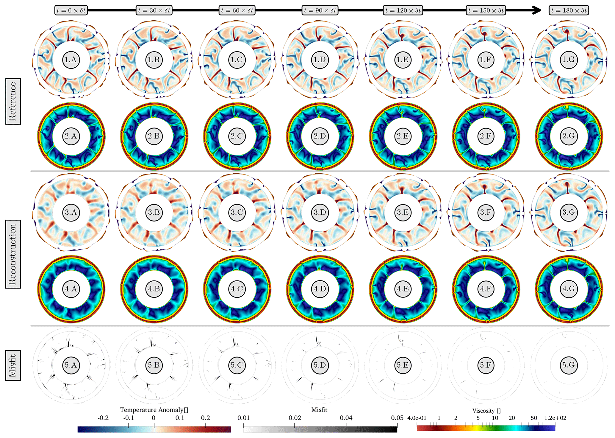
Figure 11 Comparing the reference (1, 2) and the best reconstruction simulation (3, 4). Temperature and viscosity fields are shown in panels (1, 3) and (2, 4), respectively. The misfit, which is the squared difference between the reconstructed and reference temperatures, is shown in panel (5). To highlight the effectiveness of the reconstruction of the evolution of surface dynamic topography, a field representing the normal stresses acting on the top boundary is visualised alongside the temperature fields in (1) and (3). The reconstruction simulation employs values of ${\mathit{\alpha }}_{\mathrm{u}}={\mathrm{10}}^{-\mathrm{1}}$, ${\mathit{\alpha }}_{\mathrm{s}}={\mathrm{10}}^{-\mathrm{1}}$ and ${\mathit{\alpha }}_{\mathrm{d}}={\mathrm{10}}^{-\mathrm{2}}$ and is marked with I in Fig. 10.

This is confirmed by visual inspection of the best reconstruction model, with temperature, viscosity and surface normal stresses presented and compared to the reference case in Fig. 11 (marked case I in Fig. 10, using values of ${\mathit{\alpha }}_{\mathrm{u}}={\mathrm{10}}^{-\mathrm{1}}$, ${\mathit{\alpha }}_{\mathrm{s}}={\mathrm{10}}^{-\mathrm{1}}$ and ${\mathit{\alpha }}_{\mathrm{d}}={\mathrm{10}}^{-\mathrm{2}}$). At t=0, the reconstructed temperature field exhibits upwelling and downwelling features that are reconstructed in the correct locations, although temperature anomalies are generally smoother than those of the reference case (Fig. 11.1.A). The corresponding viscosity field mirrors this smoothness despite capturing weaker convergence zones at the surface. Despite these variations, the spatial misfit is generally below 10⁻² (Fig. 11.5.A) with errors over 0.05 restricted to sharper features that are inevitably smoothed in the reconstruction process. This smoothness is also reflected in recovered surface normal stresses, with highs and lows correctly positioned, albeit at longer wavelengths than the reference case.

Given the application of a free-slip boundary condition at the surface of this simulation, a prominent outcome of this set of experiments is the emergence of sharp subducting slabs and weak zones at the top boundary as the simulation evolves (Fig. 11.3.B and 4.B). The marked decrease in misfit over time (Fig. 11.5.B) confirms the development of more detailed convective patterns. As the simulation evolves, reconstructed plume features become more precise, and reconstructed surface normal stresses more closely resemble the reference case. This enhancement progresses up to the final time step, where the reconstructed thermal field and surface normal stresses are indistinguishable from those in the reference simulation, reflected via an order of magnitude reduction in the spatial misfit field.

4 Discussion

Robust reconstructions of the spatial and temporal evolution of Earth's mantle and its diverse surface expressions are critical to scientific progress across the geosciences. It requires the construction of a digital twin: a vital instrument for analysing and revealing the complex interplay between the mantle and Earth's other systems. To this end, the adjoint method provides the necessary means for obtaining and analysing model sensitivities with respect to earlier mantle states. A burgeoning number of studies exploiting this methodology for reconstructions of mantle convection have emerged in recent years (e.g. Bunge et al., 2003; Ismail-Zadeh et al., 2004; Liu et al., 2010; Spasojevic et al., 2009; Li et al., 2017; Price and Davies, 2018; Ghelichkhan et al., 2021). Nevertheless, the derivation, implementation and validation of adjoint systems for coupled, non-linear, time-dependent systems remain notoriously difficult. It is due to these difficulties that existing applications of the geodynamic adjoint method often include major simplifications, either incorporating an oversimplified treatment of mantle rheology (e.g. Colli et al., 2018; Ghelichkhan et al., 2021), neglecting certain (coupling) terms in the adjoint equations (e.g. Ismail-Zadeh et al., 2004) or both (e.g. Liu and Gurnis, 2010): they are therefore likely limited in their applicability to realistic Earth scenarios. In this study, we leverage the latest advances in scientific computing to overcome these limitations and develop G-ADOPT, an open-source numerical framework for geoscientific adjoint reconstructions, developed in full compliance with FAIR (Findable, Accessible, Interoperable, Reusable) principles (Wilkinson et al., 2016).

G-ADOPT is underpinned by three primary software elements. The first is Firedrake (Ham et al., 2023), an automated system for solving partial differential equations using the finite-element method. In our previous work (Davies et al., 2022) we examined the applicability of Firedrake to geodynamical simulations, confirming its accuracy, efficiency, extensibility and parallel scalability through comprehensive benchmarks and state-of-the-art mantle convection simulations. The second element is Dolfin-Adjoint (Farrell et al., 2013a; Mitusch et al., 2019), a system that automatically generates the discrete adjoint from forward models designed in Firedrake. Dolfin-Adjoint elevates the conventional abstraction of automatic differentiation from individual floating-point operations to complete systems of differential equations, leveraging the high-level mathematical abstraction of finite-element problems and their symbolic representation in UFL (Alnæs et al., 2014). The adjoint systems derived by Dolfin-Adjoint are UFL expressions and valid Firedrake inputs. Therefore, they inherit the parallel support native to the forward model, which results in optimal computational efficiency. The third element is the Rapid Optimisation Library, ROL, a Trilinos package for large-scale optimisation problems (The ROL Project Team, 2022), enhanced herein with intra-optimisation checkpointing functionality.

We have demonstrated the applicability of G-ADOPT for time-dependent geodynamic reconstructions herein. The objective functional utilised in our reconstructions is composed of two distinct misfit components. The first is a term that quantifies the misfit corresponding to the observed final state temperature field, analogous to the present-day temperature field within Earth's mantle as obtained through a combination of mantle mineralogical models (e.g. Stixrude and Lithgow-Bertelloni, 2011; Chust et al., 2017) and seismic imaging (e.g. Rawlinson et al., 2010; French and Romanowicz, 2014; Simmons et al., 2015; Bozdağ et al., 2016; Koelemeijer et al., 2016; Fichtner et al., 2018). The second term corresponds to observed surface velocities, accessible through plate tectonic reconstruction models (e.g. Müller et al., 2019). Additionally, smoothing and damping terms have been incorporated to enforce regularity in our solutions.

Our study analysed two sets of reconstructions of systematically increasing complexity. We first examined the evolution of a single ascending hot anomaly in an enclosed isoviscous square domain. By taking advantage of the simplicity of the geometry and rheological properties, we were able to deliver an in-depth examination of the gradients for each term, including a parameter-space search to ascertain optimal weighting parameters. Our results reveal a general convergence of the solutions, notwithstanding substantial variations in convergence rates subject to the weightings. Additionally, although not detailed in this paper, we have explored a number of different optimisation methods and parameters. Through this comprehensive analysis, we are confident that the problem possesses a stable solution that can be found through an appropriate combination of weighting parameters. The second set of reconstruction experiments explored convection with a stress-, depth- and temperature-dependent rheology at the convective vigour of Earth's mantle, demonstrating the feasibility of reconstruction studies for Earth's mantle with a non-linear rheology. The weightings selected for this series of experiments were broadly consistent with the first set. Given the success at reproducing surface velocities and normal stresses, our findings suggest that reconstruction models of Earth's mantle can serve as a powerful means for probing changes in the landscape at Earth's surface induced by mantle dynamics (e.g. Friedrich et al., 2018; Hoggard et al., 2021; Davies et al., 2023).

In both experimental sets, we assessed the numerical efficiency of our framework by evaluating the cost ratio between forward and adjoint calculations. In the first set, our results produced a ratio of 2.01, aligning with the theoretical efficiency of 2.0 (e.g. Naumann, 2011). In the second set, where we solved the non-linear forward equations, we observed a ratio of 1.45. This efficiency is attributed to the linearised nature of the adjoint method: even when applying non-linear rheologies in the forward equations, the adjoint equations remain linear. We also conducted second-order Taylor remainder convergence tests for each of the objective functional terms to validate the adjoint calculations. We note our convergence is accurate down to floating-point precision, consistent with results presented by Coltice et al. (2023). Our assessments demonstrate the accuracy of the derivative calculations (Figs. 4 and 9). These Taylor remainder convergence tests provide a robust basis for future validations of geodynamic adjoint frameworks.

Our experiments incorporate two significant simplifications relative to realistic-Earth scenarios, which were necessary to facilitate the number of reconstruction simulations analysed: (i) the use of a 2-D computational domain and (ii) the application of the Boussinesq approximation instead of more pertinent approximations such as anelastic-liquid approximations (e.g. Jarvis and McKenzie, 1980). Nevertheless, the composable nature of G-ADOPT should alleviate any concerns regarding the extensibility of our framework to these more realistic problem sets. Our prior work in Davies et al. (2022) demonstrates the flexible nature of our approach: for example, transitioning our 2-D annulus simulations to a 3-D spherical shell domain can be achieved via changes to only a few lines of Python. The application of G-ADOPT for reconstructing Earth's mantle evolution using non-linear rheologies and compressibility will be the subject of future investigations, although we note that the forward modelling approach has already been developed (Davies et al., 2022). Moreover, our framework is extendable to various other problems in geodynamics. These include utilising principal stress directions (e.g. Reuber et al., 2020), surface plate velocities (e.g. Ratnaswamy et al., 2015; Bocher et al., 2018) and/or residual depth measurements (e.g. Panasyuk and Hager, 2000; Spasojevic et al., 2009) to explore the mantle's rheological properties and to study the visco-elastic adjustment of Earth's surface in response to the melting of Earth's polar ice sheets (Al-Attar and Tromp, 2014; Martinec et al., 2015, e.g.) and post-seismic deformation following significant subduction earthquakes (e.g. Sabadini and Vermeersen, 1997).

Reconstructing past mantle states is fraught with substantial theoretical and practical challenges. In this study, we targeted some of these theoretical and practical hurdles by introducing G-ADOPT. Nevertheless, significant obstacles exist that are beyond the scope of this work. We predicated our work on zero uncertainty in our reference fields (i.e. the present-day temperature field and past surface velocities), thereby committing what is known as the “inverse crime” (Colton et al., 1998), a term used to describe the situation when the code employed in the inversions is also utilised to generate reference simulations. Estimation of the present-day mantle state from seismic imaging and the assumptions regarding the thermal and compositional interpretation of seismic heterogeneity are both fraught with considerable uncertainty (e.g. Styles et al., 2011; Mosca et al., 2012; Zaroli et al., 2013; Davies et al., 2015). Furthermore, plate tectonic reconstructions can be uncertain, particularly further back in time and within the Pacific region (e.g. Shephard et al., 2012; Williams et al., 2015; Tetley et al., 2019). However, the existence of seafloor spreading isochrons up to approximately 125 Ma for all major plates provides confidence in modelling relative plate movements in more recent geological periods (Seton et al., 2020). An uncertainty impact study carried out by Colli et al. (2020) posits that the presence of uncertainties causes reconstructed and reference flow histories to diverge exponentially back in time, with unrealistic structures materialising within and adjacent to thermal boundary layers. To minimise these impacts, Colli et al. (2020) advocate for terminating the optimisation after a few iterations. Here, however, the inclusion of regularisation terms in the objective functional mitigates these impacts, effectively constraining the reconstruction to a smoother solution. This becomes particularly advantageous in real-Earth applications where observational constraints become sparser and more uncertain back in time. Without a smoothing term, the solution to the initial condition can contain high-frequency noise, which would diffuse over the course of the simulation. Smoothing therefore drives the solution towards a longer-wavelength initial state whilst maintaining sensitivity to shorter wavelength information recorded in seismic tomography images.

Moreover, by formally introducing past surface velocities into the objective functional, we infuse sensitivity information that propagates further back in time, refining the flow trajectory to improve the accuracy of reconstructions in the upper thermal boundary layer region. This sets our approach apart from the method used in previous adjoint reconstruction simulations (e.g. Vynnytska and Bunge, 2015; Zhou and Liu, 2017; Ghelichkhan et al., 2021), where the sequential-in-time nature of plate velocity assimilation can improve flow trajectories only forward in time. Despite this, it is crucial to recognise that observed surface velocities are the result of a complex force balance, including contributions from within Earth's mantle and at Earth's surface, including those at plate boundaries, such as the genesis and destruction of orogenies, which have been associated with rapid changes in plate velocities (Colli et al., 2014; Iaffaldano and Bunge, 2015). These forces are not captured in current state-of-the-art spherical mantle convection models. Although our inversions utilise absolute plate velocities – thereby accounting for the majority of the forces driving surface movements – it is essential to emphasise that constraints on Earth's present-day thermal field must be prioritised as the primary data source for such inversions.

Our study lays the foundations for exploring several unresolved geodynamical questions. Previous research has shown that prescribing plate tectonic reconstruction velocities as a top boundary condition improves the precision of mantle reconstruction models and diminishes noise (e.g. Colli et al., 2015; Taiwo et al., 2023). Our framework formally incorporates these constraints through misfit terms, and future studies should compare this with other methods to find the most efficient way to integrate these valuable data. Earlier research advocates solving the reduced adjoint system, effectively considering velocities as insensitive to initial conditions (e.g. Ismail-Zadeh et al., 2004; Liu et al., 2008). The second-order Taylor remainder convergence tests, examined herein, provides a robust foundation for evaluating the accuracy of such simplifications. Furthermore, our framework sets the stage for including hitherto unused observations within our inversions, such as geochemical constraints on mantle temperature and pressure (Ball et al., 2021). This stems from the design principle of composable abstractions in the software packages used in G-ADOPT, ensuring all components' modularity, interoperability, reusability, scalability and maintainability. Specifically, Firedrake emphasises a clear separation between using the finite-element method and implementing it. Dolfin-Adjoint automates the derivation and computation of the adjoint systems using high-level symbolic language, ensuring the same advanced strategies that are applied for the forward calculation are utilised in the adjoints. Finally, ROL offers large-scale optimisation algorithms that seamlessly integrate with Firedrake and Dolfin-Adjoint. Their integration through G-ADOPT is a ground-breaking development that opens up adjoint problems to a new class of user and developer.

5 Conclusions

Transitioning from idealised forward models to data-driven simulations necessitates an inverse approach that rigorously incorporates observational constraints and their uncertainties. The adjoint method has emerged as a key technique for optimising unknown model parameters against observational data (e.g. Bunge et al., 2003). In this context, we introduce the Geoscientific ADjoint Optimisation PlaTform (G-ADOPT), which capitalises on cutting-edge developments in computational sciences, particularly through innovations in Firedrake (e.g. Rathgeber et al., 2016; Davies et al., 2022), Dolfin-Adjoint (Farrell et al., 2013a; Mitusch et al., 2019) and the Rapid Optimisation Library (ROL) (The ROL Project Team, 2022).

Our investigation, validated by two distinct sets of twin experiments, demonstrates G-ADOPT's efficacy in deducing the initial conditions for mantle flow and tracing its progression through space and time. These synthetic experiments leverage misfit terms to integrate both contemporary constraints across the computational domain and temporal constraints at Earth's surface. Additionally, we explored regularisation techniques to modulate the amplitude and complexity within the optimal solution. Notwithstanding the simplifications made (e.g. neglecting compressibility and 3-D geometry), G-ADOPT's architecture allows for straightforward adaptation to more complex scenarios with minimal modifications to the Firedrake forward model (as evidenced by Davies et al., 2022), alongside automated adjoint derivation and computation via Dolfin-Adjoint. The employment of the second-order Taylor remainder convergence test further corroborates our methodology, establishing a precedent for the advancement of geodynamic adjoint frameworks and facilitating prompt validation of adjoint models for more complex analyses.

Historically, geoscientific modelling frameworks were tailored to specific equations, which limited their application across disciplines. The current progress in adjoint-based techniques, crucial for data assimilation, sensitivity analysis and optimisation, has markedly benefited meteorology and oceanography, though similar progress in other fields has been hindered by derivation and implementation challenges. G-ADOPT's modular design seeks to bridge these divides. Its components are designed for ease of assembly and reusability, promoting a culture of modular, interoperable, scalable and maintainable methods and frameworks. This philosophy ensures that G-ADOPT can be readily adapted to a broad spectrum of geoscientific research areas.