Development and evaluation of the interactive Model for Air Pollution and Land Ecosystems (iMAPLE) version 1.0

Land ecosystems are important sources and sinks of atmospheric components. In turn, air pollutants affect the exchange rates of carbon and water fluxes between ecosystems and the atmosphere. However, these biogeochemical processes are usually not well presented in Earth system models, limiting the explorations of interactions between land ecosystems and air pollutants from regional to global scales. Here, we develop and validate the interactive Model for Air Pollution and Land Ecosystems (iMAPLE) by upgrading the Yale Interactive Terrestrial Biosphere Model with process-based water cycles, fire emissions, wetland methane (CH₄) emissions, and trait-based ozone (O₃) damage. Within iMAPLE, soil moisture and temperature are dynamically calculated based on the water and energy balance in soil layers. Fire emissions are dependent on dryness, lightning, population, and fuel load. Wetland CH₄ is produced but consumed through oxidation, ebullition, diffusion, and plant-mediated transport. The trait-based scheme unifies O₃ sensitivity of different plant functional types (PFTs) with the leaf mass per area. Validations show correlation coefficients (R) of 0.59–0.86 for gross primary productivity (GPP) and 0.57–0.84 for evapotranspiration (ET) across the six PFTs at 201 flux tower sites and yield an average R of 0.68 for CH₄ emissions at 44 sites. Simulated soil moisture and temperature match reanalysis data with high R above 0.86 and low normalized mean biases (NMBs) within 7 %, leading to reasonable simulations of global GPP (R=0.92, NMB=1.3 %) and ET (R=0.93, $\text{NMB}=-\mathrm{10.4}$ %) against satellite-based observations for 2001–2013. The model predicts an annual global area burned of 507.1 Mha, close to the observations of 475.4 Mha with a spatial R of 0.66 for 1997–2016. The wetland CH₄ emissions are estimated to be 153.45 Tg [CH₄] yr⁻¹ during 2000–2014, close to the multi-model mean of 148 Tg [CH₄] yr⁻¹. The model also shows reasonable responses of GPP and ET to the changes in diffuse radiation and yields mean O₃ damage of 2.9 % to global GPP. iMAPLE provides an advanced tool for studying the interactions between land ecosystems and air pollutants.

1 Introduction

As an important component on the Earth, land ecosystems regulate global carbon and water cycles. Every year, the terrestrial ecosystem assimilates ∼120 Pg (1 Pg=10¹⁵ g) of carbon from the atmosphere through vegetation photosynthesis (Beer et al., 2010). However, most of this carbon uptake returns to the atmosphere due to plant and soil respiration (Sitch et al., 2015), as well as other perturbations such as biomass burning and biogenic emissions (van der Werf et al., 2010; Carslaw et al., 2010), leading to a net carbon sink of only ∼2 Pg C yr⁻¹ during 1960–2021 (Friedlingstein et al., 2022). Meanwhile, land ecosystems affect atmospheric moisture and soil wetness through both physical (e.g., evaporation and runoff) and physiological (e.g., leaf transpiration and root hydrological uptake) processes. Observations show that transpiration accounts for 80 %–90 % of the terrestrial evapotranspiration (ET) (Jasechko et al., 2013) and makes significant contributions to land precipitation, especially over the tropical forests (Spracklen et al., 2012).

Different approaches have been applied to depict the spatiotemporal variations of ecosystem processes. The eddy covariance technique provides direct measurements of land carbon and water fluxes (Jung et al., 2011). However, the limited number and uneven distribution of ground sites result in large uncertainties in the upscaling of site-level fluxes to the global scale (Jung et al., 2020). Satellite retrieval provides a unique tool for the continuous representation of land fluxes in both space and time (Worden et al., 2021). However, most of the ecosystem variables (e.g., gross primary productivity, GPP) can only be derived using available signals from remote sensing through empirical relationships (Madani et al., 2017). As a comparison, process-based models build physical parameterizations based on field and/or laboratory experiments and validate against the available in situ and satellite-based observations (Niu et al., 2011; Castillo et al., 2012). These models can be further applied at different spatial (from site to global) and temporal (from days to centuries) scales to identify the main drivers of the changes in carbon and water fluxes (Sitch et al., 2015). For example, a total of 17 vegetation models were validated and combined to predict the land carbon fluxes in the past century (Friedlingstein et al., 2022); the ensemble mean of these models revealed a steadily increasing land carbon sink from 1960 with the dominant contribution by CO₂ fertilization.

While many studies have quantified the ecosystem responses to the effects of CO₂, climate, and human activities (Piao et al., 2009; Sitch et al., 2015), few have explored the interactions between air pollution and land ecosystems. Such biogeochemical processes are becoming increasingly important in the Anthropocene period with significant changes in atmospheric compositions. For example, observations found that nitrogen and phosphorus constrain the CO₂ fertilization efficiency of global vegetation (Terrer et al., 2019), but such a limiting effect is ignored or underestimated in most of the current models (Wang et al., 2020). Tropospheric ozone (O₃) damages plant photosynthesis and stomatal conductance, inhibiting carbon assimilation and the ET from the land surface (Sitch et al., 2007; Lombardozzi et al., 2015). Atmospheric aerosols can enhance photosynthesis through diffuse fertilization effects (Mercado et al., 2009) but meanwhile decrease photosynthesis by reducing precipitation (Yue et al., 2017). In turn, ecosystems act as both sources and sinks of atmospheric components. Biomass burning emits a large quantity of carbon dioxide, trace gases, and particulate matter, further influencing air quality (Chen et al., 2021), ecosystem functions (Yue and Unger, 2018), and global climate (Tian et al., 2022). Biogenic volatile organic compounds (BVOCs) are important precursors for both surface O₃ and secondary organic aerosols (Wu et al., 2020), which can feed back to affect biogenic emissions (Yuan et al., 2016) and carbon assimilation (Rap et al., 2018). Wetland methane (CH₄) emissions account for the dominant fraction of natural sources of CH₄ and are projected to increase under global warming scenarios (Rosentreter et al., 2021; Zhang et al., 2017). On the other hand, stomatal uptake dominates the dry deposition of air pollutants over the vegetated land (Lin et al., 2020). Meanwhile, ET from forest results in the increase of water vapor in atmosphere (Spracklen et al., 2012), affecting the consequent rainfall and wet deposition of particles.

Currently, numerical models are in general developed separately for atmospheric chemistry and ecosystem processes. Chemical transport models are usually driven with prescribed emissions of biomass burning (Warneke et al., 2023) and wetland methane (Heimann et al., 2020), while ecosystem models often ignore the biogeochemical impacts of O₃ and aerosols (Friedlingstein et al., 2022). In an earlier study, we developed and validated the Yale Interactive Terrestrial Biosphere (YIBs) model version 1.0 with a special focus on the interactions between atmospheric chemistry and land ecosystems (Yue and Unger, 2015). Thereafter, the YIBs model has been used offline to assess O₃ vegetation damage (Yue et al., 2016), aerosol diffuse fertilization (Yue and Unger, 2017), and BVOC emissions (Cao et al., 2021a), as well as coupled to other models to investigate carbon–chemistry–climate interactions (Lei et al., 2020; Gong et al., 2021). The YIBs model joined the multi-model intercomparison project of TRENDY in the year 2020 and showed reasonable performance in the simulation of carbon fluxes (Friedlingstein et al., 2020). However, the YIBs model failed to predict typical hydrological variables such as ET and runoff due to missing carbon–water coupling modules. Furthermore, the model did not consider the nutrient limitation on plant photosynthesis and ignored some key exchange fluxes between the land and atmosphere.

In this study, we develop the interactive Model for Air Pollution and Land Ecosystems (iMAPLE) by coupling the process-based water cycle module from Noah-MP (Niu et al., 2011) to the carbon cycle in YIBs (Fig. 1). In addition, we update the original YIBs model with some major advances in biogeochemical processes including dynamic fire emissions, wetland CH₄ emissions, nutrient limitations on photosynthesis, and trait-based O₃ vegetation damage. Detailed descriptions of these updates are presented in the next section. iMAPLE is fully validated against available measurements in Sect. 3. The last section will summarize the model performance and rethink the prospective directions for future development.

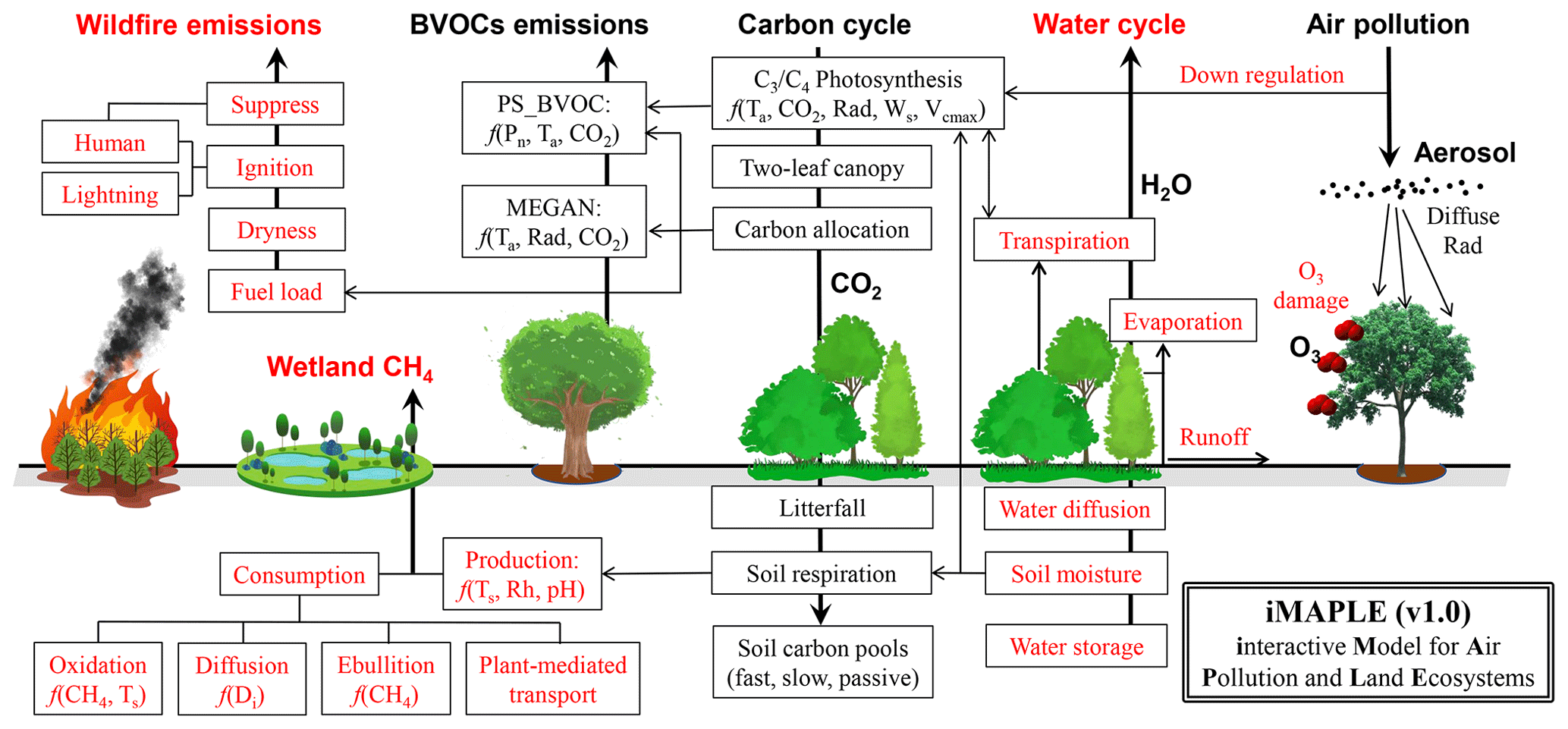
Figure 1 Illustration of biogeochemical processes in iMAPLE version 1.0. The carbon cycle is connected with the water cycle, wildfire emissions, biogenic volatile organic compounds (BVOCs) emissions, and wetland methane emissions and is affected by air pollutants including aerosols and ozone. The bold arrows indicate the directions of fluxes and air pollutants. The thin arrows indicate the influential pathways among different components. The dependences on key parameters are shown for some processes. Red font indicates new or updated processes in iMAPLE relative to the YIBs model. For detailed parameterizations please refer to Sect. 2.2.

2 Models and data

2.1 Main features of the YIBs model

The YIBs model is a process-based vegetation model predicting land carbon fluxes with dynamic changes in tree height, leaf area index, and carbon pools (Yue and Unger, 2015, hereafter YU2015). A total of nine plant functional types (PFTs) are considered including evergreen broadleaf forest (EBF), evergreen needleleaf forest (ENF), deciduous broadleaf forest (DBF), tundra, shrubland, ${\mathrm{C}}_{\mathrm{3}}/{\mathrm{C}}_{\mathrm{4}}$ grassland, and ${\mathrm{C}}_{\mathrm{3}}/{\mathrm{C}}_{\mathrm{4}}$ cropland. At each grid box, a mixture of PFTs with each PFT fraction is used as model input, sharing the temperature or moisture information from the same soil column. Leaf photosynthesis is calculated using the well-established Michaelis–Menten enzyme kinetics scheme (Farquhar et al., 1980) and is coupled to stomatal conductance with modulations of air humidity and CO₂ concentrations (Ball et al., 1987). The model applies a two-leaf approach to distinguish the irradiating states for sunlit and shading leaves and adopts an adaptive stratification for the radiative transfer processes within canopy layers (Spitters, 1986). The gross carbon assimilation is further regulated by the optimized plant phenology, which is mainly dependent on temperature and light for deciduous trees (Yue et al., 2015) but temperature and/or moisture for shrubland and grassland (YU2015). The assimilated carbon is allocated among the leaf, stem, and root to support autotrophic respiration and development, the latter of which is used to update plant height and leaf area (Cox, 2001). The input of litterfall triggers the carbon transition among 12 soil carbon pools and determines the magnitude of heterotrophic respiration with the joint effects of soil temperature, moisture, and texture (Schaefer et al., 2008). The net carbon uptake is then calculated by subtracting ecosystem respiration (plant and soil) and environmental perturbations (reforestation or deforestation) from the gross carbon assimilation (Yue et al., 2021). The YIBs model reasonably reproduces the observed spatiotemporal patterns of global carbon fluxes and makes contributions to the Global Carbon Project with long-term simulations of land carbon sink in the past century (Friedlingstein et al., 2020). The model specifically considers air pollution impacts on land ecosystems (Fig. 1), such as ozone vegetation damage (Yue and Unger, 2014) and the aerosol diffuse fertilization effect (Yue and Unger, 2017). YIBs implements two different schemes for BVOC emissions (Fig. 1), including the Model of Emissions of Gases and Aerosols from Nature (MEGAN, Guenther et al., 2012) and a photosynthesis-dependent (PS_BVOC) scheme (Unger et al., 2013).

2.2 New processes in iMAPLE

2.2.1 Process-based water cycles

The descriptions and units of all parameters used in this study are shown in Table S1 in the Supplement. We implement the hydrological module from Noah-MP into iMAPLE (Niu et al., 2011). The water budget closure is achieved by constructing water-balance equations among precipitation (P, $\mathrm{Kg}{\mathrm{m}}^{-\mathrm{2}}{\mathrm{s}}^{-\mathrm{1}}$), evapotranspiration (ET, $\mathrm{Kg}{\mathrm{m}}^{-\mathrm{2}}{\mathrm{s}}^{-\mathrm{1}}$), runoff, and terrestrial water storage change (ΔTWS) on each grid cell as follows:

$$\begin{array}{}\text{(1)}& P=\text{ET}+\text{runoff}+\mathrm{\Delta }\text{TWS}.\end{array}$$

Here, hourly P from MERRA-2 reanalyses is used as the input.

We then divide ET into three portions including plant transpiration (TRA), canopy evaporation (ECAN), and ground evaporation (EGRO):

$$\begin{array}{}\text{(2)}& \text{ET}=\text{TRA}+\text{ECAN}+\text{EGRO}.\end{array}$$

For vegetated grids, TRA is calculated as follows:

$$\begin{array}{}\text{(3)}& \text{TRA}={\displaystyle \frac{{\mathit{\rho }}_{\text{air}}\times {\text{CP}}_{\text{air}}\times C_{\text{tra}}\times (e_{\text{sat}}-e_{\text{ca}})}{\text{PC}}},\end{array}$$

where ρ_air is air density, CP_air is heat capacity of dry air, and PC is the psychrometric constant. e_sat is the saturated vapor pressure at the leaf temperature, e_ca is the vapor pressure of the canopy air, and C_tra is leaf transpiration conductance, which is calculated based on the Ball–Berry scheme of stomatal resistance (Yue and Unger, 2015). Meanwhile, ECAN is calculated as follows.

$$\begin{array}{}\text{(4)}& {\displaystyle }\text{ECAN}={\displaystyle \frac{{\mathit{\rho }}_{\text{air}}\times {\text{CP}}_{\text{air}}\times C_{\text{canopy,evap}}\times (e_{\text{sat}}-e_{\text{ca}})}{\text{PC}}}\text{(5)}& {\displaystyle }{C}_{\text{canopy,evap}}={\displaystyle \frac{f_{\text{wet}}\times E_{\text{VAI}}}{R_{\text{leaf,bdy}}}}\end{array}$$

Here, C_canopy,evap is the latent heat conductance from the wet leaf surface to canopy air. f_wet is the wet fraction of canopy, which is a fraction of the maximum canopy precipitation interception capacity. E_VAI is the effective vegetation area index and R_leaf,bdy is the bulk leaf boundary resistance. EGRO is calculated as follows:

$$\begin{array}{}\text{(6)}& \text{EGRO}=C_{\text{ground,evap}}(e_{\text{sat,ground}}\text{RH}-e_{\text{ca}}).\end{array}$$

Here, C_ground,evap is the coefficient for latent heat at the ground, e_sat,ground is the saturated vapor pressure at the ground, and RH is the surface relative humidity.

Runoff includes surface (R_srf) and subsurface (R_sub) components:

$$\begin{array}{}\text{(7)}& \text{runoff}=R_{\text{srf}}+R_{\text{sub}}.\end{array}$$

The surface runoff is calculated as follows:

$$\begin{array}{}\text{(8)}& R_{\text{srf}}=Q_{\text{soil,srf}}-Q_{\text{soil,in}},\end{array}$$

where Q_soil,srf is the incident water in the soil surface and is the sum of the precipitation, snowmelt, and dewfall. Q_soil,in is the infiltration into the soil, which is derived from approximate solutions of Richards equations with considerations of the spatial variations in precipitation and infiltration capacity. Here, we assume exponential distributions of infiltration capacity in each grid cell following the approach by Schaake et al. (1996).

$$\begin{array}{}\text{(9)}& {\displaystyle }{Q}_{\text{soil,in}}=Q_{\text{soil,srf}}{\displaystyle \frac{I_{\mathrm{c}}}{Q_{\text{soil,srf}}\mathrm{\Delta }t+I_{\mathrm{c}}}}\text{(10)}& {\displaystyle }{I}_{\mathrm{c}}=W_{\mathrm{d}}[\mathrm{1}-\exp (-K_{\mathrm{\Delta }t}\mathrm{\Delta }t\left)\right]\end{array}$$

Here, I_c and W_d are the soil infiltration capacity of the model grid cell and the water deficit of the soil column, respectively. K_Δt and Δt are the calibratable parameters and model time step. We assume free drainage processes in the soil column bottom, and thus the R_sub is calculated as follows:

$$\begin{array}{}\text{(11)}& R_{\text{sub}}={\mathit{\alpha }}_{\text{slope}}\times K_{\mathrm{4}},\end{array}$$

where α_slope=0.1 is the terrain slope index. K₄ is the hydraulic conductivity in the bottom soil layer parameterized following the scheme in Clapp and Hornberger (1978) and is calculated using spatial soil profiles from Hengl et al. (2017).

Terrestrial water storage (TWS) is the sum of groundwater storage (W_gw), soil water content (W_soil), and snow water equivalent (W_snow):

$$\begin{array}{}\text{(12)}& \text{TWS}=W_{\text{gw}}+W_{\text{snow}}+\sum _{i=\mathrm{1}}^{N_{\text{soil}}}{W}_{\text{soil}}.\end{array}$$

Here, the soil module includes four layers (N_soil=4) and W_soil is calculated by the volumetric water content (W_i) as follows:

$$\begin{array}{}\text{(13)}& W_{\text{soil}}={\mathit{\rho }}_{\text{wat}}\times W_i\times \mathrm{\Delta }{Z}_i\mathrm{\text{for }}i=\mathrm{1},\mathrm{2},\mathrm{3},\mathrm{4},\end{array}$$

where water density (ρ_wat)=1000 kg m⁻³, and ΔZ_i=0.1, 0.3, 0.6, and 1 m. Hourly W_i depends on variations of soil water diffusion (D) and hydraulic conductivity (K) as follows:

$$\begin{array}{}\text{(14)}& {\displaystyle \frac{\partial W}{\partial t}}={\displaystyle \frac{\partial }{\partial z}}\left(D{\displaystyle \frac{\partial W}{\partial z}}\right)+{\displaystyle \frac{\partial K}{\partial z}}.\end{array}$$

Here, K and D are calculated following the parameterizations of Clapp–Hornberger curves (Clapp and Hornberger, 1978):

$$\begin{array}{}\text{(15)}& {\displaystyle \frac{K}{K_{\text{sat}}}}={\left({\displaystyle \frac{W}{W_{\text{sat}}}}\right)}^{\mathrm{2}b+\mathrm{3}},\text{(16)}& {\displaystyle }D=K\times {\displaystyle \frac{\partial \mathit{\phi }}{\partial W}},\text{(17)}& {\displaystyle \frac{\mathit{\phi }}{{\mathit{\phi }}_{\text{sat}}}}={\left({\displaystyle \frac{W}{W_{\text{sat}}}}\right)}^{-b},\end{array}$$

where φ_sat, W_sat, and K_sat are saturated soil capillary potential, volumetric water content, and hydraulic conductivity. Exponent b is an empirical constant depending on soil types. Soil moisture is calculated as the ratio of W_s to W_sat.

Soil temperature (T_s) is calculated through physical processes as follows:

$$\begin{array}{}\text{(18)}& {\displaystyle \frac{\partial T_{\mathrm{s}}}{\partial t}}={\displaystyle \frac{\mathrm{1}}{C}}{\displaystyle \frac{\partial }{\partial z}}\left(K_T{\displaystyle \frac{\partial T_{\mathrm{s}}}{\partial z}}\right).\end{array}$$

Here K_T is soil specific heat capacity,

$$\begin{array}{}\text{(19)}& K_T=K_e\times \left(K_{\mathrm{s}}-K_{\text{dry}},\right)+K_{\text{dry}}\end{array}$$

where K_e, K_s, and K_dry are Kersten values as a function of soil wetness, saturated soil heat conductivity, and that under dry air conditions (Niu et al., 2011). C in Eq. (13) is the specific heat:

$$\begin{array}{}\text{(20)}& {\displaystyle }\begin{array}{rl}{\displaystyle }C=& {\displaystyle }{W}_{\text{lip}}\times C_{\text{lip}}+W_{\text{ice}}\times C_{\text{ice}}+(\mathrm{1}-W_{\text{sat}})\times C_{\text{sat}}\\ {\displaystyle }& {\displaystyle }+(W_{\text{sat}}-W)\times C_{\text{air}}.\end{array}\end{array}$$

Here, W_lip, C_lip, and W_ice, C_ice indicate water content and heat capacity on soil water and ice. C_sat and C_air are saturated and air heat capacity, which are empirical constants (Niu et al., 2011).

2.2.2 Dynamic fire emissions

We implement the active global fire parameterizations from Pechony and Shindell (2009) and Li et al. (2012) to iMAPLE. The fire emissions are determined by several key factors such as fuel flammability, natural ignitions, human activities, and fire spread. The fire count N_fire depends on flammability (Flam), fire ignition (including both natural ignition rate I_N and anthropogenic ignition rate I_A), and anthropogenic suppression (F_NS):

$$\begin{array}{}\text{(21)}& N_{\text{fire}}=\text{Flam}\times (I_{\mathrm{N}}+I_{\mathrm{A}})\times F_{\text{NS}}.\end{array}$$

Flam is a unitless metric representing conditions conducive to fire occurrence. It is parameterized as a function of vapor pressure deficit (VPD), precipitation (Prec), and leaf area index (LAI):

$$\begin{array}{}\text{(22)}& \text{Flam}=\text{VPD}\times e^{-\mathrm{2}\times \text{Prec}}\times \text{LAI}.\end{array}$$

I_N depends on the cloud-to-ground lightning, and I_A can be expressed as

$$\begin{array}{}\text{(23)}& I_{\mathrm{A}}=\mathrm{0.03}\times \text{PD}\times k\left(\text{PD}\right),\end{array}$$

where PD is population density. The empirical function of $k\left(\text{PD}\right)=\mathrm{6.8}\times {\text{PD}}^{-\mathrm{0.6}}$ stands for ignition potential by human activity. The fraction of non-suppressed fires F_NS is derived as

$$\begin{array}{}\text{(24)}& F_{\text{NS}}=\mathrm{0.05}+\mathrm{0.95}\times e^{-\mathrm{0.05}\times \text{PD}}.\end{array}$$

The burned area of a single fire (BA_single) is typically taken to be elliptical in shape associated with length-to-breadth ratio (LB), head-to-back ratio (HB), and rate of fire spread (UP) as follows:

$$\begin{array}{}\text{(25)}& {\text{BA}}_{\text{single}}={\displaystyle \frac{\mathit{\pi }\times {\text{UP}}^{\mathrm{2}}}{\mathrm{4}\times \text{LB}}}\times {\left(\mathrm{1}+{\displaystyle \frac{\mathrm{1}}{\text{HB}}}\right)}^{\mathrm{2}}.\end{array}$$

Then, LB and HB are related to changes in near-surface wind speed (U) as follows.

$$\begin{array}{}\text{(26)}& {\displaystyle }\text{LB}=\mathrm{1}+\mathrm{10}\times (\mathrm{1}-e^{-\mathrm{0.06}\times U})\text{(27)}& {\displaystyle }\text{HB}={\displaystyle \frac{\text{LB}+({\text{LB}}^{\mathrm{2}}-\mathrm{1}{)}^{\mathrm{0.5}}}{\text{LB}-({\text{LB}}^{\mathrm{2}}-\mathrm{1}{)}^{\mathrm{0.5}}}}\end{array}$$

Meanwhile, UP is computed as the function of relative humidity (RH):

$$\begin{array}{}\text{(28)}& \text{UP}={\text{UP}}_{\text{max}}\times f_{\text{RH}}\times f_{\mathit{\theta }}\times G\left(U\right).\end{array}$$

Here, UP_max is the maximum fire spread rate depending on PFTs, and f_RH and f_θ represent the dependence of fire spread on RH and on root-zone soil moisture, respectively. f_θ is simply set to 0.5, and f_RH is calculated as

$$\begin{array}{}\text{(29)}& f_{\text{RH}}=\left\{\begin{array}{ll}\mathrm{1},& \text{RH}\le {\text{RH}}_{\text{low}}\\ {\displaystyle \frac{{\text{RH}}_{\mathrm{up}}-\text{RH}}{{\text{RH}}_{\text{up}}-{\text{RH}}_{\text{low}}}},{\text{RH}}_{\text{low}}<& \text{RH}<{\text{RH}}_{\text{up}}\\ \mathrm{0},& \text{RH}\ge {\text{RH}}_{\text{up}}.\end{array}\right.\end{array}$$

In this study, we set RH_low=30 % and RH_up=70 % as the lower and upper thresholds of RH following the methods used in Li et al. (2012). If RH is higher than 70 %, natural fires will not occur or spread, and RH will no longer be a constraint for fire occurrence and spread if RH ≤ 30 %. G(U) is the limit of the fire spread:

$$\begin{array}{}\text{(30)}& G\left(U\right)={\displaystyle \frac{\text{LB}}{\mathrm{1}+\frac{\mathrm{1}}{\text{HB}}}}.\end{array}$$

In general, the eccentricity of burned area is primarily influenced by near-surface wind speed, while the rate of fire spread is jointly regulated by near-surface wind speed and relative humidity. The shape of the fire is converted to a circular form when the near-surface wind speed reaches zero, and burning ceases to propagate once the relative humidity is above a specific threshold. The dependence of BA_single on U and RH is shown in Fig. S1 in the Supplement.

Finally, the burned area (BA) is represented as

$$\begin{array}{}\text{(31)}& \text{BA}={\text{BA}}_{\text{single}}\times N_{\text{fire}}.\end{array}$$

The fire-emitted trace gases and aerosols (Emis) are calculated as

$$\begin{array}{}\text{(32)}& \text{Emis}=\text{BA}\times \text{EF},\end{array}$$

where EF is the emission factors for different species (such as black carbon and organic carbon aerosols). It is important to note that the feedbacks from fire activities onto the terrestrial ecosystem have not been considered in the current version of iMAPLE due to the high complexity.

2.2.3 Wetland methane emissions

We implement process-based wetland CH₄ emissions into iMAPLE. The anthropogenic sources of CH₄ from Phase 6 of the Coupled Model Intercomparison Project (CMIP6, https://aims2.llnl.gov/search/input4MIPs/, last access: 5 June 2024) are also used as input for iMAPLE. For each soil layer, the flux of CH₄ ($F_{{\mathrm{CH}}_{\mathrm{4}}}$) is calculated as the difference between production ($P_{{\mathrm{CH}}_{\mathrm{4}}}$) and consumption, which includes oxidation ($O_{{\mathrm{CH}}_{\mathrm{4}}}$), ebullition ($E_{{\mathrm{CH}}_{\mathrm{4}}}$), diffusion ($D_{{\mathrm{CH}}_{\mathrm{4}}}$), and plant-mediated transport through aerenchyma ($A_{{\mathrm{CH}}_{\mathrm{4}}}$) as follows:

$$\begin{array}{}\text{(33)}& F_{{\mathrm{CH}}_{\mathrm{4}}}=P_{{\mathrm{CH}}_{\mathrm{4}}}-O_{{\mathrm{CH}}_{\mathrm{4}}}-E_{{\mathrm{CH}}_{\mathrm{4}}}-D_{{\mathrm{CH}}_{\mathrm{4}}}-A_{{\mathrm{CH}}_{\mathrm{4}}}.\end{array}$$

The net methane emission to the atmosphere is the sum of ebullition, diffusion, and aerenchyma transport from the top soil layer.

The production of CH₄ in soil depends on the quantity of carbon substrate and environmental conditions including soil temperature T_s, pH, and wetland inundation fraction f_wetland as follows:

$$\begin{array}{}\text{(34)}& P_{{\mathrm{CH}}_{\mathrm{4}}}=R_{\mathrm{h}}r{f}_{\text{Ts}}{f}_{\text{pH}}{f}_{\text{wetland}},\end{array}$$

where R_h is the heterotrophic respiration estimated at the grid cell ($\mathrm{mol}\mathrm{C}{\mathrm{m}}^{-\mathrm{2}}{\mathrm{s}}^{-\mathrm{1}}$). r represents the release ratio of methane and carbon dioxide (Wania et al., 2010). We determine the dependence on T_s and soil pH in iMAPLE based on the parameterizations from the TRIPLEX-GHG model (Zhu et al., 2014). The impact factor of soil temperature f_ST can be calculated as follows (Zhang et al., 2002; Zhu et al., 2014).

$$\begin{array}{}\text{(35)}& {\displaystyle }{f}_{\text{ST}}=\left\{\begin{array}{ll}\mathrm{0},& T_{\mathrm{s}}<T_{\text{min}}\\ {\text{vt}}^{\text{xt}}\exp \left(\text{xt}\right(\mathrm{1}-\text{vt}\left)\right),& T_{\text{min}}\le T_{\mathrm{s}}\le T_{\text{max}}\\ \mathrm{0},& T_{\mathrm{s}}>T_{\text{max}}\end{array}\right.\text{(36)}& {\displaystyle }\text{vt}=(T_{\text{max}}-T_{\mathrm{s}})/(T_{\text{max}}-T_{\text{opt}})\text{(37)}& {\displaystyle }\text{xt}=\left[\log \right(Q_{\mathrm{10}}\left)\right(T_{\text{max}}-T_{\text{opt}}\left){]}^{\mathrm{2}}\right(\mathrm{1.0}+{\text{at}}^{\mathrm{0.5}}{)}^{\mathrm{2}}/\mathrm{400.0}\text{(38)}& {\displaystyle }\text{at}=\mathrm{1.0}+\mathrm{40.0}/\left[\log \right(Q_{\mathrm{10}}\left)\right(T_{\text{max}}-T_{\text{opt}}\left)\right]\end{array}$$

T_min, T_max, and T_opt represent the lowest, highest, and optimum temperature for the process of methane production and oxidation, respectively. In this study, T_min=0 °C, T_max=45 °C, and T_opt=25 °C (Zhu et al., 2014).

For the temperature dependence, the Q₁₀ relationships are applied as follows:

$$\begin{array}{}\text{(39)}& Q_{\mathrm{10}}=r_{\mathrm{b}}{Q}_{\mathrm{b}}^{\frac{T_{\mathrm{s}}-T_{\text{base}}}{\mathrm{10}}}.\end{array}$$

Here r_b is set to 3.0 and Q_b is 1.33 with a base temperature (T_base) of 25 °C (Zhu et al., 2014; Paudel et al., 2016). The inundation fraction of wetland at each cell describes the proportion of anaerobic conditions (Zhang et al., 2021). We ignore the impact of redox potential (Eh) because global observations are not available and the Eh-related processes are poorly characterized in current models (Wania et al., 2010).

The oxidation of CH₄ is a series of aerobic activities related to temperature and CH₄ concentrations:

$$\begin{array}{}\text{(40)}& O_{{\mathrm{CH}}_{\mathrm{4}}}=\left[{\mathrm{CH}}_{\mathrm{4}}\right]f_{\text{Ts}}{f}_{{\mathrm{CH}}_{\mathrm{4}}},\end{array}$$

where [CH₄] is the methane amount in each soil layer (g C m⁻² per layer). $f_{{\mathrm{CH}}_{\mathrm{4}}}$ is the CH₄ concentration factor representing a Michaelis–Menten kinetic relationship:

$$\begin{array}{}\text{(41)}& f_{{\mathrm{CH}}_{\mathrm{4}}}={\displaystyle \frac{\left[{\mathrm{CH}}_{\mathrm{4}}\right]}{\left[{\mathrm{CH}}_{\mathrm{4}}\right]+K_{{\mathrm{CH}}_{\mathrm{4}}}}},\end{array}$$

where $K_{{\mathrm{CH}}_{\mathrm{4}}}=\mathrm{5}$ µmol L⁻¹ is the half-saturation coefficient with respect to CH₄ (Walter and Heimann, 2000). For temperature dependence of oxidation, the Q₁₀ relationship with r_b=2.0, Q_b=1.9, and T_base=12 °C is adopted (Zhu et al., 2014; Paudel et al., 2016).

The diffusion of CH₄ follows Fick's law with dependence on CH₄ concentrations and the molecular diffusion coefficients of CH₄ in the air (D_a=0.2 cm² s⁻¹) and water (D_w=0.00002 cm² s⁻¹), respectively (Walter and Heimann, 2000). For each soil layer i, the diffusion coefficient D_i can be calculated as follows:

$$\begin{array}{}\text{(42)}& {\displaystyle }\begin{array}{rl}{\displaystyle }{D}_i=& {\displaystyle }{D}_{\mathrm{a}}\times (R_{\text{sand}}\times \mathrm{0.45}+R_{\text{silt}}\times \mathrm{0.2}+R_{\text{clay}}\times \mathrm{0.14})\\ {\displaystyle }& {\displaystyle }\times f_{\text{tort}}\times S_{\text{poro}}\times (\mathrm{1}-{\text{WFPS}}_i)+D_{\mathrm{w}}\times {\text{WFPS}}_i,\end{array}\end{array}$$

where R_sand, R_silt, and R_clay are the relative content of sand, silt, and clay in the soil, f_tort=0.66 is the tortuosity coefficient, S_poro is soil porosity, and WFPS represents the pore space full of water (Zhuang et al., 2004).

The ebullition of CH₄ occurs when the CH₄ concentration is above the threshold of 0.5 mol CH₄ m⁻³ (Walter et al., 2001). Since the process of ebullition occurs in a very short time, the bubbles will generate at once and all the flux will be released to the atmosphere if the concentration reaches the threshold. The plant-mediated transport of CH₄ through aerenchyma is dependent on the concentration gradient of CH₄ and plant-related factors (Zhu et al., 2014). The $A_{{\mathrm{CH}}_{\mathrm{4}}}$ is determined by the oxidation factor for roots and the aerenchyma factor for plants. The baseline value of the oxidation factor in roots is 0.5, with a regulatory range from 0.2 to 1.0 determined by the wetland plant types. The plant aerenchyma factor is calculated by the ratio of the plant root length density (typical value: 2.1 cm mg⁻¹) and the root cross-sectional area (typical value: 0.0013 cm²), along with a plant root to atmosphere diffusion factor for methane which is modulated by plant type within a range of 0 to 1 (Zhang et al., 2002).

2.2.4 The downregulation on photosynthesis

We implement the downregulation parameterization from Arora et al. (2009) to indicate the nutrient limitations on leaf photosynthesis. A downregulating factor ε is calculated as a function of CO₂ concentrations (C) as follows:

$$\begin{array}{}\text{(43)}& \mathit{\epsilon }\left(C\right)={\displaystyle \frac{\mathrm{1}+{\mathit{\gamma }}_{\text{gd}}\ln (C/C_{\mathrm{0}})}{\mathrm{1}+{\mathit{\gamma }}_g\ln (C/C_{\mathrm{0}})}},\end{array}$$

where C₀ is a reference CO₂ concentration set to 288 ppm. The values of γ_gd=0.42 and γ_g=0.90 are derived from multiple measurements to constrain the CO₂ fertilization. Then the downregulated photosynthesis is calculated by scaling the original value with the factor of ε.

2.2.5 Trait-based O₃ vegetation damaging scheme

The YIBs model considers O₃ vegetation damage using the flux-based scheme proposed by Sitch et al. (2007) (hereafter S2007), which determines the damaging ratio F of plant photosynthesis as follows:

$$\begin{array}{}\text{(44)}& F=a_{\text{PFT}}\times max\mathit{\{}{f}_{{\mathrm{O}}_{\mathrm{3}}}-t_{\text{PFT}},\mathrm{0}\mathit{\}}.\end{array}$$

Here, $f_{{\mathrm{O}}_{\mathrm{3}}}$ denotes O₃ stomatal flux ($\mathrm{nmol}{\mathrm{m}}^{-\mathrm{2}}{\mathrm{s}}^{-\mathrm{1}}$) defined as

$$\begin{array}{}\text{(45)}& f_{{\mathrm{O}}_{\mathrm{3}}}={\displaystyle \frac{\left[{\mathrm{O}}_{\mathrm{3}}\right]}{r+\left[\frac{k_{{\mathrm{O}}_{\mathrm{3}}}}{g_{\mathrm{p}}\times (\mathrm{1}-F)}\right]}},\end{array}$$

where [O₃] represents the O₃ concentrations at the reference level (nmol m⁻³). r is the sum of boundary and aerodynamic resistance between the leaf surface and reference level (s m⁻¹). g_p is the potential stomatal conductance for H₂O (m s⁻¹). $k_{{\mathrm{O}}_{\mathrm{3}}}=\mathrm{1.67}$ is a conversion factor of leaf resistance for O₃ to that for water vapor. The level of O₃ damage is then determined by the PFT-specific sensitivity a_PFT and threshold t_PFT, which are different among PFTs.

In iMAPLE, we implement the trait-based O₃ vegetation damaging scheme to unify the inter-PFT sensitivities (Ma et al., 2023):

$$\begin{array}{}\text{(46)}& a_{\text{PFT}}={\displaystyle \frac{a}{\text{LMA}}}.\end{array}$$

Here, a unified plant sensitivity a (nmol⁻¹ g s) is scaled by leaf mass per area (LMA, g m⁻²) to derive the sensitivity of a specific PFT (a_PFT). Accordingly, the damaging fraction F is modified as follows:

$$\begin{array}{}\text{(47)}& F=a\times max\left\{{\displaystyle \frac{f_{{\mathrm{O}}_{\mathrm{3}}}}{\text{LMA}}}-t,\mathrm{0}\right\}.\end{array}$$

Here t ($\mathrm{nmol}{\mathrm{g}}^{-\mathrm{1}}{\mathrm{s}}^{-\mathrm{1}}$) is a unified flux threshold for O₃ vegetation damage. The $f_{{\mathrm{O}}_{\mathrm{3}}}$ in Eq. (45) is fed into Eq. (47) to build a quadratic equation for F. We solve the quadratic equation and select the F value within the range of [0,1]. The updated scheme considers the dilution effects of O₃ dose through leaf cross-section by incorporating LMA. Plants with high LMA (e.g., ENF and EBF) usually have low sensitivities, and those with low LMA (e.g., DBF and crops) are more sensitive to O₃ damage. The unified sensitivity a is set to 3.5 nmol⁻¹ g s and threshold t is set to 0.019 $\mathrm{nmol}{\mathrm{g}}^{-\mathrm{1}}{\mathrm{s}}^{-\mathrm{1}}$ by calibrating simulated F values with literature-based measurements (Ma et al., 2023).

2.3 Design of simulations

We perform four sensitivity experiments with iMAPLE. The baseline (BASE) simulation considers the two-way coupling between carbon and water cycles so that the prognostic soil meteorology drives canopy photosynthesis and evapotranspiration. A sensitivity run named BASE_NW is set up by turning off the water cycle in iMAPLE. In this simulation, the soil moisture and soil temperature are adopted from the Modern-Era Retrospective Analysis for Research and Applications, Version 2 (MERRA-2) reanalyses (Gelaro et al., 2017). The third and fourth runs turn on the O₃ vegetation damage effect using either the LMA-based scheme (O3LMA) or the S2007 scheme (O3S2007). Surface hourly O₃ concentrations are adopted from the chemical transport model simulations used in our previous study (Yue and Unger, 2018). For all simulations, iMAPLE is driven with hourly surface meteorology at a spatial resolution of 1° × 1° from the MERRA-2 reanalyses, including surface air temperature, air pressure, specific humidity, wind speed, precipitation, snowfall, and shortwave and longwave radiation. We run the model for the period of 1980–2021 using the initial conditions of the equilibrium soil carbon pool, tree height, and water fluxes from a spin-up run of 200 years driven with perpetual forcing for the year 1980.

iMAPLE is driven with observed CO₂ concentrations from Mauna Loa (Keeling et al., 1976) and the land cover fraction of nine PFTs derived by combining satellite retrievals from both the Moderate Resolution Imaging Spectroradiometer (MODIS) (Hansen et al., 2003) and Advanced Very High Resolution Radiometer (AVHRR) (Defries et al., 2000). For fire emissions, we use Gridded Population of the World version 4 (https://sedac.ciesin.columbia.edu/data/collection/gpw-v4, last access: 5 June 2024) to calculate human ignition and suppression. The lightning ignition is calculated using the flash rate from the Very High Resolution Gridded Lightning Climatology Data Collection Version 1 (https://ghrc.nsstc.nasa.gov/uso/ds_details/collections/lisvhrcC.html, last access: 5 June 2024). For wetland CH₄ emissions, we use the 2000–2020 global dataset of Wetland Area and Dynamics for Methane Modeling (WAD2M) derived from static datasets and remote sensing (Zhang et al., 2021), global soil pH from Hengl et al. (2017), and gridded soil texture from Scholes et al. (2011). For the LMA-based O₃ damage scheme, we use gridded LMA from the trait-level dataset of TRY (Kattge et al., 2011) developed by extending field measurements with a random forest model (Moreno-Martínez et al., 2018).

2.4 Data for validations

We use observational datasets to validate the biogeochemical processes and related variables simulated by iMAPLE. For simulated carbon and water fluxes, site-level observations are collected from 201 sites from FLUXNET (Table S2 in the Supplement and Fig. 2). Among these sites, 95 have the ENF tree species as the major PFT and 106 are dominated by non-tree species, especially shrubland. Most (71 %) of the sites are located at the middle latitudes (30–60° N) of the Northern Hemisphere (NH), especially in the US and Europe. Compared to the previous evaluation in YU2015, we have many more sites in the tropics (22 in this study vs. 5 in YU2015), Asia (20 in this study vs. 1 in YU2015), and the Southern Hemisphere (28 in this study vs. 7 in YU2015) in this study. We also use the global gridded observations of GPP from the satellite retrievals including the solar-induced chlorophyll fluorescence (SIF) product GOSIF (Li and Xiao, 2019) and the Global Land Surface Satellite (GLASS) product (Yuan et al., 2010). The global observations of ET are adopted from the benchmark product of FLUXCOM (Jung et al., 2020) and the satellite-based GLASS product. For the dynamic fire module, we use monthly observed area burned from the Global Fire Emission Database version 4.1 with small fires (GFED4.1s) during 1997–2016 (van der Werf et al., 2010; Randerson et al., 2012). For methane emissions, we use site-level measurements of CH₄ fluxes from FLUXNET-CH₄ (Delwiche et al., 2021). We exclude monthly records with missing data for more than half of the days and calculate the long-term mean fluxes for the seasonal cycle. In total, we select 44 sites with at least 6 months of data available for the validations (Table S3 in the Supplement).

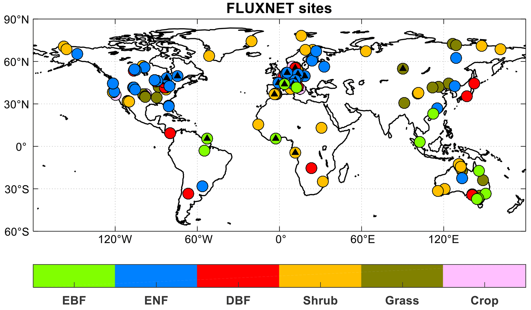
Figure 2 Spatial distributions of 201 sites from global FLUXNET. The colors indicate various plant functional types (PFTs) including evergreen broadleaf forest (EBF, 13 sites), evergreen needleleaf forest (ENF, 57 sites), deciduous broadleaf forest (DBF, 25 sites), shrub (52 sites), grass (37 sites), and crop (17 sites). The black triangles indicate sites with at least 1 year of observations of diffuse radiation.

3 Model evaluations

3.1 Site-level evaluations

Simulated GPP shows correlation coefficients (R) of 0.59–0.86 for the six main PFTs with varied sample numbers (Fig. 3). The highest R is achieved for ENF, though the model underestimates the mean GPP magnitude by 20.62 % for this species. On average, simulated GPP is lower than observations for most PFTs. Compared to previous evaluation of the YIBs model (YU2015), iMAPLE with coupled water cycle improves the R of GPP simulations for ENF (from 0.65 to 0.86) and grassland (from 0.7 to 0.8) but worsens the predictions for other species such as EBF (from 0.65 to 0.59). The main cause of this degradation is the application of MERRA-2 reanalyses in the iMAPLE simulations instead of the site-level meteorology used in YU2015. The biases in the meteorological input may cause uncertainties in the simulation of GPP fluxes (Ma et al., 2021). In addition, the mismatch of vegetation cover and soil properties between the site location and the 1° × 1° grid in the simulation may further contribute to the modeling biases.

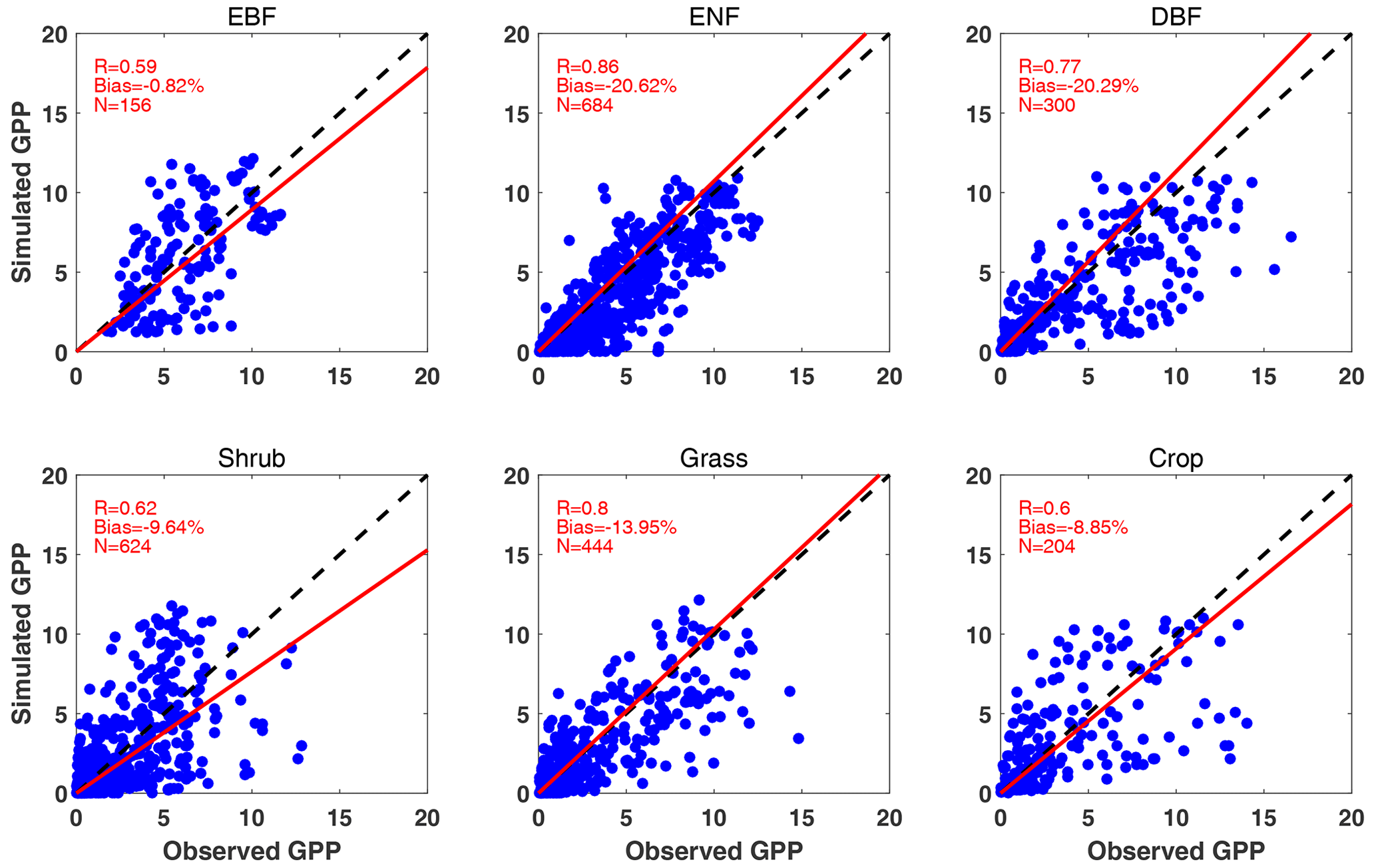
Figure 3 Comparisons between observed and simulated monthly GPP from 201 FLUXNET sites. Each point indicates the average value of 1 month at a site. The red line represents linear regression between observations and simulations from the BASE experiment. The correlation coefficient (R), normalized mean bias, and numbers of samples (N) are shown in each panel. The comparisons are grouped into six PFTs including EBF, ENF, DBF, shrub, grass, and crop. The unit is $\mathrm{g}\mathrm{C}{\mathrm{m}}^{-\mathrm{2}}{\mathrm{d}}^{-\mathrm{1}}$.

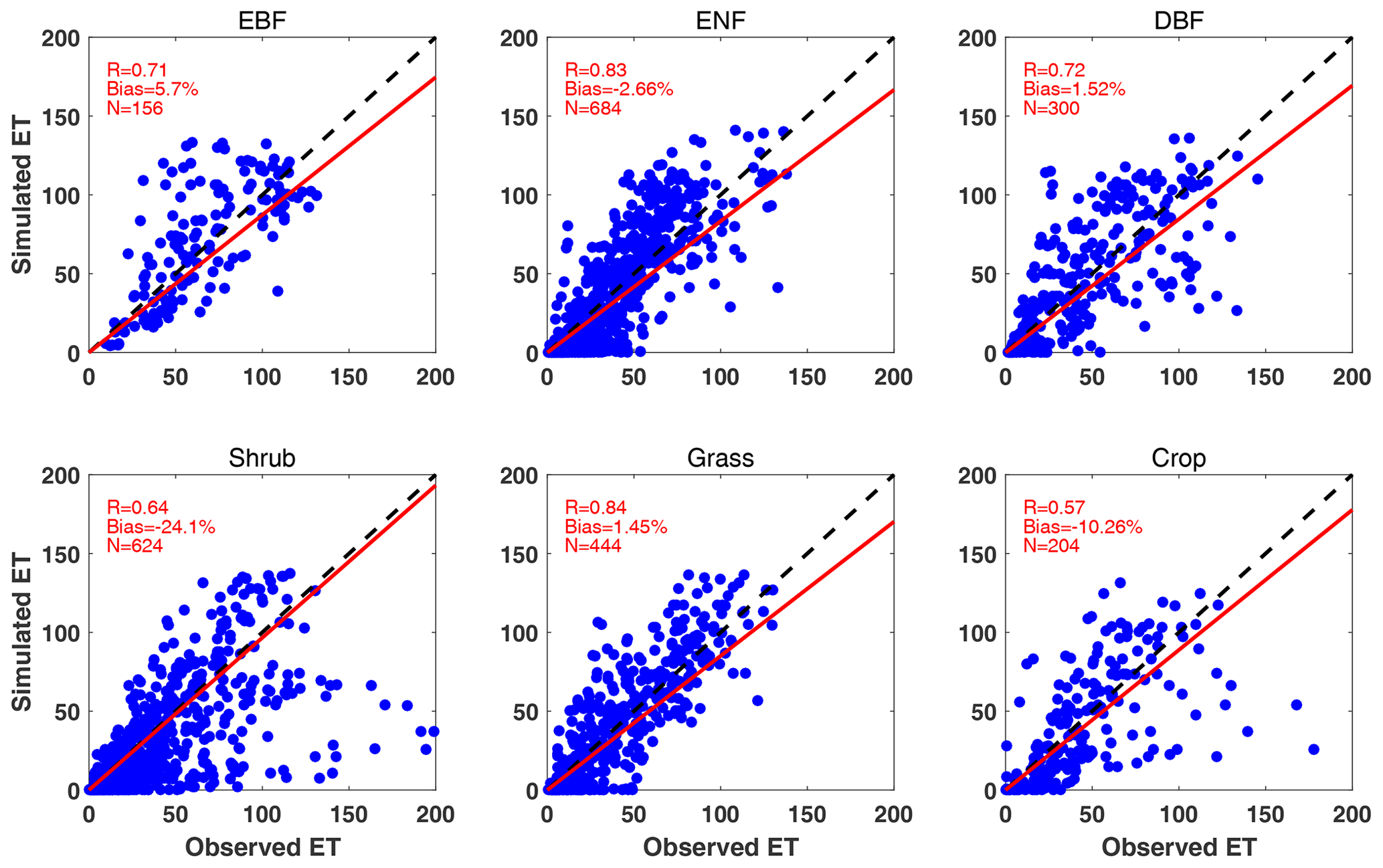
Simulated ET matches observations with correlation coefficients of 0.57–0.84 at the FLUXNET sites (Fig. 4). Relatively better performance is achieved for ENF (R=0.83) and grassland (R=0.84), for which the model yields good predictions of GPP as well. In contrast, low correlations and high biases are predicted for shrubland and cropland. For the shrubland sites, different land types (e.g., closed shrublands, permanent wetlands, and woody savannas) share the same parameters in iMAPLE, resulting in the biases in depicting the site-specific carbon and water fluxes. For cropland, the prognostic phenology of grass species is applied in the model due to the missing plantation information for individual sites. Even with these deficits, iMAPLE in general captures the spatiotemporal variations of GPP and ET at most sites.

Figure 4 The same as Fig. 3 but for ET. The unit is mm month⁻¹.

We further compare the simulated wetland CH₄ fluxes from the BASE experiment with observations at the FLUXNET-CH₄ sites. Similar to the carbon flux sites, most of these CH₄ flux sites are located in the NH (Fig. 5a). However, different from the carbon fluxes which usually range from 0 to 15 $\mathrm{g}\mathrm{C}{\mathrm{m}}^{-\mathrm{2}}{\mathrm{d}}^{-\mathrm{1}}$, the CH₄ fluxes show a wide range across several orders of magnitude from 10⁻² to 10³ $\mathrm{g}\left[{\mathrm{CH}}_{\mathrm{4}}\right]{\mathrm{m}}^{-\mathrm{2}}{\mathrm{yr}}^{-\mathrm{1}}$ (Fig. 5b). Such a large contrast requires a more realistic configuration of model parameters to distinguish the large gradient among sites. For example, US-Tw1 and US-Tw4 are two nearby sites within a distance of 1 km, where our simulations give a CH₄ flux of 14.35 $\mathrm{g}\left[{\mathrm{CH}}_{\mathrm{4}}\right]{\mathrm{m}}^{-\mathrm{2}}{\mathrm{yr}}^{-\mathrm{1}}$ during 2011–2017. However, the average CH₄ flux shows a difference of 3.7 times with 66.31 $\mathrm{g}\left[{\mathrm{CH}}_{\mathrm{4}}\right]{\mathrm{m}}^{-\mathrm{2}}{\mathrm{yr}}^{-\mathrm{1}}$ at US-Tw1 and 18.16 $\mathrm{g}\left[{\mathrm{CH}}_{\mathrm{4}}\right]{\mathrm{m}}^{-\mathrm{2}}{\mathrm{yr}}^{-\mathrm{1}}$ at US-Tw4 during 2011–2017. In the model, these two sites share the same land surface properties because they are located on the same grid. On average, simulated CH₄ fluxes are correlated with observations at a moderate R of 0.68 and a normalized mean bias (NMB) of −28 %.

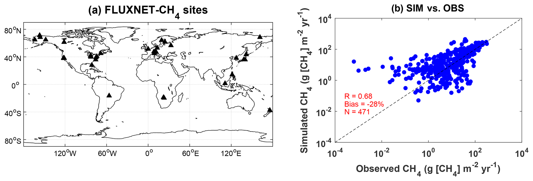
Figure 5 (a) Spatial distribution of global FLUXNET-CH₄ sites and (b) comparisons between observed and simulated monthly methane flux from the BASE experiment. Filled triangles indicate sites with at least 6 months of observations of wetland CH₄ fluxes. Each point represents an average value of monthly methane emission at one site. The correlation coefficient (R), normalized mean bias, and numbers of samples (N) are shown in the right panel. The unit is $\mathrm{g}\left[{\mathrm{CH}}_{\mathrm{4}}\right]{\mathrm{m}}^{-\mathrm{2}}{\mathrm{yr}}^{-\mathrm{1}}$.

3.2 Grid-level evaluations

The coupling of the Noah-MP module enables the dynamic prediction of soil parameters by iMAPLE. We compare the simulated soil moisture and soil temperature from the BASE experiment with MERRA-2 reanalyses (Fig. 6). Both simulations (Fig. 6a) and observations (Fig. 6b) show low soil moisture over arid and semiarid regions with the minimum in North Africa. The model also captures the high soil moisture in tropical rainforest. However, the prediction underestimates soil moisture in boreal regions in the NH (Fig. 6c). On the global scale, simulated soil moisture matches observations with a high R of 0.86 and a low NMB of −6.9 %. These statistical metrics are further improved for the simulated soil temperature with R of 0.99 and NMB of 0.5 % against observations (Fig. 6f). The simulation reproduces the observed spatial pattern with a uniform warming bias.

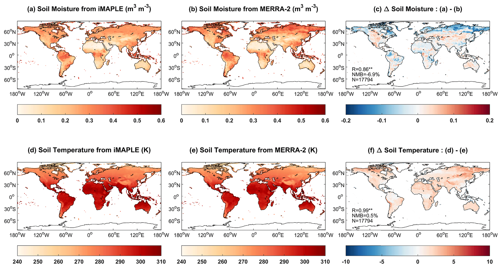
Figure 6 Comparisons of simulated (a) soil moisture (m³ m⁻³) and (d) soil temperature (K) from iMAPLE with (b, e) the MERRA-2 reanalyses. Both simulations from the BASE experiment and observations from MERRA-2 reanalyses are averaged for the period of 1980–2020. The spatial difference, correlation coefficient (R), normalized mean bias (NMB) between simulations and observations, and numbers of points (N) are shown in (c) and (f).

Driven with the prognostic soil moisture and temperature, iMAPLE predicts reasonable land carbon and water fluxes (Fig. 7). Simulated GPP (Fig. 7a) reproduces observed patterns (Fig. 7b) with high values in the tropical rainforest, moderate values in the boreal forests, and low values in the arid regions. On the global scale, our simulations yield a total GPP of 129.8 Pg C yr⁻¹, similar to the observed amount of 125.4 Pg C yr⁻¹. The predicted GPP is higher than observations over the tropical rainforest (Fig. 7c). However, such overestimation may instead be an indicator of biases in the ensemble observations, which are derived from the empirical models instead of direct measurements (Yuan et al., 2010; Running et al., 2004). Our site-level evaluations show that iMAPLE predicts reasonable GPP values at the EBF sites (Fig. 3). Despite this inconsistency, the model yields a high R of 0.92 and a small NMB of 1.3 % for GPP against observations on the global scale (Fig. 7c). Simulated ET (Fig. 7d) matches the observations (Fig. 7e) with high values in the tropical rainforest and secondary high values in the boreal forest. In general, the prediction is lower than observations except for the eastern US and eastern China (Fig. 7f). On average, iMAPLE shows R of 0.93 and NMB of −10.4 % in the simulation of ET compared to the ensemble of observations.

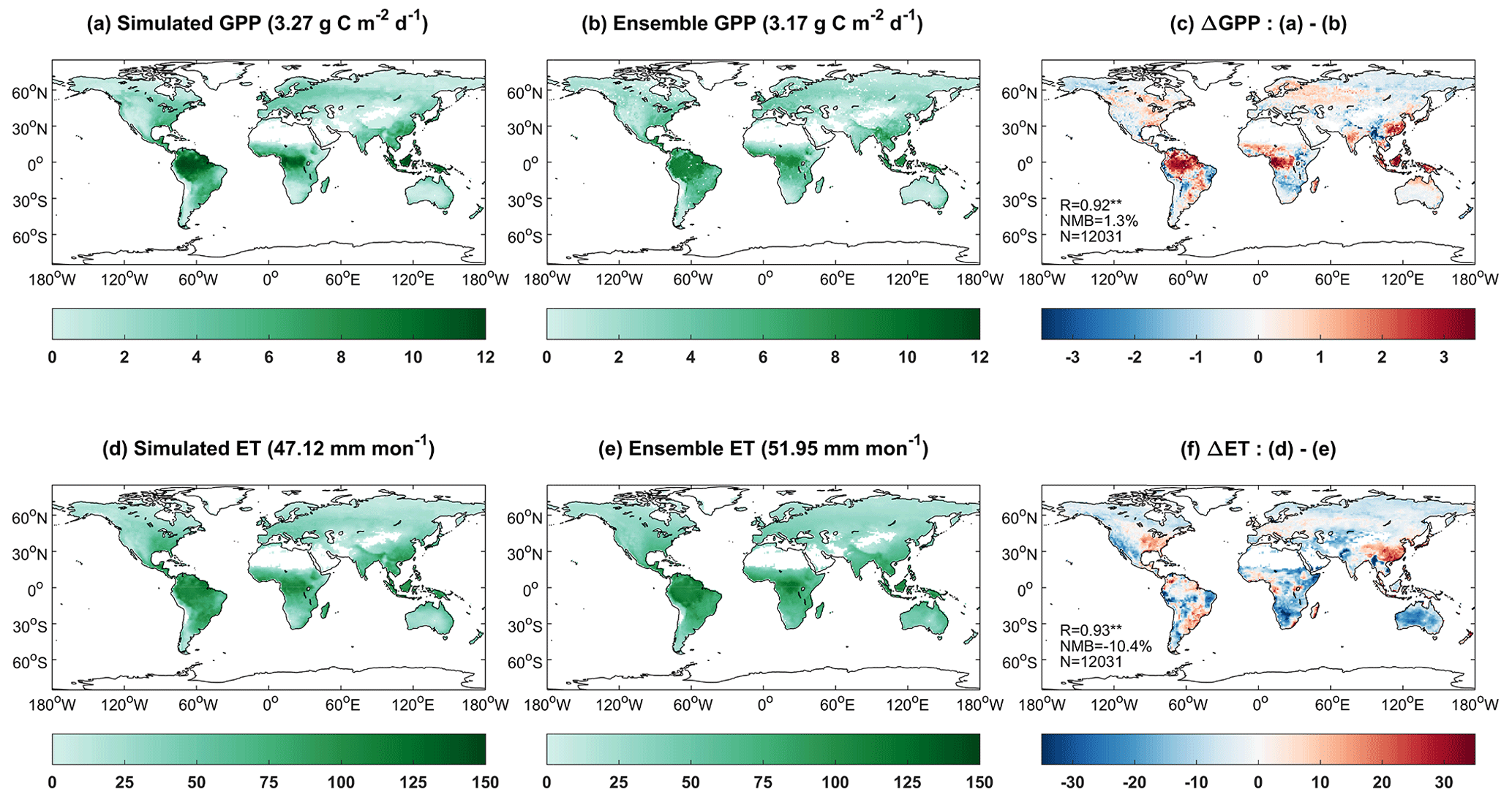
Figure 7 Comparisons of simulated (a) gross primary productivity (GPP, $\mathrm{g}\mathrm{C}{\mathrm{m}}^{-\mathrm{2}}{\mathrm{d}}^{-\mathrm{1}}$) and (d) evapotranspiration (ET, mm month⁻¹) with ensemble products from (b, e) observations. Simulated GPP and ET are performed by iMAPLE driven with meteorology from MERRA-2 reanalysis (BASE) during 2001–2013. Ensemble GPP products are from the average values of SIF-based GOSIF and satellite-based GLASS GPP products. Ensemble ET products include FLUXCOM and GLASS products during 2001–2013. The spatial difference, correlation coefficient (R), normalized mean bias (NMB) between simulations and observations, and numbers of points (N) are shown in (c) and (f). Only land grids with vegetation are shown in each panel, and their area-weighed values are shown in titles.

We further compare the simulated GPP with (BASE) or without (BASE_NW) a dynamic water cycle (Fig. 8). Relative to the simulations driven with MERRA-2 soil moisture and temperature, iMAPLE coupled with the Noah-MP water module predicts very similar GPP over the hotspot regions such as tropical rainforest and boreal forest (Fig. 8a). However, the coupled model predicts lower GPP for grassland in the tropics (e.g., South America and central Africa) but higher GPP in arid regions (e.g., South Africa and Australia). Since the baseline GPP is very low in arid regions, the relative changes are even larger than 100 % over those areas. These GPP differences are mainly driven by the changes in soil moisture, which increases over the arid regions with the dynamic water cycle (Fig. 6c). The reduction of soil moisture in the high latitudes of the NH shows limited impacts on the predicted GPP, likely because the boreal ecosystem is more dependent on temperature than moisture (Beer et al., 2010).

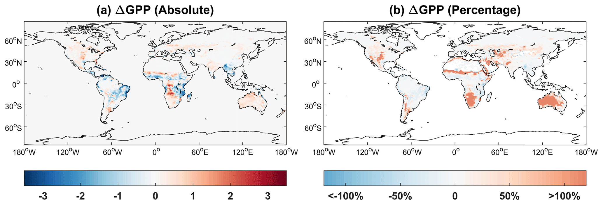
Figure 8 Absolute ($\mathrm{g}\mathrm{C}{\mathrm{m}}^{-\mathrm{2}}{\mathrm{d}}^{-\mathrm{1}}$) and relative (%) differences of global GPP between simulations with (BASE) and without (BASE_NW) two-way carbon–water coupling processes. Simulation results are averaged for the period of 1980–2020.

3.3 Ecosystem perturbations to air pollution

Within the iMAPLE framework, the land ecosystem perturbs atmospheric components through emissions from biomass burning, wetland CH₄, and BVOCs. We compare the simulated burned fraction and fire-emitted organic carbon (OC) emissions with observations from GFED4.1s (Fig. 9). The largest burned fraction is predicted over the Sahel region and the countries of Angola and Zambia, surrounding the low center of the Congo rainforest. Moderate burnings could be found in northern Australia and eastern South America. Most of these hotspots are located on grassland and shrubland in the tropics, where the high temperature and limited rainfall promote regional fire activities. The model reasonably captures the observed fire pattern with a spatial correlation of 0.66 and NMB of 6.05 % (Fig. 9c), though the model overestimates the area burned in southern Africa. The predicted fire area is used to derive biomass burning emissions of air pollutants (e.g., carbon monoxide, nitrogen oxides, black carbon, organic carbon, and sulfur dioxide) with the specific emission factors (Tian et al., 2023). Furthermore, we compare fire-emitted OC from the model with GFED4.1s. The spatial pattern of OC emissions is similar to that of burned area. The simulations yield a total of 16.8 Tg yr⁻¹ for the global fire-emitted OC, slightly higher than the amount of 16.4 Tg yr⁻¹ from GFED4.1s with some overestimations in tropical Africa (Fig. 9f).

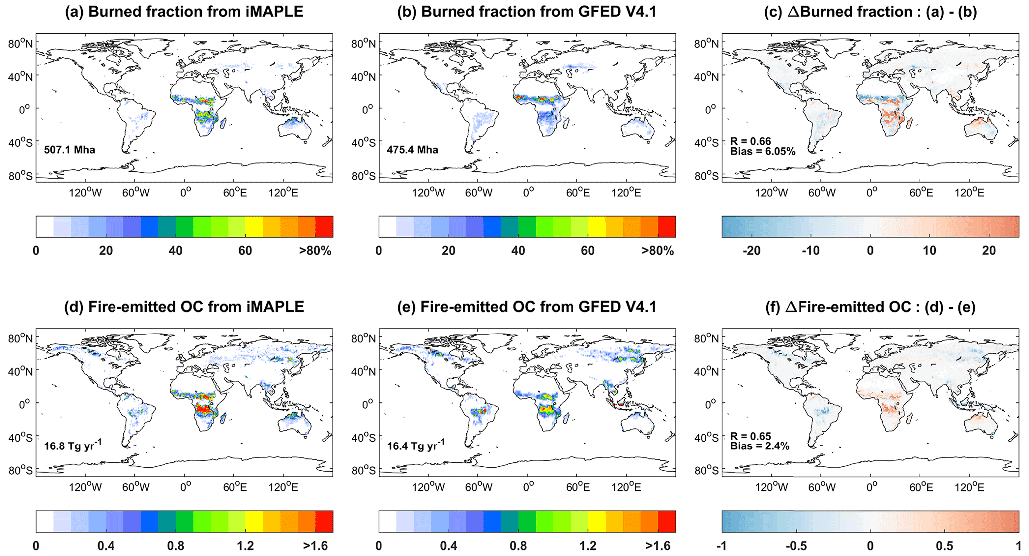
Figure 9 Comparisons of global burned fraction (%) and fire-emitted OC emissions (10⁻³ $\mathrm{kg}{\mathrm{km}}^{-\mathrm{1}}{\mathrm{yr}}^{-\mathrm{1}}$) between (a, d) simulations and (b, e) observations. Simulations are performed using iMAPLE and observations are from GFED V4.1 fire emissions products. Both simulations from the BASE experiment and observations are averaged for the 1997–2016 period. The global total area burned is shown in (a) and (b), and total OC emissions are shown in (d) and (e). The spatial difference, correlation coefficient (R), and normalized mean biases between simulations and observations are shown in (c) and (f).

The wetland emissions of CH₄ show hotspots over tropical rainforests (Fig. 10a), where the dense soil carbon provides abundant substrates for emissions and the warm climate promotes emission rates. The secondary hotspots are located in the boreal regions in the NH. This spatial pattern is very similar to the map of wetland CH₄ emissions predicted by an ensemble of 13 biogeochemical models (Saunois et al., 2020). On the global scale, the total wetland emission is 153.45 Tg [CH₄] yr⁻¹ during 2000–2014, close to the average of 148 ± 25 Tg [CH₄] yr⁻¹ for 2000–2017 estimated by multiple models. As a comparison, anthropogenic sources of CH₄ show a high amount in China and India due to the large emissions from fossil fuels and agriculture (Fig. 10b). On the global scale, the wetland emissions are equivalent to 45.3 % of the total anthropogenic emissions. As important factors driving CH₄ emissions, heterotrophic respiration shows higher values over tropical regions and eastern China with a total amount of 73.2 Pg C yr⁻¹ (Fig. 10c), and relatively high wetland coverage is found in boreal Asia and the Amazon (Fig. 10d).

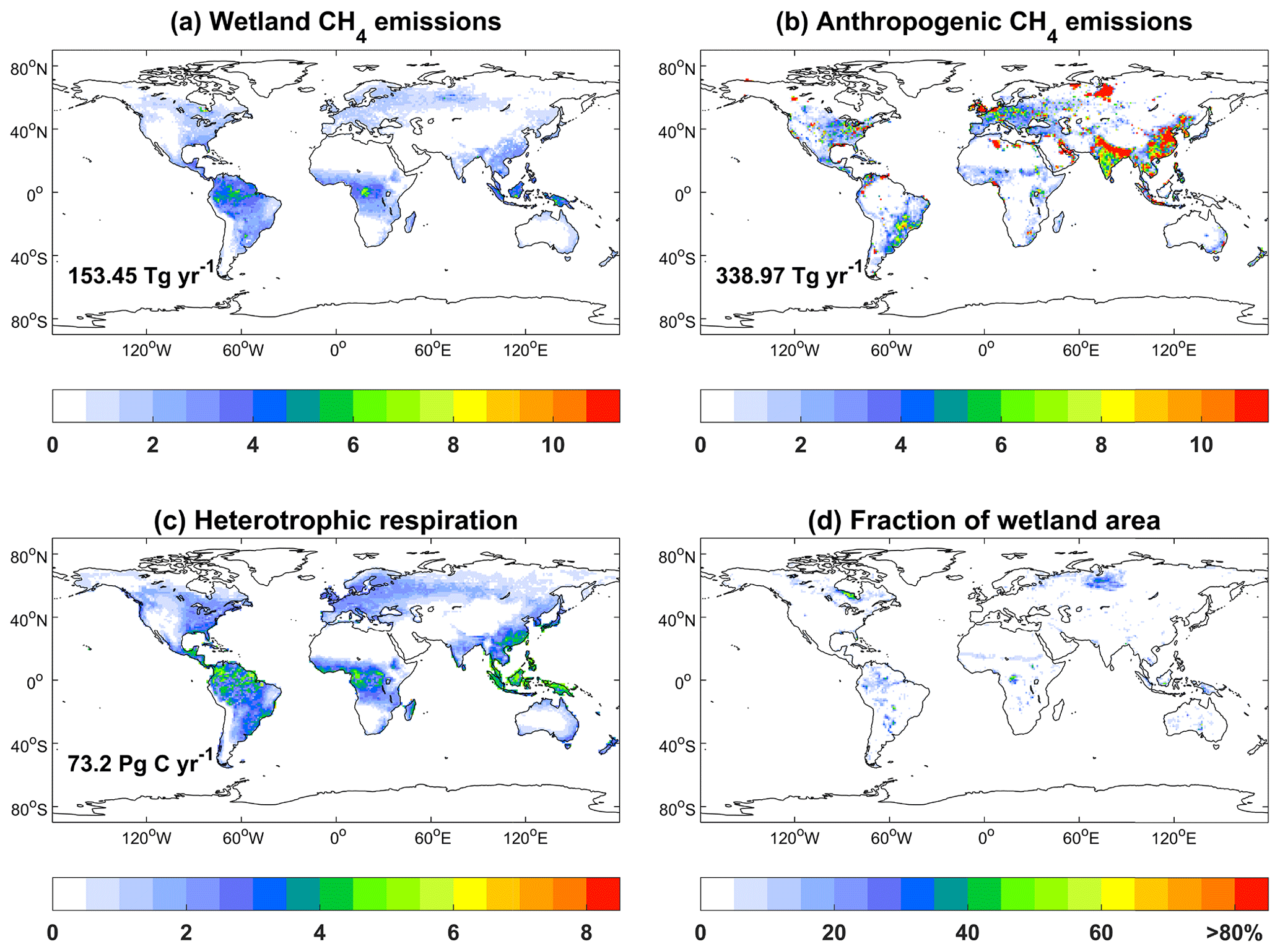
Figure 10 Global simulated CH₄ emissions ($\mathrm{g}\left[{\mathrm{CH}}_{\mathrm{4}}\right]{\mathrm{m}}^{-\mathrm{2}}{\mathrm{yr}}^{-\mathrm{1}}$) from (a) wetland and (b) anthropogenic sources, (c) heterotrophic respiration ($\mathrm{g}\mathrm{C}{\mathrm{m}}^{-\mathrm{2}}{\mathrm{d}}^{-\mathrm{1}}$), and (d) fraction of wetland area. The simulations are from the BASE experiment. Anthropogenic sources are adopted from CMIP6 including the sectors of energy, agriculture, industrial, residential, shipping, solvents, and transportation. The global total emissions and heterotrophic respirations are shown in each panel. All variables are averaged for 2000–2014.

Isoprene emissions from the two schemes in iMAPLE show similar spatial distributions with hotspots over tropical rainforest (Fig. 11), where the warm climate and abundant light are favorable for biogenic emissions. Compared to the MEGAN scheme, the PS_BVOC scheme yields higher emissions in the tropical rainforest and boreal forest but lower emissions for shrubland and grassland in semiarid regions (Fig. 11c). Such differences are attributed to the varied processes as well as the emission factors. Our earlier study showed that the PS_BVOC scheme predicts stronger trends in isoprene emissions than MEGAN (Cao et al., 2021a) because the former considers both CO₂ fertilization and inhibition effects, while the latter considers only the inhibition effects. On the global scale, isoprene emissions are 550 Tg yr⁻¹ with PS_BVOC (Fig. 11a) and 611 Tg yr⁻¹ with MEGAN (Fig. 11b). These amounts are higher than the ensemble mean of 448 Tg yr⁻¹ from the CMIP6 models (Cao et al., 2021b) but in general within the range of 412–601 Tg yr⁻¹ as summarized by Carslaw et al. (2010).

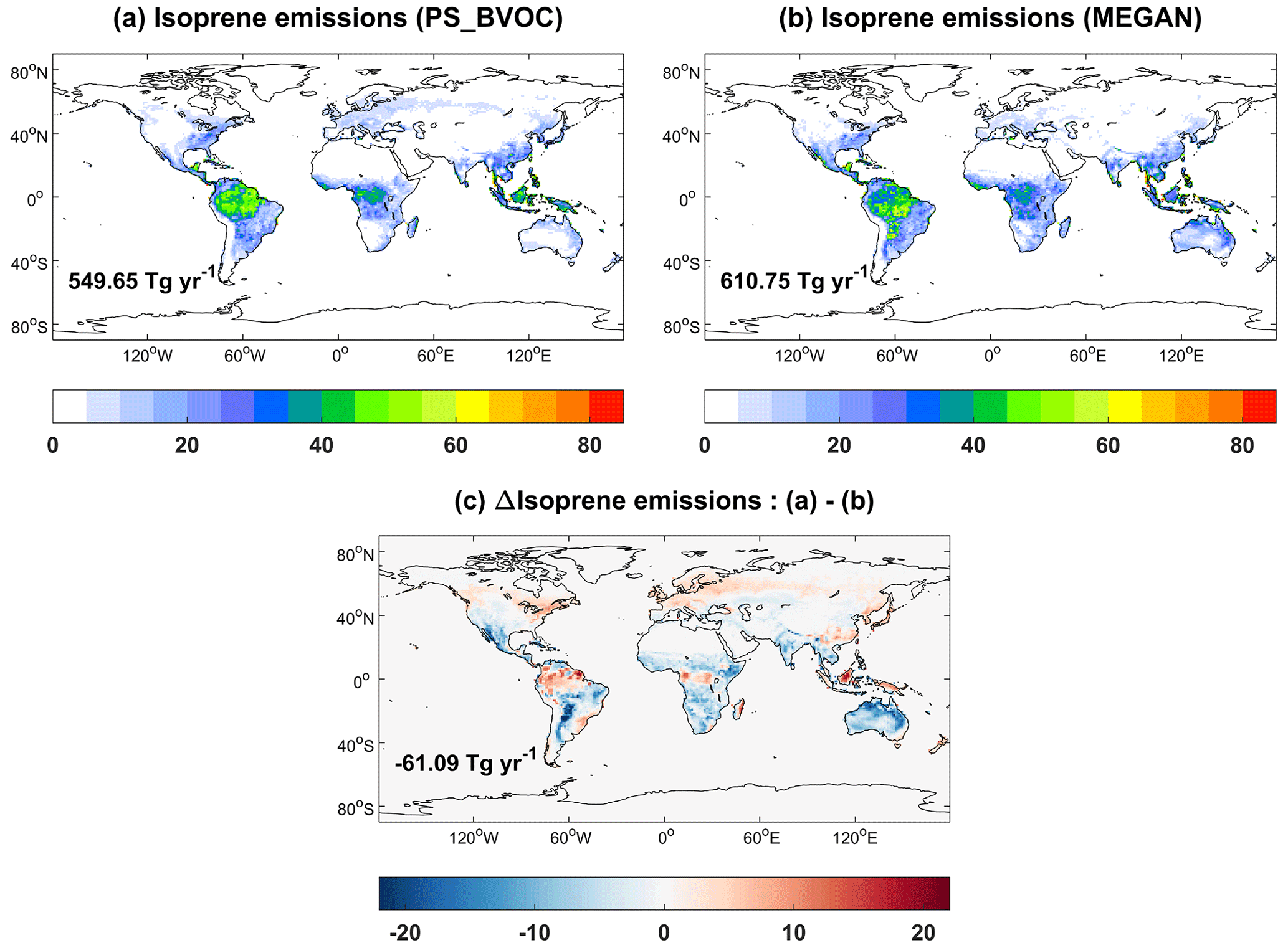
Figure 11 Global isoprene emissions ($\mathrm{mg}\mathrm{C}{\mathrm{m}}^{-\mathrm{2}}{\mathrm{d}}^{-\mathrm{1}}$) from (a) MEGAN, (b) PS_BVOC schemes, and (c) their differences during 1980–2020. The simulations are from the BASE experiment. The global total emissions are shown in each panel.

3.4 Air pollution impacts on ecosystem fluxes

We assess the damaging effects of surface O₃ on GPP with two schemes (O3LMA–BASE and O3S2007–BASE) (Fig. 12). Simulated GPP losses show similar patterns with high damage in the eastern US, western Europe, and eastern China, where the surface O₃ level is high due to anthropogenic emissions. Limited GPP damage is predicted in the tropics though with abundant forest coverage due to the low level of O₃ pollution. Compared to the S2007 scheme, predicted GPP loss is further alleviated in tropical rainforest with the LMA-based scheme because the latter scheme determines lower O₃ sensitivity for evergreen trees due to their higher content of chemical resistance with larger LMA values (Ma et al., 2023). On the global scale, the average GPP loss is −2.9 % with the LMA scheme and −3.2 % with the S2007 scheme. Such damage to GPP is weaker than the estimate of −4.8 % in Ma et al. (2023) because of the differences in O₃ concentrations, vegetation types, and photosynthetic parameters.

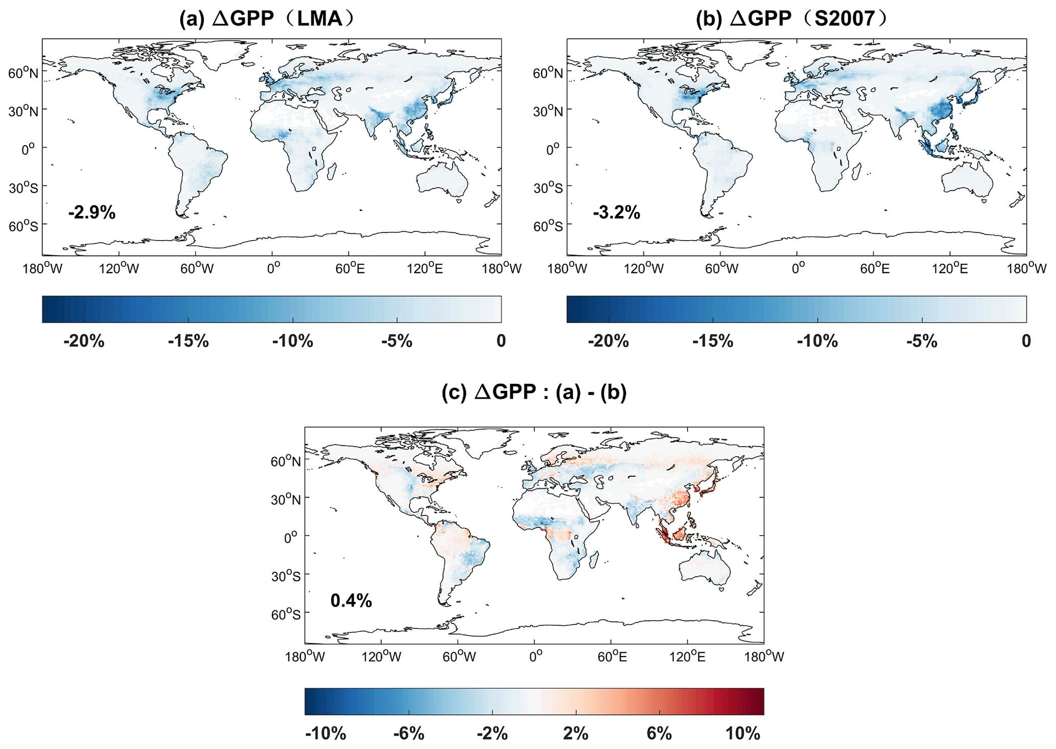
Figure 12 Percentage changes in global GPP caused by ozone damage effects based on (a) LMA (O3LMA–BASE) and (b) S2007 (O3S2007–BASE) schemes. The ozone damage schemes include (a) trait leaf mass per area (LMA) based on the O3LMA experiment, (b) S2007 plant ozone sensitivity from the O3S2007 experiment, and (c) their differences.

Atmospheric aerosols cause perturbations to both direct and diffuse radiation, which have different efficiencies in enhancing plant photosynthesis. Here, we separate the diffuse (diffuse fraction >0.75) and direct (diffuse fraction <0.25) components using the observed diffuse fraction and solar radiation at six FLUXNET sites and aggregate the GPP and ET fluxes for different radiation periods at certain intervals (Fig. 13). At the six selected sites, observed GPP is higher and grows faster with more diffusive light than that under direct light conditions (Fig. 13a–f). Simulations in general reproduce such features with the comparable variability. In the earlier study, simulated diffuse fertilization efficiency for GPP (changes of GPP per unit diffuse radiation) was well validated against observations at more than 20 sites (Yue and Unger, 2018). Such amelioration of GPP suggests that moderate aerosol loading is beneficial for ecosystem carbon uptake (Yue and Unger, 2017). However, dense aerosol loading may instead weaken plant photosynthesis due to the large reduction in direct radiation.

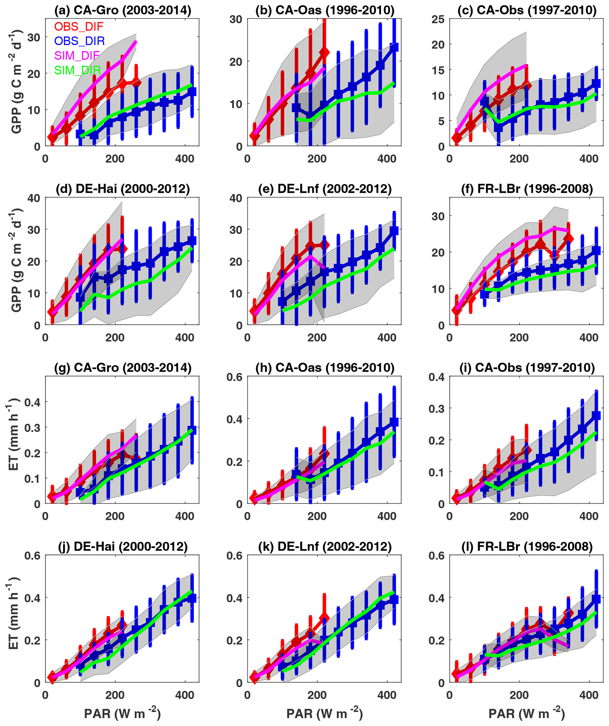
Figure 13 Observed and simulated responses of site-level (a–f) GPP and (g–l) ET to diffuse and direct radiation at the FLUXNET sites. Photosynthetically active radiation (PAR) reaching the surface is divided into diffuse (diffuse fraction >0.75) and direct (diffuse fraction <0.25) radiation at six FLUXNET sites with more than 10 years of observations. Observations (simulations) are grouped over PAR bins of 40 W m⁻² with error bars (shading) indicating standard deviations of GPP and ET for each bin. Red (blue) and magenta (green) represent observed and simulated responses of GPP and ET to diffuse (direct) radiation. Units of GPP and ET are $\mathrm{g}\mathrm{C}{\mathrm{m}}^{-\mathrm{2}}{\mathrm{d}}^{-\mathrm{1}}$ and mm h⁻¹, respectively.

We further evaluate the ET responses to diffuse and direct radiation from iMAPLE (Fig. 13g–l). Although ET is slightly higher in diffusive conditions, the growth rates are weaker than that of GPP. The main cause of such difference is related to the varied light dependence of ET components, which consist of canopy evaporation and transpiration. Transpiration is tightly coupled with photosynthesis and will increase by diffuse radiation at a similar rate. However, evaporation is more dependent on light quantity which will decrease with the extinction of aerosols. As a result, the weakened evaporation in part offsets the increased transpiration, leading to the smaller growth rate of ET than the responses of photosynthesis and the consequent enhancement in water use efficiency (Wang et al., 2023). iMAPLE reasonably captures the lower growth rates of ET than GPP in response to diffuse radiation at the selected sites.

4 Conclusions and discussion

We develop iMAPLE by coupling the Noah-MP water module with the YIBs vegetation model. Validations show that iMAPLE predicts a reasonable distribution of soil moisture and soil temperature. Driven with these prognostic soil conditions and meteorology from reanalyses, the model reasonably reproduces the observed spatiotemporal variations of both GPP and ET fluxes at 201 sites and on the global scale. We further update the biogeochemical processes in iMAPLE to extend the model's capability in quantifying interactions between air pollution and land ecosystems. The model reasonably predicts wetland CH₄ emissions at 44 sites and yields a similar global map of CH₄ emissions compared to an ensemble of 13 biogeochemical models. In addition, predicted biomass burning and biogenic emissions are consistent with either satellite retrievals or results from other models. We assess the impacts of surface O₃ and aerosols on ecosystem fluxes. The LMA-based scheme links the O₃ sensitivity with vegetation LMA and predicts a global map of GPP loss that is consistent with the traditional scheme using the PFT-specific sensitivity. The updated scheme effectively reduces modeling uncertainties by decreasing the number of parameters for O₃ sensitivity and provides an option to apply the advanced LMA map from remote sensing. The model also reproduces the observed responses of GPP and ET to diffuse radiation with a lower growth rate for ET than GPP.

There are several limitations in the current version of iMAPLE. First, it does not include the dynamic nutrient cycle. Although we implement the downregulation from Arora et al. (2009) to constrain CO₂ fertilization, this limitation is dependent only on the ambient CO₂ concentrations and could not represent the heterogeneous distribution of nutrients. As a result, the model could not reveal the biogeochemical effects of nitrogen and phosphorus deposition on land ecosystems. Second, the feedback of fire activities to ecosystems is ignored. iMAPLE considers the impacts of fuel load on area burned at each modeling time step. However, these fire perturbations do not in turn change the vegetation distribution and composition. The vegetation model does not consider the competition among PFTs so that fire perturbations are not allowed to change vegetation coverage. As a result, the interactions between fire and ecosystems are underestimated in the current model framework, potentially leading to overestimations of wildfire activity due to remaining fuel loads. Third, iMAPLE does not consider the dynamic changes in wetland area for CH₄ emissions. Although the Noah-MP module predicts runoff and underground water, the changes in hydrological cycles are not connected with wetland area in the model. Instead, a prescribed wetland dataset is applied to reduce the possible uncertainties but meanwhile limits the explorations of CH₄ changes in the historical and future periods. Meanwhile, iMAPLE considers only dynamic soil water and temperature down to the 2 m level, which may affect the interactions between climate and the land terrestrial ecosystem, especially during drier conditions. These limitations will be the focus of model development in the next step.

iMAPLE inherits the good capability of the original YIBs model in the simulations of carbon cycle. Furthermore, iMAPLE upgrades the YIBs model with carbon–water coupling and more biogeochemical processes. With iMAPLE, we could assess the changes in carbon and water fluxes, as well as their coupling, in response to environmental perturbations (e.g., climate change, air pollution, land cover change). Meanwhile, by coupling iMAPLE with climate and/or chemical models, we could further quantify the changes in meteorology and atmospheric components in response to the biogeochemical and biogeophysical processes. For example, Lei et al. (2022) revealed the strong vegetation feedback to global surface O₃ during drought periods using the YIBs model coupled to a chemical transport model. Xie et al. (2019) found a significant increase in atmospheric CO₂ concentrations due to O₃-induced vegetation damage using the YIBs model coupled with a regional climate–chemistry model. Gong et al. (2021) estimated a surface warming in polluted regions due to ozone–vegetation feedback using the YIBs model coupled with a global climate–chemistry model. These studies indicate that iMAPLE could be used either offline or online with other models to explore the interactions among climate, chemistry, and ecosystems.