Implementation and evaluation of diabatic advection in the Lagrangian transport model MPTRAC 2.6

Diabatic transport schemes with hybrid zeta coordinates, which follow isentropes in the stratosphere, are known to greatly improve Lagrangian transport calculations compared to the kinematic approach. However, some Lagrangian transport calculations with a diabatic approach, such as the Chemical Lagrangian Transport Model of the Stratosphere (CLaMS), are not well prepared to run on modern high-performance computing (HPC) architectures. Here, we implemented and evaluated a new diabatic transport scheme in the Massive-Parallel Trajectory Calculations (MPTRAC) model. While MPTRAC can be used either with shared-memory multiprocessing on CPUs or with GPUs to offload computationally intensive calculations, making it flexible for many HPC applications, it has been limited to kinematic trajectories in pressure coordinates. The extended modelling approach now enables the use of either kinematic or diabatic vertical velocities and the coupling of different MPTRAC modules based on pressure or hybrid zeta coordinates.

This study focus on the accuracy of the implementation in comparison to the CLaMS model. The evaluation of the new transport scheme in MPTRAC shows that, after 90 d of forward calculations, distributions of air parcels in the upper troposphere and lower stratosphere (UTLS) are almost identical for MPTRAC and CLaMS. No significant bias between the two Lagrangian models was found. Furthermore, after 1 d, internal uncertainties (e.g. due to interpolation or the numerical integration method) in the Lagrangian transport calculations are at least 1 order of magnitude smaller than external uncertainties (e.g. from reanalysis selection or downsampling of ERA5). Differences between trajectories using either CLaMS or MPTRAC are on the order of the combined internal uncertainties within MPTRAC. Since the largest systematic differences are caused by the reanalysis and the vertical velocity (diabatic vs. kinematic), the results support the development efforts for trajectory codes that can access the full resolution of ERA5 in combination with diabatic vertical velocities. This work is part of a larger effort to adapt Lagrangian transport in state-of-the-art models such as CLaMS and MPTRAC to current and future HPC architectures and exascale applications.

1 Introduction

The Massive-Parallel Trajectory Calculations (MPTRAC) model is a Lagrangian transport model that was developed with support for shared-memory multiprocessing on CPUs and offloading to GPUs to efficiently run on modern high-performance computing (HPC) architectures (Hoffmann et al., 2019, 2022). The MPTRAC model aims to improve upon the advection schemes of state-of-the-art Lagrangian transport models, which have, even with traditional code adaption strategies, a potentially limited capability to fully leverage the opportunities offered by recent HPC architectures (Bauer et al., 2021). One such state-of-the-art Lagrangian transport model is the Chemical Lagrangian Transport Model of the Stratosphere (CLaMS) trajectory module (McKenna et al., 2002a, b). The trajectory code of CLaMS uses only the message passing interface (MPI) to distribute air parcels across multiple processes. CLaMS is not designed for the usage of the shared-memory of compute nodes or the usage of GPUs.

However, unlike MPTRAC, CLaMS can be used with diabatic vertical velocities and a hybrid vertical coordinate (referred to as a hybrid zeta coordinate or zeta coordinate). Diabatic vertical velocities are calculated from the energy balance instead of the mass balance, as in the case of kinematic vertical velocities. The hybrid zeta coordinate was first introduced by Mahowald et al. (2002) and later implemented in CLaMS by Konopka et al. (2004). It corresponds to an orography-following sigma coordinate at the ground level and a quasi-horizontal potential temperature coordinate at levels above the ground around 380 K (Pommrich et al., 2014). This combination of hybrid zeta coordinates and diabatic velocities significantly improves Lagrangian transport simulations and trajectory calculations, especially in the stratosphere (e.g. Eluszkiewicz et al., 2000; Ploeger et al., 2010, 2011; Schoeberl and Dessler, 2011; Brinkop and Jöckel, 2019; Li et al., 2020). The improvements result from the fact that the flow in the stratosphere is mostly isentropic and that the vertical transport is closely linked to diabatic-heating rates. The implementation of the diabatic scheme is also required to couple the MPTRAC trajectory module in the future to the global three-dimensional CLaMS version including irreversible mixing (McKenna et al., 2002b; Pommrich et al., 2014; Vogel et al., 2019; Ploeger et al., 2021).

Earlier versions of MPTRAC were formulated in pressure coordinates only and were run with kinematic vertical velocities (Hoffmann et al., 2019, 2022). Following the approach of CLaMS, we implemented a new advection scheme for MPTRAC to run with diabatic vertical velocities in hybrid zeta coordinates. In addition to the approach in CLaMS, MPTRAC's advection scheme is formulated to be compatible with other modules of MPTRAC that remain in operation on pressure coordinates. Thus, in MPTRAC, advection can be performed with the diabatic scheme in zeta coordinates as in CLaMS, while, at the same time, modules based on pressure coordinates, such as the particle diffusion or convection module, can be employed (this mode is also referred to as “coupled mode” in this study). The new implementation in MPTRAC involves a role reversal between pressure and zeta coordinates and pressure and zeta tendencies. This ensures that the data structures maintain the required structure for memory sharing, multiprocessing, and offloading to GPUs. In contrast, adapting the CLaMS code for parallelization with OpenMP and OpenACC would require restructuring of loops and extensive rewriting of data structures to define proper data regions accessible to the shared memory or the GPUs.

In this study, we evaluate the accuracy of the newly implemented scheme in MPTRAC through a detailed intercomparison with results from the CLaMS model and by placing model differences in the context of the sources of uncertainty inherent in Lagrangian transport models. Uncertainty sources of Lagrangian transport models have been studied extensively in the past (e.g. Stohl, 1998; Stohl et al., 2001; Bowman et al., 2013). Uncertainty sources in transport simulations can be distinguished into external and internal sources. External uncertainties are related to the data driving the model, e.g. the reanalysis used, differences between reanalysis products, and the limited resolution of the wind data. Internal uncertainties are the necessary elements of the transport model, e.g. interpolation, integration methods, or the handling of model boundaries at the surface. To evaluate the newly implemented diabatic transport scheme in MPTRAC, we investigated the differences in trajectory calculations caused by the use of MPTRAC compared to CLaMS. To put the differences found in the trajectory calculations between CLaMS and MPTRAC in a broader context, the effects of, first, external sources (using different reanalyses at different resolutions or different vertical velocities) and, second, internal sources (e.g. interpolation and integration methods) were investigated.

External uncertainties of Lagrangian transport simulations due to differences between the used wind data are discussed frequently (e.g. Stohl et al., 2004; Angevine et al., 2014; Hoffmann et al., 2019; Li et al., 2020; Ploeger et al., 2021; Vogel et al., 2024). First of all, the limited resolution of the reanalysis fields itself creates a limitation in terms of the accuracy of the transport calculations because sub-grid-scale processes are not accounted for without parameterization (e.g. Rolph and Draxler, 1990). The stochastic parameterizations that are required to account for unresolved sub-grid-scale winds and turbulent diffusion impose an uncertainty on the transport as well. Second, reanalysis fields show systematic differences because of different dynamical cores, assimilation processes, resolutions, and parameterizations if compared with each other. Hoffmann et al. (2019) showed that systematic differences due to the chosen reanalysis (comparing ERA5 and ERA-Interim) are larger than transport deviations due to parameterized sub-grid-scale diffusion in kinematic transport calculations. Angevine et al. (2014) found, for a limited case (using FLEXPART-WRF in the troposphere), that the uncertainty in a WRF ensemble propagates into CO tracer mixing ratio uncertainties of about 30 % to 40 %. Furthermore, Stohl et al. (2004) noted that inconsistencies in reanalysis data, which are caused by separate assimilation cycles, lead to artificial diffusion in Lagrangian transport calculations. Therefore, quantities such as potential vorticity (PV) or potential temperature are less conserved than physically expected. These inconsistencies are, however, absent in forecast data and might depend on the assimilation method of a selected reanalysis. In summary, systematic differences in the reanalyses and their underlying models are expected to be a major source of external uncertainty for Lagrangian transport simulations, followed by processes that are not included in the reanalysis data (e.g. unresolved sub-grid-scale processes).

Internal uncertainties related to different integration methods applied in MPTRAC have been investigated by Rößler et al. (2018). They found that the Euler method has error growth rates that are about 1 order of magnitude higher in comparison to the mid-point scheme in the stratosphere. However, the mid-point scheme is only 2 to 4 times less accurate than third- and fourth-order Runge–Kutta schemes, with no significant differences between the third- and fourth-order schemes. Rößler et al. (2018) attribute the latter to the errors related to linear interpolation of the meteorological data, which limits the benefits of higher-order integration methods such as the fourth-order Runge–Kutta scheme. Interpolation errors, if higher-order integration is applied, could be the main internal source of error for deviations between Lagrangian transport models. Uncertainties as a consequence of interpolation have also been discussed in more detail by Stohl et al. (1995, 2001). Their results suggest interpolation and the integration scheme as the leading internal sources of uncertainty.

Differences between transport models have been studied as well. Differences in transport using different Lagrangian models (MPTRAC, CLaMS) driven by kinematic vertical velocities are smaller than differences caused by parameterized sub-grid-scale winds and turbulent diffusion (Hoffmann et al., 2019). Stohl et al. (2001) concluded, based on a comparison of three trajectory models, that the selection of the data is more important than the selection of the model for accuracy. In the literature (see also Stohl et al., 2001; Bowman et al., 2013), meteorological data are consequently considered to be the main source of uncertainty in Lagrangian transport simulations, while internal model differences, mainly due to interpolation and integration methods, are usually much smaller. Here, we validate these findings for the two most recent ECMWF reanalyses, ERA-Interim and ERA5 with CLaMS and MPTRAC.

To justify the fact that MPTRAC and CLaMS trajectory calculations can mutually substitute each other, the MPTRAC and CLaMS models do not to need to be bit-identical, but deviations must be much smaller than those from external uncertainty sources, e.g. reanalysis differences, vertical velocities, and sub-grid-scale diffusion, and must be on the order of combined internal uncertainties. In our study, we show that, after implementing hybrid zeta coordinates and diabatic vertical velocities in MPTRAC, MPTRAC, and CLaMS, results of forward-trajectory calculations differ only insignificantly. CLaMS and MPTRAC trajectory calculations can substitute each other, which bears a path forward for combined CLaMS–MPTRAC simulations in upcoming HPC systems. Further, we quantify and order in more detail the sources of transport uncertainties that are found in Lagrangian models and the driving data.

In Sect. 2 we introduce the trajectory models and the used reanalyses. Afterwards, differences between CLaMS and MPTRAC are described. Subsequently, the diagnostics used to compare the different model results and to assess the source of uncertainties are presented. In Sect. 3 the model results are evaluated, starting from case studies, going to a comparison between trajectories after 1 d, and ending with a long-term simulation of particle distributions. Finally, our conclusion is presented, that differences between CLaMS and MPTRAC trajectory calculations (as a consequence of internal sources) are negligible in comparison to the variability of the results caused by external sources such as different reanalysis or vertical velocities.

2 Methods and data

Diabatic transport calculations in hybrid zeta coordinates were implemented in MPTRAC, similarly to CLaMS. Lagrangian transport calculations rely on, first, the Lagrangian transport model itself and, second, the input wind fields that drive the model. In the following sections, the implementation of diabatic transport into MPTRAC and CLaMS, the used meteorological data, and the used diagnostic to evaluate diabatic transport in MPTRAC are described in detail.

2.1 Lagrangian transport models

CLaMS is a comprehensive chemical Lagrangian transport model including irreversible mixing and stratospheric chemistry (McKenna et al., 2002a, b; Pommrich et al., 2014; Konopka et al., 2022). Here, we focus on the advection scheme of CLaMS as a reference for the implementation of a similar advection scheme in MPTRAC. MPTRAC is a Lagrangian transport model that contains, among others, modules for advection and the parameterization of diffusion from sub-grid-scale winds and turbulence (Hoffmann et al., 2022). Trajectory calculations with both models are used in many studies, mostly focusing on UTLS and stratospheric transport processes (most recently, Liu et al., 2023; Clemens et al., 2024; Vogel et al., 2023). The implementation of diabatic transport in hybrid coordinates, i.e. of a diabatic transport scheme into MPTRAC, has four essential components: the choice of the height coordinate (hybrid zeta coordinate instead of pressure), the vertical velocity (diabatic instead of kinematic), the interpolation method, and the integration method (Runge–Kutta or mid-point). These aspects will be further discussed below.

2.1.1 Vertical coordinates

CLaMS applies the vertical hybrid zeta coordinate (ζ) with associated diabatic vertical velocity $\dot{\mathit{\zeta }}=\frac{\mathrm{d}\mathit{\zeta }}{\mathrm{d}t}$ for trajectory calculations (Mahowald et al., 2002; Konopka et al., 2004; Pommrich et al., 2014). For this study, this scheme was implemented in MPTRAC as well. The hybrid zeta coordinate is defined as shown in Eq. (1):

$$\begin{array}{}\text{(1)}& \mathit{\zeta }\left(p\right)=\left\{\begin{array}{ll}\mathit{\theta }(p,T)& \text{if}\mathit{\sigma }<{\mathit{\sigma }}_{\mathrm{r}}\\ \mathit{\theta }(p,T)\sin \left(\frac{\mathit{\pi }}{\mathrm{2}}\frac{\mathrm{1}-\mathit{\sigma }\left(p\right)}{\mathrm{1}-{\mathit{\sigma }}_{\mathrm{r}}}\right)& \text{if }\mathit{\sigma }\ge {\mathit{\sigma }}_{\mathrm{r}}\end{array}\right.,\end{array}$$

where p is the pressure, and p_s denotes the local surface pressure. $\mathit{\sigma }=\frac{p}{p_{\mathrm{s}}}$ is called the sigma coordinate, and σ_r is a reference level in the sigma coordinates. θ(p,T) is the potential temperature. Near the surface, the hybrid zeta coordinate follows the orography in the form of a sigma-like coordinate. With increasing altitude, the zeta coordinate is smoothly transformed into the potential temperature θ(p,T), which is reached at the reference level (σ_r=0.3). The reference level σ_r=0.3 corresponds to a pressure around 300 hPa (≈380 K), depending on the local surface pressure.

Equation (2) shows that the time derivative of the hybrid zeta coordinate is the time derivative of the potential temperature – the diabatic ascent rate – at altitudes above the reference level σ_r. At lower levels, the transport is a combination of diabatic rates $\dot{\mathit{\theta }}$ and kinematic rates $\dot{\mathit{\sigma }}$ (Mahowald et al., 2002; Konopka et al., 2004). The diabatic and kinematic rates are taken from reanalysis data. While the diabatic rates are derived from the energy balance including, among others, radiation, latent heat, and turbulent mixing (Ploeger et al., 2021), kinematic rates are calculated from the continuity equation.

$$\begin{array}{}\text{(2)}& \dot{\mathit{\zeta }}\left(p\right)=\left\{\begin{array}{ll}\dot{\mathit{\theta }}\left(p\right)& \text{if}\mathit{\sigma }<{\mathit{\sigma }}_{\mathrm{r}}\\ \dot{\mathit{\theta }}\left(p\right)\sin \left(\frac{\mathit{\pi }}{\mathrm{2}}\frac{\mathrm{1}-\mathit{\sigma }\left(p\right)}{\mathrm{1}-{\mathit{\sigma }}_{\mathrm{r}}}\right)\\ -\mathit{\theta }(p,T)\frac{\mathit{\pi }}{\mathrm{2}}\cos \left(\frac{\mathit{\pi }}{\mathrm{2}}\frac{\mathrm{1}-\mathit{\sigma }\left(p\right)}{\mathrm{1}-{\mathit{\sigma }}_{\mathrm{r}}}\right)\frac{\dot{\mathit{\sigma }}\left(p\right)}{\mathrm{1}-{\mathit{\sigma }}_{\mathrm{r}}}& \text{if}\mathit{\sigma }\ge {\mathit{\sigma }}_{\mathrm{r}}\end{array}\right.\end{array}$$

The diabatic approach in hybrid zeta coordinates greatly improves transport in the UTLS and stratosphere, where transport is mostly isentropic or affected by much lower diabatic-heating rates in the vertical direction. In addition, mixing often occurs quasi-horizontally on isentropic surfaces, making this coordinate ideal for application in the stratosphere.

However, the diabatic approach also has disadvantages, such as the need to smooth zeta profiles that are not monotonic with height and the fact that parameterizations developed for pressure coordinates are not accessible and would have to be reformulated. In our new implementation of diabatic vertical velocities in MPTRAC, we avoid the latter by performing the calculation of advection in zeta coordinates but transforming the zeta coordinates to pressure coordinates after advection and vice versa, from pressure to zeta coordinates before advection. In this way, other modules of MPTRAC (diffusion, convection, sedimentation, etc.) can still operate with pressure as the vertical coordinate, for which they were originally developed.

2.1.2 Numerical integration scheme

To compute Lagrangian trajectories, the ordinary differential equation $\frac{\mathrm{d}\mathit{x}\left(t\right)}{\mathrm{d}t}=\mathit{V}(t,\mathit{x})$ has to be solved. The wind field $\mathit{V}(t,\mathit{x})=(u,v,\dot{\mathit{\zeta }})$ is given on a discrete, spatio-temporal grid provided by the reanalysis. The equation is solved using the classical fourth-order Runge–Kutta method in CLaMS. In MPTRAC, both the mid-point scheme and the fourth-order Runge–Kutta method can be used (Rößler et al., 2018).

For an integration time step $t_{i+\mathrm{1}}=t_i+\mathrm{d}t$ (where dt can be lower than the temporal resolution of the data), the Runge–Kutta method is defined with the Eqs. (4) to (8).

$$\begin{array}{}\text{(3)}& {\displaystyle }{\mathit{x}}_{\mathit{i}\mathbf{+}\mathbf{1}}={\mathit{x}}_{\mathit{i}}+{\displaystyle \frac{\mathrm{1}}{\mathrm{6}}}\left({\mathit{k}}_{\mathbf{1}}+\mathrm{2}{\mathit{k}}_{\mathbf{2}}+\mathrm{2}{\mathit{k}}_{\mathbf{3}}+{\mathit{k}}_{\mathbf{4}}\right)\mathrm{d}t\text{(4)}& {\displaystyle }\text{(5)}& {\displaystyle }{\mathit{k}}_{\mathbf{1}}=\mathit{V}(t_i,x_i)\text{(6)}& {\displaystyle }{\mathit{k}}_{\mathbf{2}}=\mathit{V}\left(t_i+{\displaystyle \frac{\mathrm{d}t}{\mathrm{2}}},{\mathit{x}}_{\mathit{i}}+\mathrm{d}t{\displaystyle \frac{{\mathit{k}}_{\mathbf{1}}}{\mathrm{2}}}\right)\text{(7)}& {\displaystyle }{\mathit{k}}_{\mathbf{3}}=\mathit{V}\left(t_i+{\displaystyle \frac{\mathrm{d}t}{\mathrm{2}}},{\mathit{x}}_{\mathit{i}}+\mathrm{d}t{\displaystyle \frac{{\mathit{k}}_{\mathbf{2}}}{\mathrm{2}}}\right)\text{(8)}& {\displaystyle }{\mathit{k}}_{\mathbf{4}}=\mathit{V}\left(t_i+\mathrm{d}t,{\mathit{x}}_{\mathit{i}}+\mathrm{d}t{\mathit{k}}_{\mathbf{3}}\right)\end{array}$$

The mid-point scheme, which is a second-order Runge–Kutta scheme, is defined by Eq. (9).

$$\begin{array}{}\text{(9)}& {\mathit{x}}_{i+\mathrm{1}}={\mathit{x}}_i+\mathrm{d}t\mathit{V}\left(t_i+{\displaystyle \frac{\mathrm{d}t}{\mathrm{2}}},{\mathit{x}}_{\mathit{i}}+{\displaystyle \frac{\mathrm{d}t}{\mathrm{2}}}\mathit{V}(t_i,{\mathit{x}}_i)\right)\end{array}$$

While the Runge–Kutta method has a fifth-order truncation error (𝒪(dt⁵)) and a fourth-order accumulated error (𝒪(dt⁴)), the mid-point scheme has a third-order (𝒪(dt³)) truncation error and a second-order accumulated error (𝒪(dt²)) (Rößler et al., 2018).

2.1.3 Interpolation

For the integration of the diabatic transport scheme into MPTRAC, MPTRAC was equipped with functions to read the vertical velocities of the hybrid zeta coordinate ($\dot{\mathit{\zeta }}$) from files that follow the data structure of CLaMS. Moreover, during the integration time steps, the horizontal wind and vertical velocity must be interpolated to the air parcel locations. Therefore, a new interpolation function for MPTRAC was implemented.

For the Runge–Kutta method, wind fields must be interpolated four times to the given time, horizontal location, and zeta height. For the mid-point scheme, this is reduced to two interpolations. For MPTRAC and CLaMS, four-dimensional linear interpolation methods are performed, which are common for Lagrangian transport models (Bowman et al., 2013). However, the specific details of the interpolation in CLaMS and MPTRAC differ because the wind fields are not regularly provided in hybrid zeta coordinates but rather in hybrid eta coordinates, as applied in ECMWF's Integrated Forecasting System (Simmons et al., 1989). Interpolation with positions given only in zeta coordinates therefore requires additional considerations, e.g. about how to find the vertical position of the box that includes an air parcel, when the data are not stored in the air parcel coordinate. In addition, MPTRAC has modules that rely on a formulation in pressure coordinates, requiring frequent conversions of the air parcel position from pressure to zeta and vice versa. For example, the air parcel position given in the zeta coordinate is updated during the advection time step. Afterwards, the updated position in zeta coordinates is converted to pressure. The air parcel position given in pressure coordinates can then be updated by using a module such as for turbulent diffusion, which adds a random increment to the air parcel position in pressure coordinates. Afterwards, the air parcel position in pressure needs to be transformed back to the zeta coordinates again for use with the diabatic advection. Therefore, the performed interpolations are required to be precisely invertible. A further difference is that time interpolation is performed locally for each air parcel in MPTRAC, e.g. wind data are collected around the position of the air parcel and subsequently interpolated in time. In contrast, CLaMS interpolates the wind field in time and globally in advance for the four time steps of the Runge–Kutta scheme, i.e. the entire wind data field is interpolated in time and subsequently used for all air parcels.

As a consequence of the mentioned differences between the models, the interpolations of CLaMS and MPTRAC follow two different concepts. Figure 1 illustrates the two concepts in two-dimensional space (height vs. longitude) in a simplified case. Two neighbouring vertical profiles of pressure and zeta are selected in eta coordinates. The goal is to interpolate from zeta to pressure and back to zeta. For simplicity, it is assumed that each eta level has constant pressure levels. Then, in CLaMS, the interpolation begins with a vertical interpolation along the two profiles. For this step, the vertical position of the air parcel is identified along each vertical profile separately using the height of the air parcel in zeta (ζ_AP). As a consequence, the pressure data (p_AP,1, p_AP,2) of two different eta levels are collected for final horizontal interpolation, provided that the zeta profiles vary strongly enough from location to location. With the final horizontal linear interpolation, the pressure at the air parcel position is given. However, if this pressure position is used to interpolate back to the zeta coordinate again, which is required for MPTRAC, the identified vertical location from the pressure height might differ from the vertical position in zeta height. To illustrate this issue, Fig. 1a describes the case where pressure levels agree with the eta levels. Hence, with one single pressure provided as the air parcel position, only one box – the box with index i, where $p_{i+\mathrm{1}}\le p_{\mathrm{AP}}<p_i$ – will be selected for the interpolation back to zeta. Since the data used for the interpolation from zeta to pressure (data from multiple eta levels) do not agree with the data used for the interpolation from pressure to zeta (data from one eta level), the interpolation is not reversed accurately.

To overcome this issue, MPTRAC instead starts with the horizontal interpolation of the zeta values and pressure values according to the horizontal air parcel position (λ_AP) at every eta level. This is depicted as simplified in Fig. 1b. The procedure provides a vertical profile of pressure (p_i) and zeta (ζ_i) centred at the horizontal position of the air parcel. Along this profile, the unique box that contains the air parcel in both coordinates can be found. This profile can then also be reversed exactly by linear vertical interpolation. To avoid interpolation of zeta and pressure at all eta levels, the right height index is found by an iterative method. The exact interpolation of both models is described in the following paragraphs.

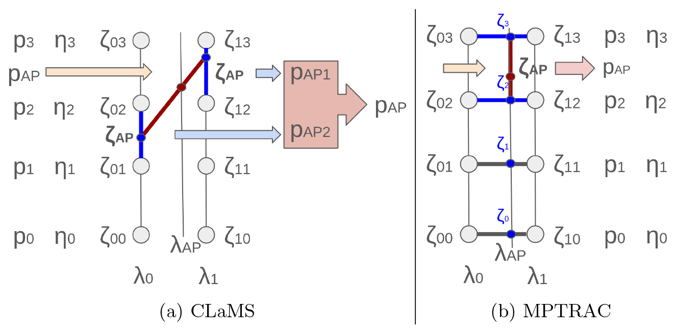
Figure 1 Concept of the interpolation illustrated in two dimensions for (a) CLaMS and (b) MPTRAC. Small circles indicate grid points, where the zeta and pressure values are given. Blue lines indicate the direction of the first interpolation, and red lines indicate the direction of the second interpolation.

Figure 2 illustrates the interpolation as implemented in CLaMS (also referred to as interpolation “V0” in this study). Let ζ_ijkl be the zeta coordinate and Q_ijkl a quantity which is supposed to be interpolated to the position of the air parcel. Both the coordinate and the quantity are required to be formulated in a hybrid eta coordinate. In detail, the indices $i,j,k$ refer to the indices on the three-dimensional grid in longitude λ_i, latitude ϕ_j, and the vertical hybrid eta coordinate η_k. The index l refers to the time t_l. Furthermore, let $({\mathit{\lambda }}_{\mathrm{AP}},{\mathit{\varphi }}_{\mathrm{AP}},{\mathit{\zeta }}_{\mathrm{AP}},t_{\mathrm{AP}})$ be the position and time of the air parcel to which the quantity Q_ijkl needs to be interpolated. In CLaMS, at first, the interpolation in time is performed. For this purpose, the neighbouring times t₀ and t₁ are selected so that $t_{\mathrm{0}}\le t_{\mathrm{AP}}<t_{\mathrm{1}}$ (see Fig. 2 (1)). With the data from the neighbouring times, a linear interpolation of ζ_ijkl and Q_ijkl is done to the time t_AP (see Fig. 2 (2)). This provides three-dimensional fields of ζ_ijk and Q_ijk (see Fig. 2 (3)). Then, the horizontal indices of the air parcel are determined (i_AP,j_AP) using the horizontal coordinates λ_AP and ϕ_AP and the horizontal grid of longitudes λ_i and latitudes ϕ_j (see Fig. 2 (4)). The indices define a column which includes the air parcel (see Fig. 2 (5)). Subsequently, within this column, four vertical indices are determined by locating the indices $(k_{i_{\mathrm{AP}},j_{\mathrm{AP}}},k_{i_{\mathrm{AP}}+\mathrm{1},j_{\mathrm{AP}}},k_{i_{\mathrm{AP}},j_{\mathrm{AP}}+\mathrm{1}},k_{i_{\mathrm{AP}}+\mathrm{1},j_{\mathrm{AP}}+\mathrm{1}})$ with ${\mathit{\zeta }}_{k_{i_{\mathrm{AP}},j_{\mathrm{AP}}}}\le {\mathit{\zeta }}_{\mathrm{AP}}<{\mathit{\zeta }}_{k_{i_{\mathrm{AP}},j_{\mathrm{AP}}}+\mathrm{1}}$, etc., along the four edges of the column (see Fig. 2 (6)). Then, at these four vertical indices and the indices one level higher, the values of ζ_ijk and Q_ijk are collected to define a box for the interpolation (see Fig. 2 (7)). In this box, the quantity Q_ijk is first interpolated vertically four times to the respective ζ_AP (see Fig. 2 (8)). Now, the quantity Q_ijkl is given on the four corners of the plane with ζ=ζ_AP (see Fig. 2 (9)). Finally, the quantity is interpolated horizontally, taking into account the line elements of the spherical coordinates (see Fig. 2 (10)). This provides $Q({\mathit{\lambda }}_{\mathrm{AP}},{\mathit{\varphi }}_{\mathrm{AP}},{\mathit{\zeta }}_{\mathrm{AP}},t_{\mathrm{AP}})$.

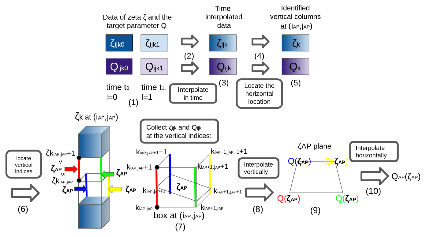
Figure 2 Schematic steps during interpolation V0 of a quantity Q to the air parcel position in zeta coordinates in CLaMS. For further details, see the text.

The interpolation from pressure to zeta and from zeta to pressure is particularly important when coupling geophysical modules that operate with pressure as the vertical coordinate (e.g. convection, diffusion, and sedimentation), as is the case for MPTRAC. The precise and accurate inversion of the interpolation in CLaMS from pressure back to zeta coordinates is difficult because, during step (6), height indices can be found from the pressure that are inconsistent with height indices found using the zeta coordinate positions. Then, significant errors may occur, making this approach unsuitable for frequent transformations between zeta and pressure coordinates. Consequently, a fully reversible interpolation algorithm has been developed for MPTRAC to allow the coupling of pressure-based modules with the diabatic advection scheme, where frequent vertical coordinate inversions are required.

Figure 3 shows a schematic of the interpolation in MPTRAC (which is also referred to as interpolation “V2”, while it is referred to as the original interpolation of MPTRAC with “V1”). With the same definitions as for the interpolation of CLaMS, the interpolation in MPTRAC can be described as follows. The interpolation also starts by selecting the data of ζ_ijkl and Q_ijkl for the neighbouring times, i.e. t₀ and t₁ (see Fig. 3 (1)). Then, the horizontal indices of the air parcel are determined (i_AP,j_AP) (see Fig. 3 (2)). The indices define two columns which include the air parcel at the times t₀ and t₁ (see Fig. 3 (3)). Consequently, for each of these columns, four vertical indices are determined by locating the indices $(k_{i,j},k_{i+\mathrm{1},j},k_{i,j+\mathrm{1}},k_{i+\mathrm{1},j+\mathrm{1}}{)}_{t_{\mathrm{0}}}$ and $(k_{i,j},k_{i+\mathrm{1},j},k_{i,j+\mathrm{1}},k_{i+\mathrm{1},j+\mathrm{1}}{)}_{t_{\mathrm{1}}}$ along the eight edges of the two columns, analogously to the procedure in CLaMS (see Fig. 3 (4)). However, afterwards, the minimum and maximum indices k_min and k_max among the vertical indices from both times are determined (see Fig. 3 (5)). The minimum index and maximum index define the start and end points of an iteration that locates the box that contains the air parcel in the vertical direction. The iteration starts with the temporal and horizontal interpolation of ζ_ijkl at the bottom and top of a box, which is defined by the minimum vertical index k_min and the spatial indices (i_AP,j_AP) (see Fig. 3 (6) and (7)). After the interpolation, ζ is given at the top ζ_top and the bottom ζ_bottom of the box (see Fig. 3 (8)). If ζ_AP is lower than ζ_top and equal to or higher than ζ_bottom, the iteration finishes. Otherwise, the iteration proceeds by going to the next higher index until the right box is found. Because of the strictly monotonic increase in ζ_ijkl with height, it is guaranteed that the right box is found between the minimum and maximum vertical indices. However, when the right box is found, the quantity Q_ijkl is also interpolated temporally and horizontally to the top Q_top and Q_bottom of the correct box (see Fig. 3 (9)), analogously to the interpolation of ζ_ijkl in (6) and (7). Finally, the vertical interpolation is performed linearly by using the quantity Q_ijkl and the coordinate ζ_ijkl from the top and bottom of the box and the zeta coordinate (ζ_AP) of the air parcel (see Fig. 3 (9)). This provides $Q({\mathit{\lambda }}_{\mathrm{AP}},{\mathit{\varphi }}_{\mathrm{AP}},{\mathit{\zeta }}_{\mathrm{AP}},t_{\mathrm{AP}})$. If Q_ijkl is a vertical coordinate, such as pressure, the interpolation can be reversed as the vertical indices in Q_ijkl can also be determined in step (4) of Fig. 3 from the respective vertical Q_ijkl profiles.

The algorithm in MPTRAC allows precise interpolation from zeta to pressure and back to zeta because the vertical column at the horizontal position of the air parcel gives a monotone relationship between zeta and pressure. In particular, the processing of pressure and zeta is analogous with opposite roles. The vertical 1D linear interpolation at the final step (9) can be performed accurately and unambiguously.

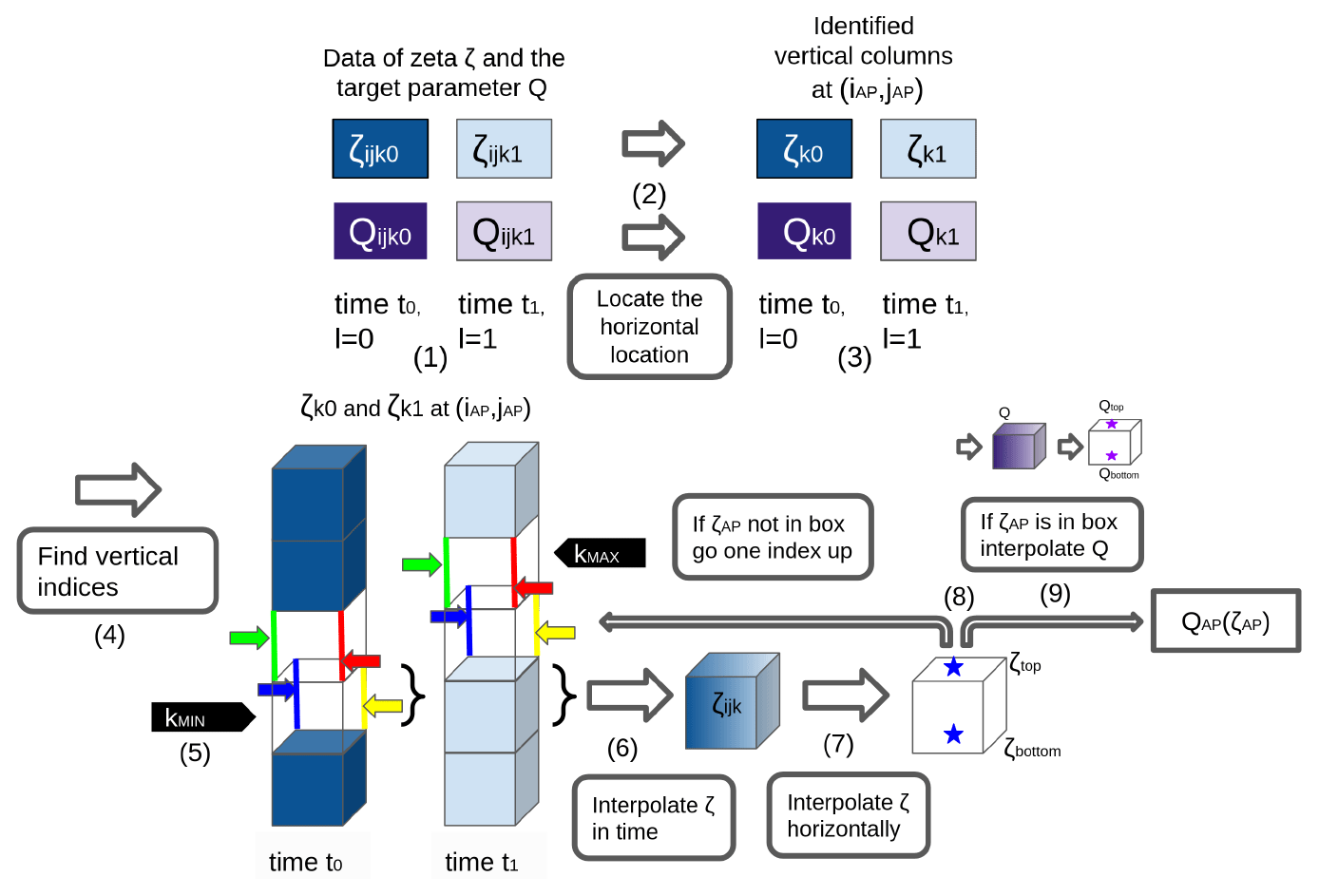
Figure 3 Schematic steps during interpolation V2 of a quantity Q to the air parcel position in zeta coordinates in MPTRAC. For further details, see the text.

For comparison and error estimations, a third interpolation variant was implemented into MPTRAC, resembling more closely the interpolation in CLaMS (called interpolation “V3”). In this approach, the interpolation procedure follows the first steps (1) to (5) as defined in V2 and Fig. 3. Afterwards, however, the two profiles given in step (5) are combined to interpolate in time along the four edges between k_min and k_max so that the location of the vertical indices and the interpolation on a zeta plane can finally be done, as for CLaMS (see Fig. 2, steps (6) to (10)).

However, note that all interpolations in MPTRAC are performed in Cartesian coordinates. That is, the line elements of the spherical-coordinate system are not applied to the air parcel positions during interpolation – rather, this is done so afterwards, assuming that the differences in the line elements within a grid box are negligible. The transformation from Cartesian coordinates to spherical coordinates is done separately from the interpolation process by applying the equations $\mathrm{\Delta }\mathit{\lambda }=\frac{\mathrm{\Delta }x}{R_{\mathrm{E}}\cos \mathit{\varphi }}$ and $\mathrm{\Delta }\mathit{\varphi }=\frac{\mathrm{\Delta }y}{R_{\mathrm{E}}}$. Δx and Δy denote the changes in Cartesian coordinates, Δϕ and Δλ denote the change in spherical coordinates, and R_E denotes the Earth radius. These transformations are not applied in CLaMS because interpolation is already done in spherical coordinates.

Finally, pressure is interpolated logarithmically in CLaMS for zeta levels higher than 1000 K and linearly for levels below 500 K. In between those levels, the linear and logarithmic interpolations are combined. In contrast, MPTRAC uses linear interpolation for pressure on all hybrid zeta levels.

2.1.4 Further model differences

MPTRAC uses spherical coordinates to store the position of air parcels. CLaMS has a hybrid approach, with spherical coordinates for air parcels at latitudes between −72° S and 72° N, but otherwise uses a stereographic projection at high latitudes (McKenna et al., 2002b). The approach in CLaMS guarantees that the integration does not diverge near the poles.

In MPTRAC the spherical-coordinate singularity is handled differently. In MPTRAC, for air parcels very close to the pole (i.e. closer than 110 m or 0.001° latitude), the zonal transport is ignored. Horizontal coordinates are calculated with double precision to guarantee the required accuracy for this approach. The method has been shown to be reliable for different applications (e.g. Hoffmann et al., 2017; Rößler et al., 2018).

Both models use the shallow-atmosphere approximation. This means that the horizontal plane is transformed from spherical to Cartesian coordinates, assuming that the height of the air parcel is negligible with respect to the Earth's radius. The two models have slight differences in the Earth's radius. In MPTRAC's default setting, the Earth's radius is assumed to be 6367.421 km, whereas in CLaMS, it is 6371.000 km. This has implications for transformations between the Cartesian and spherical-coordinate systems.

2.2 Reanalysis data

The full-resolution ERA5, downsampled ERA5, and ERA-Interim reanalyses were used to run the forward trajectory calculations with CLaMS and MPTRAC. ERA5 and ERA-Interim are provided by the ECMWF (Dee et al., 2011; Hersbach et al., 2020). ERA5 is the successor of ERA-Interim; 6-hourly meteorological data at about 80 km horizontal resolution on 60 levels are provided by the ERA-Interim reanalysis. The levels start at the surface, and the upper limit of the reanalysis is at 0.1 hPa. The ERA-Interim reanalysis covers the years from 1979 to 2019. A four-dimensional variational analysis (4D-Var) with a 12 h time window, in combination with the ECMWF's Integrated Forecast System (IFS) cycle 31r2, is used for the assimilation of meteorological observations in ERA-Interim.

The ERA5 reanalysis provides hourly meteorological data with 30 km horizontal grid resolution (sampled at 0.3° × 0.3°). ERA5 has 137 levels from the surface up to 80 km. In contrast to the ERA-Interim reanalysis, the ERA5 reanalysis was created with the IFS cycle 41r2 and hence benefits from model improvements, such as new parameterizations of atmospheric waves and convection. The assimilation in ERA5 is performed with four-dimensional variational analysis as well. The ERA5 reanalysis provides data for the years between 1950 and the present. It was shown that the ERA5 reanalysis significantly improves Lagrangian transport simulations in the free troposphere and stratosphere and has considerable differences compared to ERA-Interim (Hoffmann et al., 2019).

The downsampled version of ERA5 (referred to as ERA5 1° × 1°) was computed, applying a truncation to T213 using the ECMWF MARS data processing system. The downsampled version has 1° × 1° horizontal sampling and 6 h temporal sampling. However, ERA5 1° × 1° has the same vertical resolution as ERA5. ERA5 1° × 1° is used in transport calculations to profit from the enhancements of the ERA5 reanalysis on the one hand but to reduce computing time and difficulties handling large data sets, such as full-resolution ERA5, on the other hand (e.g. Ploeger et al., 2021).

2.3 Diagnostics to evaluate the diabatic transport in MPTRAC

2.3.1 Model runs

The implementation of the diabatic transport scheme in MPTRAC, used with the ERA5 reanalysis, is evaluated by a detailed intercomparison with CLaMS trajectory calculations for a global ensemble of air parcels. To put the differences found in the trajectory calculations between CLaMS and MPTRAC in a broader context, the effects of, first, external sources (using different reanalyses, resolutions, and vertical velocities) and, second, internal sources (e.g. interpolation and integration methods) were investigated. For the evaluation of the newly implemented diabatic scheme in MPTRAC, we use a model initialization with about 1.4 million globally distributed trajectory seeds. The forward calculations are calculated for the boreal summer (June, July, August). Short-term calculations of 1 d are initialized on 1 July 2016, while the long-term calculations of 90 d are started on 1 June 2016 to cover the entire boreal summer and austral winter. Seasonal differences are taken into account by separately analysing the Northern Hemisphere and the Southern Hemisphere. The air parcels are distributed horizontally quasi-homogeneously so that they have an average mutual distance of about 100 km. Vertically, they are distributed in specific layers. The layers are constructed such that each air parcel represents the same amount of entropy in the atmosphere, which is a product of density and the logarithm of the potential temperature (Konopka et al., 2007). For this reason, most air parcels are initialized around the tropopause, where the entropy of the atmosphere is largest. However, the air parcels cover a total zeta range from 30 K (about 1 km) to about 2000 K (about 48 km). Setups similar to the one used here are often used to initialize transport calculations with CLaMS for studies in the UTLS and, in particular, are constructed to fit the hybrid zeta coordinates and mixing concept in CLaMS (e.g. Konopka et al., 2007; Pommrich et al., 2014; Vogel et al., 2015, 2019; Konopka et al., 2007). Additionally, air parcels that reach the lower model boundary (ζ=0) are terminated in CLaMS. For comparison only, the same concept was applied in MPTRAC, too.

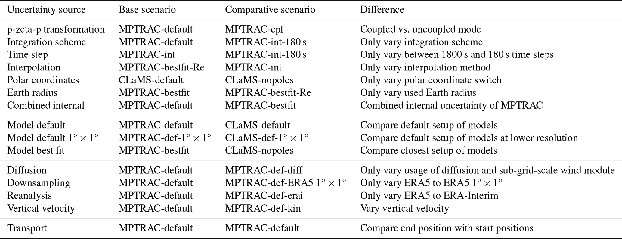
We employ different simulation scenarios to put the deviations of the two models into the perspective of known uncertainty sources. Table 1 presents the scenarios where different components of the transport calculations, such as the interpolation, integration, earth radius, coordinate systems, reanalysis, resolution, diffusion parameterization, and the vertical velocity, are varied. By comparing these scenarios, we can estimate uncertainties from different sources. Table 2 summarizes the different scenario intercomparisons and the related exposed uncertainty sources.

Table 1 Overview of different simulation scenarios for transport calculations with MPTRAC and CLaMS.

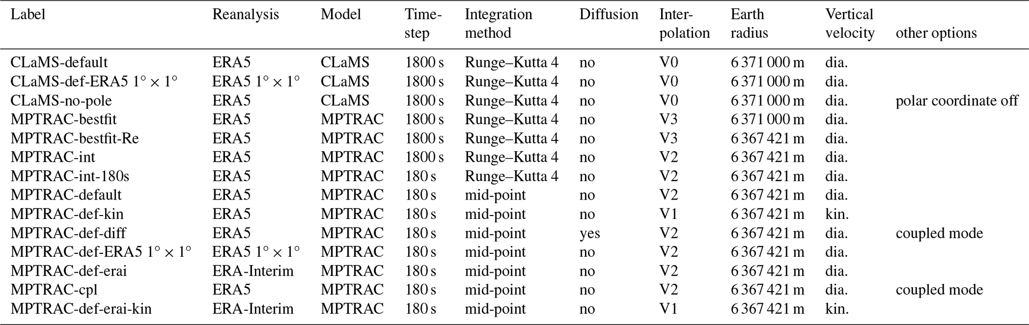
Table 2 Scenario intercomparisons for the estimation of different uncertainties in the Lagrangian transport calculations. Two scenarios are compared (base and comparative scenario) for the estimation. In most cases, only one aspect of the model setup is varied. The first block focuses on internal uncertainties of CLaMS and MPTRAC separately. The second block focuses on the comparison of the two models. The third block focuses on the external uncertainties. The last block describes the “transport”, i.e. the difference between the start and the end point of a trajectory. Transport is not an uncertainty source, but it is a useful quantity for intercomparison with the uncertainties.

The sources of uncertainty are classified into internal, model, and external uncertainties. The first block of uncertainties in Table 2 describes the internal uncertainties. Internal sources for model uncertainties are based on the model code of a Lagrangian transport model itself, such as the vertical coordinate transformation from pressure to zeta or the integration scheme. These uncertainties are not estimated by comparing two different models but by comparing two different configurations of the same model and hence give an indication of the order of magnitude of the uncertainty already present within a model. A combination of all internal uncertainty sources within MPTRAC (see labels “interpolation”, “integration scheme”, “earth radius”, and “time step”) is also investigated (see label “combined internal uncertainty”).

Model differences (“model default”, “model default 1° × 1°”, and “model best fit”) are the combination of uncertainties between two models and are listed in the second block of Table 2. Often, the sources that cause the model uncertainties are not known. The model uncertainties can be caused by the estimated internal uncertainties if the models also differ in the methods used. However, additional sources of uncertainties are possible. For example, the interpolation methods between MPTRAC and CLaMS vary more than can be estimated from the variation of the interpolation methods implemented in MPTRAC. While the interpolation in MPTRAC is always in Cartesian coordinates, CLaMS uses spherical coordinates.

External uncertainties are used to show the significance of calculations with the fully resolved ERA5 and diabatic vertical velocities. Therefore, different reanalysis products such as ERA5, ERA-Interim, and ERA5 1° × 1° are compared. In addition, the vertical velocity approach and the uncertainty from unresolved sub-grid-scale winds are investigated in the scenarios.

Finally, we introduce the deviation between the initial position of the air parcels and their final position as a physical reference to compare with. This deviation is labelled “transport” in Table 2. Transport is not an uncertainty source, but it is a useful quantity for intercomparison with the uncertainties.

2.3.2 Diagnostics for model uncertainties and differences

For the intercomparison of the different model scenarios, a set of frequently used diagnostics was applied (e.g. Stohl et al., 1995; Hoffmann et al., 2019). Let i and j denote the indices of two trajectories with the same initial position derived in two different scenarios, and let t denote the time at which the comparison is done. Then the air-parcel-wise absolute vertical transport deviation (AVTD) at a given time t in the vertical zeta coordinate is

$$\begin{array}{}\text{(10)}& {\mathrm{AVTD}}_{\mathit{\zeta }}=\left|{\mathit{\zeta }}_i\right(t)-{\mathit{\zeta }}_j(t\left)\right|.\end{array}$$

The absolute deviation in the vertical direction quantifies the differences between individual air parcels. If kinematic calculations are compared with diabatic calculations, the zeta coordinates are calculated from temperature, surface pressure, and the air parcels pressure according to Eq. (1) for both calculations. Otherwise, the zeta coordinate is directly given.

The log-pressure altitude is defined as $Z=H\log \frac{p_{\mathrm{0}}}{p}$, where p₀=1013.25 hPa and H=7.0 km. Then, the air-parcel-wise AVTD in log-pressure altitude is

$$\begin{array}{}\text{(11)}& {\mathrm{AVTD}}_Z=\left|Z_i\right(t)-Z_j(t\left)\right|.\end{array}$$

To calculate the air-parcel-wise absolute horizontal transport deviation (AHTD), the equation we use is

$$\begin{array}{}\text{(12)}& \mathrm{AHTD}=\sqrt{\left(x_i\right(t)-x_j(t){)}^{\mathrm{2}}+(y_i\left(t\right)-y_j\left(t\right){)}^{\mathrm{2}}+\left(z_i\right(t)-z_j(t){)}^{\mathrm{2}}},\end{array}$$

where $(x_i,y_i,z_i)$ and $(x_j,y_j,z_j)$ are the positions of the air parcels in Cartesian coordinates. The Euclidean distance approximates the great-circle distance for distances up to 5000 km with high precision (Hoffmann et al., 2019). For larger deviations, i.e. in calculations longer than 1 d, the great-circle distance itself is used as the air-parcel-wise AHTD:

$$\begin{array}{}\text{(13)}& \mathrm{AHTD}=R_{\mathrm{E}}\arccos \left(\sin {\mathit{\varphi }}_{\mathrm{1}}\sin {\mathit{\varphi }}_{\mathrm{2}}+\cos {\mathit{\varphi }}_{\mathrm{1}}\cos {\mathit{\varphi }}_{\mathrm{2}}\cos |{\mathit{\lambda }}_{\mathrm{1}}-{\mathit{\lambda }}_{\mathrm{2}}|\right),\end{array}$$

where ϕ_i and ϕ_j are the latitudes of the air parcels, and λ_i and λ_j are the longitudes of the air parcels. R_E is the Earth radius.

To measure the conservation error of a quantity q such as potential temperature at time t, the air-parcel-wise relative tracer conservation error (RTCE) is used:

$$\begin{array}{}\text{(14)}& \mathrm{RTCE}=\mathrm{2}{\displaystyle \frac{\mid q\left(t\right)-q\left(\mathrm{0}\right)\mid }{\mid q\left(t\right)\mid +\mid q\left(\mathrm{0}\right)\mid }}.\end{array}$$

Individual trajectories of air parcels can substantially deviate between the scenarios defined in Table 1. Statistics such as quantiles, means, and medians of the different air-parcel-wise diagnostics for about 1.4 million air parcels are considered to robustly quantify deviations independently from single air parcel outcomes. Note that Stohl et al. (1995) and Hoffmann et al. (2019) define the absolute trajectory deviations and conservation errors as the average over the above air-parcel-wise absolute trajectory deviations. Here, in contrast, it is referred to as the air-parcel-wise diagnostics with AVTD, AHTD, and RTCE. The statistical moments and quantiles are explicitly mentioned (e.g. mean AVTD for the average over all air-parcel-wise AVTDs).

3 Results

3.1 Examples of trajectories and transport deviations

The simulations are initialized globally and cover almost the entire height range of the free troposphere and stratosphere (about 1–50 km), allowing for the analysis of numerous meteorological conditions and different trajectories. Figure 4 shows exemplary trajectories for a duration of 10 d, highlighting transport in the troposphere, quasi-horizontal transport in the upper troposphere and lower stratosphere (UTLS), and fast transport in the lower stratosphere (LS).

The model deviations are significantly smaller than deviations from external sources such as downsampling of reanalysis data, different vertical velocities, variations in reanalysis data sets (here from ERA5 to ERA-Interim), or the influence of atmospheric diffusion. Trajectories with ERA5 1° × 1° roughly follow the fully resolved ERA5 calculations, although deviations still need to be taken into account. The deviations are more substantial in the troposphere. The examples also show that the trajectories calculated with the kinematic velocity approach are vertically scattered in the UTLS, similarly to the trajectories with parameterized sub-grid-scale winds and diffusion. The statistical significance of these results is discussed in the following sections, which include the entire ensemble of 1 d forward calculations that are later extended to 90 d calculations.

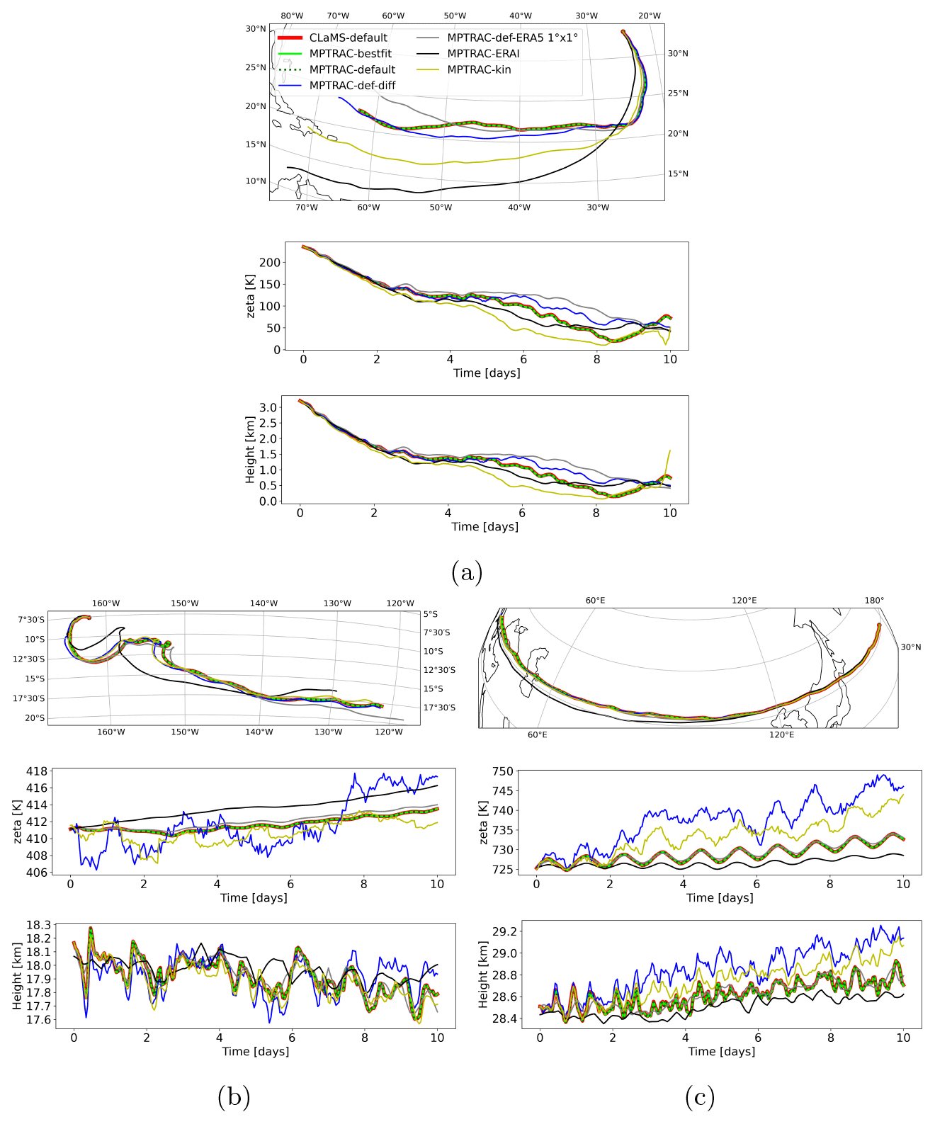
Figure 4 Examples of trajectories calculated 10 d forward from 1 July 2016. Different scenarios in three layers are shown: The (a) troposphere, (b) UTLS and (c) the lower stratosphere. For each trajectory the horizontal transport is shown in the upper panel. The vertical transport in the zeta coordinates and in log-pressure height is depicted below.

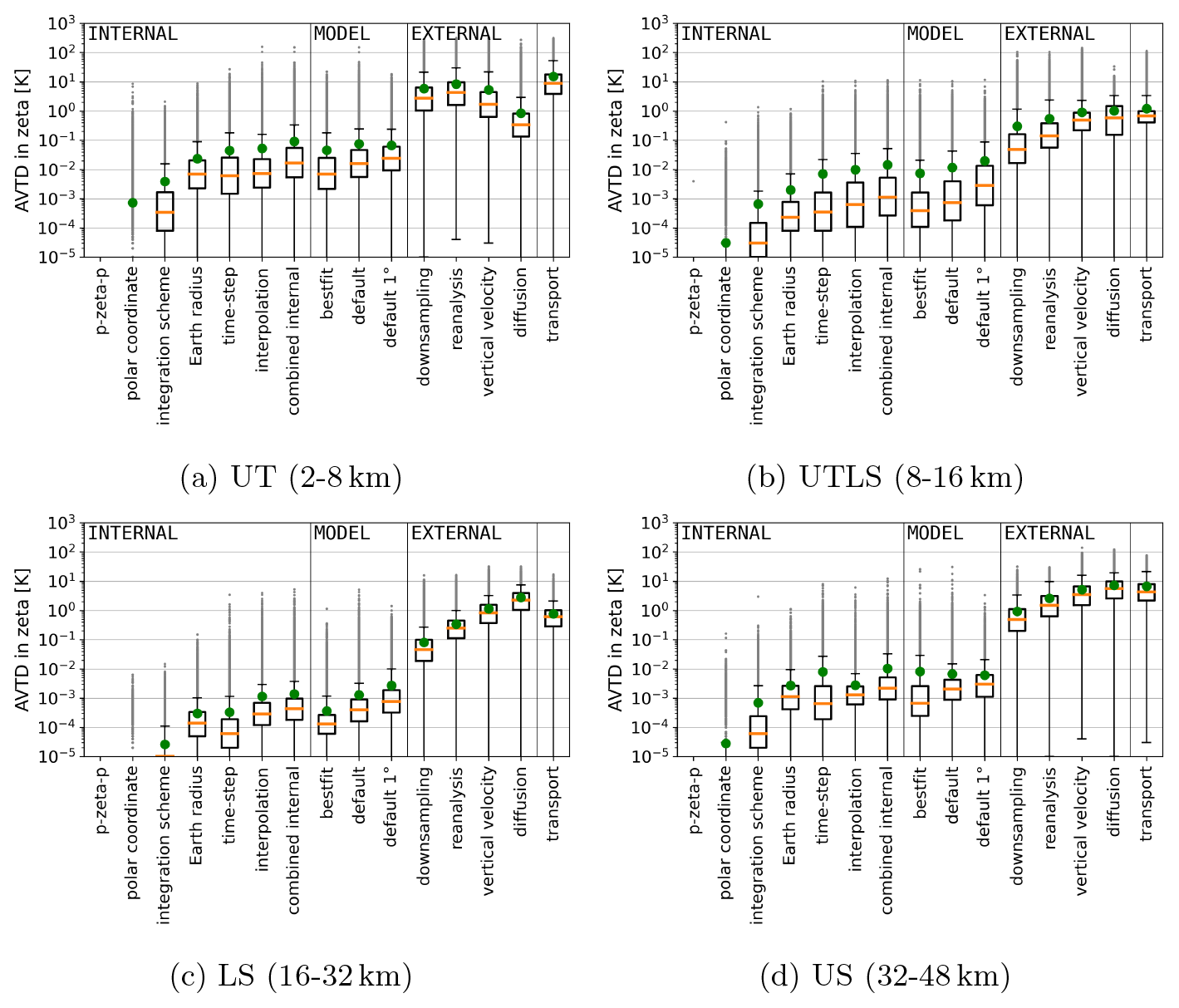
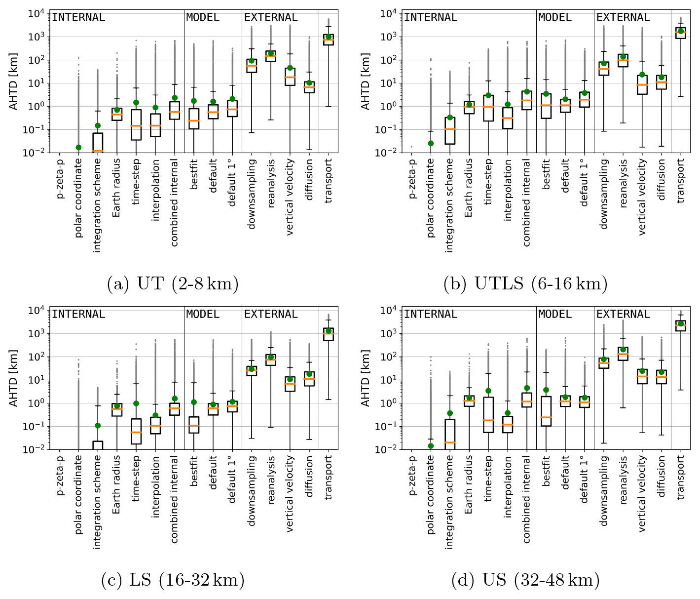
Figure 5 Different AVTDs in zeta coordinates after 1 d forward calculations for the entire ensemble of air parcels split into four height layers. The different uncertainty sources are defined in Table 2. The box plots show the median, quartiles (25 % and 75 %), the minimum and the 95 % quantile. Grey dots indicate deviations above the 95 % quantile. Green dots indicate the mean AVTDs. Deviations for the p-zeta-p transformation are lower than 10⁻⁵ K and do not show up here. The distinction between internal, model and external uncertainty sources is indicated by vertical lines.

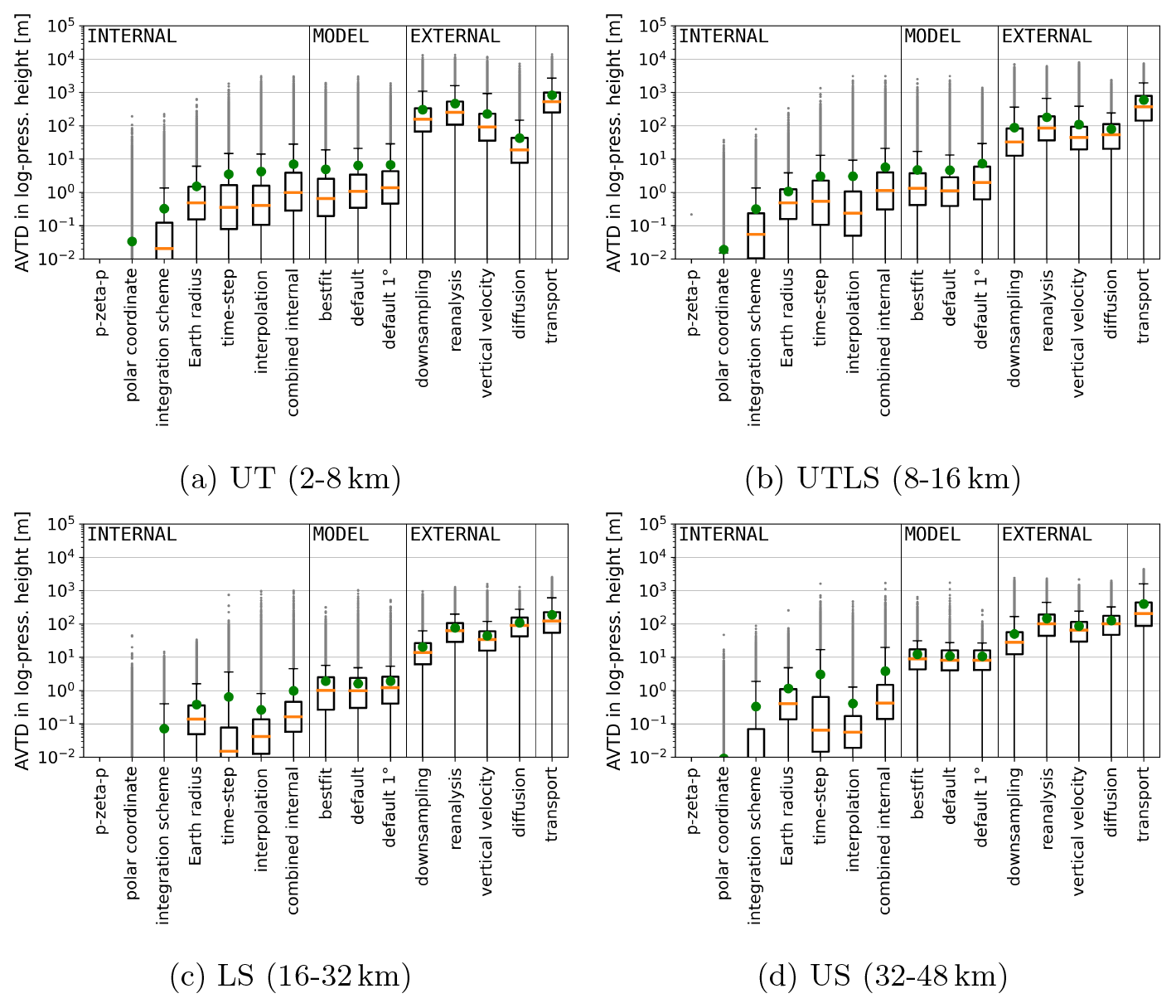
Figure 6 AVTDs in log-pressure heights after 1 d forward calculations for the entire ensemble of air parcels split in four height layers. The boxplots indicate quantiles as defined in Fig. 5.

Figure 7 Horizontal deviations quantified with the AHTDs after 1 d forward calculation for the entire ensemble of air parcels split in four height layers. The boxplots indicate quantiles as defined in Fig. 5.

3.2 Transport uncertainties over 1 d

Figure 5 shows statistics for vertical transport deviations after 1 d of calculations in hybrid zeta coordinates. Different height ranges are shown depending on the initial position of the air parcels. The height ranges are 2–8 km for the troposphere, 8–16 km for the UTLS, 16–32 km for the LS, and 32–48 km for the US. Throughout the troposphere and stratosphere, the model deviations measured by the median AVTD in the zeta coordinate are on the order of magnitude of the known combined internal uncertainties within MPTRAC (10⁻⁴ to 10⁻² K). This is true for the full ERA5 and ERA5 1° × 1° scenarios, although the uncertainties increase in the latter scenario (see Fig. 5: the labels “default” and “default 1°”).

Separately assessed, the variation of the Earth radius, the time step variation from 180 to 1800 s in the Runge–Kutta method, and the interpolation variation of MPTRAC are estimated to cause median AVTD lower than 10⁻² or 10⁻³ K, depending on the level (see Fig. 5: the labels “Earth radius”, “time step”, and “interpolation”). Since the change in the time step between 1800 and 180 s is only related to small deviations, time steps of 1800 s are still adequate (see Fig. 6: the label “time step”).

Only limited to trajectories in proximity to the poles, uncertainties due to the coordinate singularity must be considered. However, the transformation from spherical coordinates to the stereographic projection at high latitudes causes vertical deviations similar to deviations related to the selection of the integration method. If only air parcels that start at latitudes larger than 72° north or south are considered statistically, the median AVTD in zeta coordinates is on the order of 10⁻⁵ K for both the variation of the integration scheme and the horizontal coordinate. These larger deviations that are restricted to the pole also increase the mean AVTD in Fig. 5 over 10⁻⁵ K (see label “polar coordinate”). However, the horizontal median AHTD is still 1 order of magnitude larger for the variation of the integration scheme than for the horizontal coordinate in the polar region. The p-zeta-p transformation within MPTRAC, which combines pressure-based modules with zeta-based advection, causes transport deviations that are orders of magnitude smaller than the other uncertainty sources (below 10⁻⁵ K). Hence, the vertical coordinate transformation is the internal uncertainty of the least importance.

The CLaMS and MPTRAC models can also be configured to operate more similarly (i.e. using the same Earth radius and integration method and a similar interpolation method) so that the model uncertainty is substantially reduced (see Fig. 5: label “best fit”). Some minor differences in the interpolation scheme likely contribute to the remaining uncertainties.

Already, with the default configuration, there are model deviations for CLaMS and MPTRAC that are 1 to 3 orders of magnitude smaller than deviations resulting from external factors (see Fig. 5). For those large external uncertainties, the median AVTD values have orders of magnitudes of 10⁻² to 1 K. The importance of different external factors is different for the troposphere (i.e. below 8 km) and the stratosphere. In the stratosphere, diffusion from parameterized sub-grid-scale winds and turbulence leads to median AVTDs up to about 7 K after 24 h, exceeding the overall transport median AVTDs above 16 km (median AVTD between the initial positions and the end points, also labelled transport). The diffusion is accordingly the largest uncertainty at all layers, except between 2–8 km, where the reanalysis uncertainty is larger, followed by the uncertainty from downsampling and the vertical velocity. Between 2–8 km, the diffusion is also smaller because the parameterization of turbulent diffusion is restricted to horizontal directions. The second largest uncertainty above 8 km is given by the variation of the vertical velocity. For the vertical velocity variation, the median AVTD is on the order of 10⁻¹–1 K. Above 8 km, reanalysis variations, such as between ERA-Interim and ERA5, exhibit median AVTDs that are on the same order of magnitude as uncertainties from the vertical velocities but are smaller by a factor between 3 to 5 depending on height. Moreover, ERA5 1° × 1° shows a deviation compared to the full-resolution ERA5 that is 1 order of magnitude smaller than that from the variation of the reanalysis or the vertical velocity. In summary, the largest deviations in the zeta coordinate above 8 km are found from diffusion, followed by the vertical velocity, the reanalysis, and finally the downsampling of data. Hence, the implementation of diabatic transport has a significant impact on the calculations.

Figure 6 shows the same statistics as Fig. 5 but for log-pressure coordinates. For the height range between 2 and 32 km, the median AVTD in log-pressure coordinates between the two models in the default setup is ∼1 m. At higher levels (32–48 km), the median AVTD is 10 m. While the median AVTD between the models is around the same order of magnitude as the combined internal uncertainty between 2 and 16 km again (e.g. Fig. 6b), in log-pressure coordinates, the deviations are up to 2 orders of magnitude larger than the combined internal uncertainty for the levels above 16 km (e.g. Fig. 6d). This is a consequence of the transition from linear to logarithmic interpolation for pressure in CLaMS at isentropes higher than 500 K (around 20 km), which is not performed in the MPTRAC model.

Moreover, in the stratosphere, the median AVTD in log-pressure coordinates between the initial and final positions after 1 d (see label “transport”) is larger than the deviation from vertical diffusion in the pressure coordinate, which is in contrast to the median AVTD in zeta coordinates, because the transport in the UTLS is mostly isentropic and hence might cross multiple isobars but fewer isentropes (see Figs. 5 and 6: the labels “diffusion” and “transport” for the layers of the troposphere and lower stratosphere).

When the AHTDs are considered, qualitatively similar results to the vertical transport deviations are obtained. The horizontal model differences and combined internal uncertainties are of the order of 0.1 to 1 km after 1 d of calculations, while external uncertainties lead to absolute horizontal deviations of the order of 1 to 100 km (see Fig. 7). The difference between the initial and final positions is around 1000 km. For the internal horizontal deviations, the selection of the Earth radius becomes one of the largest internal uncertainties because it is used during the transformation from Cartesian to spherical coordinates. For the horizontal deviation, variations in the reanalysis and the downsampling become more important than uncertainty sources such as the vertical velocity because the latter do not alter horizontal velocities directly.

From an overall statistical perspective, as depicted by the Figs. 5 to 7, different layers show different uncertainties. To emphasize the vertical and hemispheric (i.e. seasonal) dependencies of transport uncertainties, Fig. 8a shows the hemisphere-wise vertical mean profiles for a selection of uncertainty sources. First, it is evident, again, that all uncertainties from external sources are orders of magnitude larger than uncertainties from internal sources and deviations between the models. Second, all uncertainties, except those due to parameterized diffusion, exhibit the largest absolute mean deviations in the troposphere (below 360 K). The smallest mean AVTDs in the zeta coordinate can be found between around 500 and 750 K, while the deviations above 600 K increase again with height. In comparison to absolute deviations, relative deviations (see Fig. 8b) show less dependency on height (the relative deviations are normalized to the sum of all incremental 1 h transport steps calculated with the default setup of CLaMS within each layer). While the troposphere has the highest relative uncertainties, the stratosphere shows lower relative uncertainties, which are also mostly independent of height. This indicates that the increase in the mean AVTD in the stratosphere is given because air parcels cross more levels at those heights during the transport process.

The profiles of the transport uncertainties are similar in the two hemispheres. However, if hemispheres are compared in more detail, the strongest relative internal uncertainties are found in the winter hemisphere, i.e. the Southern Hemisphere (see Fig. 8b). Absolute and relative uncertainties in the Southern Hemisphere, specifically in winter, are most likely to be much larger in the stratosphere due to the influence of the polar vortex and increased wave activity in winter. This seasonality was found by Hoffmann et al. (2019) with kinematic transport calculations as well. In particular, the integration time step becomes the dominant internal uncertainty source in the region of the polar vortex because high zonal velocities require shorter time steps for integration, which is not always fulfilled with 1800 s time steps for the ERA5 reanalysis. Larger deviations in horizontal directions lead to larger vertical deviations as well. The large hemispheric differences in the uncertainty explain the increased difference between the median and the mean deviations for the internal uncertainties and, in particular, the variation of the integration time step, seen in Figs. 5 to 7, in the stratosphere.

Moreover, the vertical profiles in Fig. 8 reveal that, throughout the stratosphere, the deviation from the variation of the vertical velocity is larger than the deviation from the variation of the reanalysis, which in turn is larger than the change from ERA5 to ERA5 1° × 1°. In particular, uncertainties from diffusion are lowest in the troposphere but increase sharply up to around the tropopause, where the diffusion becomes the largest normalized and absolute source of uncertainties. At higher levels, the normalized uncertainty from diffusion decreases slowly again back to normalized uncertainty ranges comparable to the normalized uncertainty from the variation of the vertical velocity. The normalized deviations given by the variation of the vertical velocity are reduced in the troposphere because the zeta coordinates are approximately equal to the sigma coordinates at lower levels. Overall, the results show that the implementation of diabatic vertical transport in MPTRAC has a significant impact, comparable to other external uncertainties.

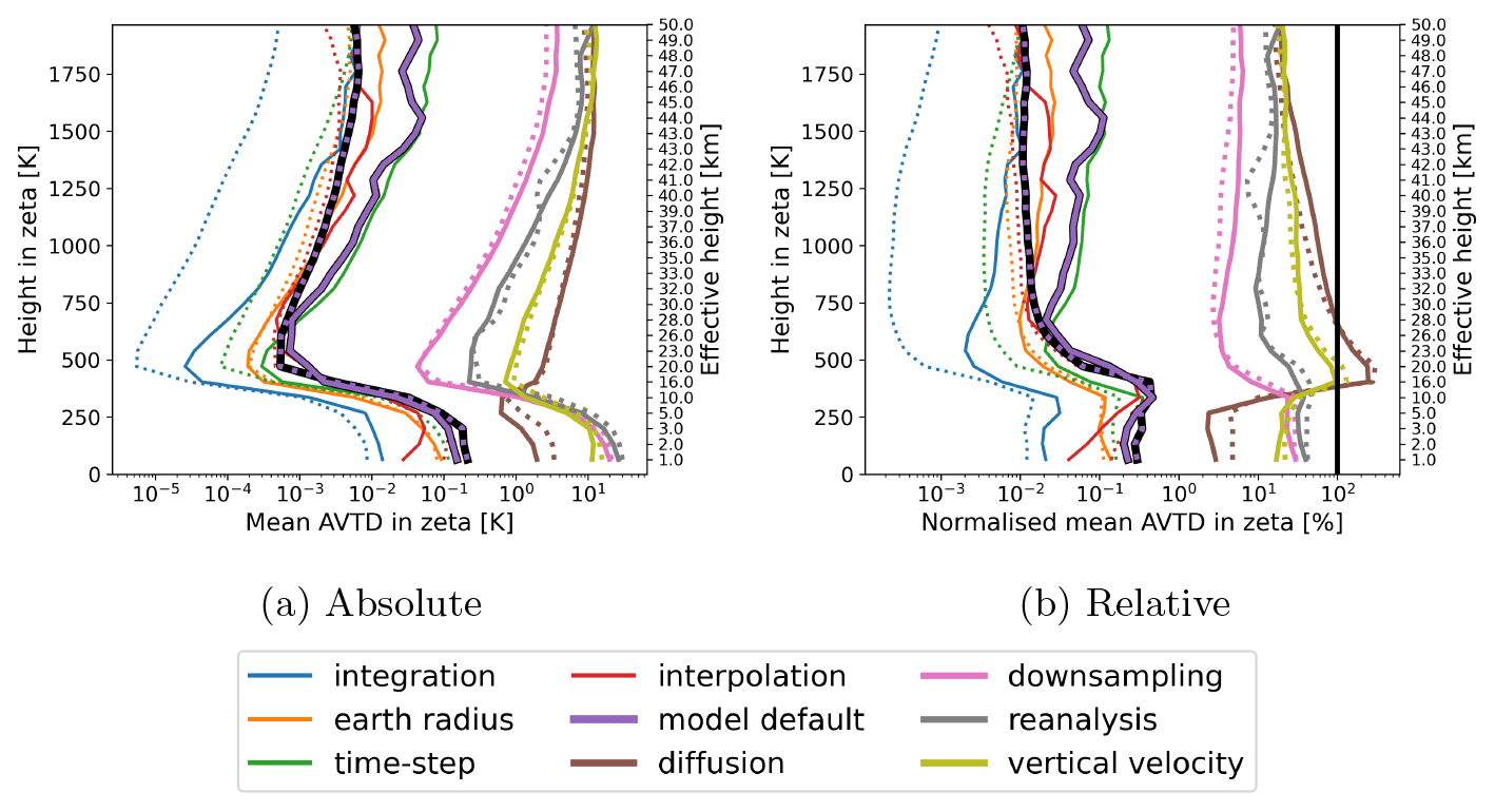
Figure 8 Smoothed vertical profiles of hemispheric average AVTD in zeta coordinates for different uncertainty sources (see Table 2 for the definitions). (a) Absolute values and (b) relative values, where the deviations are normalized for each level to the mean vertical path length calculated with the default setup of CLaMS (see “CLaMS-default” in Table 1). The black profile emphasizes the model difference for the models with default configuration in the summer hemisphere. The dotted lines indicate uncertainties in the Northern Hemisphere (boreal summer), and solid lines indicate uncertainties in the Southern Hemisphere (austral winter). The effective height is the average log-pressure height at a zeta level at the beginning of the calculations. The vertical black line in panel (b) marks 100 %.

3.3 Uncertainty growth during 90 d forward calculations

To investigate the uncertainty growth between the CLaMS and MPTRAC models and to better understand the model differences in the context of other uncertainties, trajectory calculations were performed for 90 d starting from 1 June 2016. Figure 9 displays the temporal evolution of the median AVTD between the two models, along with the downsampling, vertical velocity, reanalysis, and diffusion transport deviations. For the intercomparison of the two models, the default configurations of the models (see “model default” in Table 2) are used as they represent the usual uncertainty that has to be expected.

The model deviations and other transport uncertainties vary with height. In the troposphere, the median AVTD of the external uncertainties remains below 1 K only for a short period (a few hours to days) due to the strong mixing and convection. Subsequently, external uncertainties in this region grow rapidly by up to 4.3 K per day. In particular, the selections of the reanalysis, the vertical velocity, and downsampling cause fast divergence in the troposphere. The median model AVTD is smaller than uncertainties related to changes in reanalysis data, downsampling of the data, or parameterized sub-grid-scale winds and diffusion. The median AVTD between the two models remains below approximately 1 K for the first week. Subsequently, there is also a sharp increase (up to 2.2 K per day), reaching a median AVTD of about 55 K at 40 d of simulation time, where the different uncertainties reach a similar magnitude.

In the lower and upper stratosphere, the AVTD remains smaller because air parcels mainly move isentropically. Additionally, horizontal mixing is much less in most regions of the lower and upper stratosphere in contrast to the troposphere. The median model AVTD is, again, much smaller than all other uncertainty sources but now for the entire 90 d integration period. In the lower stratosphere, 50 % of the air parcels have a model AVTD lower than 1 K for approximately 2 months, and, afterwards, the deviation still increases slowly (not more than 0.16 K per day). In the upper stratosphere, the same criterion is met after around 34 d, also with a slow to moderate increase afterwards (not more than 1.2 K per day).

Uncertainties from the selection of the vertical velocity and the reanalysis are of similar importance. In the UTLS and at higher altitudes, the variation of the vertical velocity first shows slightly larger median AVTD than the variation of the reanalysis. However, after a couple of weeks, the median AVTD from the reanalysis selection is higher because the choice of the vertical velocity does not affect the horizontal wind speeds, as is the case for the choice of the reanalysis. The smallest transport uncertainty from external sources throughout the atmosphere is given by the ERA5 1° × 1° data because ERA5 1° × 1° has the same vertical resolution and similar horizontal velocities as the ERA5 reanalysis. Finally, in the UTLS, results lie in between the pure stratosphere and the troposphere, influenced by the transport of air parcels between the stratosphere and troposphere.

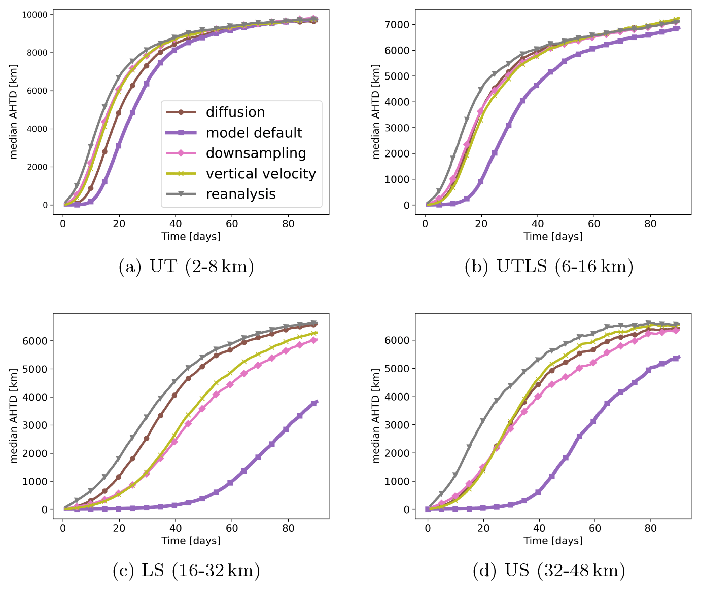
The differences between the two models have an impact on the horizontal distribution of the air parcels as well (Fig. 10). While the model median AHTD is less than 1000 km for 45 to 60 d in the stratosphere, it is less than 1000 km only for 15 to 20 d in the troposphere and UTLS. In the UTLS and troposphere, air parcel deviations reach an upper boundary, where further uncertainty growth stagnates for all scenarios, after around 40 d. In the stratosphere, this boundary is approached after 60 to 90 d for external uncertainty sources, while it is not completely approached by the model difference in this time period. Even the horizontal deviations for the scenario with ERA5 1° × 1° grow to be considerable throughout the atmosphere, indicating that air parcels are often not in good agreement with the ERA5 reanalysis.

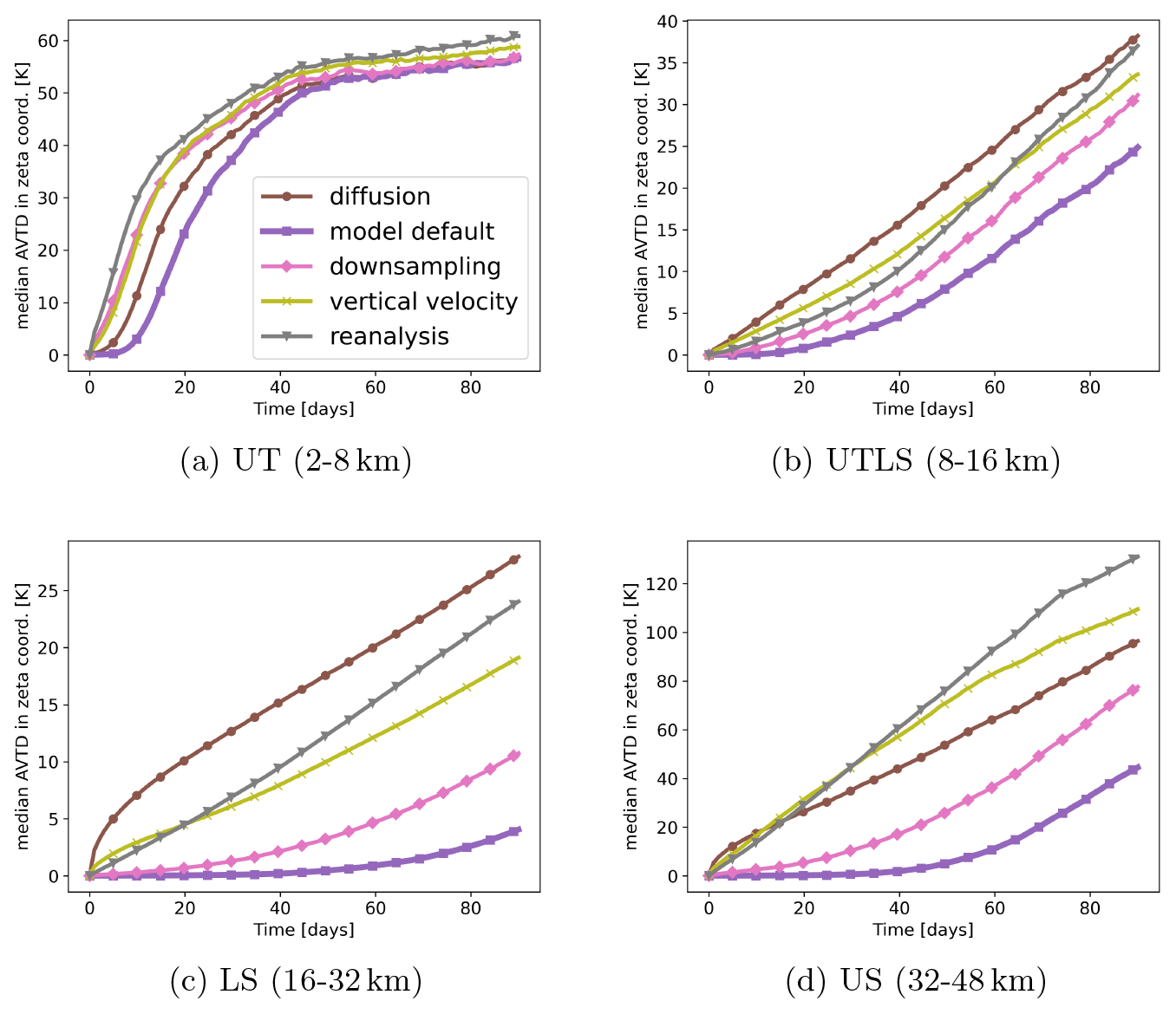
Figure 9 Evolution of the median AVTD in the zeta coordinate for different uncertainty sources for 90 d. The median AVTD between the two models is labelled “default”, as defined in Table 1. The starting date is 1 June 2016. The classification into the layers is done with the initial heights of the air parcels.

Figure 10 Evolution of the median AHTD of different uncertainty sources for 90 d. The median AHTD between the two models is labelled “default”, as defined in Table 1. The starting date is 1 June 2016. The classification into the layers is done with the initial heights of the air parcels.

3.4 Air parcel distribution on seasonal timescales

Since individual trajectories are not expected to agree over time periods of several months, the statistical distribution of air parcels after a 90 d integration period is used to quantify the differences between the models and the uncertainty related to external sources. The air parcels were initialized on 1 June 2016. For reference, the initial density of the air parcels is shown in Fig. 11a. Figure 11b shows the zonal mean distribution of air parcels after 90 d of forward calculations for the CLaMS model with its default configuration. After 90 d, the density is highest around the vertical level of 450 K, where most of the air parcels have been transported to within the shallow and deep branches of the Brewer–Dobson circulation (BDC). Air parcels also accumulate below the tropopause and near the surface below 2 km (where the models are configured to terminate the air parcel trajectories). Sub-grid-scale process, such as convection, that would be required to reach a well-mixed troposphere are not parameterized in the calculations. Therefore, the accumulation of air parcels is a consequence of up- and downward transport limited to the resolved mean flow of the troposphere, combined with the tropopause as an upper transport barrier and the ground as the lower transport barrier.

Furthermore, more air parcels are leaving the Northern Hemisphere than entering it in the calculations, i.e. the cross-equatorial flow in the UTLS increases the air parcel density in the Southern Hemisphere in relation to the Northern Hemisphere. Since the air parcels were initialized on 01 June 2016, the simulation describes the boreal summer conditions. As indicated by averaged trajectories in Fig. 11b, the hemispheric asymmetric distribution of air parcels is mostly related to the strength of the southern hemispheric, shallow branch of the BDC that is located between 40° S and 5° N in latitude and crosses the Equator (see Appendix A for details about the average trajectories).

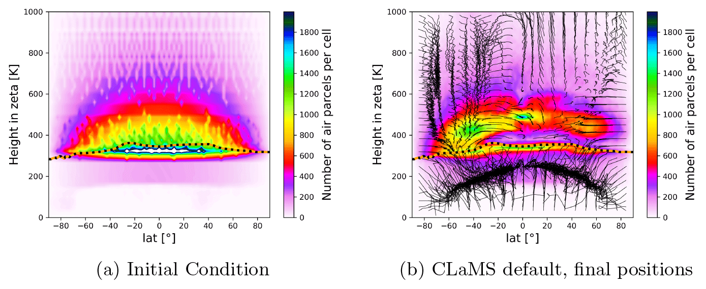
Figure 11 Initial and final air parcel distribution after 90 d when calculated with the CLaMS default setup. Black lines show box-wise averaged trajectories to indicate the average circulation of the trajectories. The dotted orange line indicates the 90 d average tropopause.

The global distribution of air parcels as simulated with MPTRAC is almost identical to the distribution as simulated with CLaMS, as can be seen in Fig. 12a, where the bias between the air parcel distributions of both models is shown, along with contour lines of air parcel frequencies after 90 d forward calculations. The contour lines of the air parcel frequencies align very well around the tropopause and at higher levels around 500 K. Overall, there is no significant bias between the air parcel distribution of the two models. Except for statistical noise, the simulation results of CLaMS and MPTRAC are in excellent agreement. This is in distinct contrast to biases found for other known uncertainties (e.g. from reanalysis, vertical velocity, and downsampling), as will be discussed below.

When the diffusion module (see Fig. 12b) is switched on in MPTRAC, the air parcel distribution as found without diffusion is mostly reproduced. However, the air parcel distribution shows “smoothed peaks” between 400 and 600 K; i.e. air parcels are more strongly scattered around the peaks. For example, in Fig. 12b, the circumferences of the green contours shrink in comparison to those of the black contours. Moreover, fewer air parcels are found in the height region where the frequency of air parcels peaks for the default scenarios of MPTRAC and CLaMS (around 450 K), whereas the frequencies are increased at the neighbouring levels. The result indicates that the mean distribution is not affected by the sub-grid-scale diffusion, except for a smoothing effect. It is also shown in the Appendix that the diffusion causes large cross-isentropic dispersion (see Fig. B2 in the Appendix).

The downsampling of the ERA5 data (see Fig. 12c) has only a minor impact on the distribution of air parcels above the tropopause. The largest differences can be found at the tropical tropopause and in the troposphere. With ERA5 1° × 1°, more air parcels remain located within the troposphere after 90 d. This is presumably a consequence of reduced vertical transport in convective events in the ERA5 1° × 1° in comparison to the full-resolution data, which would be in agreement with other studies (e.g. Hoffmann et al., 2023b). With weaker vertical transport, more air parcels remain in the troposphere, and fewer air parcels are transported downward into the model boundary layer, where they are terminated.

With ERA-Interim, qualitatively very different results are found (see Fig. 12d). The BDC transport is faster with ERA-Interim than with ERA5 between levels around 400 to 600 K. Hence, more air parcels are transported from around 400 K to around 600 K in ERA-Interim. At the same time, transport at higher levels than 600 K is slower with ERA-Interim than with ERA5, which decreases the air parcel number relative to ERA5 above 700 K. The upward transport in the upper part of the shallow branch is faster in ERA-Interim than in ERA5 as well (see also Appendix A1d). Hence, more air parcels are found at higher altitudes around latitudes of 45° S with ERA-Interim. These results are in agreement with the findings of Ploeger et al. (2021), who studied the climatological zonal structure of diabatic velocities in ERA5 and ERA-Interim. Additionally, more air parcels are found between the 400 K level and the tropopause with ERA-Interim than with ERA5. The combination of uncertainties between the two reanalyses complicates their intercomparison in the UTLS.

The biases between simulations with diabatic and kinematic vertical velocities in ERA5 are of similar size compared to the biases between simulations with ERA-Interim and ERA5 (see Fig. 12e). With kinematic vertical velocities, the upward transport in the BDC is as fast as with the diabatic transport scheme or even faster for levels between 400 and 900 K (see also Fig. A1e). Therefore, fewer air parcels can be found between 400 and 500 K compared to the diabatic vertical velocities. Additionally, the bias roughly resembles the bias found for the scenario with parameterized diffusion and hence indicates an increased dispersion of the air parcels. Indeed, diagnosed cross-isentropic dispersion is increased with kinematic calculations. However, the differences between diabatic and kinematic trajectories, in terms of vertical transport and dispersion, are significantly reduced in ERA5 in comparison to ERA-Interim (see Appendix B).

With kinematic velocities, increased air parcel numbers can be found closely above the tropopause as well in comparison to the diabatic calculations. This possibly indicates increased transport across the tropopause from below. However, for the kinematic velocities, higher numbers of air parcels are found in the troposphere because the applied criteria for excluding air parcels from further transport (reaching the level where the zeta coordinate is zero) are not fulfilled. Therefore, the increase in air parcels closely above the tropopause could be a consequence of higher air parcel numbers remaining in the troposphere as well.

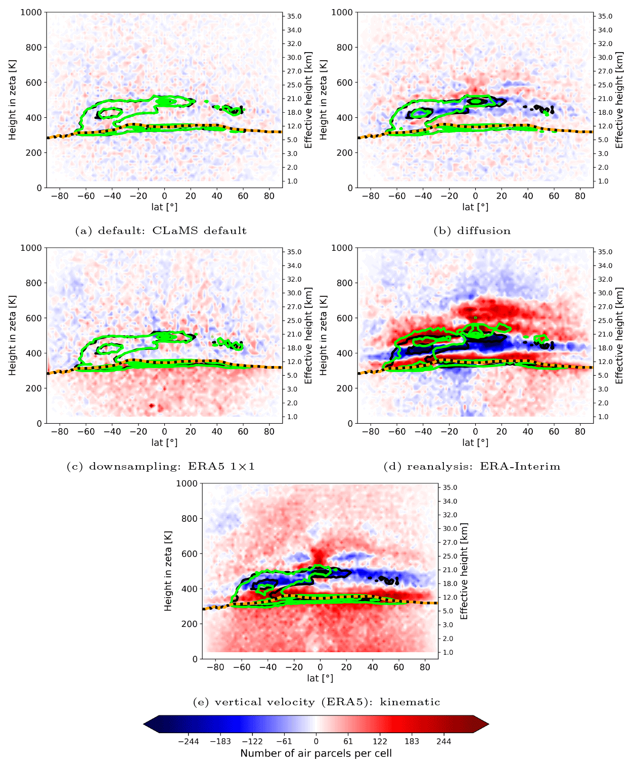
Figure 12 Zonal mean bias of the air parcel distributions after 90 d between the default MPTRAC scenario and a selected scenario. Positive bias indicates lower frequency with the default MPTRAC scenario and higher frequency with the respective scenario. The dotted orange line is the 90 d average tropopause. The green contours show the 600, 1000, and 1400 air parcel numbers per cell contour of the air parcel distributions for intercomparison with the scenarios of (a) CLaMS default, (b) diffusion, (c) downsampling (ERA5 1° × 1°), (d) reanalysis (ERA-Interim), and (e) vertical velocities (kinematic calculations). The black contours indicate the same contour lines but for the MPTRAC default scenario.

3.5 Conservation of dynamical tracers in the stratosphere

In the stratosphere, the potential temperature (θ) and the potential vorticity (PV) are approximately conserved. To assess the conservation of dynamical tracers in different scenarios with the newly implemented diabatic transport scheme in MPTRAC, Fig. 13a shows the 10 d evolution of the mean RTCE of the PV in the stratosphere, starting from 1 June 2016. Only air parcels with an initial height above 360 K, the approximated level of maximum convective outflow, are analysed. The potential temperature and PV are calculated with the modules of the MPTRAC model along the trajectories. The mean conservation error after 1 d varies between 10 % and 13 %, depending on the scenario. After 10 d, the mean RTCE increases to values between 25 % and 28 %. The differences between the different scenarios remain moderate, with slightly lower PV conservation errors with the ERA5 reanalysis and diabatic velocities as implemented in MPTRAC. To show the significance of the increase, it has been compared with the unresolved parameterized sub-grid-scale diffusion: the difference between the diabatic calculations with ERA5 and the kinematic velocity scheme is almost as large as the difference between the kinematic scenario and the scenario with parameterized sub-grid-scale winds and diffusion. Figure 13b shows the evolution of the conservation error of the potential temperature. The mean RTCE is very similar (±0.1 %) for all scenarios, except for the scenario with parameterized diffusion and sub-grid-scale wind fluctuations.

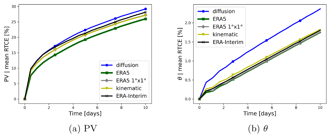
Figure 13 Evolution of the mean RTCE of (a) PV and (b) θ for different scenarios within a 10 d period. All scenarios are driven with MPTRAC. See the scenarios in Table 1 between MPTRAC-default and MPTRAC-def-erai for further details. The starting date is 1 June 2016. Only air parcels with an initial altitude above 360 K are considered.

4 Conclusions

In this study, a diabatic transport scheme based on hybrid zeta coordinates was implemented in the MPTRAC Lagrangian transport model. This work's intention is to enable a transition from the CLaMS Lagrangian transport framework towards a code which enables shared-memory multiprocessing with CPUs or offloading to GPUs and which is, hence, more suitable for recent and upcoming HPC architectures. To evaluate the implemented scheme in MPTRAC, we conducted simulations using approximately 1.4 million globally distributed air parcels in the troposphere and stratosphere, following an initialization method commonly employed with CLaMS. Trajectory forward calculations were performed for the boreal summer of 2016. In the evaluation, the model differences were put in the context of various other uncertainty sources in Lagrangian transport calculations. Consequently, the model differences between CLaMS and MPTRAC were presented within a hierarchy of uncertainties associated with Lagrangian transport models.

The key differences between the two Lagrangian models relate to their approach for the interpolation of the driving meteorological data and the numerical integration scheme. Although both models apply four-dimensional linear interpolations, CLaMS performs them directly in spherical coordinates, while MPTRAC performs them in Cartesian coordinates. As a default, CLaMS uses the classical fourth-order Runge–Kutta scheme with 1800 s integration steps for numerical integration in order to run with feasible computational costs. MPTRAC employs the mid-point scheme with 180 s integration time steps. At a time step of 180 s, both integration schemes deliver very similar results. The residual differences between the models are likely caused by remaining differences in the interpolation. For improved agreement, CLaMS and MPTRAC should use the identical Earth radius. Further alignment of the interpolations could achieve even better agreement.

Despite the conceptual model differences, it was demonstrated that, for a period of 1 d, the discrepancy between CLaMS and MPTRAC air parcel vertical positions is comparable to the combined internal uncertainties associated with different Earth radii, interpolation methods, numerical integration schemes, and selected integration time steps. These deviations are, at a minimum, around 1 order of magnitude smaller than the uncertainties arising from external sources, such as differences between reanalysis data sets, downsampling of the ERA5 reanalysis data, and unresolved fluctuations of the wind fields. Thus, the analysis of the model differences indicates an excellent agreement of CLaMS and MPTRAC within the boundaries of known internal and external uncertainties. This also holds in the regions of the most notable differences, including the troposphere and the winter stratosphere with the polar vortex.

The uncertainty growth between the models and from external sources for 90 d was also estimated. The vertical transport uncertainty remains less than around 1 K for several weeks, in particular in the stratosphere. The transport deviation between the models is significantly smaller than the deviation caused by external sources of uncertainty for the entire 90 d time period. In particular, large uncertainty growth from variations of the vertical velocity (diabatic to kinematic) shows that the implementation of the diabatic transport scheme in MPTRAC has a significant impact on the transport of air parcels.

For a global, long-term study of trace gases, the statistical distribution of air parcels in the UTLS, as opposed to individual trajectory errors, becomes more important. In their present configurations, both models distribute air parcels very similarly even after 90 d, supporting the hypothesis that the models provide similar long-term tracer fields. Accordingly, no biases in the air parcel distributions were found between the two models. In contrast, known external uncertainties caused significant biases in the trajectory calculations over the 90 d integration period.

The diabatic transport calculations show that transport within the BDC is faster with ERA-Interim than with ERA5 between 400 and 600 K but slower for higher levels. This is in agreement with recent climatological and regional studies of vertical velocities and transport in the upper troposphere and stratosphere (Ploeger et al., 2021; Vogel et al., 2024).

Differences between calculations with diabatic and kinematic vertical velocities, even with ERA5, are still on the order of reanalysis differences, further corroborating the implementation of the diabatic scheme in MPTRAC. However, the difference between diabatic and kinematic calculations is significantly reduced with ERA5 in comparison to ERA-Interim with regard to the vertical transport in the circulation of the lower stratosphere but also concerning the cross-isentropic dispersion in the tropical lower stratosphere.

Furthermore, since model and internal uncertainties of the trajectory models are much smaller than uncertainties due to downsampling of ERA5 data, it can be concluded that using ERA5 1° × 1° for the sake of the acceleration of computations has considerable side-effects, in particular in the troposphere. This stresses the important role of the spatio-temporal resolution of the global reanalysis fields next to other improvements in the forecast models and data assimilation schemes used to produce the reanalyses. Making Lagrangian models ready for operation with higher-resolution meteorological data (as intended with MPTRAC) is fundamental to fully exploit the opportunities of next-generation reanalyses. Alternatively, applying better downsampling or data compression methods might be an option for future work.

In conclusion, this evaluation demonstrates that MPTRAC can replace CLaMS' trajectory module with the newly implemented hybrid zeta coordinates and diabatic transport scheme. The evaluation found no significant biases or deviations between the models but highlights the significance of using the high-resolution ERA5 reanalysis combined with diabatic transport. Furthermore, now that the implementation has been validated, additional performance analyses and optimizations can be carried out.

Appendix A: Circulation in the UTLS

To clarify the differences in the circulation patterns during the 90 d integration period, Fig. A1 shows the box-wise averaged trajectories. With a grid (around 8° × 32 K) using the initial positions, air parcels have been sorted into groups. Bins with less than 100 air parcels are excluded. The average position of this group of air parcels, following them in time, defines the box-wise averaged trajectory. Then, the vector that connects the end point of the MPTRAC default scenario with the end point of the compared scenario is calculated.

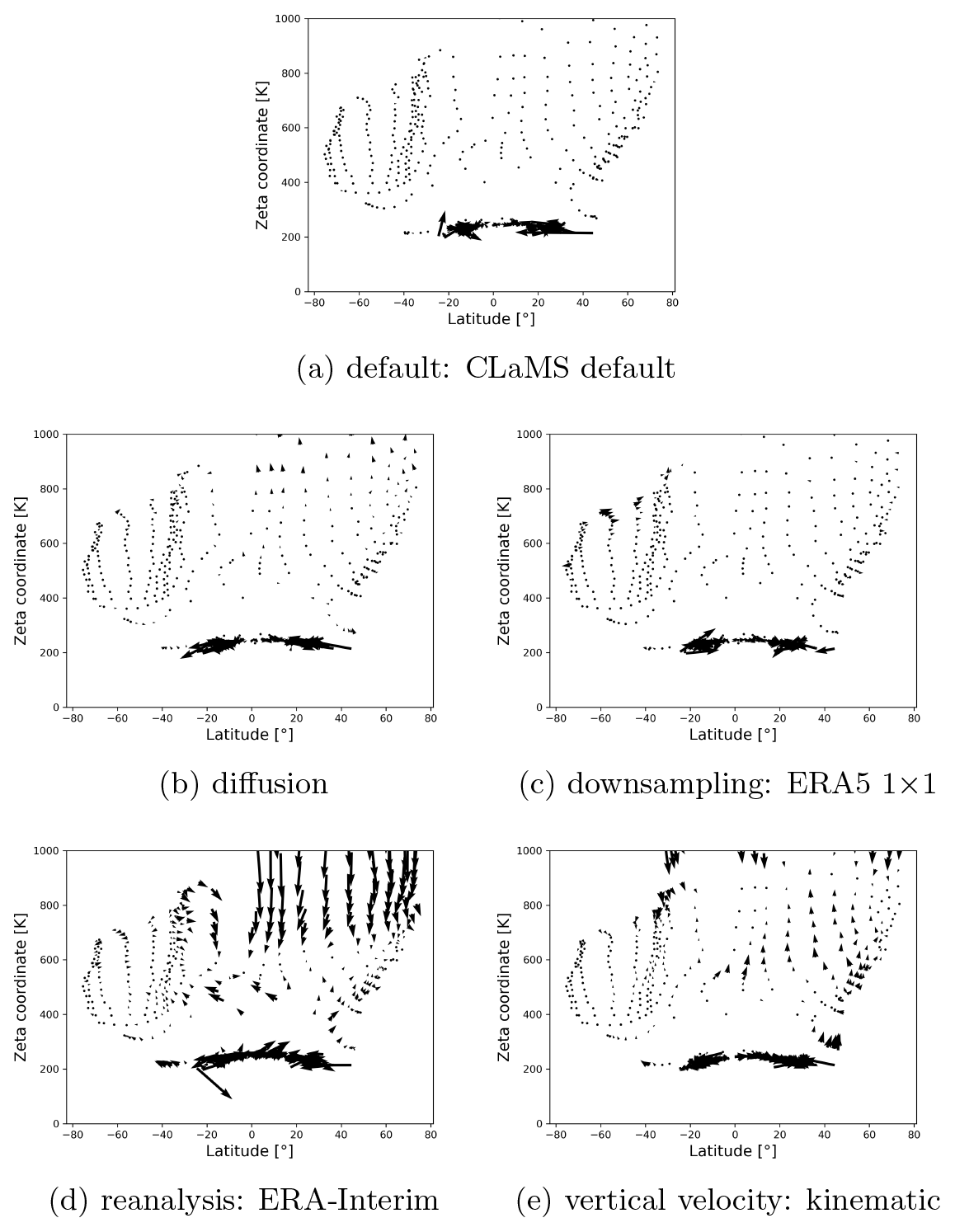
Figure A1 Vector differences of end points of box-wise averaged trajectories for the 90 d transport calculations in the UTLS and troposphere. The arrows indicate how the final MPTRAC-default positions have to be adjusted to agree with the respective scenario. Accordingly, they show the trajectory biases.

Appendix B: Cross-isentropic dispersion of air parcels

The agreement between kinematic and diabatic trajectories might differ from reanalysis to reanalysis in terms of the general circulation and cross-isentropic dispersion of air (Ploeger et al., 2011; Hoffmann et al., 2019; Legras and Bucci, 2020; Ploeger et al., 2021). Figure B1 shows biases after 90 d forward calculations between the kinematic and diabatic vertical velocity approach in ERA5 and ERA-Interim. The transport biases between kinematic and diabatic trajectories are significantly decreased with ERA5 in comparison to ERA-Interim between 300 and 600 K. The height of the air parcels varies substantially more with ERA-Interim than with ERA5 after 90 d of calculations (see black and green contours in Fig. B1).

The cross-isentropic dispersion of air parcels can be quantified with the variance of the potential temperature (Sparling et al., 1997; Ploeger et al., 2011) of an air parcel ensemble initialized at one isentropic level at a specific time: $\langle \mathit{\delta }{\mathit{\theta }}^{\mathrm{2}}\rangle =\langle {\left(\mathit{\theta }-\langle \mathit{\theta }\rangle \right)}^{\mathrm{2}}\rangle$. The brackets 〈 〉 symbolize the average over the air parcel ensemble. For levels higher than 360 K, the zeta coordinate approximates isentropic coordinates, i.e. potential temperatures, and hence can be used to estimate the dispersion as well. Since the initial position of the air parcels is given at zeta levels, each of these levels contains an ensemble of air parcels that can be used to calculate a separate variance. Similarly to Ploeger et al. (2011), only the air parcels that are initialized in the equatorial region are considered here (latitudes between ±30°) and remain in there. Figure B2 summarizes the variance calculated at different zeta levels in the range between 300 and 1000 K.

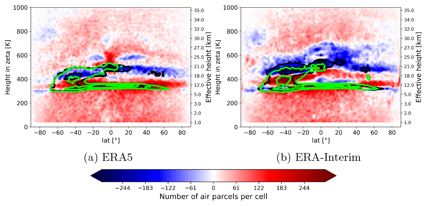
Figure B1 Intercomparison of air parcel distributions and biases inferred from diabatic (black contours) and kinematic (green contours) calculations for ERA5 (a) and ERA-Interim (b). The colour bar indicates the bias as used in Fig. 12. Here, positive bias indicates more air parcels with the kinematic scenario than with the diabatic scenario. All calculations are done with MPTRAC.

The kinematic calculations with ERA5 still have a higher dispersion in comparison to the diabatic calculations, which supports the implementation of the diabatic scheme in MPTRAC. The variance is around 3 times higher with the kinematic calculations between 400 and 550 K. However, the dispersion by parameterized turbulent diffusion and sub-grid-scale wind fluctuations is much higher (see Fig. B2). Finally, it can be noted here that the two models agree highly with regard to dispersion. The differences between calculations with ERA5 and the low-resolution ERA5 1° × 1° are small as well.

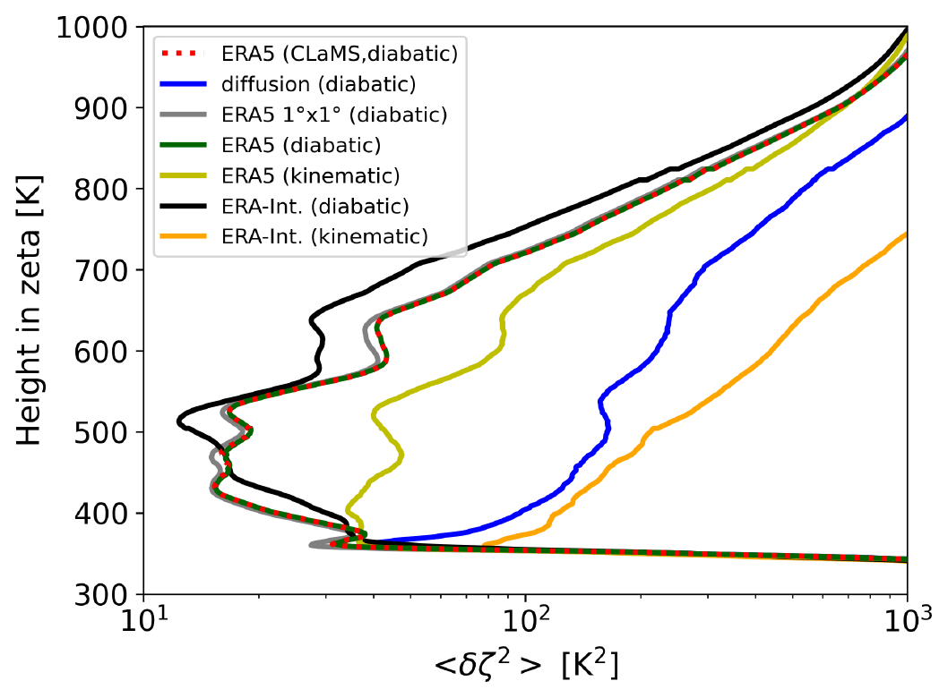
Figure B2 Profiles of the zeta variance 〈δζ²〉 after 10 d as a measure of the cross-isentropic dispersion. All scenarios are calculated with MPTRAC, except ERA5 (CLaMS, diabatic). The profiles for the scenarios ERA5 (diabatic) and ERA5 (CLaMS, diabatic) overlap with each other. For the definition of the MPTRAC scenarios, see also Table 1 from label “MPTRAC-default” to label “MPTRAC-def-erai-kin”.