Implementation of a Simple Actuator Disk for Large-Eddy Simulation in the Weather Research and Forecasting Model (WRF-SADLES v1.2) for wind turbine wake simulation

In this study, we present the development of a Simple Actuator Disk model for Large-Eddy Simulation (SADLES), implemented within the Weather Research and Forecasting (WRF) model, which is widely used in atmospheric research. The WRF-SADLES model supports both idealized studies and realistic applications through downscaling from realistic data, with a focus on resolutions of tens of meters. Through comparative analysis with the Parallelized Large-eddy Simulation Model (PALM) at resolutions of 10 and 30 m, we validate the effectiveness of WRF-SADLES in simulating the wake characteristics of a 5 MW wind turbine. Results indicate good agreement between WRF-SADLES at 30 m resolution and 10 m resolution and the PALM model. Additionally, we demonstrate a practical case study of WRF-SADLES by downscaling ERA5 reanalysis data using a nesting method to simulate turbine wakes at the Alpha Ventus wind farm in the south of the North Sea. The meso-to-micro downscaling simulation reveals that the wake effect simulated by WRF-SADLES at the FINO1 offshore meteorological mast station aligns well with the cup anemometer and lidar measurements. Furthermore, we investigate an event of farm-to-farm interaction, observing a 16 % reduction in ambient wind speed and a 38 % decrease in average turbine power at Alpha Ventus due to the presence of a wind farm to the southwest. WRF-SADLES offers a promising balance between computational efficiency and accuracy for wind turbine wake simulations, making it valuable for wind energy assessments and wind farm planning.

1 Introduction

Wind energy has become increasingly important due to the pressing need to address climate change and reduce our reliance on fossil fuels. It is crucial to have a deep understanding of the complex interaction between wind turbines and the atmospheric boundary layer (ABL) for effective wind energy assessment and wind farm construction planning. In particular, the wake created behind upstream turbines can have a significant impact on the performance of downstream turbines, resulting in reduced power production and increased turbulence (Porté-Agel et al., 2020; Bakhoday-Paskyabi et al., 2022a). Large-eddy simulation (LES) is a powerful tool that can simulate ABL turbulence with high spatial and temporal resolution, making it an invaluable resource for studying turbine wakes and their interaction with the ABL (Breton et al., 2017).

To model the turbine wakes, various methods exist with different levels of accuracy and computational cost. The most accurate but computationally expensive are the actuator surface (AS) and actuator line (AL) models. These models typically employ blade element (BE) theory (Burton et al., 2011) to calculate the thrust and torque on the turbine blades. A less computationally demanding approach is the actuator disk with rotation (AD+R) model. This model represents the turbine blades as a permeable disk extracting energy from the wind through axial and azimuthal forces. AD+R models often utilize BE theory or combine it with momentum theory (i.e., BEM theory; Göçmen et al., 2016; Ledoux et al., 2021). The simplest form is the actuator disk without rotation (AD), which only considers the axial force and typically uses momentum theory (Rankine, 1865). These turbine wake models have been implemented in various large-eddy simulation (LES) models, including EllipSys3D (AL) (Göçmen et al., 2016), MITRAS (AD+R) (Salim et al., 2018), the Simulator for Wind Farm Applications (SOWFA) (AL) (Fleming et al., 2014; Churchfield et al., 2016), and the Parallelized Large-eddy Simulation Model (PALM) (AL, AD, AD+R) (Witha et al., 2014; Maronga et al., 2015, 2020). For applications where detailed near-wake structures are not essential, AD+R and AD methods are preferred due to their lower computational cost, easier implementation, and sufficient accuracy for far-wake information (Breton et al., 2017).

Besides the accuracy of the turbine wake methods, a realistic ABL plays a crucial role in wake simulations. The processes that affect wind farms range from macro- and mesoscale weather phenomena down to the microscale of turbulence in the ABL (Porté-Agel et al., 2020). Given this multi-scale nature, a meso-to-micro numerical downscaling could be useful in simulating the ABL–turbine interaction realistically and understanding its underlying mechanisms (Muñoz-Esparza et al., 2014; Bakhoday-Paskyabi et al., 2022a). To incorporate realistic ABL conditions, one can use the meso–micro offline coupling approach; i.e., the output of a mesoscale model is used as the driven boundary condition for the dedicated LES models (e.g., Wang et al., 2020; Lin et al., 2021; Bakhoday-Paskyabi et al., 2022b; Onel and Tuncer, 2023). However, this approach depends on the frequency of the mesoscale model output, which is often not enough for short-timescale processes. The second approach, online coupling, uses a meso–micro coupled model system, where a mesoscale model and an LES model are coupled through a coupling interface. While the online coupling approach provides a seamless downscaling, it is more difficult to implement than the offline approach. The third approach, nested downscaling, involves a single model that can handle the downscaling naturally through a system of nested domains where the inner domains can be configured to run in LES mode. For example, the Consortium for Small-scale Modeling (COSMO) model (Baldauf et al., 2011) and the Weather Research and Forecasting (WRF) model (Skamarock et al., 2021) provide this capability.

The WRF model is open-source software that is highly popular in the atmospheric research community for studying a wide range of atmospheric processes, from idealized studies to real-world applications. It facilitates a meso-to-micro nested downscaling framework capable of simulating turbine wakes under realistic atmospheric boundary layer (ABL) conditions (Muñoz-Esparza et al., 2014; Bakhoday-Paskyabi et al., 2022a; Ning et al., 2023). Several WRF implementations include the effects of wind farms and wind turbines (e.g., Fitch et al., 2012; Volker et al., 2015; Mirocha et al., 2014; Kale et al., 2022), which can be grouped into wind farm parameterization (WFP) and wind turbine model (WTM).

The WFP approaches (Fitch et al., 2012; Volker et al., 2015) are commonly used to study the collective effects of wind turbine wakes on the ABL and the interactions between wind farms (e.g., Pryor et al., 2020; Fischereit et al., 2022). One advantage of these approaches is their low computational cost and ease of implementation. For example, the method used by Fitch et al. (2012) only requires the thrust and power curve data from turbine manufacturers. However, due to the limitation of the target horizontal resolutions, which must be at least 3 to 5 rotor diameters (Fischereit et al., 2022), the WFP cannot explicitly resolve individual turbine wakes or turbine-to-turbine interactions. This may result in inaccurate evaluations of wakes behind wind farms (Lee and Lundquist, 2017). On the other hand, the implemented general actuator disk (GAD) model in WRF (Mirocha et al., 2014; Kale et al., 2022) employs the AD+R method based on BEM theory. However, the GAD model requires more information about the turbine (such as blade profiles and aerodynamic characteristics), the generator speed, and blade pitch control, which may sometimes be confidential and not publicly available. Further, the WRF-GAD implementation's source code has not been released publicly, limiting its use for the scientific community, despite the WRF being open source.

To address these limitations, this study introduces a new wind turbine wake model named the Simple Actuator Disk for Large-Eddy Simulation (SADLES) within the WRF framework. Unlike WRF-GAD, WRF-SADLES utilizes traditional momentum theory that requires only basic information about the turbines, such as their thrust and power curves, similar to the WFP model by Fitch et al. (2012). However, in contrast to Fitch et al. (2012), WRF-SADLES is capable of explicitly resolving turbine wakes, similar to WRF-GAD. While many WRF-GAD applications typically employ fine resolutions of a few meters (e.g., Mirocha et al., 2014; Arthur et al., 2020; Kale et al., 2022), such high resolutions are computationally expensive for realistic downscaling problems involving large domains with multiple wind farms. Therefore, WRF-SADLES is also tested with coarser resolutions (specifically, 30 and 40 m) to achieve a more practical balance between computational cost and wake resolution. To facilitate its application within the meso-to-micro downscaling approach, we have also implemented the cell perturbation method (Muñoz-Esparza et al., 2014), which allows faster development of turbulence within nested domains. The WRF-SADLES code package is an open-source software suite encompassing both the SADLES module and the cell perturbation module. Its development aims to eventually be integrated into the official WRF repository, fostering further open research within the weather forecasting community.

To validate the WRF-SADLES model, firstly, an idealized case is used to compare the simulations of a 5 MW wind turbine from WRF-SADLES with the PALM model. The reason for selecting PALM was that it includes a wind turbine model that uses the AD+R method based on BE theory (Dörenkämper et al., 2015), which is comparable with the WRF-GAD model. Moreover, the PALM model has been shown to agree well with more sophisticated wake models and observations (Witha et al., 2014; Vollmer et al., 2015; Dörenkämper et al., 2015; Bakhoday-Paskyabi et al., 2022a, b). In addition, we demonstrated a more realistic application of WRF-SADLES by downscaling the ERA5 reanalysis data (Hersbach et al., 2020) to 40 m resolution around the Alpha Ventus wind parks, enabling us to investigate the effects of turbine-to-turbine and farm-to-farm interactions. The simulations are then compared with the observational data recorded at the FINO1 offshore meteorological mast station.

The rest of this paper is structured as follows. Section 2 details the WRF-SADLES method and implementation. Section 3 presents an idealized single-turbine simulation compared with the PALM model. Section 4 showcases a multi-scale downscaling application with multiple wind farm simulations. Section 5 concludes by summarizing the key findings and discussing the potential applications and limitations of the WRF-SADLES model.

2 Methods

2.1 The Simple Actuator Disk for Large-Eddy Simulation

The actuator disk (Anderson, 2020) is a hypothetical surface perpendicular to the wind flow that extracts energy continuously from the ambient wind through the work of the thrust force:

$$\begin{array}{}\text{(1)}& {\mathit{F}}_T=-{\displaystyle \frac{\mathrm{1}}{\mathrm{2}}}\mathit{\rho }{C}_{\mathrm{T}}\left|{\mathit{V}}_{\mathrm{0}}\right|{\mathit{V}}_{\mathrm{0}}A,\end{array}$$

where ρ is the air density; A is the rotor area; and C_T is the thrust coefficient, which is a function of the ambient (unperturbed) wind speed $\left|{\mathit{V}}_{\mathrm{0}}\right|=\sqrt{u_{\mathrm{0}}^{\mathrm{2}}+v_{\mathrm{0}}^{\mathrm{2}}}$.

The tendency terms of the thrust force are incorporated into the WRF model at the grid cells where the actuator disk intersects:

$$\begin{array}{}\text{(2)}& {\left.{\displaystyle \frac{\partial u}{\partial t}}\right|}_T=-{\displaystyle \frac{\mathrm{1}}{\mathrm{2}}}{C}_{\mathrm{T}}\left|{\mathit{V}}_{\mathrm{0}}\right|u_{\mathrm{0}}{\displaystyle \frac{\mathit{\delta }A}{\mathrm{\Delta }x\mathrm{\Delta }y\mathrm{\Delta }z}},\end{array}$$

$$\begin{array}{}\text{(3)}& {\left.{\displaystyle \frac{\partial v}{\partial t}}\right|}_T=-{\displaystyle \frac{\mathrm{1}}{\mathrm{2}}}{C}_{\mathrm{T}}\left|{\mathit{V}}_{\mathrm{0}}\right|v_{\mathrm{0}}{\displaystyle \frac{\mathit{\delta }A}{\mathrm{\Delta }x\mathrm{\Delta }y\mathrm{\Delta }z}},\end{array}$$

where δA is the portion of the actuator disk area within the grid cell, and Δx, Δy, and Δz are the grid sizes. We can shorten the formula by defining the area factor $F_{\mathrm{A}}=\mathit{\delta }A/\left(\mathrm{\Delta }x\mathrm{\Delta }y\mathrm{\Delta }z\right)$, which can be determined by performing a vertical and horizontal discretization of the actuator disk area (Fig. 1).

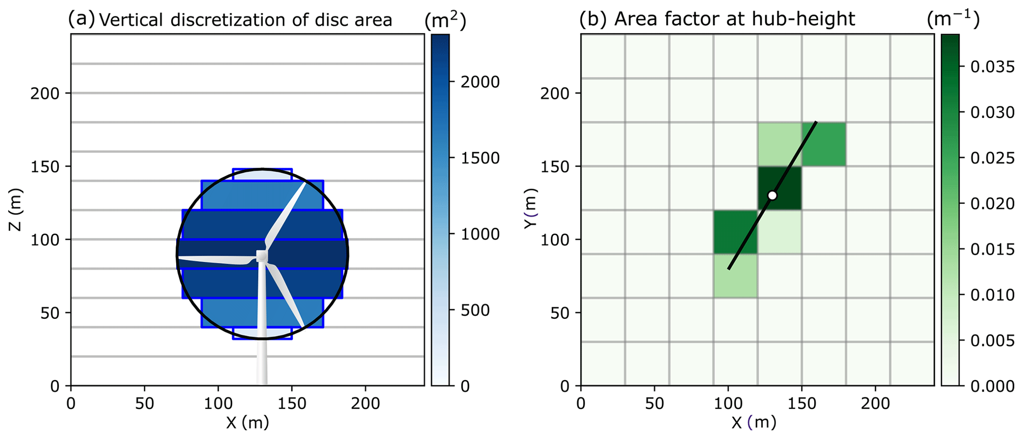
Figure 1 The illustration demonstrates the discretization of an actuator disk. (a) Vertically, the disk is divided into sections between each full vertical level. (b) The discretized area factor at the hub-height level is depicted. The actuation disk radius is 116 m, and the horizontal and vertical grid sizes are 30 and 20 m, respectively.

Normally, the unperturbed wind V₀ is unknown but related to the wind speed at the rotor, V, by

$$\begin{array}{}\text{(4)}& {\mathit{V}}_{\mathrm{0}}={\displaystyle \frac{\mathrm{1}}{\mathrm{1}-a}}\mathit{V},\end{array}$$

where a is the axial induction factor. We note that in the WRF model, the tendency terms are defined for the coupled velocity, which is defined as U=μ_du, with μ_d being the dry mass of the air column. Thus the tendency terms to be added to the model become

$$\begin{array}{}\text{(5)}& {\displaystyle }{\left.{\displaystyle \frac{\partial U}{\partial t}}\right|}_T=-{\displaystyle \frac{\mathrm{1}}{\mathrm{2}(\mathrm{1}-a{)}^{\mathrm{2}}}}{\mathit{\mu }}_{\mathrm{d}}{C}_{\mathrm{T}}\left|\mathit{V}\right|u{F}_{\mathrm{A}},\text{(6)}& {\displaystyle }{\left.{\displaystyle \frac{\partial V}{\partial t}}\right|}_T=-{\displaystyle \frac{\mathrm{1}}{\mathrm{2}(\mathrm{1}-a{)}^{\mathrm{2}}}}{\mathit{\mu }}_{\mathrm{d}}{C}_{\mathrm{T}}\left|\mathit{V}\right|v{F}_{\mathrm{A}}.\end{array}$$

The turbulence in the wake behind a wind turbine primarily arises from shear due to reduced wind speed in the wake region (Crespo and Herna, 1996; Quarton and Ainslie, 1990). In mesoscale modeling, incorporating turbulence kinetic energy (TKE) into wind farm parameterization is necessary due to the model's inability to resolve wakes at small scales (Fitch et al., 2012). Fitch et al. (2012) assumes that a portion of the extracted energy from the mean wind becomes power (related to power coefficient C_P), while the remainder becomes TKE, proportional to C_T−C_P. Given WRF-SADLES's target resolution of a few dozen meters, where the wake is partially resolved, some added subgrid-scale TKE may be necessary. Nevertheless, we tested the method used by Fitch et al. (2012), incorporating a source of subgrid-scale TKE as

$$\begin{array}{}\text{(7)}& {\left.{\displaystyle \frac{\partial {\mathrm{TKE}}_{\mathrm{sgs}}}{\partial t}}\right|}_T={\displaystyle \frac{\mathrm{1}}{\mathrm{2}(\mathrm{1}-a{)}^{\mathrm{3}}}}{\mathit{\mu }}_{\mathrm{d}}{C}_{\mathrm{TKE}}|\mathit{V}{|}^{\mathrm{3}}{F}_{\mathrm{A}},\end{array}$$

where $C_{\mathrm{TKE}}=f_{\mathrm{TKE}}(C_{\mathrm{T}}-C_{\mathrm{P}})$, where f_TKE is a factor that controls the amount of kinetic energy loss converted to TKE.

The tendency terms above depend critically on the axial induction factor a. Some previous studies have used certain specific values of a, such as $a=\mathrm{1}/\mathrm{4}$ (Calaf et al., 2010) or even a=0 (Fitch et al., 2012) (i.e., they used the wind speed at the grid point directly instead of the unperturbed wind speed). In our implemented SADLES model, we provide two options for estimating a:

• Option 1 (direct evaluation). First, the hub-height ambient wind speed $\left|{\mathit{V}}_{\mathrm{0}}\right|$ is evaluated at 2 rotor diameters (2 D) in front of the turbine. Then, the induction factor is calculated by

  $$a=\mathrm{1}-{\displaystyle \frac{\left|\mathit{V}\right|}{\left|{\mathit{V}}_{\mathrm{0}}\right|}}.$$

• Option 2 (inferred evaluation). In this option, only the hub-height wind speed at the rotor location is needed. Instead, we assume one-dimensional momentum theory ($C_{\mathrm{T}}=\mathrm{4}a(\mathrm{1}-a)$) and therefore

  $$a={\displaystyle \frac{\mathrm{1}}{\mathrm{2}}}(\mathrm{1}-\sqrt{\mathrm{1}-C_{\mathrm{T}}\left(\right|\mathit{V}\left|\right)}).$$

  Note that although the thrust curve is typically provided as a relation between C_T and the ambient wind speed $\left|{\mathit{V}}_{\mathrm{0}}\right|$, we can also establish the relation between C_T and the wind speed at the rotor $\left|\mathit{V}\right|$ using one-dimensional momentum theory.

In general, the direct evaluation of a (Option 1) is more intuitive. However, this method has some potential problems, including the formula being affected by the blockage effect, where the wind speed in front of the wind turbine is reduced. By using this formula, a can exceed 0.5, implying that the wind behind the turbine becomes opposite to the ambient wind. This is nonphysical and can lead to model instability. Thus, the upper limit of a is set to its inferred evaluated value (Option 2).

2.2 Cell perturbation

Traditional LESs often use periodic lateral boundary conditions, allowing turbulent eddies to fully develop and reach a quasi-steady state. However, nested downscaling approaches face limitations due to the restricted time and space within the inner domain. This restricted environment can hinder the complete development of eddies, particularly in scenarios with small domain sizes, high ambient wind speeds, or stable boundary layer conditions. These limitations can lead to slow turbulence development within the nested domain, impacting the accuracy of simulations.

The above problem can be alleviated using the cell perturbation method (Muñoz-Esparza et al., 2014, 2015), which is a simple and effective way to accelerate the development of turbulence within the nested domain. The method introduces a random perturbation of potential temperature within the interval of −0.5 to 0.5 K to three cells near the inflow boundaries. Each cell is an 8×8 grid point square in the horizontal plane, and the same perturbation is applied to each cell. Therefore, the total perturbation zone extends 24 grid points from the inflow boundaries.

In the idealized setup of Muñoz-Esparza et al. (2014), perturbations are introduced at every vertical grid point up to two-thirds of the inversion layer, which is known in the idealized setting. In our approach, the perturbations are applied with full magnitude up to a pre-defined vertical-level k₁ and then gradually reduced to 0 at a higher-level k₂ using the weight ${\cos }^{\mathrm{2}}\left[\mathrm{0.5}\mathit{\pi }(k-k_{\mathrm{1}})/(k_{\mathrm{2}}-k_{\mathrm{1}})\right]$, where k is the vertical level. As noted by Muñoz-Esparza et al. (2014), the perturbation process should not be done at every time step but at an interval that is at least equal to the perturbation timescale, $T_{\mathrm{s}}=\mathrm{8}\mathrm{\Delta }x/U$, where U is the characteristic velocity scale, and Δx is the horizontal grid spacing.

Because the cell perturbation method is not available with the distribution of WRF, we included our implementation within the distribution of WRF-SADLES.

2.3 Code implementation and turbine information

We have integrated the SADLES code into the Advanced Research WRF (ARW), version 4.3.1, with MPI support. This was achieved by adding two new Fortran 90 modules: a SADLES module (module_sadles.F) and a cell perturbation module (module_cellpert.F), which both serve as the WRF's physics package (located in the phys directory). The new namelist options for these modules were incorporated into the WRF model by modifying the WRF's registry. During the first step of the Runge–Kutta loop (within module_first_rk_step_part1.F), tendency terms of the SADLES module are added to the model, while the potential temperature perturbation from the cell perturbation is incorporated after the integration loop (within solve_em.F). Tables A1 and A2 outline the available options in the SADLES and cell perturbation modules. This modified WRF system also enables the simulation of turbine behavior in idealized experiments, with additional namelist options for specifying the Coriolis parameter and surface roughness length. The code has been released as open source to foster open research (Bui, 2023b), with the aspiration of its inclusion in the official WRF repository. Users can implement WRF-SADLES by copying these modules and overriding a few related files within the existing WRF file structure, followed by recompiling the model system. In the subsequent section, we utilize turbine data from Larsén and Fischereit (2021), which provide the locations, thrust curves, and power curves of wind turbines from various wind farms in the North Sea.

3 Idealized simulation

3.1 Experiment design

To start, we investigate the calculation of the axial induction factor (e.g., Option 1 or Option 2) and the additional tendency for sub-grid TKE (i.e., f_TKE). Due to challenges in acquiring relevant observational data, we conducted and compared idealized experiments employing a single 5 MW turbine using the WRF-SADLES and PALM models. Simulations were executed at two resolutions: 10 m (high resolution, about 12 grid points per rotor diameter) and 30 m (target intermediate resolution, about 4 grid points per rotor diameter).

Table 1 summarizes the experiments conducted using the WRF-SADLES and PALM models. For the WRF-SADLES simulations, experiments with suffixes _Opt1 and _Opt2 represent different options for calculating the axial induction factor a, with Option 1 employing direct evaluation and Option 2 employing inferred evaluation. In these experiments, f_TKE takes the default value of 0.5. Additionally, experiments with suffixes _TK0 and _TKE1, both utilizing Option 2, aim to investigate the effect of adding TKE tendency as in Eq. (7), with f_TKE set to 0 and 1, respectively.

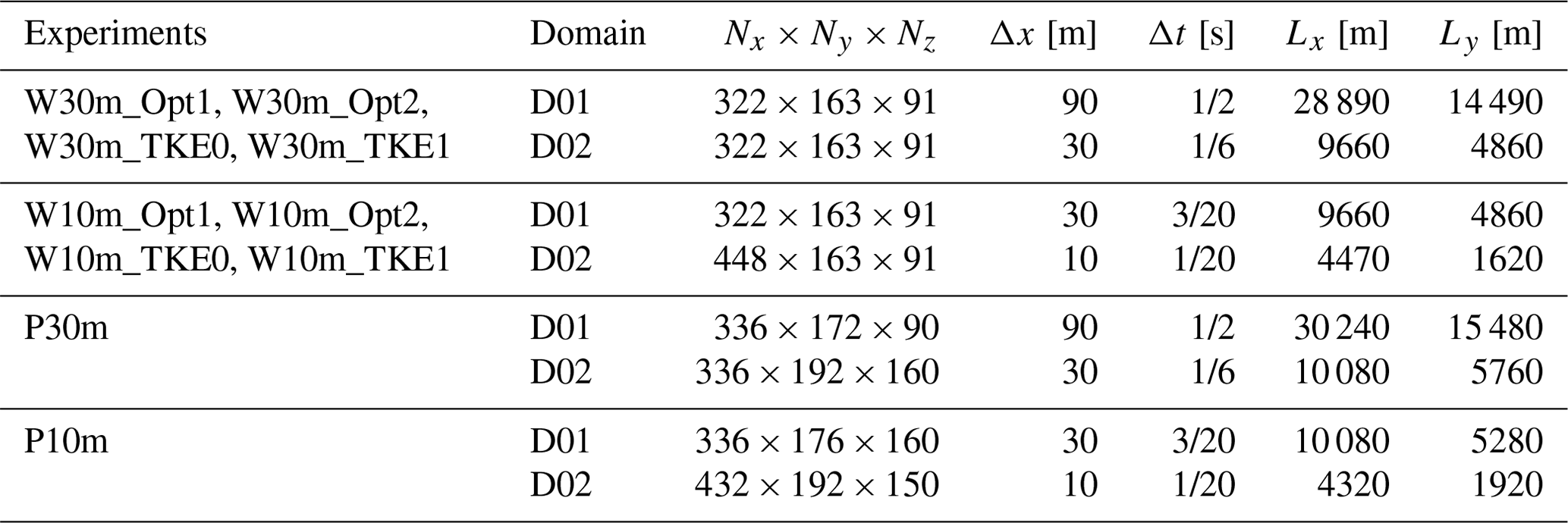
Table 1 Domain configurations for the idealized WRF (prefix W) and PALM (prefix P) experiments.

WRF-SADLES configurations

The domain configurations for each experiment are summarized in Table 1. Each experiment utilized two nested domains (D01 and D02), with the outer domain D01 having a coarser resolution (30 or 90 m) and using periodic boundary conditions on all sides, and the inner domain D02 (10 or 30 m) applying cell perturbation at the inflow boundary on the west side. All domains except the 10 m domain had a horizontal aspect ratio of 2:1. The 10 m domain had a longer aspect ratio of 2.76:1 to allow the turbulence and turbine wake to evolve over a longer distance.

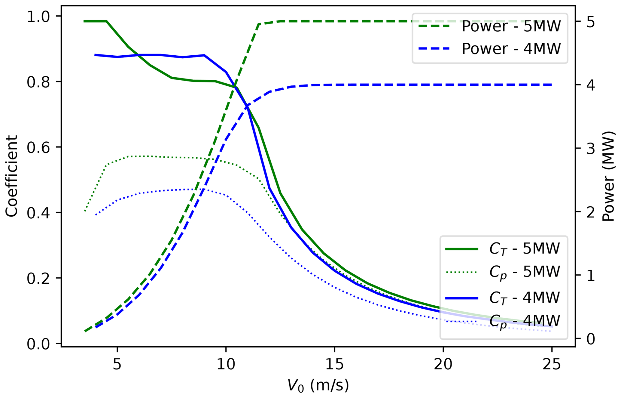
Figure 2 Thrust coefficient (C_T), power coefficient (C_P), and turbine power as functions of ambient wind speed (V₀) are shown for the 4 and 5 MW wind turbines used in the idealized (5 MW) and realistic (4 and 5 MW) experiments in this paper.

The top model level for all experiments is set at 1600 m, with an 800 m Rayleigh damping layer at the top with a coefficient of 0.2 s⁻¹. There is no vertical level stretching for the 30 m resolution experiments. In the case of the 10 m experiments, the vertical levels are stretched such that the near-surface vertical resolution is roughly 10 m. The initial potential temperature is 288 K from the surface up to 500 m and then increases with a lapse rate of 1 K per 100 m.

Our idealized simulations employed the revised MM5 Monin–Obukhov surface layer scheme (Jiménez et al., 2012) with a surface roughness length of 1 mm. We enabled LES mode by deactivating the boundary layer parameterization scheme. Instead, the 1.5-order three-dimensional TKE closure was used (Lilly, 1967), treating the subgrid-scale TKE as a prognostic variable. The Coriolis parameter was set to $\mathrm{1.177}\times {\mathrm{10}}^{-\mathrm{4}}$ s⁻¹, corresponding to a 54° N latitude.

In idealized LES, the focus is on resolving the turbulent structures within the domain. To achieve this, non-essential physical parameterization schemes, including microphysics, cumulus convection, and radiation, were disabled. The effect of surface radiation on the development of turbulence is represented by a surface turbulence heat flux of $\stackrel{\mathrm{‾}}{({\mathit{\theta }}^{\prime }{w}^{\prime }{)}_{\mathrm{s}}}=\mathrm{0.02}$ K m s⁻¹, similar to some previous studies (Muñoz-Esparza et al., 2014; Kale et al., 2022). This presents a weak convective boundary layer.

At the center of the inner domain, we placed a 5 MW wind turbine used at the Alpha Ventus wind farm. The turbine information taken from Larsén and Fischereit (2021) includes a rotor diameter of 116 m, a hub height of 90 m, and the thrust and power curves at different wind speeds (Fig. 2).

To achieve a quasi-equilibrium state of turbulence, a specialized LES model such as PALM typically conducts a precursor run, often using a smaller domain to minimize computational costs. However, this precursor technique is not supported within the WRF model. Instead, we opt for a spin-up period of 20 h solely in the outer domain. To align the wind within the boundary layer predominantly in the zonal (eastward) direction, we adjust the geostrophic wind to rotate slightly to the left, specifically setting U_g=10.24 m s⁻¹ and $V_{\mathrm{g}}=-\mathrm{1.39}$ m s⁻¹. Following the spin-up period, both domains are simulated for 4 h, with a 1 min output interval for the inner domain (D02) to facilitate further analysis.

PALM configurations

To evaluate the performance of the SADLES module in simulating turbine wakes, we compared the results from the WRF-SADLES model with those from the PALM model (Maronga et al., 2015, 2020) system 21.10 revision r4901. PALM is an LES model developed at Leibniz Universität, Hanover, Germany, and has been shown in several studies to be capable of simulating wind turbine wakes effectively (e.g., Witha et al., 2014; Vollmer et al., 2015; Dörenkämper et al., 2015).

In PALM, the wind turbine is represented by an advanced AD+R model that is based on the BE method (Dörenkämper et al., 2015), which calculates both the thrust force and the torque force as functions of radius and tangential angle from the center of the rotor. Similar to the GAD methods (Mirocha et al., 2014; Kale et al., 2022), the wind turbine model in PALM computes the local lift and drag forces and requires additional information on the turbine and blade aerodynamic properties. For this reason, currently only three types of wind turbines are officially supported, including the National Renewable Energy Laboratory (NREL) 2.3, 5, and 15 MW models (Jonkman et al., 2009; Gaertner et al., 2020; Ardillon et al., 2023). To compare with WRF-SADLES, we used the NREL 5 MW model with the same hub height of 90 m. However, the rotor diameter of the NREL 5 MW is slightly larger at 128 m compared to the 116 m diameter of the 5 MW turbine used in WRF-SADLES.

The two idealized experiments, P10m and P30m, have two nested domains similar to the WRF-SADLES experiments (see Table 1 for domain configurations). Cyclic lateral boundary conditions were used for the coarser domain. To prepare initial conditions for the main run, we used a precursor run for 24 h to reach a quasi-steady-state condition. Compared to the simulation domain, the precursor domain has the same number of vertical levels but only has 96×64 horizontal grid points to reduce the computational cost.

To parameterize subgrid-scale turbulence in PALM, we used 1.5-order closure (Deardorff, 1980; Moeng and Wyngaard, 1988; Saiki et al., 2000). We initialized atmospheric conditions similar to those in the WRF-SADLES experiments, including an initial potential temperature of 288 K, and a geostrophic wind of approximately 10 m s⁻¹ from the west. Similar to WRF-SADLES, in idealized simulations of PALM, we do not use other physics parameterizations, such as microphysics, cumulus, and radiation. Although for some LES applications of urban conditions, the solar radiation processes may play an important role (e.g., Salim et al., 2020; Krč et al., 2021), in typical LES with a flat surface like ours, the radiation parameterization is not used to focus on the main responsible processes and reduce computation (Avissar and Schmidt, 1998). The effect of solar radiation is instead represented by a uniform surface turbulence heat flux of $\stackrel{\mathrm{‾}}{({\mathit{\theta }}^{\prime }{w}^{\prime }{)}_{\mathrm{s}}}=\mathrm{0.02}$ Wm s⁻², similar to WRF-SADLES's idealized simulations.

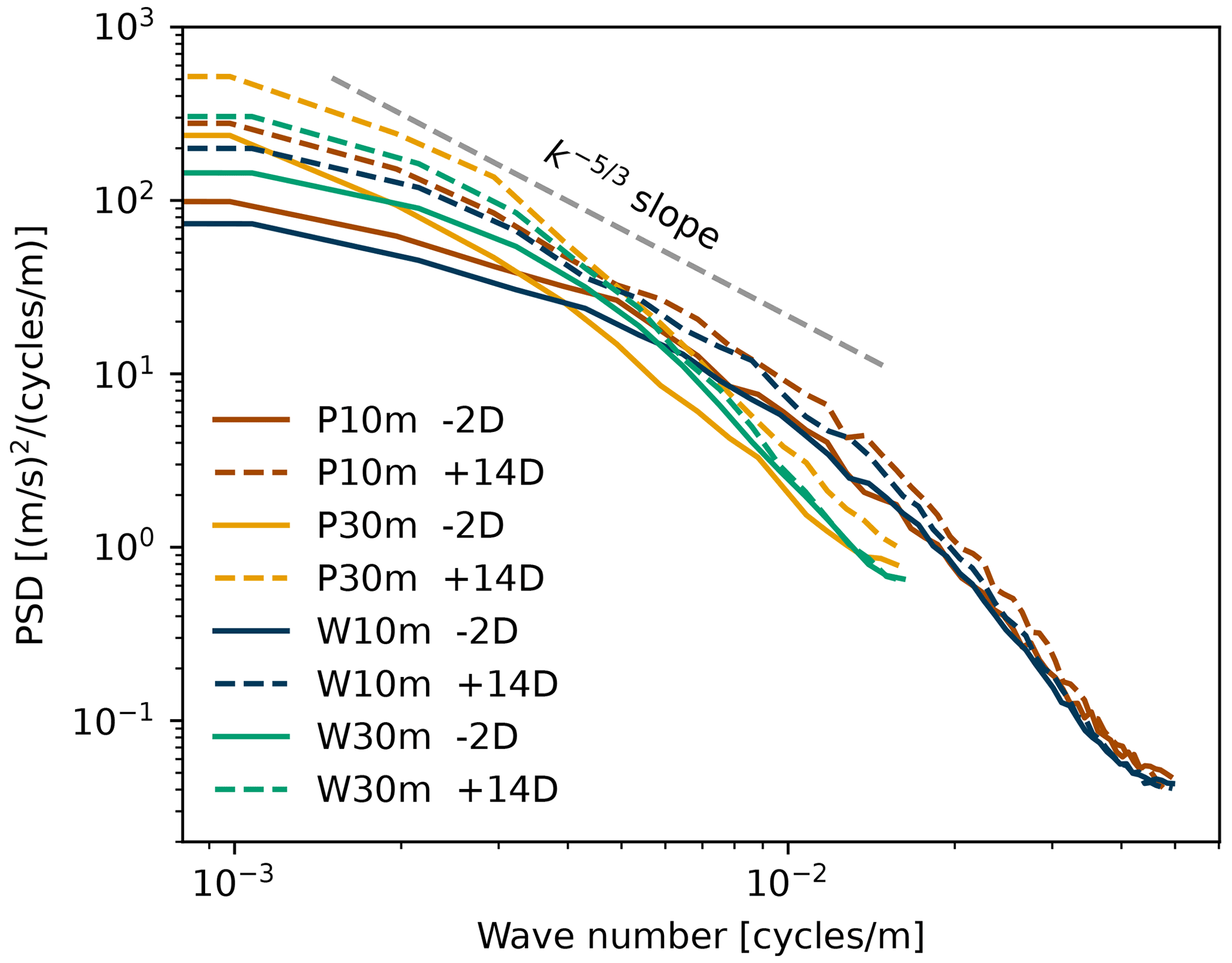
Figure 3 Time-averaged power spectral densities (PSDs) of wind speed spatial fluctuations for the PALM (P10m, P30m) and WRF-SADLES (W10m, W30m) simulations at two locations: −2 D upstream and +14 D downstream of the wind turbine. The analysis was computed from a meridional (south–north direction) line at hub height with a length of 8 D centered on the wake center. To improve clarity and avoid redundancy, we present the average results of all WRF-SADLES simulations at each resolution (W30m and W10m for 30 and 10 m resolutions, respectively).

3.2 Result

We first examine the turbulence characteristic of WRF-SADLES and PALM at different resolutions by carrying out wavenumber spectrum analysis for a meridional (south–north) cross-section at hub height with a length of 8 D, centered on the wake axis (Fig. 3). Both WRF-SADLES and PALM simulations exhibit similar trends in turbulence properties. Simulations with a 10 m resolution capture higher turbulence levels for smaller-scale structures (wavenumbers $>\mathrm{4}\times {\mathrm{10}}^{-\mathrm{3}}$ cycles m⁻¹, corresponding to wavelengths shorter than 250 m). This indicates a better ability to resolve these structures with finer resolution. This suggests limitations in capturing the energy transfer mechanisms at these scales. Compared to the 30 m resolution, the 10 m resolution exhibits a broader range of applicability for the Kolmogorov power law, spanning approximately $\mathrm{2}\times {\mathrm{10}}^{-\mathrm{3}}$ to 10⁻³ cycles m⁻¹ (corresponding to wavelengths between 100 and 500 m). This wider range signifies a more accurate representation of the energy cascade across different scales in these simulations. Furthermore, all simulations show an increase in turbulence energy at the far-wake distance (14 D) compared to upstream turbulence (−2 D), for all wavenumbers, indicating that the turbine has an effect of increasing the turbulence behind it. This behavior is consistent for both PALM and WRF-SADLES models.

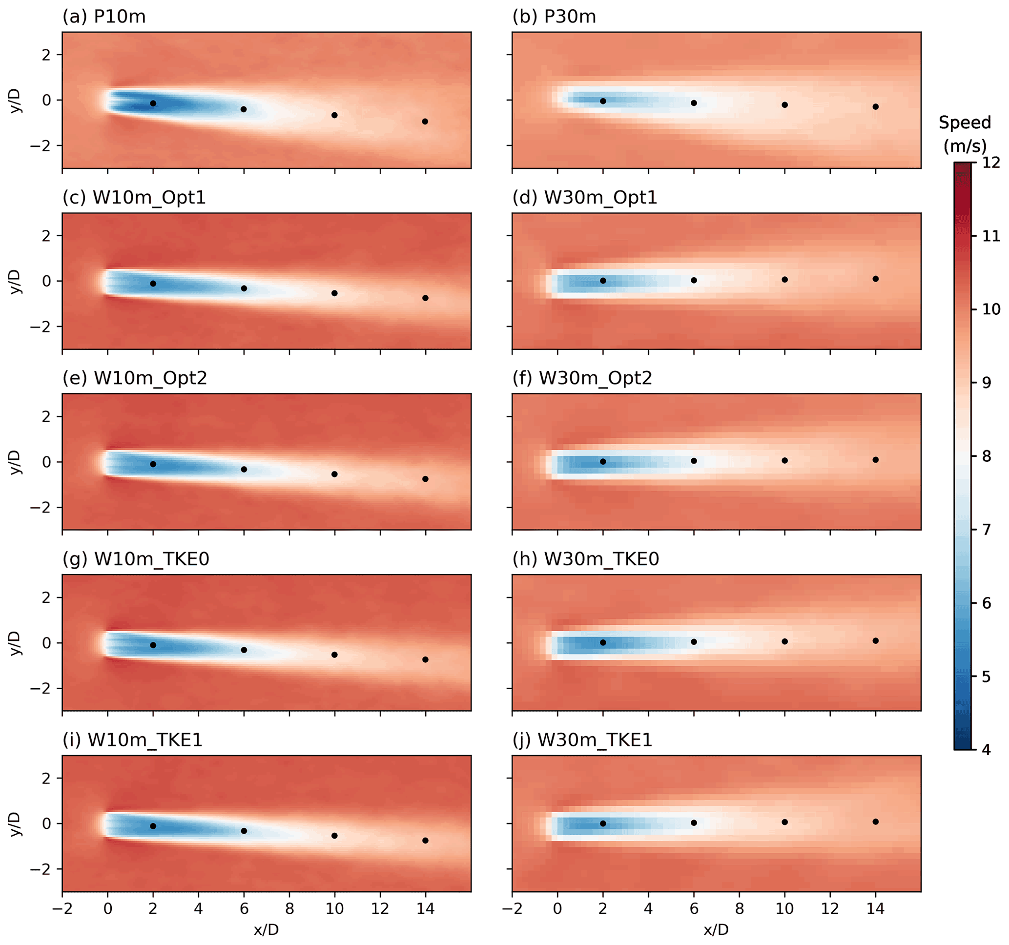
Figure 4 The 4 h average wind speeds at the turbine hub height (90 m) for PALM (a, b) and WRF-SADLES (c–j) simulations with different resolutions and options for axial induction factors and f_TKE values (=0 for _TKE0, =1 for _TKE1). The black dots indicate distances of 2, 6, 10, and 14 D behind the turbine.

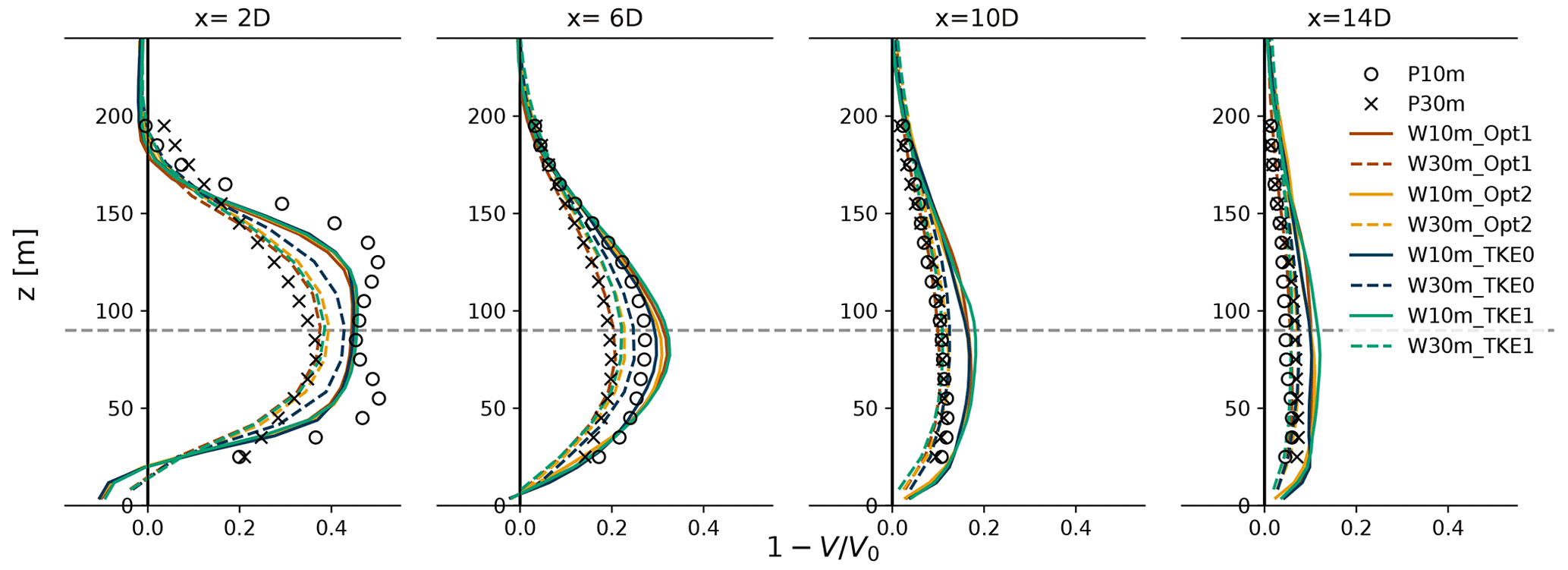
Figure 5 Vertical profile of wake deficit ($\mathrm{1}-V/V_{\mathrm{0}}$) for idealized experiments at distances behind the turbine of 2, 6, 10, and 14 D. The evaluation locations are indicated by the black dots in Fig. 4.

Figure 4 shows the average wind speeds over 4 h for the PALM and WRF-SADLES idealized experiments. For both PALM and WRF-SADLES, the differences between 10 and 30 m resolution are more noticeable than the difference between the two models and between different options of WRF-SADLES. Vertically, the 10 m resolution PALM exhibits two maximums above and below the hub height at the near-wake distance (Fig. 5, x=2 D), which results from the BE method. This feature is not present in the 30 m PALM simulation and the WRF-SADLES experiments. For further distances downstream, there is a similarity in the shape of the wake deficit for 10 and 30 m for both models, with one single maximum slightly below the hub height (Fig. 5, $x=\mathrm{6},\mathrm{10},\mathrm{14}D$).

Both PALM and WRF-SADLES simulations have a stronger wake deficit for higher resolution for distances shorter than 6 D (Fig. 5). For longer distances, the wake deficit of 10 m PALM eventually becomes weaker than 30 m, indicating a faster wake recovery and stronger turbulence activity for the higher resolution. On the contrary, the wake deficit of 10 m WRF-SADLES at a longer distance of 14 D is still significantly stronger than the 10 m simulation, indicating a slower wake recovery. Visibly, the 10 m WRF-SADLES simulations exhibit weaker wake expansion than the 30 m WRF-SADLES simulation, which is more in agreement with the 10 m PALM simulation (Fig. 4).

Minimal differences are observed for the two methods calculating the axial induction factor in WRF-SADLES (Figs. 4 and 5). This validates the one-dimensional momentum theory of the actuator disk for calculating the axial induction factor a. Given that Option 1 necessitates wind speed evaluation in front of the turbine, it may be sensitive to model resolution and blockage effects. Therefore, we recommend the use of Option 2 in practical applications. Additionally, being derived from the one-dimensional momentum theory, Option 2 is also consistent with the simple actuator disk method of WRF-SADLES.

Compared to the two axial induction factor calculation methods within WRF-SADLES, the effects of subgrid-scale TKE are more pronounced on wake development (Fig. 5, at 2 and 6 D). Using the 10 m PALM simulation as a reference, the WRF simulation without added TKE (f_TKE=0) exhibits the best agreement in terms of wake deficit for both 10 and 30 m resolutions at all distances. At distances exceeding 10 D, the 30 m WRF-SADLES simulation gets even closer to the reference than the 10 m WRF-SADLES. Interestingly, at the 10 m resolution, WRF-SADLES with added TKE (W10m_TKE1) shows a slightly slower wake recovery compared to the experiment without added TKE (W10m_TKE0), as evidenced by a stronger wake deficit at 10 and 14 D in Fig. 5.

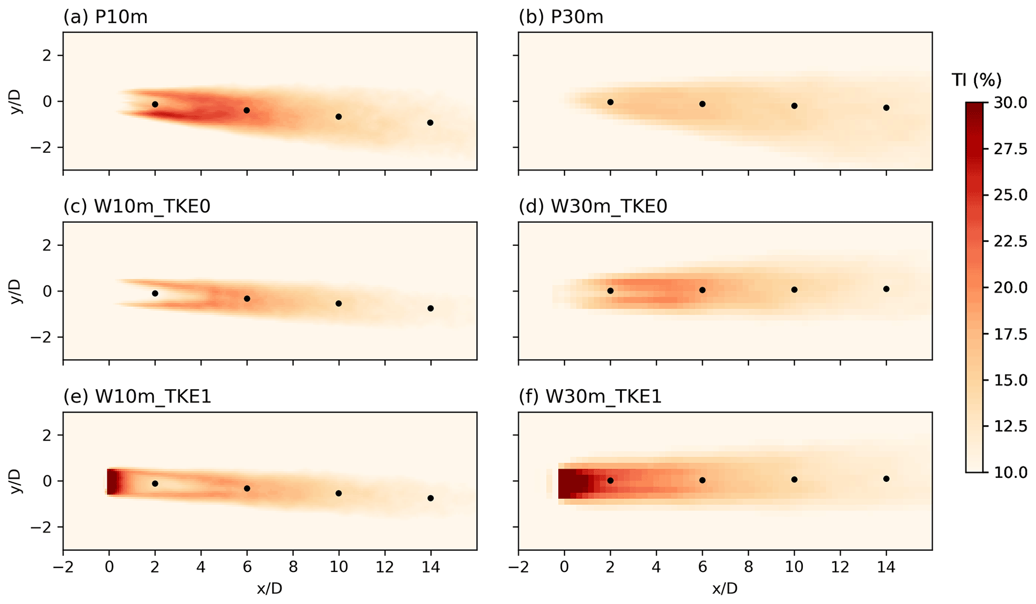
Figure 6 The 4 h turbulence intensity ($\stackrel{\mathrm{‾}}{\mathrm{TI}}$) at hub height (90 m) for PALM (a, b) and WRF-SADLES (c–f) simulations with (_TKE1) or without added TKE (_TKE0) and different resolutions of 10 and 30 m. The black dots indicate distances of 2, 6, 10, and 14 D behind the turbine.

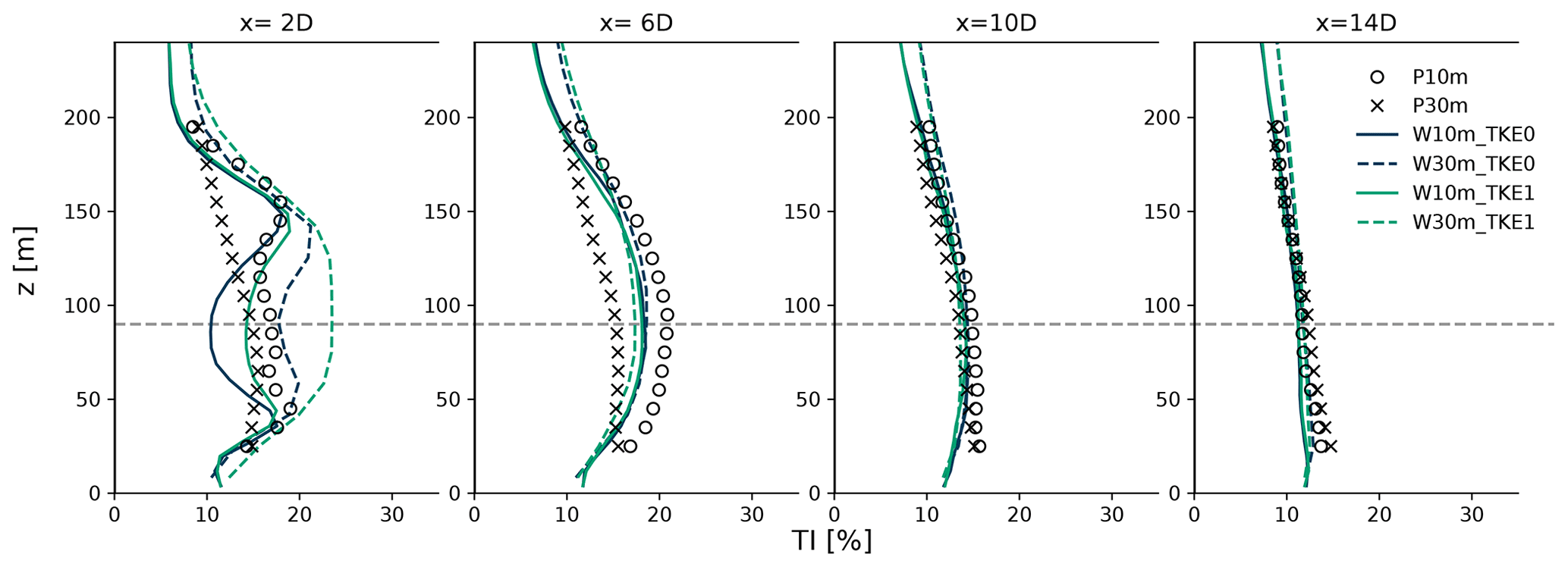
Figure 7 Vertical profile of the time-averaged turbulence intensity $\stackrel{\mathrm{‾}}{\mathrm{TI}}$ for PALM and WRF-SADLES simulations with (_TKE1) or without added TKE (_TKE0) at distances behind the turbine of 2, 6, 10, and 14 D. The evaluation locations are indicated by the black dots in Fig. 4.

To investigate why the added subgrid-scale TKE source has minimal impact on the wake development in WRF-SADLES and even exhibits a negative impact on wake recovery at the 10 m resolution, we compared the calculated average turbulence intensity (TI) between the experiments. The average TI is computed using the following equation:

$$\begin{array}{}\text{(8)}& \stackrel{\mathrm{‾}}{\mathrm{TI}}={\displaystyle \frac{\sqrt{\frac{\mathrm{2}}{\mathrm{3}}\stackrel{\mathrm{‾}}{\mathrm{TKE}}}}{\left|\mathit{V}\right|}},\end{array}$$

where $\stackrel{\mathrm{‾}}{\mathrm{TKE}}$ represents the time-averaged total turbulence kinetic energy and is the sum of grid-scale (${\stackrel{\mathrm{‾}}{\mathrm{TKE}}}_{\mathrm{gs}}$) and subgrid-scale (${\stackrel{\mathrm{‾}}{\mathrm{TKE}}}_{\mathrm{sgs}}$) terms. ${\stackrel{\mathrm{‾}}{\mathrm{TKE}}}_{\mathrm{sgs}}$ is a prognostic variable derived from the 1.5-order turbulence closure within the PALM and WRF-SADLES models. On the other hand, the grid-scale term is derived from ${\stackrel{\mathrm{‾}}{\mathrm{TKE}}}_{\mathrm{gs}}=\frac{\mathrm{1}}{\mathrm{2}}(\stackrel{\mathrm{‾}}{{u^{\prime }}^{\mathrm{2}}}+\stackrel{\mathrm{‾}}{{v^{\prime }}^{\mathrm{2}}}+\stackrel{\mathrm{‾}}{{w^{\prime }}^{\mathrm{2}}})$, where u^′, v^′, and w^′ denote the deviations of wind speed components from their respective time averages over the simulation period.

All experiments show a consistent TI of around 10 % outside the wake regions (Figs. 6 and 7). Both PALM and WRF-SADLES simulations exhibit TI development at the edges of the wake regions due to the increased wind shear at these boundaries (Fig. 6). Without added TKE, the TI at the turbine location is equal to its the environmental value. When the subgrid-scale TKE is added (_TKE1), the TI has a maximum TI exceeding 30 % at the turbine location (Fig. 6e, f). Significant discrepancies in the TI profiles are observed only in the vertical profiles of TI between the two models (PALM and WRF-SADLES) and resolutions (10 and 30 m) at the near-wake distance (Fig. 7, x=2 D). The experiments with 10 m resolution show two TI peaks above and below the hub height, likely due to the turbulence production associated with the wake shear. These peaks reach a TI of about 20 % and are consistent between the PALM and WRF-SADLES models.

However, this added subgrid-scale TKE primarily impacts the near-wake region and has minimal effect further downstream (Fig. 7, $x=\mathrm{6},\mathrm{10},\mathrm{14}D$) as the TI quickly dissipates as it advects downstream. The TI levels for WRF-SADLES without added TKE show even better agreement with the reference experiment for both resolutions (30 and 10 m). These findings challenge the underlying assumption of Fitch et al. (2012), as the TKE downstream should relate to wake deficit, which is linked to C_T and not to C_T−C_P. In an idealized scenario where all TKE extracted from the mean wind converts to power (C_T=C_P), according to Fitch, no TKE is generated, which is not appropriate. Thus, we propose that mesoscale WFPs should consider the relationship between added turbulence and C_T, alongside factors like stability conditions. Therefore, we recommend using the WRF-SADLES model without the added subgrid-scale TKE source (i.e., f_TKE=0) in practical applications.

4 Meso-to-micro realistic downscaling simulation

This section demonstrates meso-to-micro downscaling using global reanalysis data. We employ the ERA5 data set from the European Centre for Medium-Range Weather Forecasts (ECMWF) (Hersbach et al., 2020). These data have a spatial resolution of approximately 31 km and are available hourly. First, we briefly compare the simulation results with observational data from the FINO1 meteorological station in the southern North Sea. This comparison aims to assess the model's ability to reproduce real-world conditions. Subsequently, we provide an example illustrating power loss due to farm-to-farm interaction.

4.1 Model configurations

To achieve turbine-scale resolution, we employed a system of five nested domains (detailed in Table 2). Each domain progressively reduces its grid size for finer resolution. The first three domains (D01, D02, D03; see Fig. 8a) focus on downscaling the mesoscale processes, while the final two domains (D04, D05; see Fig. 8b) transition to large-eddy simulation (LES) for high-resolution wind flow near the turbines.

The outermost domain (D01) has a resolution of 9 km, encompassing a vast region that includes Europe and the northeastern Atlantic Ocean (Fig. 8a). The second domain (D02) zooms in on the North Sea (Fig. 8a). The remaining three domains are centered around the Alpha Ventus wind farm, located near the FINO1 meteorological mast station (Fig. 8b).

The first LES domain (D04) has a resolution of 200 m and acts as an intermediate step between the mesoscale and turbine-scale domains. It does not include wind turbines within its simulation. The innermost domain (D05) has the highest resolution of 40 m and encompasses a smaller area (19.2 km × 19.2 km) compared to a single grid cell of the original ERA5 data. This is the domain where the SADLES model is activated to simulate turbine wakes.

In domain D05, four wind farms comprising 5 and 4 MW turbines are present. Notably, the Alpha Ventus wind farm, featuring 12 turbines, is situated to the right of the FINO1 mast station. Detailed turbine specifications, including power and thrust curves, can be found in Larsén and Fischereit (2021) (refer to Fig. 2). For the subsequent experiments, we adopted SADLES Option 2 for the inferred evaluation of the axial induction factor, along with the f_TKE value of 0.

For vertical grid resolution, we adopted 60 levels following Bui and Bakhoday-Paskyabi (2022). This setup provides high resolution near the surface, approximately 10 m, with 21 levels below 500 m height. Regarding physical parameterization, we employed the following options: the rapid radiative transfer model for general circulation models (RRTMG) scheme (Iacono et al., 2008) for radiation parameterization across all domains and the Thompson graupel scheme (Thompson et al., 2008) for microphysics parameterization. The Tiedtke scheme (Zhang et al., 2011) was utilized for cumulus parameterization in the outermost 9 km domain (D01), with cumulus parameterization disabled in finer-resolution domains. For surface layer parameterization, we utilized the Monin–Obukhov similarity scheme (Jiménez et al., 2012), and the Noah land surface model (Mukul Tewari et al., 2004) was employed for land surface parameterization in all domains. The Yonsei University (YSU) scheme (Hong et al., 2006) was chosen for PBL parameterization in mesoscale domains (D01–D03), while PBL parameterization was disabled in LES domains (D04, D05). To simulate large eddies in LES domains, we employed the 1.5-order three-dimensional TKE closure (Lilly, 1967), supplemented by the cell perturbation method along the southern and western boundaries for the first 16 levels from the surface (up to approximately 300 m height) to initiate turbulence development.

Table 2 WRF domain configurations for the realistic downscaling experiments.

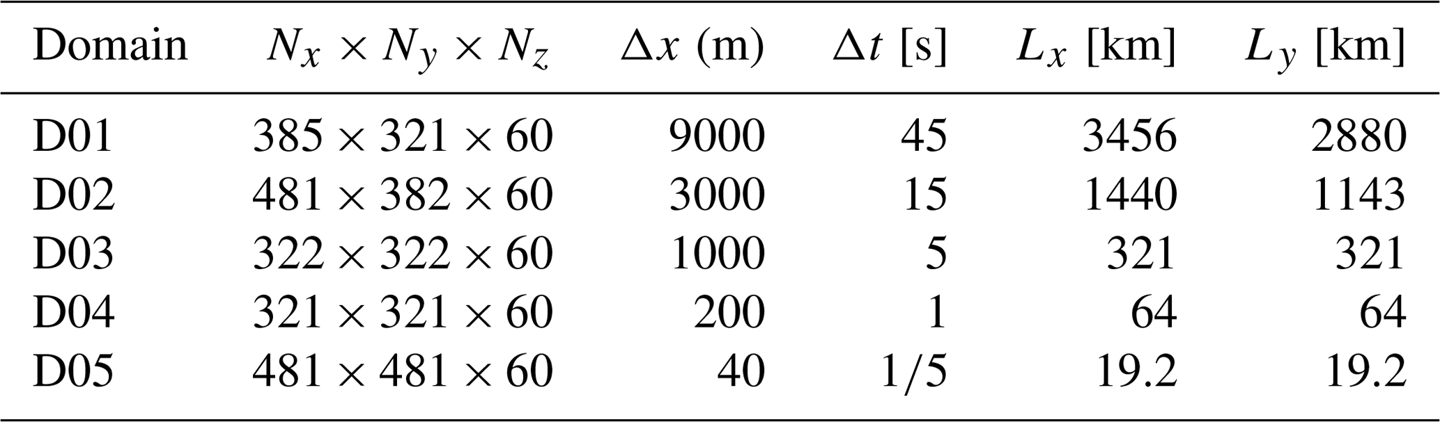
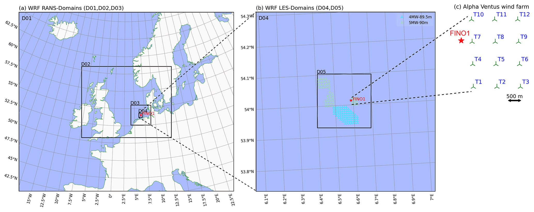
Figure 8 WRF domains used in the meso-to-micro downscaling simulations. The first three domains (a, D01–D03) are for mesoscale simulations, while the two innermost domains (b, D04, D05) are for LESs. The SADLES model is enabled in D05, with wind turbine locations marked by green and cyan markers. (c) Layout of the 12-turbine Alpha Ventus wind farm. The FINO1 meteorological mast station is indicated by the red star. Refer to Table 2 for detailed domain dimensions.

4.2 Comparison with observational data

This section briefly evaluates the performance of WRF-SADLES using observations from the FINO1 meteorological mast station. We compare wind speed and direction data collected by cup anemometers at 90 m (hereafter referred to as “mast data”) with WRF-SADLES simulations. Additionally, we utilize data from a Windcube © 100 s wind lidar (Kumer et al., 2014) (hereafter referred to as “lidar data”). The lidar data provide vertical profiles of wind speed and direction from vertical scans, along with line-of-sight (LOS) velocity from horizontal scans.

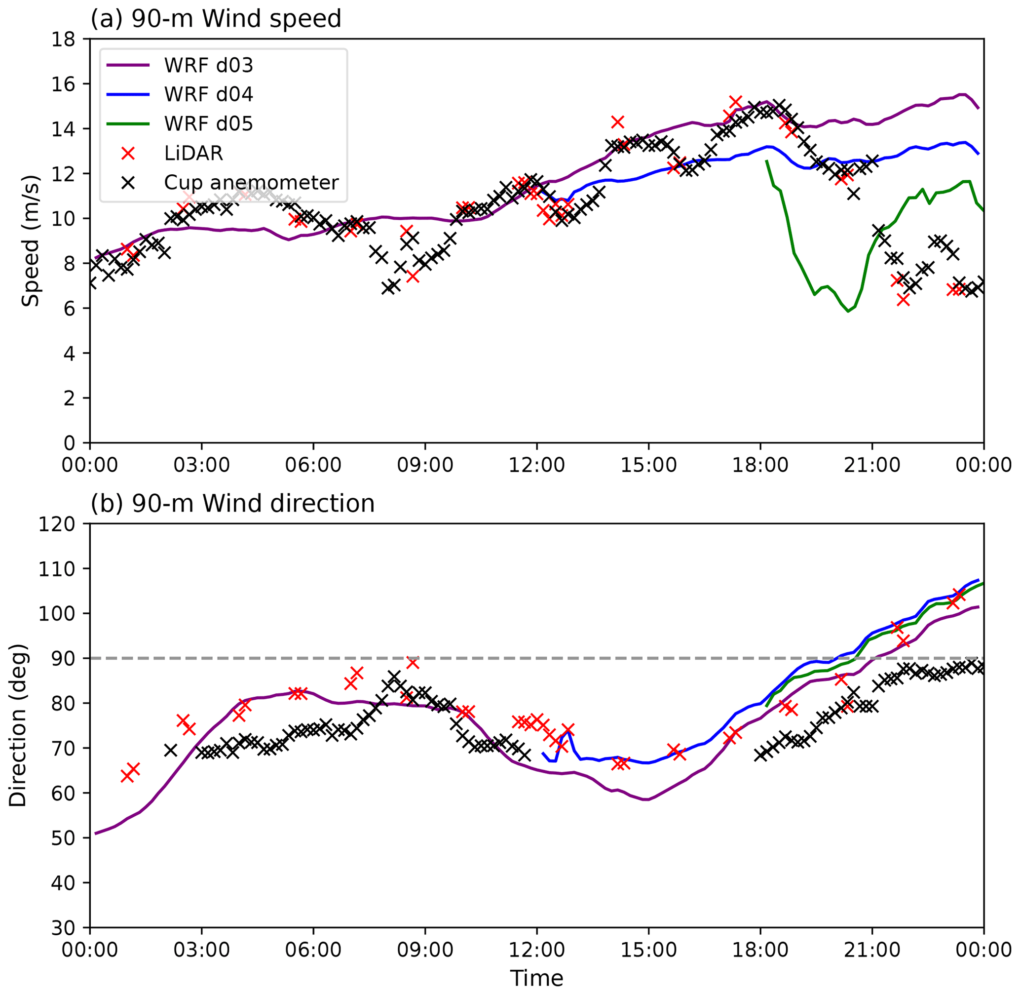
Figure 9 Time series of hub height wind speed (a) and wind direction (b) at the FINO1 met mast station on 13 August 2015, from 00:00 to 24:00 UTC, with data from WRF-meso (D01), WRF-LES (D02), WRF-SADLES (D03), lidar, and cup anemometers (mast).

The simulation period spans from 00:00 to 24:00 UTC on 12 August 2015. During this time frame, the first three domains (D01, D02, D03) run from 00:00 to establish mesoscale conditions, while the 200 m WRF-LES domain (D04) begins at 12:00 UTC to serve as an intermediary between meso- and microscales. Finally, the 40 m WRF-SADLES domain starts at 18:00 UTC to simulate turbine wakes. This period was selected because, towards its end, the wind direction shifts eastward, allowing for observation of wake effects using measurement data from the FINO1 station. Additionally, a low-level jet (LLJ), characterized by maximum wind speeds within the atmospheric boundary layer (ABL), is also observed during this time frame.

Figure 9 compares wind speed and wind direction at 90 m (hub height of the 5 MW Alpha Ventus wind turbines) from WRF simulations (D03: WRF-meso, D04: WRF-LES, and D05: WRF-SADLES) with observations from the FINO1 mast. Observations from both the mast data and the lidar data suggest the wake effect from nearby turbines partially reduces wind speeds around 09:00, 13:00, 17:00, and 19:00 UTC, with reductions of approximately 2 m s⁻¹. From 22:00 onwards, the wakes exhibit a full effect, particularly when the wind direction approaches easterly (90°), with wind speeds reduced from 6 to 8 m s⁻¹. While both data sources show good agreement in wind speed, there is a consistent difference of around 10° in wind direction between the mast data and lidar data.

After a few hours of spin-up time, WRF-meso wind speeds agree well with observations when wakes do not affect the location. However, the intermediate LES domain (D05) underestimates wind speeds by about 2 m s⁻¹. Without the inclusion of the wind turbine model, neither WRF-meso nor WRF-LES captures the wake effect at the FINO1 location. In contrast, WRF-SADLES, which includes a wind turbine model, successfully simulates the full wake effect at FINO1. Wind speeds are reduced to around 6 m s⁻¹, aligning well with observations. However, the timing of the wake impact differs, occurring between 19:00 and 21:00 UTC, roughly 2 h earlier than observed.

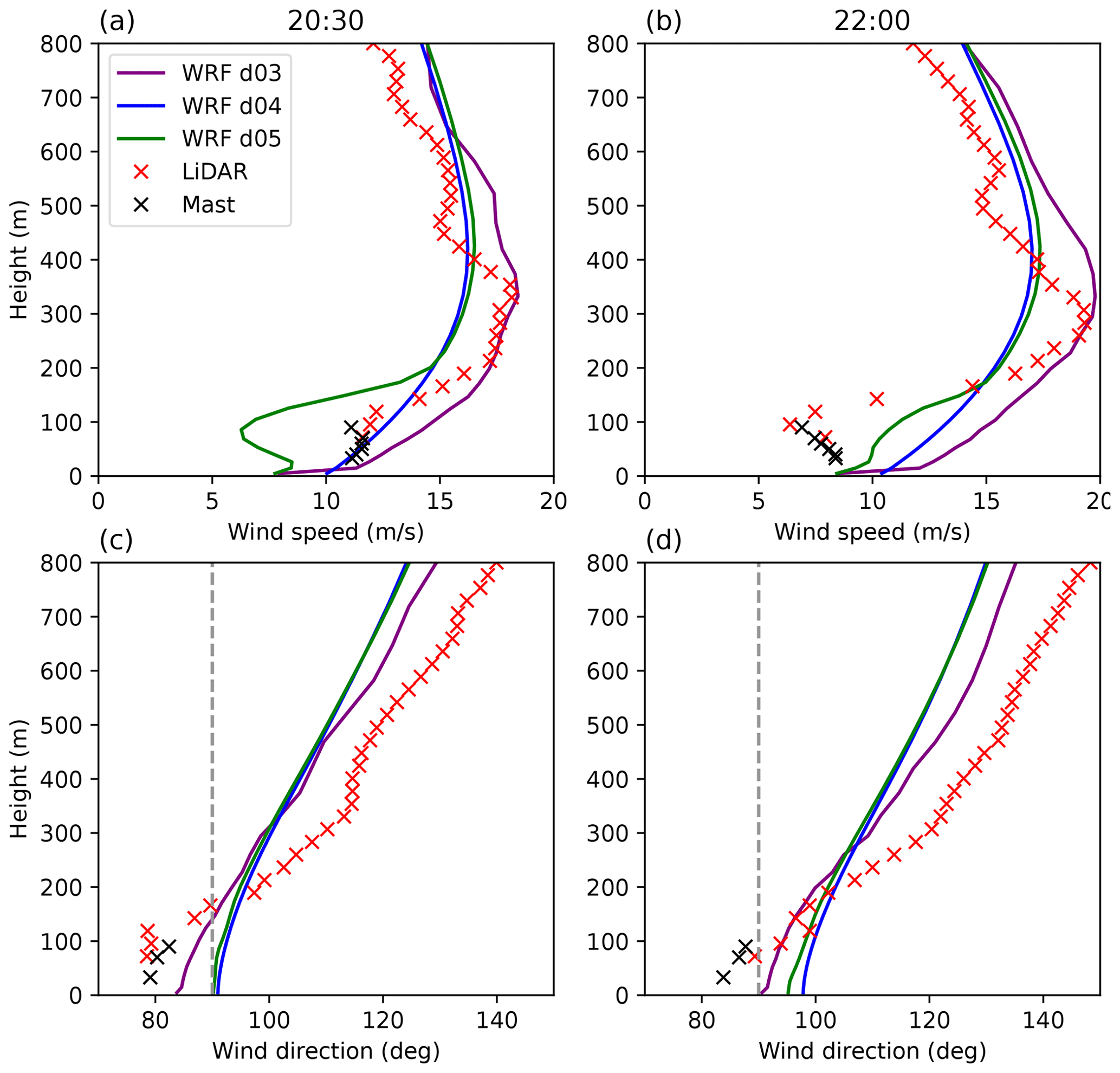
Figure 10 Vertical profiles of wind speed (a, b) and wind direction (c, d) recorded at the FINO1 met mast station on 13 August 2015, at 20:30 UTC (a, c) and 22:00 UTC (b, d), with data from WRF-meso (D01), WRF-LES (D02), WRF-SADLES (D03), lidar, and cup anemometers (mast).

To gain a clearer understanding of the discrepancies between WRF-SADLES simulations and observations, we examine the vertical profiles of wind speed (Fig. 10a) and wind direction (Fig. 10b) at two key points in time. The first is 20:30 UTC when the WRF-SADLES simulation shows the full wake effect. The second is 22:00 UTC when the full wake effect is observed in the data. At both times, the lidar data reveal an LLJ structure with a wind speed maximum of 17–20 m s⁻¹ at around 300 m. The observations of wind direction indicate wind veering, where the wind direction consistently turns clockwise with increasing height. However, within the overlapping region from 90 to 150 m, some discrepancies exist between the two datasets. While the mast data exhibit consistency with the lidar data above 150 m, the lidar wind directions below 150 m may exhibit errors due to potential limitations in the retrieval algorithm or interference from the mast itself.

The mesoscale domain (D03) of the WRF model accurately replicates the observed LLJ event, capturing both its magnitude and the height of the wind speed maximum. However, the WRF-LES and WRF-SADLES simulations produce a weaker LLJ, with wind speeds 2–3 m s⁻¹ lower. In terms of wind direction, the observations exhibit the highest vertical wind veer (approximately 8° per 100 m), followed by the mesoscale simulation (around 6° per 100 m). The WRF-LES simulations show the weakest vertical wind veer (about 4° per 100 m). The WRF-SADLES domain D05 performs slightly better than the WRF-LES domain D04 in capturing both wind speed and direction.

The full wake effect is observed when the wind direction approaches 90° (easterly). At such times, the wake from the nearest Alpha Ventus turbine to the east reaches the FINO1 mast station. This is evident in both the observational wind speed (combining lidar and mast data) and the WRF-SADLES simulation, which show dips in wind speed. Notably, the wind speed profiles from the simulation and observations exhibit visually similar structures.

The mesoscale-to-microscale downscaling method proposed by Muñoz-Esparza et al. (2014) and in Bakhoday-Paskyabi et al. (2022a) aimed to seamlessly transition atmospheric processes across scales. WRF-SADLES achieves this through nested simulations. However, in our case study (Fig. 10), WRF-LES simulations underestimated the strength of the LLJ, with the vertical wind veer only half of the observed values. This underestimation occurred in both the WRF-LES domain (D04, 200 m resolution) and the WRF-SADLES domain (D04, 40 m resolution).

We attribute this limitation to the resolution used in domain D04, which falls within the gray zone or terra incognita for numerical models (Wyngaard, 2004). This zone represents a transition region between the mesoscale and microscale, where traditional boundary layer parameterizations and LES are not accurately applicable. Here, turbulence activities may be misrepresented, leading to simulation inaccuracies. While WRF-SADLES simulations show some improvement, the small domain size likely restricts its ability to fully correct the erroneous environmental conditions inherited from the inflow boundaries of D04. We attempted to bypass this issue by skipping the 200 m resolution domain. However, this resulted in WRF model failures, possibly due to the large grid ratio (1:25) not being supported.

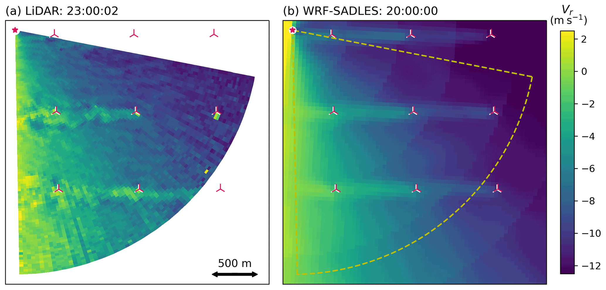
Figure 11 (a) Line-of-sight (LOS) velocity from a horizontal lidar scan at the FINO1 station around 23:00 UTC. (b) Simulated LOS velocity from WRF-SADLES at 20:00 UTC.

Figure 11a shows the LOS velocity from a horizontal lidar scan from the FINO1 station at 23:00 UTC, at which the wind blows from the east, and the full wake effect of a wind turbine from the Alpha Ventus is recorded. The lidar scan covers a circular sector extending from a height of 23.5 m with a small elevation angle of 1.55°, reaching a radius of 2500 m and encompassing five turbines. The signal reaches a height of approximately 90 m at the outer radius, corresponding to the hub height of the turbines. Turbine wakes are clearly visible, except for the middle turbine on the right, which is likely non-operational.

For comparison, in Fig. 11b, the simulated LOS velocity from the WRF-SADLES model at 20:00 UTC with an easterly wind direction is presented. Generally, there is good agreement between the model and lidar observations. Nevertheless, compared to the lidar data, the WRF-SADLES wind speed distribution is smoother. This is likely attributable to the coarse resolution capturing the small-scale turbulence explicitly.

4.3 A brief example of farm-to-farm interaction

In this section, we briefly demonstrate the use of WRF-SADLES to simulate an example of farm-to-farm interaction. The LESs were conducted for domains D04 and D05 from 06:00 to 12:00 UTC on 24 September 2016. The mesoscale domains commenced earlier at 00:00 UTC to initialize the environmental conditions. This time frame was selected due to the relatively steady wind direction from the south-southwest, allowing farm-to-farm interactions between Alpha Ventus and the wind farm to the southwest. To quantify the influence of this farm, we set up two experiments: the first experiment (EXP1) incorporated all four wind farms, while the second experiment (EXP2) excluded all wind farms except Alpha Ventus.

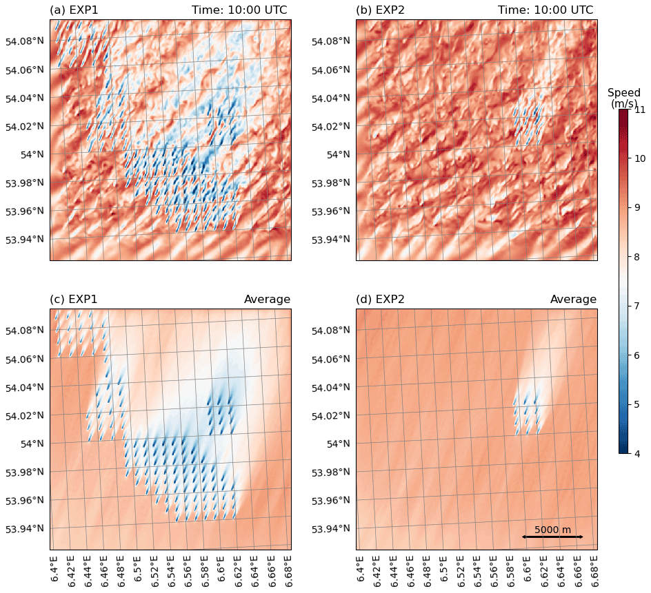
Figure 12 (a, b) A snapshot of wind speed in the 40 m domain (D05) at the height of 90 m at 10:00 UTC on 24 September 2016. (c, d) The 4 h average wind speed (from 08:00 UTC to 12:00Z on 24 September 2016).

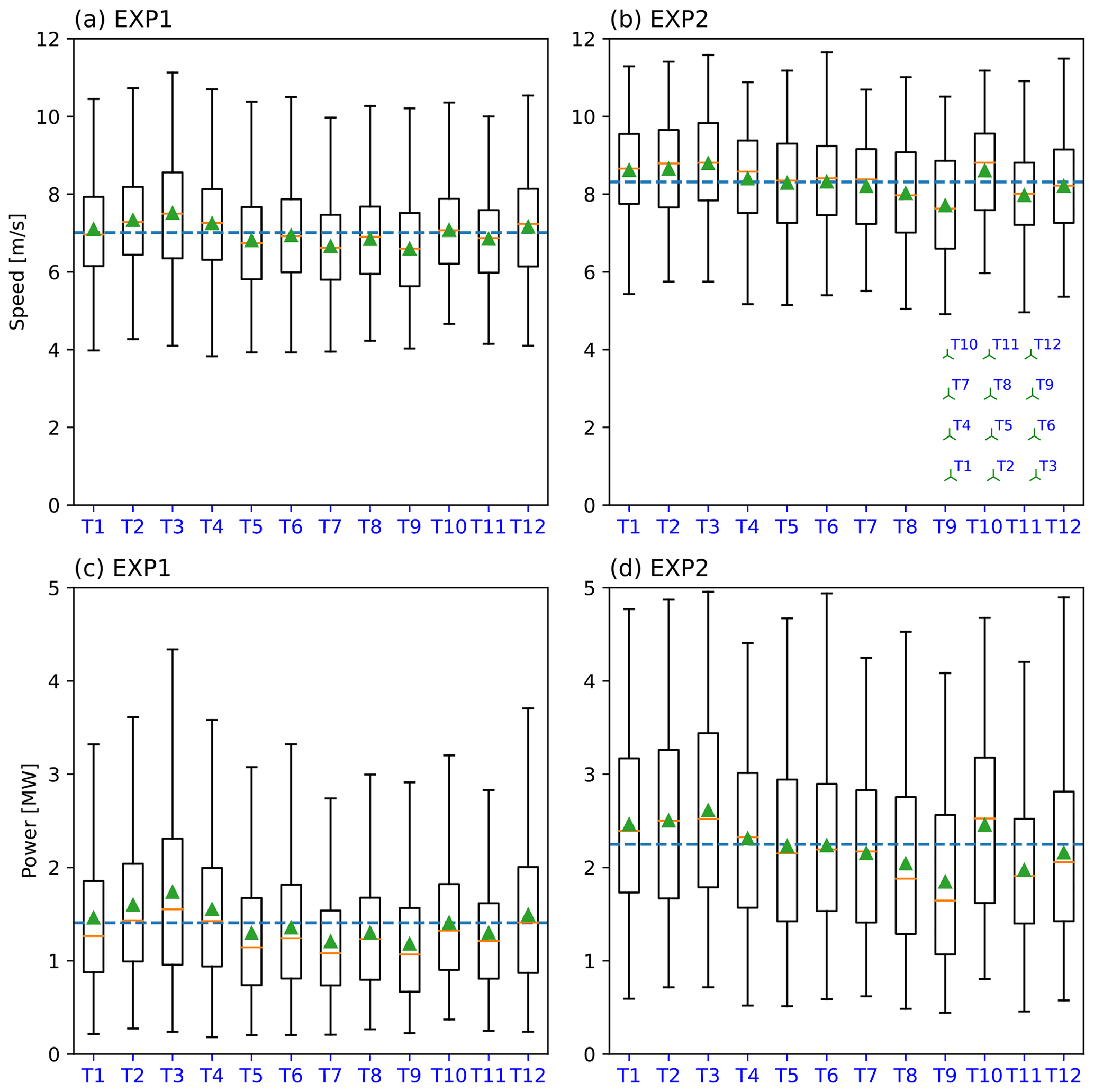
Figure 13 Boxplots of 4 h (from 08:00 to 12:00 UTC on 24 September 2016) for ambient wind speeds (a, b) and turbine powers (c, d) for the turbines in the Alpha Ventus wind farm. The average values (dashed blue lines) are 7 and 8.3 m s⁻¹ for (a) and (b) and 1.4 and 2.25 MW for (c) and (d), respectively. The layout of the turbines in the Alpha Ventus wind farm is shown on the bottom right of panel (b).

Figure 12a and b show an example snapshot of the wind speed at the Alpha Ventus hub height (90 m) for the 40 m LES domain for the two experiments at 10:00 UTC on 24 September 2016. Thanks to the cell perturbation at the southern boundary, the turbulence quickly becomes fully developed after a short distance from the southern border (or roughly 10 % of the domain width). This allows the turbulence flow to become quasi-steady when it reaches the turbines in the wind farms. Such turbulence development is important because it affects the wake recovery behind the turbines.

Figure 12c and d show the 4 h average wind speed from 08:00 to 12:00 UTC on 24 September 2016. During this time window, the wind direction is relatively steady from the south-southwest, enabling us to address the potential impact of turbine wakes in the Alpha Ventus wind farm. Before coming to the wind farm, the average speed is slightly above 8 m s⁻¹ and is distributed uniformly because of the small size of the domain. In EXP1, the south-southwesterly wind direction and the wake from a nearby wind farm significantly reduce the wind speed reaching Alpha Ventus (Fig. 12c). Conversely, with no upstream wind farm in EXP2, the averaged ambient wind speed remains nearly unchanged when approaching the Alpha Ventus wind farm. Consequently, the wake effect within Alpha Ventus is weaker in EXP1 compared to EXP2. This highlights the significant impact of farm-to-farm interaction, as evidenced by the larger difference in wind speed between the two scenarios compared to the variation within Alpha Ventus itself. In both experiments, the collective wave effects from the wind farm reduce the average wind speed to a distance over 10 km downstream.

Both experiments also show evidence of some intra-farm interaction where the wind speed deficits for turbines at the northeast corner are slightly smaller than those at the front south and west sides. However, due to the specific wind direction, the wakes generated by the turbines do not directly impact the turbines in the following rows. Consequently, the variation in wind speed deficit between turbines within the Alpha Ventus wind farm is minimal compared to the overall difference between the two experiments.

Figure 13 also shows the intra-farm interaction is small compared to farm-to-farm interaction. For each experiment, the variation in the ambient wind speed is smaller than the difference between EXP1 and EXP2. The average ambient wind speed at the Alpha Ventus wind farm is significantly lower when the wind farm to the south is present (EXP1) compared to when there are no wind farms (EXP2). For EXP1, the average ambient wind speed is 7 m s⁻¹, as shown in Fig. 13a. In contrast, when there are no nearby wind farms (EXP2), the average ambient wind speed is 8.3 m s⁻¹, as shown in Fig. 13b. This represents a reduction in wind speed of about 16 %. However, due to the non-linear nature of the turbine power curve, the power reduction resulting from the farm-to-farm interaction (Fig. 13) is larger. The average power for EXP2 is approximately 2.25 MW, while the average power for EXP1 is 1.4 MW, corresponding to a reduction of about 38 %.

5 Conclusion

In this paper, we presented our implementation of a Simple Actuator Disk model for Large-Eddy Simulation (SADLES) within the Weather Research and Forecasting model (WRF-SADLES). Unlike other previous implementations of wind turbine parameterization within WRF, such as the general actuator disk (GAD) (Mirocha et al., 2014; Kale et al., 2022), WRF-SADLES only requires the power curve and thrust coefficient curve – the same information used in the wind farm parameterization (WFP; Fitch et al., 2012) that is already included in WRF. The purpose of WRF-SADLES is to explicitly simulate the wakes of multiple wind farms in nested downscaling applications from realistic atmospheric conditions. Therefore, the target resolution of WRF-SADLES is of the order of 10 m, which is lower than the resolutions of a few meters in typical applications using WRF-GAD (e.g., Mirocha et al., 2014; Kale et al., 2022), to reduce the computational demand.

WRF-SADLES employs the traditional actuator disk model, representing the turbine as a thin disk that generates thrust, slowing down ambient wind speed. In our idealized experiments with a single 5 MW turbine (Sect. 3), WRF-SADLES demonstrated good agreement compared to a dedicated LES model (the PALM model), whose actuator disk model uses blade element theory, providing a more comprehensive representation. Interestingly, at our target resolution of 30 m, WRF-SADLES exhibited better agreement with the 10 m resolution than the PALM model.

We assessed two methods for evaluating the axial induction factor: direct evaluation (Option 1) using data points at and in front of the turbine and inferred evaluation (Option 2) using one-dimensional momentum theory. The results demonstrated strong agreement between the two methods. We recommend employing Option 2 to avoid potential issues associated with Option 1, as discussed in Sect. 2.1.

Additionally, we experimented with adding subgrid-scale turbulence kinetic energy (TKE) at the actuator disk, similar to the approach by Fitch et al. (2012). However, the effect of added TKE only influenced a short distance from the turbine, and the far-wake structures, including wake deficit and turbulent intensity, remained similar regardless of the presence of added TKE. Therefore, we recommend deactivating this option (i.e., f_TKE=0) for practical application, partly because the rationale behind the method does not reflect reality.

We conducted a brief validation of WRF-SADLES using observational data from the FINO1 offshore meteorological mast station. These data included measurements from a cup anemometer at 90 m height, as well as vertical and horizontal wind profiles obtained by lidar. The simulation downscales the ERA5 global reanalysis from a coarse resolution (approximately 31 km) to a turbine-scale resolution (40 m). This downscaling is achieved through a system of five nested domains, with the outer three domains simulating mesoscale processes and the two inner domains simulating eddy turbulence. The results demonstrate good agreement in the wake deficit observed at the FINO1 location between WRF-SADLES and the actual observations. However, there is a discrepancy in the timing of the wake deficit occurrence. We attribute this error not to the turbine model itself but to the intermediate 200 m resolution LES domain. This domain serves as the transitional zone between the mesoscale and microscale, where turbulence activity is not accurately represented.

Finally, we present an example of farm-to-farm interaction at the Alpha Ventus wind farm near the FINO1 station. Here, the wind farm to the southeast of Alpha Ventus leads to a reduction in ambient wind speed by approximately 16 %, resulting in an average turbine power decrease of 38 % during a 4 h analysis window.

We have made our code openly available to promote further research in wind energy. Our code distribution includes our implementation of the cell perturbation method (Muñoz-Esparza et al., 2014), crucial for turbulence development in nested LES. While WRF-SADLES demonstrates promising capabilities for meso-to-micro downscaling, addressing issues in the transition resolutions will be crucial for enhancing wake predictions. Future development areas for WRF-SADLES could involve implementing yaw misalignment to enable wake deflection and investigating turbine yaw control strategies.

Appendix A: Additional WRF namelist options

Table A1 Summary of WRF-SADLES namelist options.

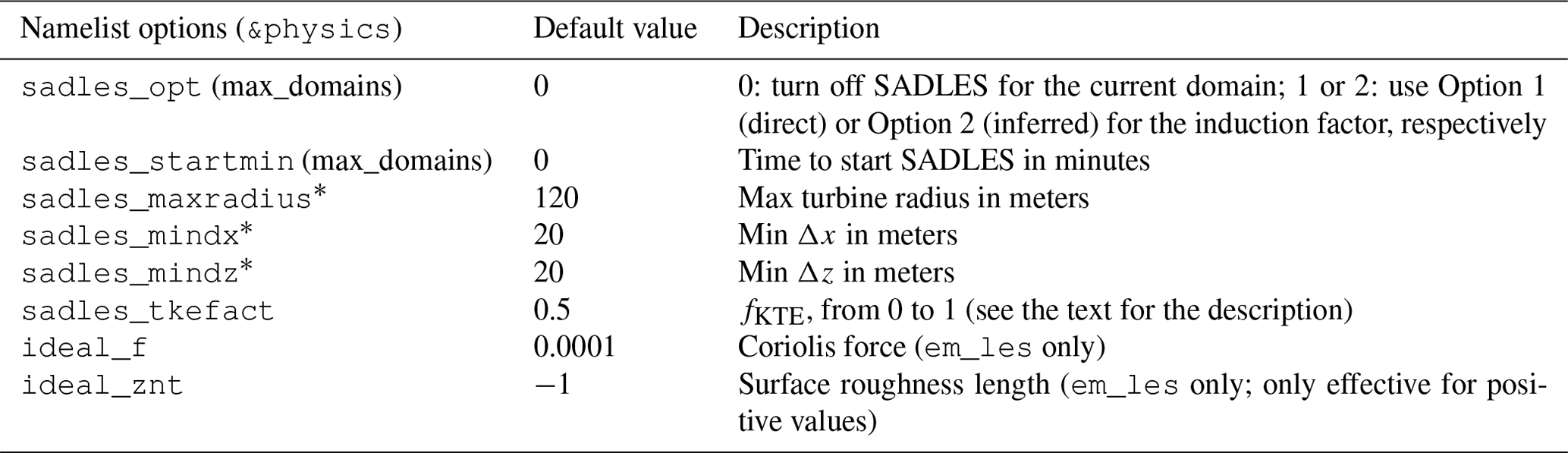
^* These values are used to allocate arrays within the SADLES module.

Table A2 Summary of cell perturbation namelist options.

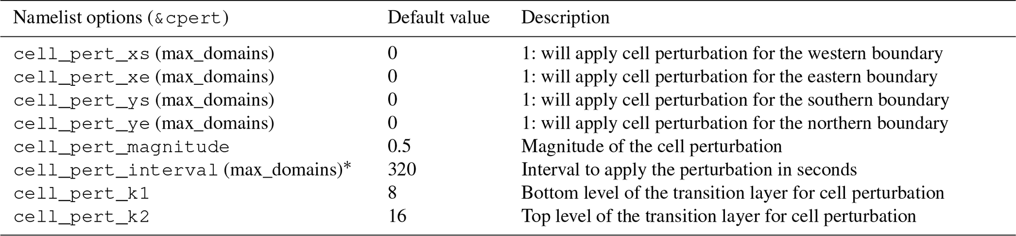
^* The interval should be approximately $\frac{\mathrm{8}\mathrm{\Delta }x}{U}$, where U is the average wind speed during the simulation. For example, with Δx=200 m and U=5 m s⁻¹, the interval will be approximately $\frac{\mathrm{8}\left(\mathrm{200}\text{ m}\right)}{\mathrm{5}{\text{ m\hspace{0.17em}s}}^{-\mathrm{1}}}=\mathrm{320}$ s.