the Creative Commons Attribution 4.0 License.
the Creative Commons Attribution 4.0 License.
 | 24 May 2024
Investigating ground-level ozone pollution in semi-arid and arid regions of Arizona using WRF-Chem v4.4 modeling
Yafang Guo
Chayan Roychoudhury
Mohammad Amin Mirrezaei
Rajesh Kumar
Armin Sorooshian
Avelino F. Arellano
Ground-level ozone (O3) pollution is a persistent environmental concern, even in regions that have made efforts to reduce emissions. This study focuses on the state of Arizona, which has experienced elevated O3 concentrations over past decades and contains two non-attainment areas as designated by the U.S. Environmental Protection Agency. Using the Weather Research and Forecasting with Chemistry (WRF-Chem) model, we examine O3 levels in the semi-arid and arid regions of Arizona. Our analysis focuses on the month of June between 2017 and 2021, a period characterized by high O3 levels before the onset of the North American Monsoon (NAM). Our evaluation of the WRF-Chem model against surface Air Quality System (AQS) observations reveals that the model adeptly captures the diurnal variation of hourly O3 levels and the episodes of O3 exceedance through the maximum daily 8 h average (MDA8) O3 concentrations. However, the model tends to overestimate surface NO2 concentrations, particularly during nighttime hours. Among the three cities studied, Phoenix (PHX) and Tucson (TUS) exhibit a negative bias in both hourly and MDA8 O3 levels, while Yuma demonstrates a relatively large positive bias. The simulated mean hourly and MDA8 O3 concentrations in Phoenix are 44.6 and 64.7 parts per billion (ppb), respectively, compared to observed values of 47.5 and 65.7 ppb, resulting in mean negative biases of −2.9 and −1.0 ppb, respectively.
Furthermore, the analysis of the simulated ratio of formaldehyde (HCHO) to NO2 (; FNR), reveals interesting insights of the sensitivity of O3 to its precursors. In Phoenix, the FNR varies from a VOC (volatile organic compound)-limited regime in the most populated areas to a transition between VOC-limited and NOx-limited regimes throughout the metro area, with an average FNR of 1.15. In conclusion, this study sheds light on the persistent challenge of ground-level O3 pollution in semi-arid and arid regions, using the state of Arizona as a case study.
- Article
(17961 KB) - Full-text XML
-
Supplement
(6024 KB) - BibTeX
- EndNote


Ground-level ozone (O3), or tropospheric O3, is a harmful air pollutant that affects human health and plants (Anderson, 2009; Reich, 1987; Iriti and Faoro, 2009; Wang et al., 2017; Lippmann, 1989; Manisalidis et al., 2020). O3 concentrations are affected by meteorological conditions and the concentrations of precursors (Vingarzan, 2004; Wang et al., 2017; Fiore et al., 2002; Jacob, 2000; Monks et al., 2015). Meteorological factors include intensity of solar radiation, temperature (T), relative humidity (RH), winds, pressure, and boundary layer height (Trainer et al., 2000). The precursors of O3 include nitrogen oxides (NOx) and volatile organic compounds (VOCs). Besides its significant role in forming O3, NOx, particularly NO2, is also an important pollutant mainly emitted by human activities.
With projections indicating the expansion of aridity zones due to climate change in the future (Asadi Zarch et al., 2017; Achakulwisut et al., 2019; Straffelini and Tarolli, 2023; Huang et al., 2017), there is an anticipated rise in O3 levels under more drought and elevated temperature conditions (Achakulwisut et al., 2019), thereby posing potential challenges to overall air quality, vegetation, and public health. In the face of these projections, there is an undeniable sense of urgency in advancing our comprehension of O3 production mechanisms and refining forecasting model skills, especially within urban arid regions. This imperative arises from the acknowledgement that urban areas in arid climates face a distinctive set of challenges marked by exceptionally low precipitation, elevated temperatures, and unique vegetation. Gaining such insights is crucial for generating effective strategies to mitigate the negative impacts on air quality, vegetation, and the health of urban populations in response to shifting climatic conditions.
Because of the Clean Air Act, average NO2 concentrations have decreased substantially in the US since the 1990s (U.S. Environmental Protection Agency, 2012). For example, the annual 98th percentile of daily maximum 1 h average NO2 was reduced from 42 to 33 ppb with a 21 % decrease in the national average from 2010 to 2022 (EPA, 2023a). VOCs in the atmosphere are generally emitted from two major sources: human activity and biogenic volatile organic compounds (BVOCs) produced by plants. In the US, VOC emission data are tracked by the NEI. According to NEI data, in Maricopa County, where the city of Phoenix resides, total estimated VOC emissions from anthropogenic sources, excluding forest wildfires and prescribed burns, decreased by 35 % between 2008 and 2020 (from 0.19 to 0.13 million tonnes). Most anthropogenic emissions reductions were observed among on-road mobile sources and other industrial processes. As a result, O3 levels have substantially decreased across much of the US (Cooper et al., 2012; Parrish et al., 2022). In 2015, the U.S. EPA lowered the O3 National Ambient Air Quality Standard (NAAQS) to 70 parts per billion (ppb). The design value is defined as the annual fourth-highest maximum daily 8 h average (MDA8) O3 concentration, averaged over 3 years. Any area that does not meet this standard is designated as a non-attainment area (NAA). Despite the nationwide decrease of O3 precursors and O3 concentrations, there are still areas where O3 levels exceeded the 2015 NAAQS standard of 70 ppb in 2017 (U.S. Environmental Protection Agency, 2015). Therefore, for these areas, it is critical to have a detailed understanding of the chemical and meteorological processes influencing O3 formation so that better pollution control can be put in place to reduce O3 levels.
Identifying and quantifying the various sources that contribute to the formation of O3 is challenging due to the complicated nature of atmospheric chemistry and variability of O3 precursors (Duan et al., 2008; Fang et al., 2021; He et al., 2019; Odman et al., 2009; Yang et al., 2021; Zare et al., 2014; Zhan et al., 2023; Trainer et al., 2000). First, O3 formation is a complex process that involves the interaction of multiple precursor pollutants, such as NOx and VOCs, under the influence of sunlight. The chemistry behind these reactions can be highly nonlinear and dependent on numerous variables (e.g., temperature, moisture, cloud cover, and solar radiation) (Trainer et al., 2000). This nonlinearity makes it challenging to predict how changes in emissions will impact O3 concentrations. In addition, O3 is not limited to areas where its precursors are emitted as it can be transported over long distances. This makes it difficult to attribute O3 levels solely to local sources, as regional and even global factors can influence local concentrations (Vingarzan, 2004; Monks et al., 2015).
In Arizona, the Phoenix-Mesa metropolitan area is currently designated as a moderate NAA for O3 and has ranked among the top five of most polluted cities for O3 in the last 5 years (source: https://www.lung.org/research/sota/city-rankings/most-polluted-cities, last access: 20 September 2022). Another NAA is Yuma County. Unlike Maricopa County, Yuma is a rural region that has a much lower population and emissions. With Yuma being located on the border of Mexico to the south and southwest and California to the west, its O3 levels thus are significantly impacted by both international and inter-state transport. Qu et al. (2021) investigated the sources of O3 pollution in Yuma, Arizona, and found strong international influences from northern Mexico on 12 out of 16 O3 exceedance days. They also performed a sensitivity study with the GEOS-Chem model and found that reducing emissions in Arizona alone would have a minimal impact on mitigating O3 exceedances in Yuma, with only a 0.7 % reduction in MDA8 O3. In contrast, reducing emissions in Mexico is estimated to contribute to an 11 % reduction in O3 during these exceedances, bringing MDA8 O3 in Yuma below the standard. Li et al. (2015) applied Weather Research and Forecasting with Chemistry (WRF-Chem) with sensitivity experiments and showed that Arizona emissions have a dominant impact on MDA8 O3 concentrations in Phoenix, while southern California's contributions range from a few ppb to over 30 ppb.
While long-range transport of precursors and O3 into Arizona does occur, the primary contributor to O3 levels remains the in situ production resulting from local emissions. Because most of Arizona is a semi-arid and arid region with a unique southwest natural environment including weather, climate, and desert plants, it is important to understand how the extreme heat, low moisture, and year-round desert shrubs contribute to O3 production in order to minimize O3 exceedances and improve air quality forecasting (Sorooshian et al., 2024). Additionally, even though Arizona is a typical desert weather region with high temperatures and low moisture year-round, during the North American Monsoon (NAM) the primary wind flow in Arizona shifts from westerly and southwesterly to southerly and southeasterly, resulting in elevated moisture from the Pacific Ocean and the Gulf of California. Furthermore, unlike the other O3-polluted regions in the eastern US, which are mainly forest ecosystems, most of Arizona experiences little precipitation – less than 25 cm or 25 to 50 cm of rain per year (Paul et al., 2002). The BVOCs are also quite unique in the arid climate region. Geron et al. (2006) found out that in the Mojave Desert and Sonoran Desert regions of the western US where Arizona is, of all the 13 common desert plant species, only two of the species emitted isoprene (the most abundant BVOC) indicating that this type of ecosystem is not likely a strong source of isoprene compared to forest ecosystems.
In Sect. 2 we first discuss the climatology of Phoenix, as a representation of southwestern Arizona, and then describe the datasets employed and the setup of the WRF-Chem model. In Sect. 3 we present analyses of model evaluation with observations including meteorological fields, O3, and precursors. The analyses of O3 exceedance and VOC-NOx sensitivity are also included. Section 4 summarizes the main conclusions of this study.
This research focuses on the study of O3 in the state of Arizona in the US. In this section, we begin with introducing the available datasets applied to evaluate the WRF-Chem model including observational datasets from EPA AQS and PAMS network, reanalysis using CMAQ modeling, radiosonde measurements, and regional forecasts. A description of the study region is then given, and this is followed by the model description and configurations.
2.1 EPA AQS surface observations
We use the hourly and daily surface in situ observations of O3, CO, NO2, and meteorological fields such as T, RH, and winds from the EPA AQS monitoring network (Demerjian, 2000). Sites within each city were selected based on their availability during the study periods for each parameter. For instance, for O3 measurements, 10 sites were selected in Phoenix, 7 in Tucson, and 2 in Yuma. The information for each is listed in Table S2 in the Supplement. For evaluation purposes, we applied quality control to the raw data to exclude any values that were zero or negative before doing further analysis. To calculate the MDA8 O3, any days with more than eight continuous hourly data points missing were excluded from the analysis. Zero and negative values were treated as missing, while values below the method detection limit (MDL) were replaced with 0.5× MDL (Zhang et al., 2012).
2.2 EPA PAMS VOC measurements
The network of Photochemical Assessment Monitoring Stations (PAMS) established by the U.S. EPA plays a crucial role in monitoring and understanding ground-level O3 pollution in affected areas providing measurements of various O3 precursors, including VOCs. The list of measurements includes 63 different compounds with some of the most common VOC species like formaldehyde (HCHO), acetaldehyde, acetone, ethanol, and two monoterpenes (α-pinene and β-pinene; C10H16). The primary objective of these PAMS sites is to create a comprehensive database of O3 precursors and meteorological conditions to better understand local O3 formation, support the development of O3 models, and allow for the tracking of important trends in O3 precursor concentrations over time. The two PAMS monitor sites in Arizona are located in Phoenix (JLG Supersite: 04-013-9997) and Tucson (22nd & Craycroft: 04-019-1011). The sampling frequency for most VOCs is hourly averaged. For formaldehyde, the JLG Supersite uses the EPA's 3 d schedule with three 8 h averaged carbonyl samples per day on every third day.
2.3 Radiosonde data
High vertical resolution temperature profiles from radiosondes are applied to determine the planetary layer boundary height (PBLH) for WRF-Chem evaluations. Data from radiosondes launched at three different locations (Phoenix, Tucson, and Yuma) were downloaded. The radiosonde launches in Phoenix are active during the monsoon season, starting in mid-June and ending in late September while Tucson and Yuma conduct regular daily balloon launches. The launch times for Phoenix and Tucson are set at 00:00 and 12:00 UT, while Yuma operates two launch sites with schedules at 12:00, 18:00, and 21:00 UT. To estimate the PBLH, we use the bulk Richardson number method. The Richardson number is a dimensionless number used to assess atmospheric stability. The top of planetary layer boundary is marked by when the Richardson number exceeds a threshold of 0.25.
2.4 CMAQ reanalysis
A high-resolution (12×12 km2) air quality reanalysis over the contiguous US (CONUS) is available from 2005–2018 (https://www.gcseglobal.org/development-air-quality-products, last access: 15 June 2023). This reanalysis is generated using a newly developed chemical data assimilation system that simultaneously assimilates aerosol optical depth (AOD) retrievals from the Moderate Resolution Imaging Spectroradiometer (MODIS) and carbon monoxide (CO) retrievals from the Measurement of Pollution in the Troposphere (MOPITT) in the Community Multiscale Air Quality (CMAQ) model. The WRF model provides meteorological input for CMAQ simulations over the CONUS. This dataset offers a suite of air quality products, e.g., PM2.5, PM10, O3, and NO2. In this study, beyond the ground-based EPA observations we expand our analysis by incorporating this reanalysis dataset to enhance the evaluation of O3 levels across Arizona.
2.5 ADEQ forecasts
The Arizona Department of Environmental Quality (ADEQ) produces 5 d hourly air quality forecasts for locations across Arizona (https://www.azdeq.gov/forecast, last access: 4 April 2023). Specifically for our study region, forecasts are released Monday through Friday and include O3, PM10, and PM2.5. The forecast values are for the monitor with the highest MDA8 O3 concentration for a given day within the Phoenix-Mesa NAA and the Tucson area, whereas for Yuma it is a single monitor (Yuma Supersite).
2.6 Description of study region and time period
The climate of the southern and southwestern parts of Arizona (Sonoran Desert) is dry and hot, with much of the region characterized as arid. Our primary interest is in three major cities: Phoenix, Tucson, and Yuma. Phoenix, the most populated city, is designated as an O3 NAA by EPA along with the entire metro area; Tucson, which is the second largest city in the state, experiences mild O3 pollution but gets stronger influence from the monsoon and Mexico; Yuma, situated near both California and Mexico, is a representation of an arid section of the Sonoran Desert and also designated as a NAA with clean data determination by EPA.
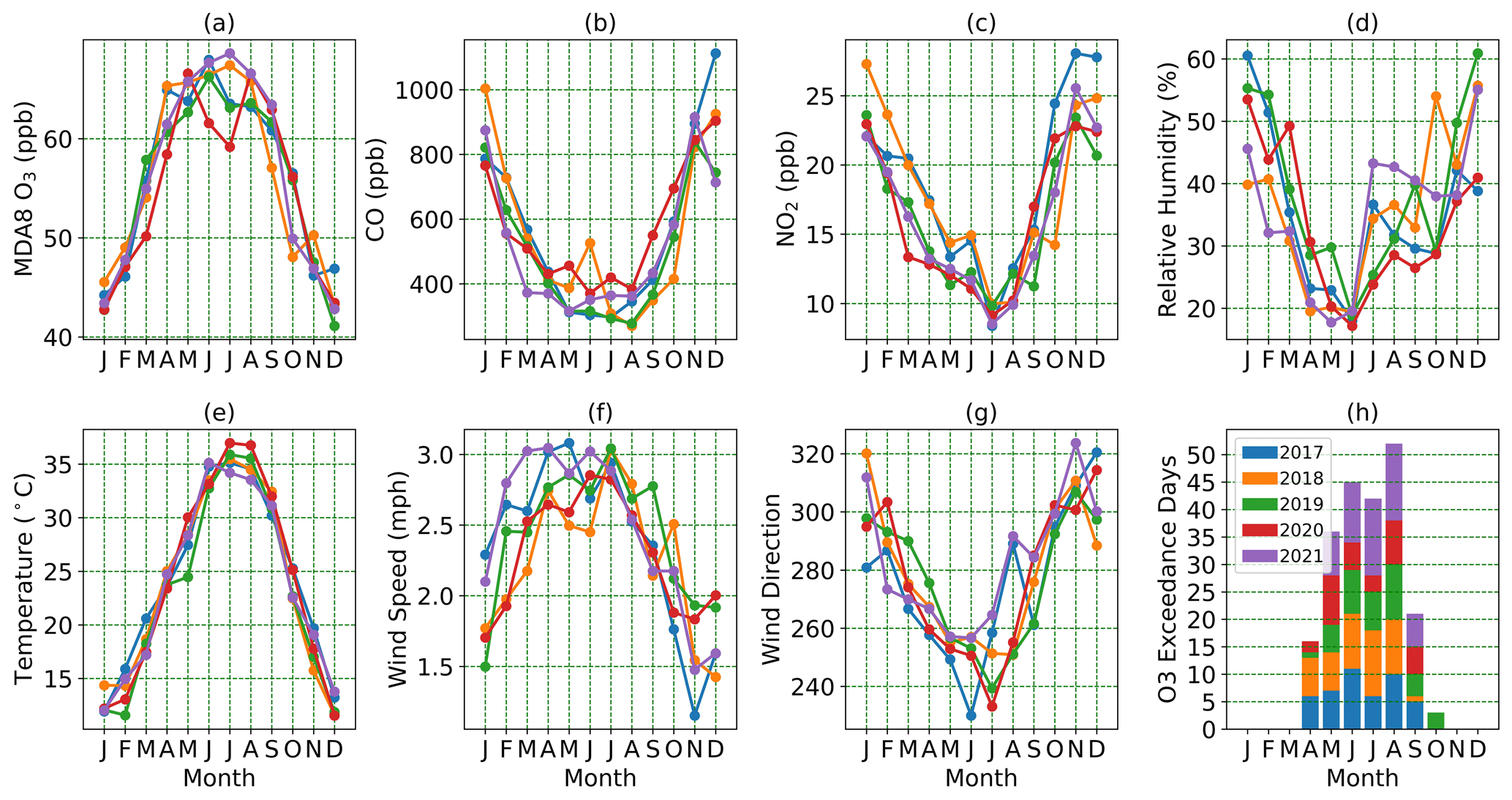
Figure 1Monthly mean of Phoenix surface (a) MDA8 O3, (b) CO, (c) NO2, (d) relative humidity (RH), (e) temperature (T), (f) wind speed, (g) wind direction, and (h) number of exceedance days for years between 2017 and 2021, derived from EPA criteria gases and meteorological daily summary data of a single site (Phoenix JLG Supersite).
Shown in Fig. 1 are the monthly mean surface air values of MDA8 O3, CO, and NO2 and meteorological fields of RH, T, wind speed, and wind direction in the city of Phoenix. These monthly values were derived from averaging the daily EPA AQS data collected over a 5-year period from 2017 to 2022 at the Phoenix JLG Supersite. The MDA8 (Fig. 1a) exhibits peaks during the summer months, spanning from April to September, except for the year 2020 when the COVID-19 pandemic began. On the other hand, the monthly CO, NO2, and RH show an opposite trend, with their lowest values observed during the summer months. RH is the lowest in June and then increases as the monsoon arrives in July, followed by decreases in September after the monsoon ends. Besides the COVID-19 factor, 2020 is ranked as the second driest year in Arizona's history, with a statewide precipitation level of only 6.63 in. (168.4 mm; NWS Phoenix, 2020). Figure 1d shows that the RH levels during late 2020 (red line) and early 2021 (purple line) were the lowest across the 5-year period. Additionally, the temperature during the summer of 2020 (Fig. 1e) was also the highest. For winds, the windiest seasons are spring and summer, and the wind direction varies throughout the year. The wind direction is determined by taking the inverse tangent of the total zonal and meridional wind components, which are derived from the daily maximum wind speed and its corresponding direction. Summer months exhibit mostly westerly winds, while winter months consist of more easterly winds (Fig. 1f–g). Shown in Fig. 1h is the distribution of monthly O3 exceedance days at the JLG Supersite in Phoenix (site no. 04-013-9997). An O3 exceedance day occurs when the MDA8 O3 is greater than 70 ppb on that day. The exceedance days are mostly recorded from April to September, referred to here as the “ozone season”. In the months of June and July in the year 2020, the MDA8 O3 (Fig. 1a) and exceedance days (Fig. 1h) were substantially lower than in other years, and the reason could be related to the COVID-19 pandemic. The pandemic's stay-at-home period resulted in much lower traffic levels and hence reduced anthropogenic emissions.
Based on these monthly results, we choose the month of June (dry summer), when O3 levels, temperature, and winds are high and the moisture level is still low. It is also intended to mitigate the impact of the heavy precipitation that typically accompanies the monsoon. Additionally, since we focus on the desert area, dust storm events can significantly impact the O3 photolysis, hence the concentrations. According to Lader (2016), the highest frequency of dust storm events happens during the active Monsoon season (in July and August). Therefore, we have chosen June as our main study period to reduce the impacts of dust. We apply the WRF-Chem model (v4.4) with state-of-art configurations to simulate the O3 concentrations over Arizona. Numerical simulations were conducted during June between 2017 and 2021 for a total of 5 years. Furthermore, the ozone season in 2017 was also simulated as our base year. The following sections describe the datasets analyzed herein and the configuration used for the WRF-Chem simulations.
2.7 WRF-Chem setup
The Weather Research Forecasting coupled with Chemistry (WRF-Chem) (Grell et al., 2005) model is a fully coupled meteorology–chemistry transport model developed by the National Center for Atmospheric Research (NCAR). This study uses WRF-Chem v4.4 to simulate O3 in Arizona. With our ultimate goal of establishing an operational forecasting and analysis system for Arizona in the future, we have configured the model using the NCAR WRF-Chem forecasting system as a reference (https://www.acom.ucar.edu/firex-aq/forecast.shtml, last access: 15 August 2023). The comprehensive parameterization schemes are provided in the following list. The Model for Ozone and Related Chemical Tracers (MOZART-4, Emmons et al., 2010) is selected for the gas-phase chemistry, coupled with the Goddard Chemistry Aerosol Radiation and Transport (GOCART, Chin et al., 2002) for aerosol chemistry with wet scavenging enabled. The standard MOZART-4 mechanism includes 85 gas-phase species, 12 bulk aerosol compounds, in addition to 39 photolysis and 157 gas-phase reactions. It also includes an updated isoprene oxidation scheme and a better treatment of volatile organic compounds, with three lumped species to represent alkanes and alkenes with four or more carbon atoms and aromatic compounds (called BIGALK, BIGENE, and TOLUENE) (Emmons et al., 2010). The new updated Tropospheric Ultraviolet and Visible (TUV) photolysis option, based on standalone TUV version 5.3, is employed to calculate the photolysis rates. This new TUV option uses O3 climatology distributed from the model top (∼20 km) to 50 km. Initial and lateral boundary conditions are supplied every 6 h from both the Global Forecast System (GFS) with a horizontal grid spacing of 1° for meteorology and the Community Atmosphere Model with Chemistry (CAM-Chem) (Lamarque et al., 2012; Tilmes et al., 2015) for chemistry. Biogenic emissions are calculated online with the Model of Emissions of Gases and Aerosols from Nature (MEGAN, v2.1) using the simulated meteorological conditions while running WRF-Chem (Guenther, 2007; Guenther et al., 2006). Note that MEGAN v2.1 currently is only compatible with the CLM4 (Community Land Model Version 4, Oleson et al., 2010) land surface model. The anthropogenic emissions used in this study are obtained from 2017 National Emissions Inventories (NEI2017) data provided by the U.S. EPA (https://www.epa.gov/air-emissions-inventories/2017-national-emissions-inventory-nei-data, last access: 20 June 2022) with a 4 km grid resolution covering the US and surrounding land areas. NEI emissions are then interpolated and regridded to model domain grids. Biomass burning emissions are calculated using the Fire Inventory from NCAR (FINNv2.5) (Wiedinmyer et al., 2023) and the online plume-rise model (Freitas et al., 2007). FINNv2.5 is based on fire counts derived from both satellite MODIS and VIIRS (Visible Infrared Imaging Radiometer Suite) active fire detection (Wiedinmyer et al., 2023). We employed the GOCART dust option in accordance with the GOCART aerosol scheme. The following key physics settings are also employed: Morrison double-moment microphysics (Morrison et al., 2009), RRTMG for long and short-wave radiation (Iacono et al., 2008), Eta Similarity for surface layer physics (Monin and Obukhov, 1954), the Unified Noah Land Surface Model (Tewari et al., 2004), the Yonsei University (YSU) planetary boundary layer (PBL) scheme (Hong, 2010), and the Grell–Freitas cumulus parameterization scheme (Grell and Freitas, 2014).
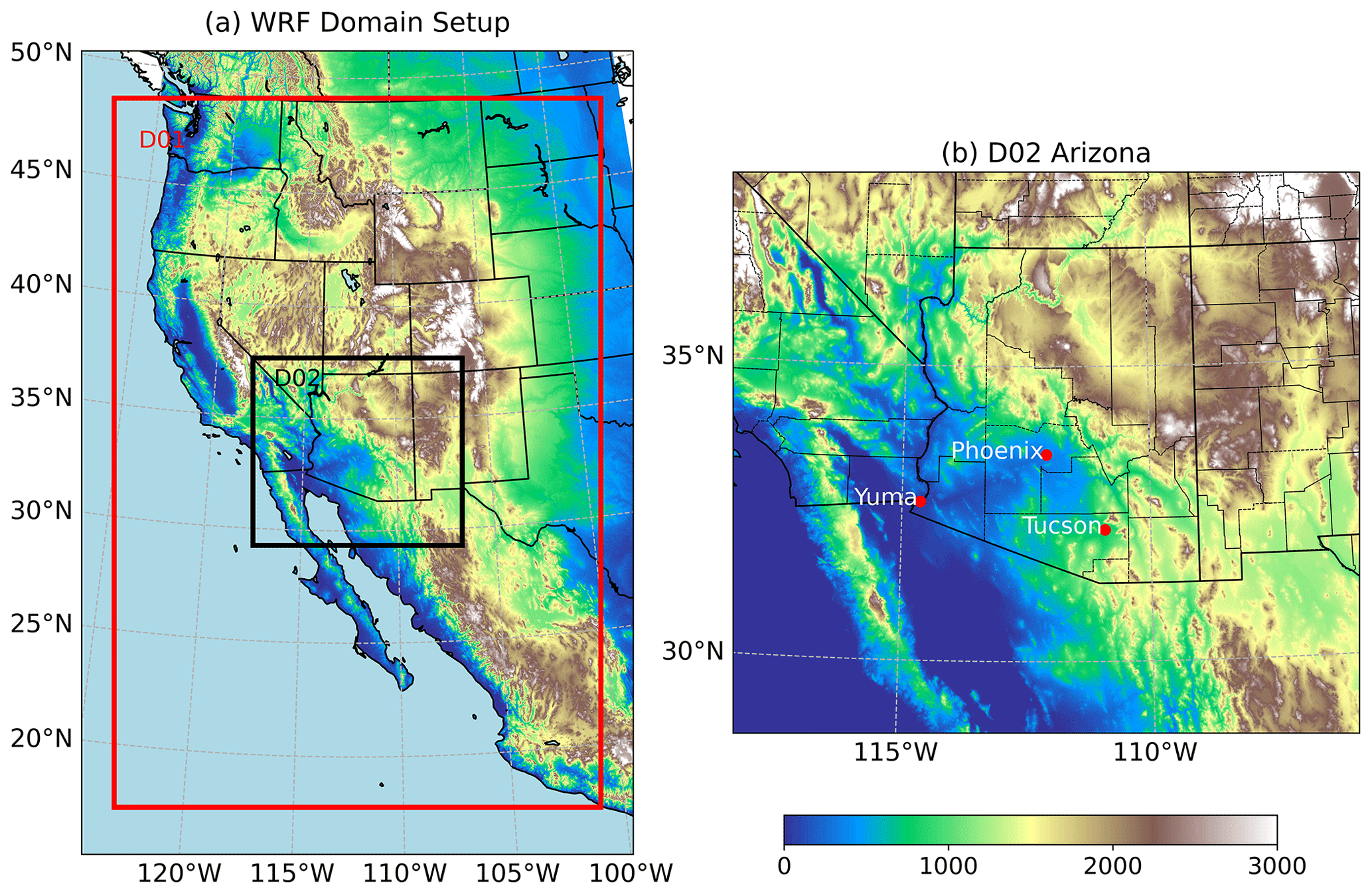
Figure 2(a) WRF-Chem domain setup for outer domain D01 and inner domain D02. (b) Geographic location of three Arizona cities: Phoenix, Tucson, and Yuma. Dashed black lines in (b) represent the county borders. Contours denote the elevation in meters over the continent.
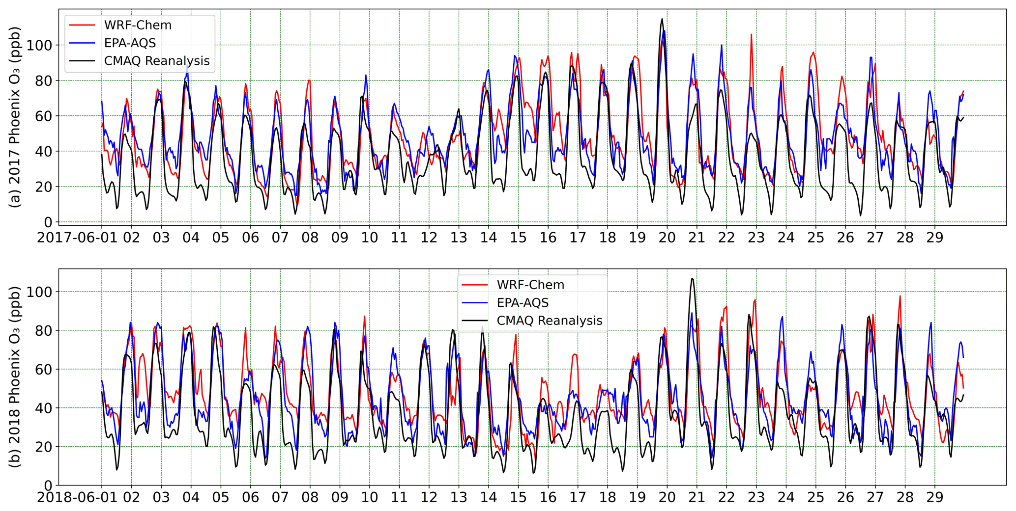
Figure 3WRF-Chem-simulated (red), EPA AQS (blue), and CMAQ reanalysis (black) hourly surface O3 concentrations in June 2017 (a) and 2018 (b) in Phoenix. Results are in universal time.
The model is configured with two nested grid domains consisting of 9 and 3 km horizontal grid spacing along with 34 vertical levels. Shown in Fig. 3 is the WRF-Chem domain setup. The parent domain (D01) covers the entire western U.S. with expansion to northern Mexico to better understand the wind shift from Mexico during NAM, while the nested domain (D02, Fig. 2b) focuses on Arizona. Both domains are centered in the Phoenix metropolitan area. D01 features 271 and 394 horizontal grids, while D02 is characterized by 349 and 313 horizontal grids. The topography in Fig. 2b (color contours) shows that Phoenix is located in about the center of a valley, called Salt River Valley. The WRF-Chem run periods are specifically designed to be the month of June between 2017 and 2021, with each run consisting of a total of 33 simulation days, including a 3 d spin-up in late May and 30 d in June.
3.1 Model evaluations
We begin by evaluating the simulated diurnal and monthly variations of meteorological fields and major air pollutants using the AQS monitor site and PAMS observations. Shown in Fig. 3 is the time series of Phoenix hourly surface O3 concentrations in June for the years 2017 and 2018. CMAQ air quality reanalysis datasets are also included for evaluation. The AQS observations for a particular city are calculated as the average of hourly or maximum daily 8 h average (MDA8) O3 levels obtained from all selected sites. These observations are subsequently compared with the mean simulated O3 concentration within the corresponding area. The diurnal pattern of O3 concentrations is clearly discernible, with peak levels occurring during the afternoon and reaching their lowest points at night. In general, the WRF-Chem model effectively captures these daily O3 concentration patterns. Conversely, the reanalysis dataset notably underestimates O3 levels during the nighttime. Notably, in June 2017, an extreme O3 event occurred, characterized by O3 levels exceeding 80 ppb and lasting for 9 d, starting on 14 June 2017. On 20 June, O3 levels even reached 100 ppb. The model effectively simulates this exceptional event, while the reanalysis dataset tends to overestimate this peak.
Table 1Mean statistics of WRF-Chem hourly O3 and evaluation with respect to EPA AQS observations in June for years 2017 to 2021. R is the Pearson correlation coefficient, MB is the mean bias, ME is the mean error, RMSE is the root-mean-square error, NMB is the normalized mean bias, NME is the normalized mean error, MNB is the mean normalized bias, MNE is the mean normalized error, MFB is the fractional bias, and MFE is the fractional error.
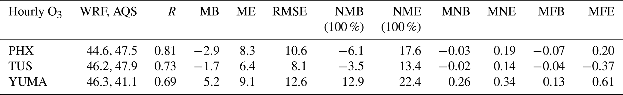
Listed in Table 1 are the statistical metrics comparing hourly concentrations from the WRF-Chem to the AQS monitoring sites at three different locations: Phoenix (PHX), Tucson (TUS), and Yuma (YUMA). The statistics include Pearson correlation coefficient (R), mean bias (MB), mean error (ME), root-mean-square error (RMSE), normalized mean bias (NMB), normalized mean error (NME), mean normalized bias (MNB), mean normalized error (MNE), fractional bias (MFB), and fractional error (MFE). For hourly O3, the correlation (R) indicates that all locations show a positive correlation, with PHX having the highest at 0.81, followed by TUS at 0.73, and YUMA at 0.69. The negative MB suggests that in PHX (−2.9 ppb) and TUS (−1.7 ppb) WRF-Chem underestimates the O3 concentration, while YUMA (5.2 ppb) suggests an overestimate. PHX and TUS generally exhibit smaller biases and errors compared to YUMA. Additionally, YUMA has the highest variability in errors and the highest NME and RMSE values, indicating less agreement with AQS data compared to PHX and TUS.
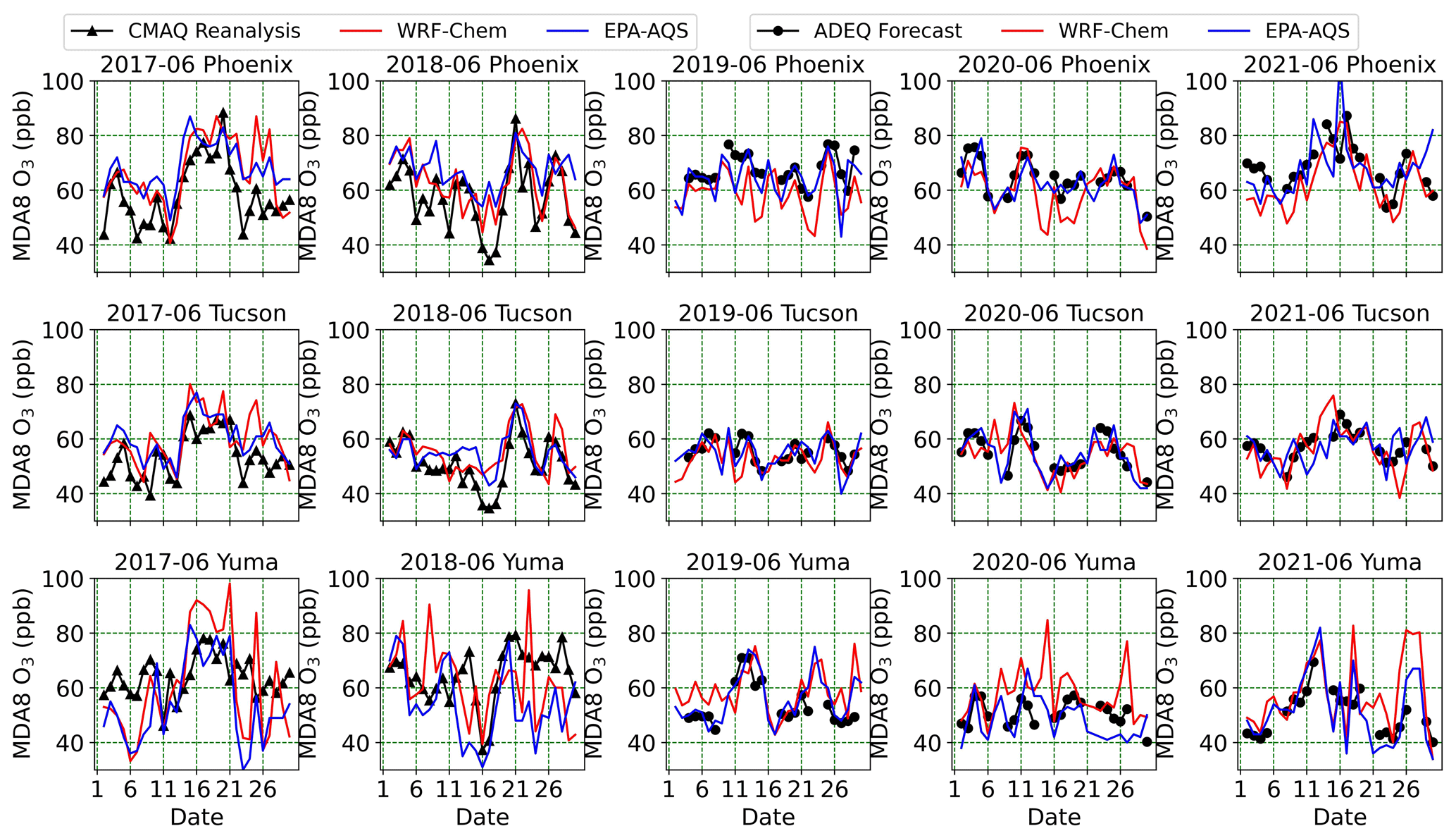
Figure 4WRF-Chem simulated (red), EPA AQS (blue), CMAQ reanalysis (black triangle), ADEQ forecasts (black circles), and MDA8 O3 concentrations in June 2017–2021 for three major Arizonan cities: Phoenix, Tucson, and Yuma.
In addition to the hourly O3 evaluation, we have also examined the MDA8 (maximum daily 8 h average) O3. MDA8 O3 is a crucial metric used in air quality management and assessment and a good indicator of air pollution. Shown in Fig. 4 are the MDA8 O3 concentrations for June 2017–2021 in the cities of PHX, TUS, and YUMA. Similar to hourly O3 in Fig. 3, for the MDA8 O3, we employed the CMAQ reanalysis data and AQS observations for our evaluation. Additionally, since the CMAQ reanalysis data is available only up to the year 2018, we incorporated ADEQ forecasts for the years 2019 through 2021. The statistical results of the MDA8 O3 evaluation against AQS observations can be found in Table 2. Statistics of CMAQ reanalysis and ADEQ forecasts in each individual year are included in Table S3.
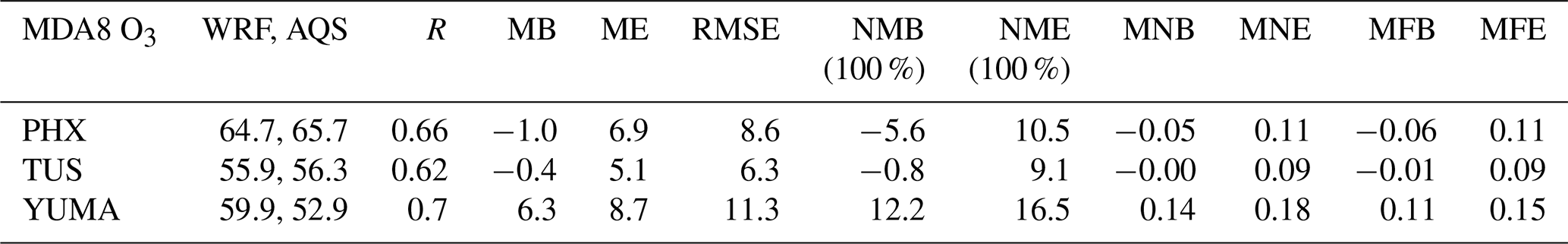
Overall, WRF-Chem MDA8 O3 exhibits a smaller mean bias compared to hourly O3, except at Yuma, where the mean bias slightly increases from 5.2 to 6.3 ppb. However, it is worth noting that the correlation coefficients show a slight decrease from 0.81 and 0.73 to 0.66 and 0.62 for PHX and TUS, respectively, compared to hourly O3. This reduction in correlation could be attributed to fewer data points available for linear fitting in the case of MDA8 O3. Additionally, the RMSE at PHX is reduced from 10.6 ppb for hourly O3 to 8.6 ppb for MDA8 O3. Considering statistics in both Tables 1 and 2, we conclude that WRF-Chem exhibits better performance in capturing the variations of MDA8 O3 concentrations than hourly O3.
Furthermore, when we compare WRF-Chem with CMAQ reanalysis, our findings indicate that WRF-Chem demonstrates smaller biases and higher correlations. For instance, the reanalysis consistently underestimates the MDA8 O3 at PHX but overestimates them at Yuma during the 4–9 June and 20–28 June periods, as illustrated in Fig. 4.
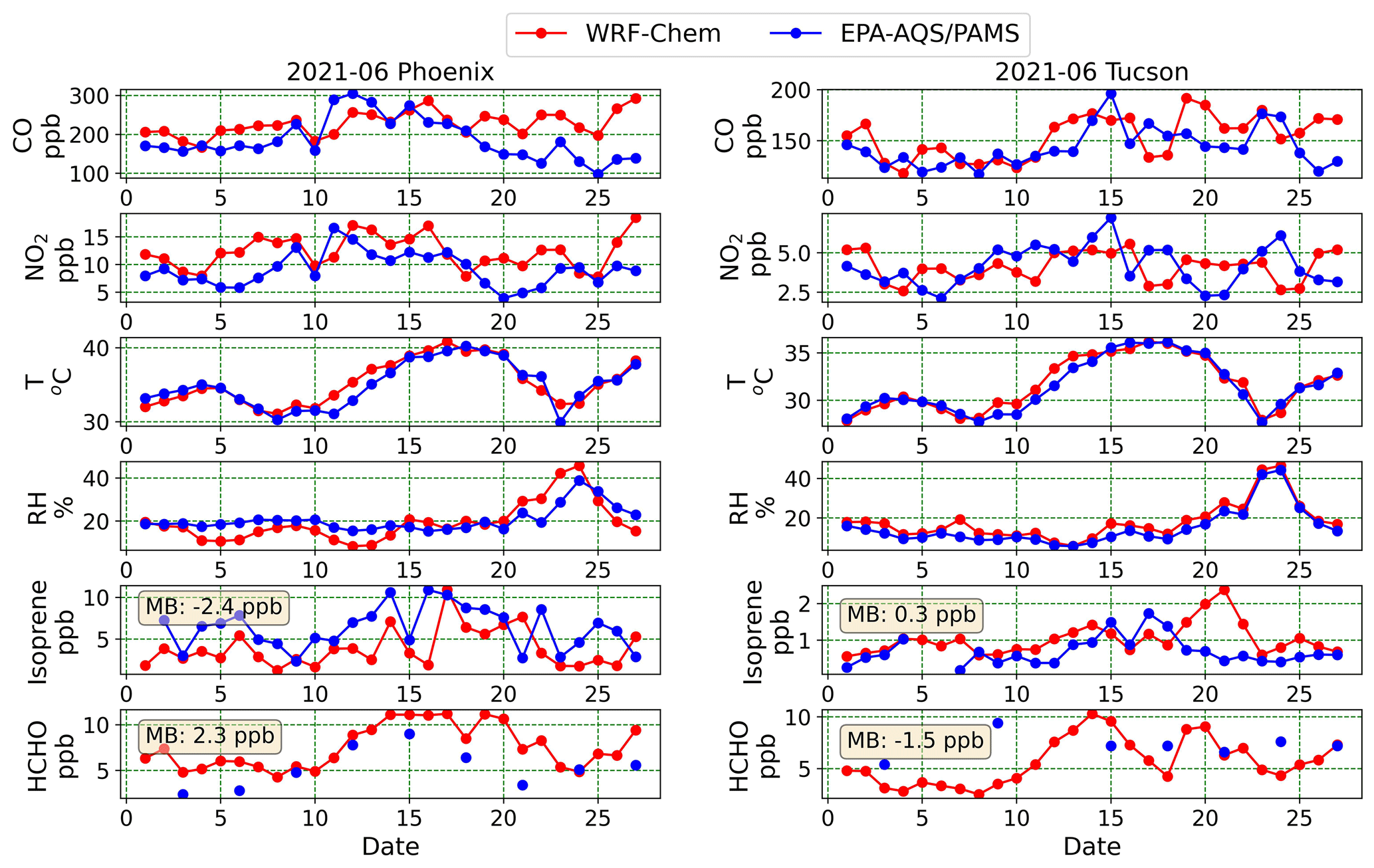
Figure 5WRF-Chem-simulated (red) and EPA-observed (blue) surface concentrations of CO and NO2, surface temperature (T), 2 m relative humidity (RH), surface concentrations of isoprene and formaldehyde (HCHO) for June 2021. CO, NO2, T, and RH measurements are obtained through the EPA AQS network. Isoprene and HCHO measurements are acquired from the EPA PAMS networks in PHX and TUS. The mean bias (MB) for isoprene and HCHO are also included.
Besides O3 evaluations, we examined other air pollutants and essential meteorological parameters. We present in Fig. 5 the daily surface concentrations of CO, NO2, isoprene, and formaldehyde (HCHO), along with surface T and RH, for June 2021. CO and NO2 are two prominent anthropogenic pollutants and serve as O3 precursors. Isoprene (the simplest five-carbon isoprenoid, C5H8) and monoterpene is the dominant BVOC emitted to the atmosphere and accounts for over 50 % of the total BVOC emissions (Guenther et al., 2012). Their concentrations are significantly influenced by factors such as temperature, vegetation, and light conditions (Morrison et al., 2016; Kalogridis et al., 2014). It is important to note that observations of VOCs using the PAMS system, in comparison to the well-established AQS monitoring system, remain relatively limited. Currently, the PAMS monitoring network in Arizona only operates during summer months from June to August and only started in recent years. For instance, of the two PAMS sites within Arizona, only two daily measurements of formaldehyde were recorded in June 2019 in Phoenix, and the observation schedule changed from 1 in 6 d to 1 in 3 d since 2018. In Tucson, formaldehyde observations only became available starting in 2021 with a 1 in 3 d schedule. Daily measurements of isoprene became available in both Phoenix and Tucson starting in 2021.
In comparison with the observations, the model appropriately replicated the daily variations of surface T and RH with minimal biases. However, for CO, WRF-Chem failed to capture the elevated episode over PHX during 11–15 June 2021. It is worth noting that during this period there was an active wildfire (Telegraph Fire, situated southeast of Phoenix, https://wfca.com/wildfire-articles/arizona-fire-season/, last access: 16 October 2023) that lasted 1 month and became one of the largest wildfires in the US throughout the 2021 wildfire season. Because of this, the CO levels in both Phoenix and Tucson were significantly impacted by the fire plumes with smoke moving right over Phoenix. The model may not be able to simulate the smoke plumes well. Despite the limited PAMS data, we were able to compare the daily isoprene concentrations with observations in both cities. On average, daily mean isoprene is around 5 ppb in PHX and 1 ppb in TUS. Furthermore, for HCHO concentrations, the model is comparable to the observations, not only in terms of the values, but also in capturing their variations. In conclusion, the online biogenic emission model employed in the WRF-Chem model, MEGAN 2.1, effectively simulates the BVOC levels.
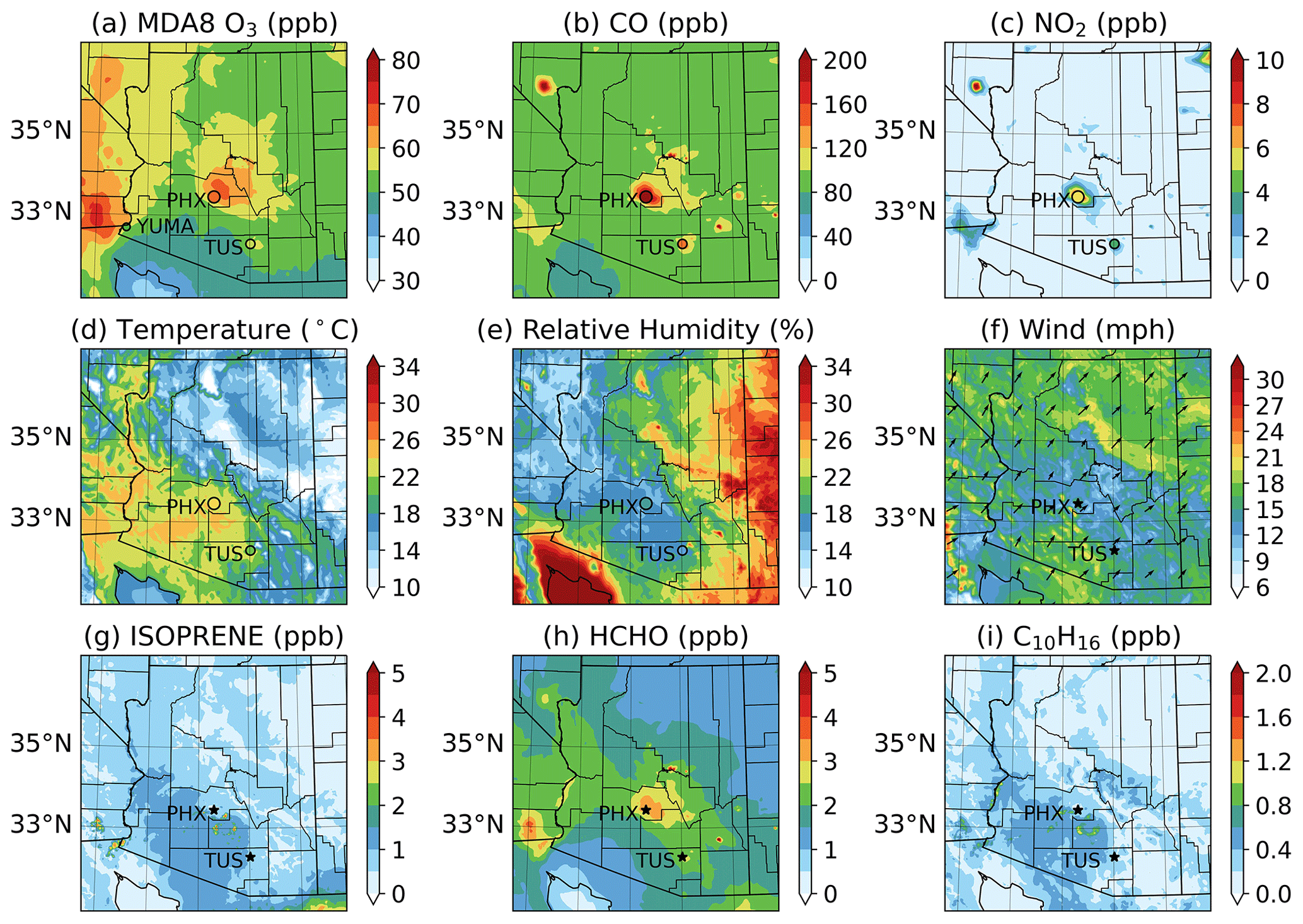
Figure 6WRF-Chem-simulated monthly mean concentrations of main pollution types (O3, CO, NO2), meteorological fields (temperature, relative humidity, wind), and major VOCs (isoprene, formaldehyde, and monoterpene). Colored circles represent the EPA AQS site observations for comparison.
Figure 6a–c presents the spatial plots of monthly mean surface concentrations of MDA8 O3, CO, and NO2 for June. The contour plots are based on hourly model output between the years 2017 and 2021. The colored circles represent the AQS surface observations for three cities: Phoenix (PHX), Tucson (TUS), and Yuma (YUMA). Both the WRF-Chem model and the observations indicate that MDA8 O3 in the Phoenix metro area reaches up to 65 ppb (Fig. 6a). The northeastern area of PHX, which is a downwind region, experiences significant O3 pollution as the prevailing winds in June are predominantly southwesterly winds (Fig. 6f). The background O3 level in most of Arizona is around 50 ppb, while western and southwestern Arizona, including Yuma, is substantially influenced by O3 from California.
For CO concentrations, the highest simulated surface levels in PHX reach 224.2 ppb, closely matching the corresponding AQS measurement of 221.9 ppb (Fig. 6b). Downwind of Phoenix, CO concentrations range between 100 and 120 ppb. Hotspots in the southeastern direction of both PHX and TUS are associated with wildfire burning events, such as the 2017 Frye Fire (southeastern hotspot of TUS) and the 2021 Telegraph Fire. The observed mean NO2 level in PHX is approximately 5 ppb and is mostly distributed in populated areas as the main source of NO2 is anthropogenic emissions. Figure S1 in the Supplement provides monthly mean O3, CO, and NO2 concentrations for individual years.
The aridity of southwestern Arizona is characterized by high temperatures and low RH. Shown in Fig. 6d–f are the mean surface temperature, 2 m RH, and surface winds. Notably, the temperature in PHX is slightly higher than that in TUS as PHX is located in the valley and TUS has a higher elevation (see Fig. 2b). The RH overall is under 20 % in southwestern Arizona, where the Sonoran Desert is located. The climate of the western and southwestern Arizona and other parts of Arizona is distinctive. The monthly mean wind predominantly comes from the southwesterly direction, with an average speed of around 4.5 m s−1 or 10 miles per hour (mph).
Table 3Statistics of WRF-Chem evaluation with respect to EPA AQS monitors. Results represent the average of June across 5 years between 2017 and 2021.
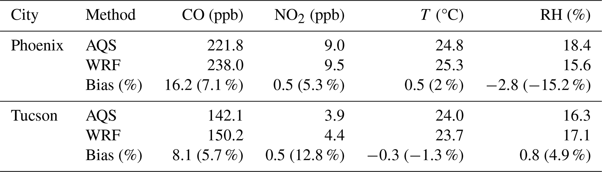
Table 3 presents the statistics of CO, NO2, T, and RH between simulations and observations for PHX and TUS. In general, the simulated values of O3, CO, and T (temperature) align well with the observations. Temperature shows a small, normalized bias of 2 % and −1.3 % for PHX and TUS, respectively. The model overestimates CO both in PHX and TUS by 7.1 % and 5.75 %, respectively. Additionally, the model overestimates the NO2 levels in both PHX and TUS. Figure 6g–i also demonstrates three dominant VOC concentrations: isoprene, formaldehyde (HCHO), and monoterpene (C10H16). Overall, the BVOCs are rather small over the desert region, except at Yuma, where it is largely impacted by agricultural vegetation.
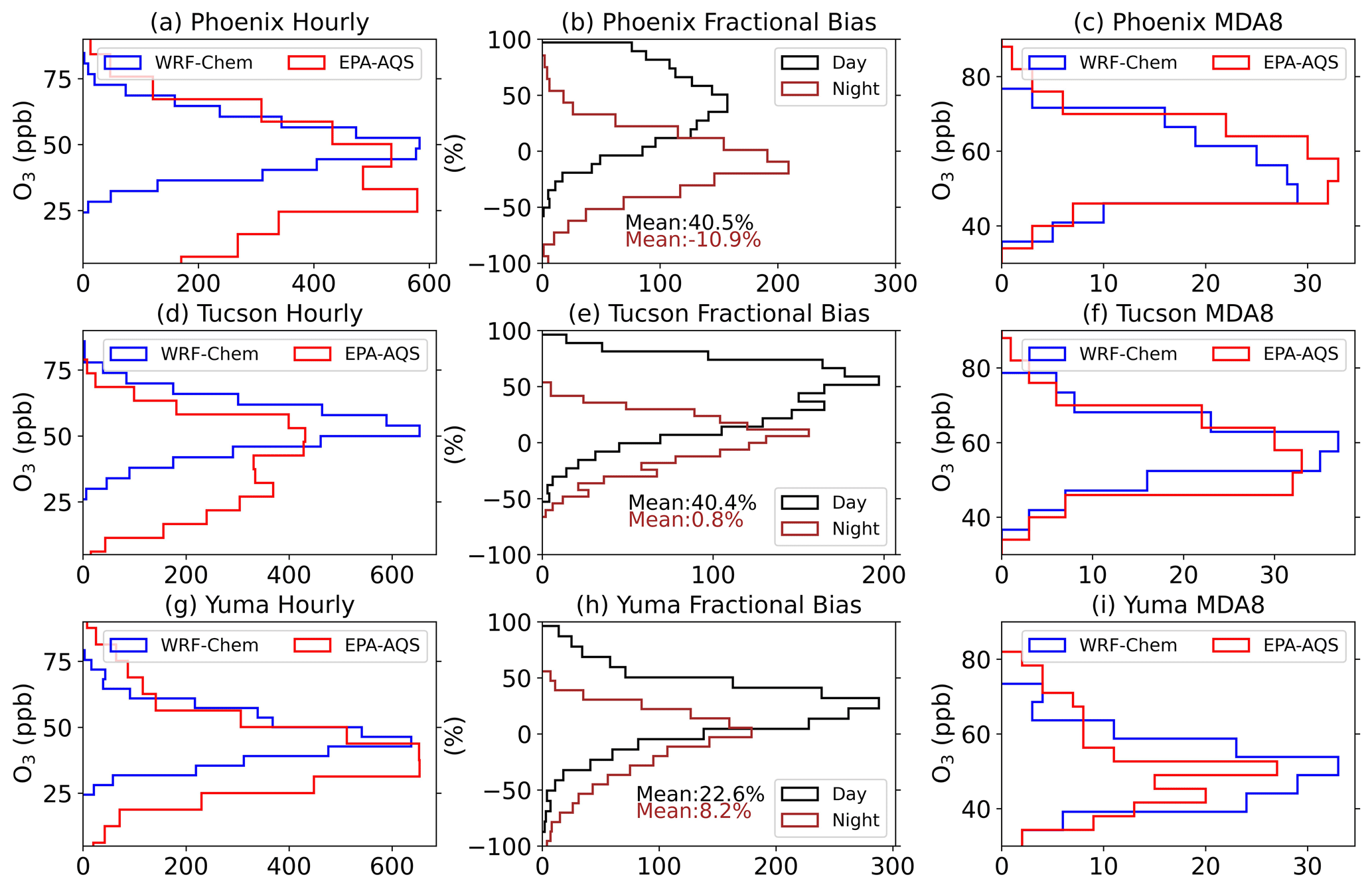
Figure 7Model evaluation for the cities of Phoenix (a–c), Tucson (d–f), and Yuma (g–i). The first panel in each row shows observed (red) and WRF-Chem-simulated (blue) surface O3 frequency distribution. The second panel is the frequency distribution of model bias for both daytime (black) and nighttime (brown). The third panel presents the frequency distribution of MDA8 O3.
To further investigate the bias between simulations and observations, in Fig. 7 we present the frequency distributions of hourly O3, the corresponding O3 bias with respect to the AQS observations, and MDA8 O3 for June in the 5-year period for Phoenix (top), Tucson (middle), and Yuma (bottom). For O3 levels higher than 50 ppb (background O3 level in Arizona), WRF-Chem demonstrates good performance in estimating the distributions in Phoenix and Yuma but tends to overestimate in Tucson, particularly between 50 to 60 ppb. Furthermore, WRF-Chem fails to capture the extremely high O3 observational days exceeding 70 ppb for all three cities. Conversely, for low O3 levels below 50 ppb, which are more associated with nighttime O3, WRF-Chem substantially underestimates the values. Therefore, for bias analysis, we divide the assessment into daytime and nighttime periods to account for the diurnal variability of O3 formation. The middle panel in Fig. 7 presents the fractional bias of hourly O3 between WRF-Chem and AQS observations. In general, during the daytime the mean bias is positive (Fig. 7b, e, h) suggesting an overestimation by WRF-Chem, while a negative mean bias during the night indicates that WRF-Chem underestimates the hourly O3 values in PHX. The MDA8 O3 distribution demonstrates better overall agreement between the model and observations than hourly O3, consistent with the statistics in Tables 1 and 2.
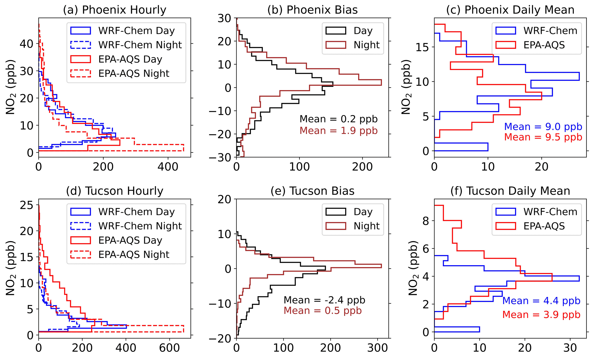
Figure 8The same as Fig. 7 but for surface NO2 concentrations at two cities: PHX (a–c) and TUS (d–f). The panels show, from left to right, hourly surface NO2 distributions, NO2 fractional bias, and daily mean NO2 distributions. Hourly NO2 distributions shown in the left panel are divided into daytime and nighttime.
To gain deeper insights into the factors contributing to O3 bias between daytime and nighttime, the distribution of surface NO2 concentration is presented in Fig. 8. For data quality purposes, surface NO2 concentrations that are less than 0.5 ppb are discarded for both simulations and observations. Similar to O3, the model misrepresents large NO2 episodes in PHX and TUS when NO2 is greater than 40 and 15 ppb, respectively. There is a larger diurnal variability in the observations than in simulations. The simulated NO2 distribution during daytime and night are comparable, while observed distributions are significantly different with distinct slopes (Fig. 8a, d). In PHX, the model overestimates the high NO2 levels (>10 ppb) during the night, while in TUS the model underestimates the NO2 during the daytime. The mean bias for day and night in PHX are 0.2 and 1.9 ppb, respectively. The mean bias for day and night in TUS is −2.4 and 0.5 ppb, respectively. The bias over Tucson suggests that WRF-Chem overestimates the NO2 during the night.
To address the biases depicted in Fig. 8 during daytime and nighttime, the PBLH is investigated. A higher PBLH allows pollutants and aerosols to disperse and mix with cleaner air over a larger vertical extent, resulting in a reduction of air pollutant concentrations. Consequently, an overestimation of PBLH leads to an underestimation of O3 and NO2, and conversely an underestimation of PBLH may contribute to overestimations of these pollutant levels. Using the radiosonde data, we estimated the PBLH at three cities and compared it with model simulations. The launching times of radiosondes at Arizona sites are at universal time (UT) hours of 12:00, 21:00, and 00:00, which correspond to local time (LT) hours of 05:00, 14:00, and 17:00, respectively.
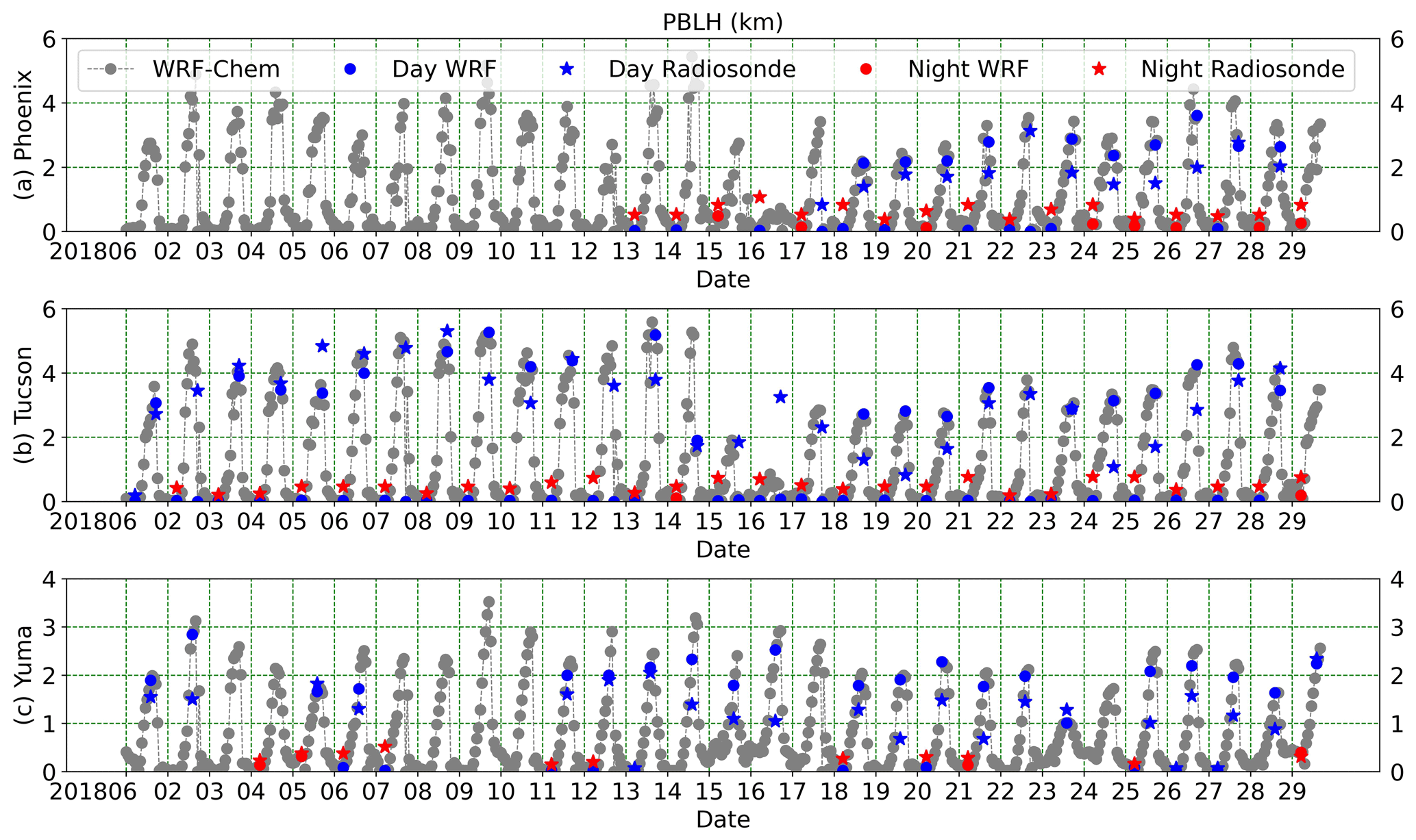
Figure 9Planetary boundary layer height (PBLH) in June 2018 for three cities: (a) Phoenix, (b) Tucson, and (c) Yuma. Dots and stars represent simulation from WRF-Chem and observation from radiosondes, respectively. Nighttime PBLH estimated from radiosonde data at 05:00 LT are denoted as red stars, with their corresponding simulated PBLH values indicated as red dots. Blue markers represent radiosondes launched during daytime with corresponding WRF-Chem simulations denoted by blue dots.
Presented in Fig. 9 are the PBLH for three cities, PHX, TUS, and YUMA, during June 2018 (additional years' data are available in the Supplement). The nighttime soundings launched at 05:00 LT are highlighted with red stars, and their corresponding WRF-Chem simulated PBLH values are represented as red dots. Conversely, daytime soundings are indicated by blue markers. Simulated PBLH at all other times without sounding data are labeled with grey dots. It is worth noting that the WRF-Chem model consistently demonstrates an underestimate of PBLH during nighttime (as denoted by the red markers) and an overestimate during daytime (as shown by the blue markers). The mean daytime bias of PBLH between model and observations at Phoenix (17:00 LT), Tucson (14:00 LT), and Yuma (14:00 LT) are 322.0, 18.1, and 602.5 m, respectively. These biases are closely related to the MDA8 O3 bias listed in Table 2 where bias in Phoenix is larger than Tucson. The nighttime biases are all negative with values of −509.7, −435.4, −55.8 m, indicating an overall underestimate. The underestimate of PBLH during the night will cause the shallower vertical mixing of daytime accumulated O3 leading to the positive bias of nighttime O3 observed in Fig. 7.
3.1.1 O3 exceedance
According to the EPA, an exceedance day occurs on each calendar day when the MDA8 O3 concentration is greater than 70 ppb, where 70 ppb is the ground-level O3 standard from the 2015 National Ambient Air Quality Standards (NAAQS). A design value, on the other hand, is a statistic that describes the air quality status of a given location relative to the NAAQS level. The O3 design value of the Phoenix–Mesa metropolitan area has increased from 76 ppb in 2017 to 81 ppb in 2022 (refer to Table S1). The rising and persisting O3 levels led to the reclassification of Phoenix–Mesa metropolitan area from a marginal to a moderate non-attainment status for O3 limits by the EPA. In the previous section, we demonstrated that WRF-Chem exhibits good performance in simulating the mean O3 and other precursor parameters. Moreover, the model performs better with the MDA8 O3. To further investigate the issue of O3 pollution in Phoenix, this section focuses on O3 exceedances. As depicted in Fig. 1, O3 exceedances typically first start in April and finally occur in September, with the exception of the year 2019 when exceedances extended into October and the year 2021 when no exceedance was observed in April. Over the 5-year period from 2017 to 2021, in the greater Phoenix area the average annual count of O3 exceedance days was 43. Even in 2020, amidst the onset of the COVID-19 pandemic and the enforcement of stay-at-home measures, which resulted in reduced concentrations of NOx, O3 exceedances in Phoenix did not exhibit significant reduction. Figure 10c illustrates the boundary of the designated Maricopa County non-attainment area (NAA, depicted by polygons outlined in black), along with the locations of AQS sites equipped for O3 monitoring. In total, there are 29 monitoring sites, with 27 of them situated within the NAA boundary.
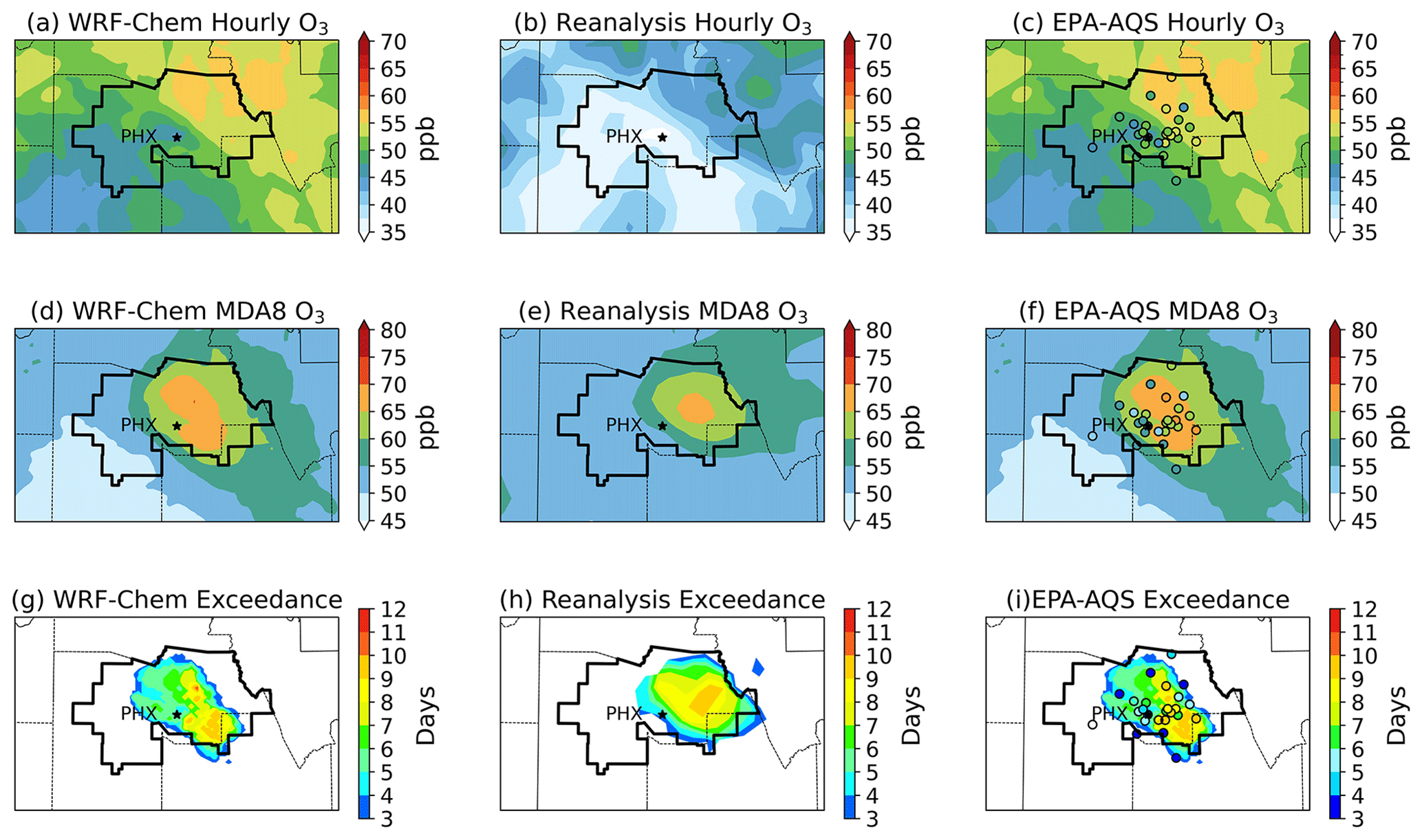
Figure 10Comparison of WRF-Chem simulation (a, d, g), CMAQ reanalysis (b, e, h), and EPA AQS observations (colored circles) overlaid with WRF-Chem results (c, f, i) depicting monthly mean surface hourly and MDA8 O3 concentrations (a–f) and exceedance days (g–i) in June 2017. O3 exceedance is defined as a day when the MDA8 concentration exceeds 70 ppb. The Phoenix–Mesa non-attainment area is bounded by black curves.
Presented in Fig. 10 are the spatial variations of the mean O3, MDA8 O3, and count of O3 exceedance days for June 2017 within the Maricopa County NAA. In the top row (Fig. 10a–c), we depict the monthly mean surface hourly O3 concentrations as derived from WRF-Chem, CMAQ reanalysis, and data from AQS monitor sites. These 27 AQS sites, encompassing a range of urbanization levels, population densities, and downwind/upwind positions, exhibit considerable variability even within the NAA. Figure 10d–f show the monthly mean MDA8 O3 concentrations, with higher levels observed in the northeastern part of the NAA, a pattern accurately captured by both WRF-Chem and the reanalysis. Better agreement among model and observations is evident considering both hourly and MDA8 O3. The reanalysis data substantially underestimates the mean hourly O3 levels by 10 ppb but captures the MDA8 O3 spatial distribution pattern. Lastly, the count of O3 exceedance days is shown in Fig. 10g–i. The exceedance days vary from 2 to 10 d within the area. The regions with the highest population density, particularly the central Phoenix–Mesa region, exhibit the highest counts of exceedance days. Additionally, since the prevailing wind in June is westerly (Figs. 1 and 6), the east side of the valley is observed with higher O3 levels. In general, the model exhibits strong agreement with the observational data regarding factors such as location, number of days, spatial extent, and spatial variability.
3.2 O3 source attribution
Source attribution of O3 is challenging due to the complex processes that control O3 formation. Tropospheric O3 levels are influenced by a multitude of factors including (1) meteorological factors, such as T, RH, cloud cover, radiation, wind speed and direction, precipitation, and boundary layer height; (2) O3 precursors, such as NOx, VOCs, and CO, which can originate from biomass burning (wildfire, prescribed fire), biogenic emissions, and anthropogenic emissions; and (3) O3 transport, such as long-range transport and stratospheric O3 intrusions. Understanding the relationships between these factors and O3 levels is essential for discerning their respective impacts on ambient O3 concentrations. Several analytical methods are available for investigating O3 source attributions, e.g., backward trajectory analysis (Xiong and Du, 2020; Dimitriou and Kassomenos, 2015; Betito et al., 2024), machine learning algorithms (Cheng et al., 2023; Mishra et al., 2023; Weng et al., 2022), and chemistry models (Butler et al., 2020; Lupaşcu and Butler, 2019; Sudo and Akimoto, 2007). In this paper, we employ scatter plots that utilize both model outputs and ground observations. These scatter plots serve as a practical means to delve deeper into the intricate connections between O3 and its major influencing factors, aiding in the identification and quantification of their contributions to O3 concentrations in the atmosphere.
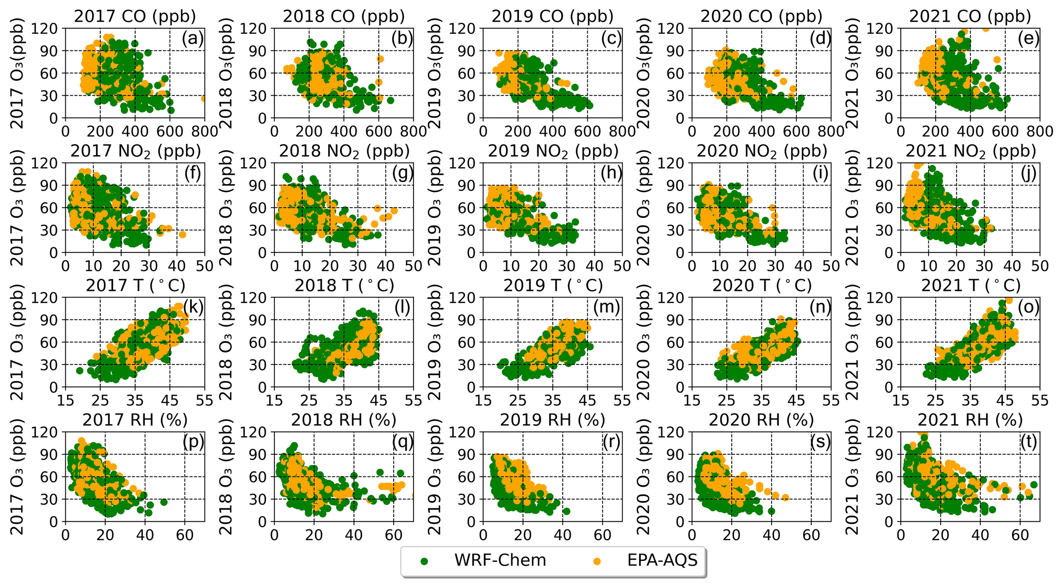
Figure 11WRF-Chem-simulated (green) and EPA AQS (orange) hourly CO, NO2, surface temperature (T), and relative humidity (RH) versus hourly O3 concentration during the daytime.
Figure 11 presents a series of scatter plots that illustrate the relationships between O3 concentrations and other key variables, including CO, NO2, surface T, and RH during daylight hours at the Phoenix JLG Supersite. The data points are color coded, with green denoting simulations and orange representing observations. Each column panel within the figure corresponds to the respective month of June for individual years spanning from 2017 to 2021. The displacement between the orange and green dots on the first row suggests that WRF-Chem overestimates the CO concentrations in all the years except 2018. In the years 2017 and 2021, more extreme O3 concentrations were present with levels exceeding 100 ppb.
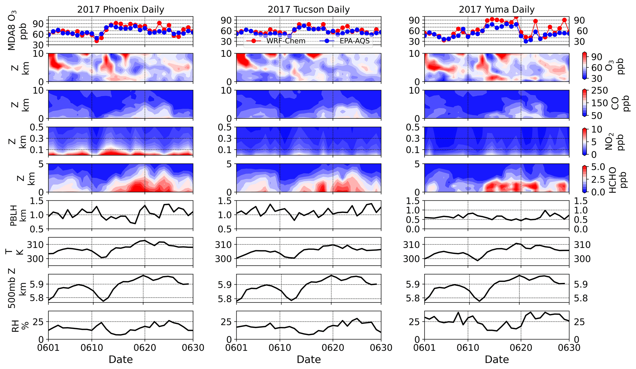
Figure 12Vertical profiles of simulated O3, CO, NO2, and HCHO at three cities (contour plots) along with the surface MDA8 O3 (top panel), PBLH, surface temperature (T), 500 mb height, and surface relative humidity (RH) in June 2017. An O3 exceedance event on 13 June was observed in all three cities.
The negative correlation between NO2 and O3 (depicted in Fig. 11f–j) reveals that in Phoenix surface O3 levels tend to be higher when NO2 concentrations are lower. When hourly NO2 levels exceed 25 ppb, O3 concentrations generally remain below 60 ppb. Furthermore, the positive correlation between temperature and O3 suggests that in general elevated temperatures are associated with higher O3 levels. It is worth noting that on some extreme hot days, O3 levels can also be low. Conversely, the negative correlation between RH and O3 indicates that increased RH tends to be linked with lower O3 concentrations. These intricate relationships offer valuable insights into the complex interplay between O3 and its influencing factors within the Phoenix JLG Supersite region.
As previously discussed in earlier sections, the O3 exceedance in Arizona originates from a combination of various contributing factors, which can be classified into two main categories: local production and transport. Notably, on 13 June 2017, the observed surface O3 levels in both Phoenix and Yuma experienced a substantial increase, with a MDA8 concentration of approximately 90 ppb in Phoenix. This particular event has been successfully captured by both the WRF-Chem model and CMAQ reanalysis, as illustrated in Fig. 4. Shown in Fig. 12 are the simulated vertical profiles of O3, CO, NO2, and HCHO, as well as the surface meteorological parameters, including PBLH, temperature (T), 500 mb height, and RH, during this extreme event. The simulated and AQS observed MDA8 O3 are also included for reference. During the event, both the surface and columnar concentrations of CO, NO2, and HCHO were all elevated, particularly in the boundary layer. In the meantime, PBLH and RH decreased, while temperature and 500 mb height increased, consistent with the correlation relationships observed in Fig. 11. Furthermore, we employed the Hybrid Single-Particle Lagrangian Integrated Trajectory model (HYSPLIT) (Rolph et al., 2017; Stein et al., 2015) to calculate 48 h back trajectories for the 13 June exceedance event, as illustrated in Fig. S5. As depicted in Fig. 12, at the onset of the extreme events on 13 June 2017, temperatures were lower compared to previous days. However, as the event progressed, a heat episode emerged over Phoenix following a decrease in PBLH. The 48 h back trajectories suggest a potential influence in air masses (O3 or its precursors) originating from California or Asia contributing to the elevated O3 levels observed in Phoenix on 13 June 2017. Subsequently, in the following days, the high O3 concentrations are more associated with local production.
3.3 O3-NOx-VOC sensitivity
The O3-NOx-VOC sensitivity is a crucial concept in the fields of atmospheric chemistry and air quality management (Duncan et al., 2010; Sillman, 1995; Sillman and He, 2002; Sillman et al., 2003; Liu and Shi, 2021; Carrillo-Torres et al., 2017; Zaveri et al., 2003). It refers to how the concentration of O3 in the atmosphere responds to changes in the levels of NOx and VOCs. Understanding this sensitivity is essential for assessing and managing air quality, particularly in regions where O3 pollution is a concern. The sensitivity is often quantified as the ratio of VOC to NOx, an important parameter for characterizing the efficiency of O3 formation in the environment. When this ratio is high, O3 formation is constrained primarily by the availability of NOx, leading to what is defined as NOx-limited or NOx-sensitive chemistry. Consequently, taking measures to reduce NOx emissions directly correlates with O3 reduction. Conversely, under lower ratios, it is referred to as a VOC-limited or VOC-sensitive regime. In these scenarios, O3 levels are notably more responsive to reductions in VOCs, and solely decreasing NOx may not effectively lower O3 concentrations and even worse may increase O3 levels. Ratios between the two regimes are considered transitional, and both NOx and VOC controls may be effective.
However, it is important to acknowledge that the specific range of ratios used to define VOC and NOx limitations can vary among researchers and depend on the specific dataset and variables under consideration. Different studies and regulatory assessments may employ distinct criteria for categorizing O3 sensitivity to VOCs and NOx, making it imperative to consider these variations when interpreting and applying sensitivity analyses in different contexts. From an observational perspective, the HCHO concentration has been widely used as a proxy for VOC reactivity as it is a short-lived oxidation product of many VOCs and positively correlated with peroxyl radicals (Sillman, 1995), and it is also available in many observational datasets. The concentration of HCHO serves as an indicator for volatile organic compound (VOC) reactivity as it exhibits a positive correlation with proxy radicals (Sillman, 1995). Sillman (1995) identified that elevated ratios typically indicate NOx-limited regimes, whereas reduced ratios are indicative of VOC-limited regimes. Satellite data, like TROPOMI (The Tropospheric Monitoring Instrument), provide daily columnar HCHO and NO2 spatial distributions at a certain time of the day. Thus, satellite data have been widely used in determining the VOC-NOx sensitivity regimes (Duncan et al., 2010; Souri et al., 2020; Jin et al., 2017; Martin et al., 2004). In this study, we also employ the HCHO-to-NO2 ratio (FNR) as a proxy for assessing VOC-NOx sensitivity. Surface FNRs are usually lower by considering surface or planetary boundary layer number concentrations since the vertical distribution of HCHO and NO2 varies as shown in Fig. 12. HCHO is distributed up to 5 km, whereas NO2 predominantly remains within 0.5 km. Various studies have investigated the FNR threshold for regime determination. Schroeder et al. (2017) defined the transitional regime with FNR values ranging from 0.7 to 2.3, while Duncan et al. (2010) reported a range of 1.0 to 2.0, and Jin et al. (2020) found values of 3.2 to 4.1 using satellite column retrievals. Additionally, Acdan et al. (2023) utilized ground-based PAMS measurements and proposed an FNR range of 0.3 to 1.0 for the transition over the Lake Michigan region.In our study, we follow Duncan et al. (2010), who linked the FNR with surface O3 with model simulation, and their sensitivity regime definition has been used in several studies (Tang et al., 2012; Jin and Holloway, 2015; Souri et al., 2017) by Duncan et al. (2010). When FNR is less than 1, it is classified as VOC-limited; when it falls between 1 and 2, it is considered a transitional regime; and when FNR exceeds 2, it is defined as NOx-limited.
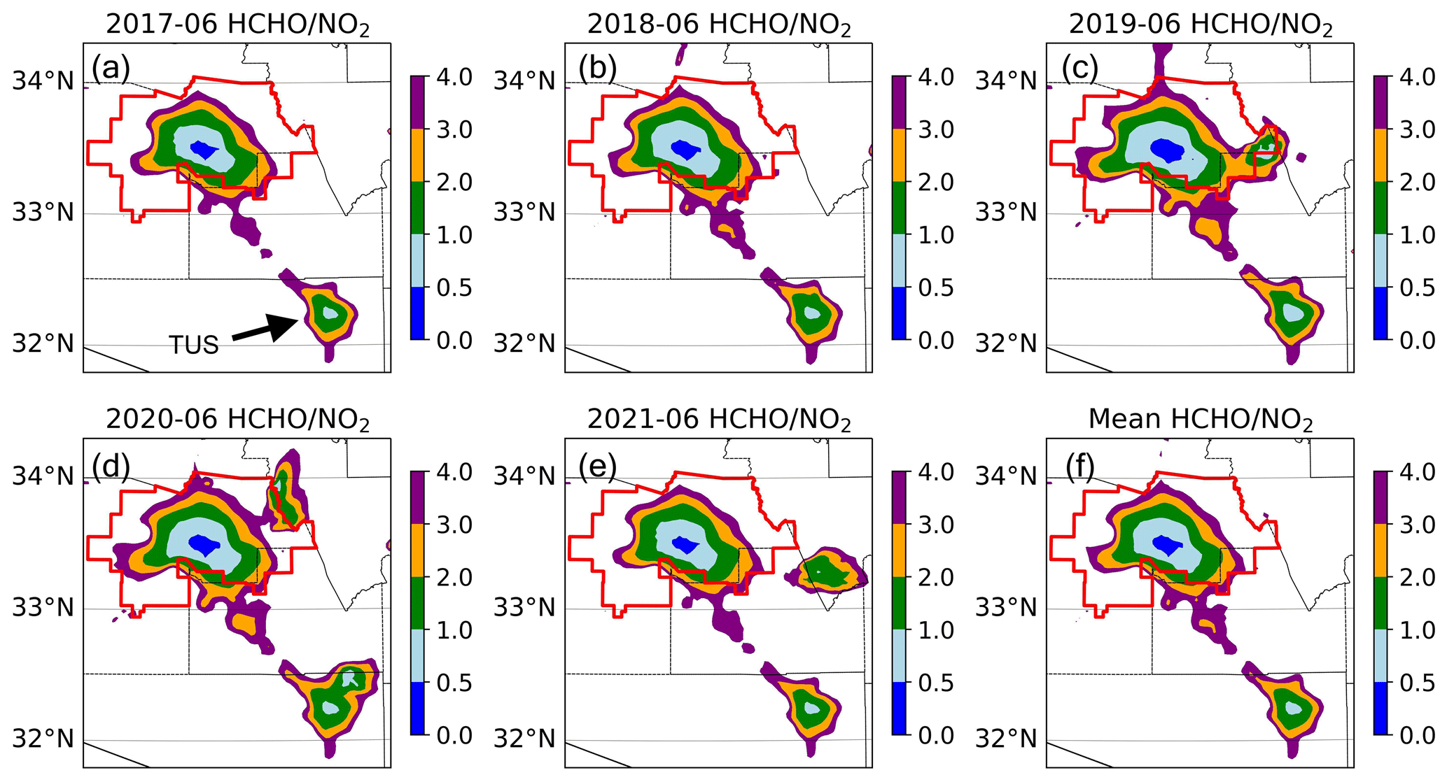
Figure 13WRF-Chem-simulated monthly mean ratio of surface over Phoenix and Tucson. Red lines represent the non-attainment area designated by the EPA. “WF” denotes instances of “pop-up” low FNRs resulting from wildfire events.
In the previous section, we demonstrated a negative correlation between NO2 and O3, indicating that Phoenix falls within the VOC-limited or VOC-sensitive regime. To gain a more comprehensive understanding of NOx-VOC sensitivity in the greater Phoenix metropolitan area, we calculated monthly FNR values for each year and their respective means. Figure 13 displays spatial maps of FNR across Phoenix and Tucson, highlighting grids with FNR values less than or equal to 4. The Maricopa County non-attainment area (NAA) is outlined in red. Overall, central Phoenix is predominantly characterized as a VOC-limited or transitional regime, with FNR values consistently below 2 and an average FNR of 1.15 across the metropolitan area. The FNR tends to be lower within the more densely populated urban areas. As one moves towards the suburban areas, there is an increase in FNR, marking a transition from the VOC-limited regime to the boundary between VOC-limited and NOx-limited conditions. Additionally, Phoenix exhibits lower FNR values compared to Tucson. Notably, hotspots related to fire activities are evident in different years, such as the eastern region of Phoenix in 2019, the northeastern areas of Phoenix and Tucson in 2020, and the eastern part of Phoenix in 2021. Fire and biomass burning activities typically result in significant emissions of CO, CO2, NOx, VOCs, particulate matter, methane, and more. Consequently, when these fire events occur, they can alter the NOx-VOC sensitivity of the affected areas. The “pop-up” local FNR minima in Fig. 13 (labeled as WF) suggests that wildfire events lead to a reduction in the FNR and a shift in the sensitivity regime towards VOC-limited. Similar results have been reported using satellite observations, where they found that during the fire event, the NOx values are high near the fire leading to lower FNRs. The varying contours from year to year indicate slight differences in sensitivities between those years, with 2019 and 2020 showing lower mean FNR values over the NAA compared to other years.
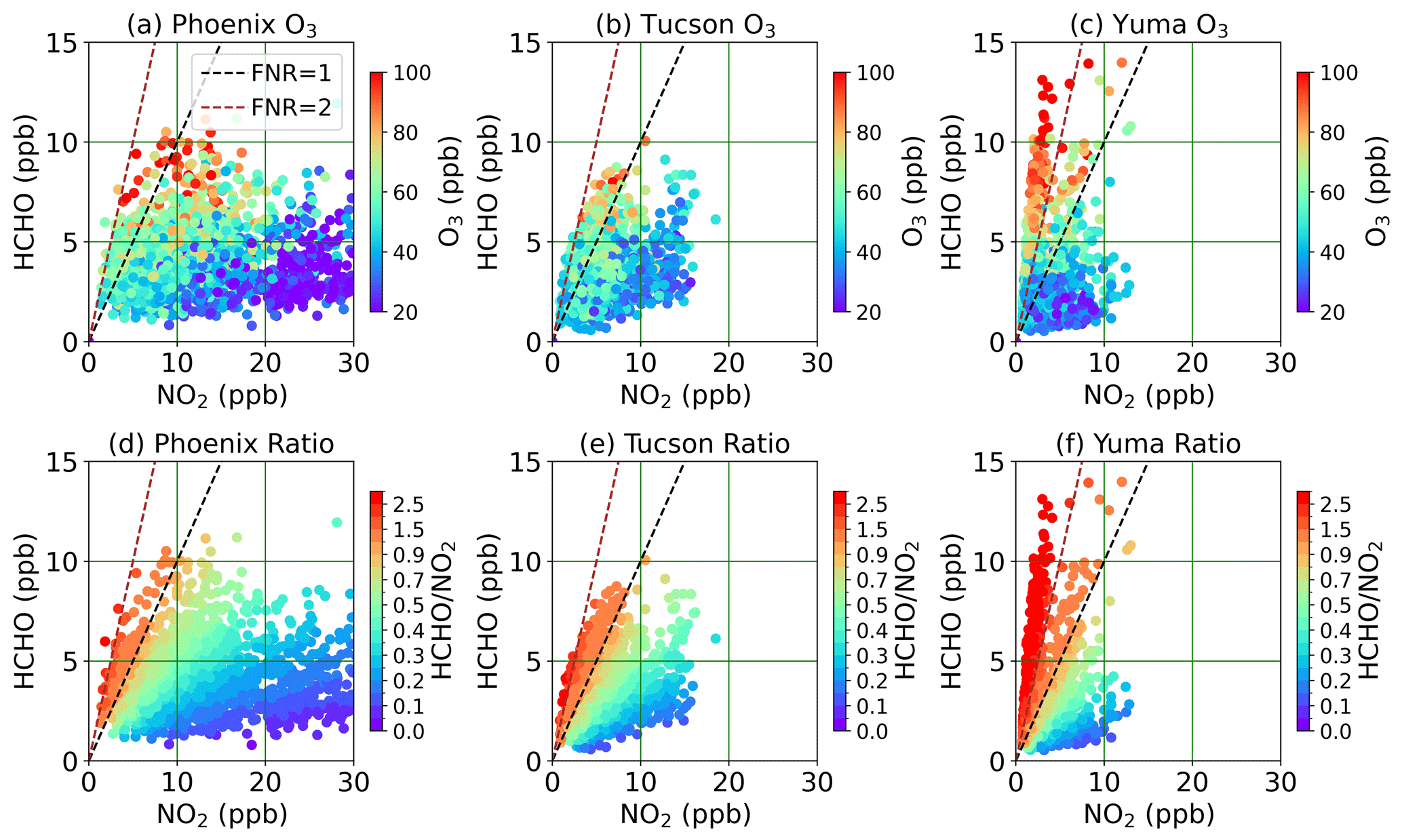
Figure 14Scatter plots of WRF-Chem simulated hourly surface NO2 versus HCHO concentrations at three cities: Phoenix, Tucson, Yuma. The colors represent the corresponding O3 concentrations (a–c) and ratio of (FNR; d–f) for years from 2017 to 2021. Dashed black and brown lines represent the FNR values of 1 and 2, respectively.
In Fig. 14, we present scatter plots illustrating the relationship between hourly surface concentrations of NO2 and HCHO in three cities: Phoenix, Tucson, and Yuma, as simulated by WRF-Chem. The color gradients in these scatter plots correspond to the respective O3 concentrations (panels a–c) and FNR values (panels d–f).
When we compare Fig. 14a with 14d, in Phoenix we observe that elevated O3 concentrations are linked to lower NO2 levels (as also seen in Fig. 11) and high HCHO concentrations, falling within the range of 0.5 to 1.2 in terms of FNR. Conversely, the lowest O3 levels occur when NO2 levels are relatively high. In Tucson, NO2 levels are approximately half of those observed in Phoenix, and O3 occurrences are less frequent. Higher O3 concentrations in Tucson are primarily associated with FNR values greater than 1. Yuma, on the other hand, exhibits the lowest levels of NO2, but it has the highest HCHO concentrations, which are also accompanied by high O3 levels. Notably, the mean FNR in Yuma is also the highest among the three cities, as indicated by the prominent red color in Fig. 14f.
Understanding these correlations between HCHO, NO2, and O3 levels is crucial for formulating effective regulatory strategies aimed at mitigating O3 pollution in urban settings resulting from localized O3 production. The transitional regime observed in the Phoenix metropolitan area suggests that while additional reductions in NO2 levels could potentially decrease O3 design values, there exists the possibility of concurrent increases in daily mean O3 levels due to the intricate interplay of diurnal complex O3 production. In Yuma, where higher HCHO levels prevail, reducing VOC emissions may serve as a viable approach to lowering O3 concentrations.
In this study, our primary objective was to gain a comprehensive understanding of surface O3 pollution in an arid and semi-arid climate region, with a specific focus on the state of Arizona as a representative case study. To achieve this, we employed WRF-Chem simulations to simulate O3 and various other gases, examining the month of June within a 5-year period spanning from 2017 to 2021. Our model's performance was assessed by comparison with surface observations from the EPA AQS and PAMS monitoring networks, as well as a CMAQ reanalysis product. Our analysis primarily focused on three major cities within Arizona: Phoenix, Tucson, and Yuma. We calculated statistics for both hourly and MDA8 O3 concentrations. We also examined additional monthly mean fields, including key meteorological parameters (T, RH, wind) and air pollutants (NO2, CO, VOCs). Results show that WRF-Chem demonstrated better performance in simulating MDA8 O3 compared to hourly O3. The model exhibited a tendency to overestimate nighttime NO2 levels, resulting in larger biases during the night; the model also shows an overestimate of surface NO2 in Phoenix and an underestimate of NO2 in Tucson. Among the cities examined, Yuma displayed the highest mean error and a positive bias, whereas Phoenix and Tucson showed closer agreement with observations, featuring smaller errors and negative biases. Furthermore, our evaluation indicated minimal biases in the representation of meteorological parameters. However, for VOCs, the model underestimated their surface concentrations.
O3 exceedances were also investigated and evaluated at all available AQS monitoring sites in Maricopa County. Our model exhibited strong agreement with site measurements regarding both the magnitude and the number of days on which an O3 exceedance occurred considering factors such as location, number of days, spatial extent, and spatial variability. The analysis of an O3 exceedance case beginning on 13 June 2017, along with the back trajectories, suggests that Arizona can also be affected by long-range transport from interstate or continental sources.
To better understand the O3 formation in this arid and semi-arid region, we examined the correlation between O3 and other factors influencing O3 production. In Phoenix, the scatter plots exhibited overall negative correlations between O3 and CO, NO2, and RH, while positive correlations were strongly observed with T and HCHO. These correlations suggest that O3 levels are higher when NO2 concentrations are generally lower and HCHO concentrations are higher, indicating that central Phoenix falls within the VOC-limited regime. Additionally, our spatial maps of the FNR confirm that in the most densely populated urban areas, the region predominantly falls within the VOC-limited regime, with FNR less than 1. Moving outward from this area the FNR values increase, indicating a shift to a transitional and NOx-limited regime. This analysis significantly contributes to our understanding of O3 dynamics in arid and semi-arid regions and has implications for air quality management and policy in such environments.
In terms of the uncertainties associated with the approaches in this study, they are largely dependent on the bias and uncertainty inherent in the emissions data used for our model simulations. In the case of anthropogenic emissions, our utilization of NEI2017 data for years other than the reference year introduces potential errors due to variations in emissions over time. This particularly affects the representation of precursor pollutants, notably NOx. Moreover, the underestimation of HCHO and other biogenic emissions simulated from MEGAN 2.1 may also contribute to a negative bias in the FNR, leading to the bias in regime determination. Additionally, dust events are particularly common in Arizona, especially in the southwestern region where the Sonora Desert is situated. The presence of dust can significantly impact ozone photolysis dynamics by interacting with sunlight. Dust particles can scatter and absorb solar radiation, thereby altering the photolysis rates of ozone molecules in the atmosphere. Consequently, these events may introduce bias to our findings. However, according to Lader et al. (2016) and Ardon-Dryer et al. (2023), dust storm events are most frequent during the monsoon season (in July and August), typically peaking around 18:00–19:00 LT, when photolysis rates are at their lowest. Focusing on the dry summer month of June in this study helps alleviate the bias caused by these dust events.
However, a better performance of the model can be pursued through various strategies. While achieving a higher spatial resolution, such as 1 km, is desirable, it remains constrained by the available computational resources and the resolution of input datasets, for instance, the NEI currently operating at 4 km resolution. A potential remedy involves employing a finer-resolution emission dataset, such as the Neighborhood Emission Mapping Operation (NEMO) proposed by Ma and Tong (2022). Additionally, refining simulations of nighttime chemistry, crucial for accurate predictions, necessitates a more precise estimation of the PBLH, which, if improved, can contribute to reducing the O3 bias during nocturnal hours. This improvement can be achieved by assimilating PBLH estimates obtained from radiosonde and ceilometer data.
For future work, we aim to continue investigating the contributions of individual sources of O3 to total O3 levels. We will adopt a tagging technique developed by Emmons et al. (2012) and Butler et al. (2018). This tagging technique uses the WRF-Chem model with the MOZART gas chemistry mechanism to attribute the sources contributing to tropospheric O3. We will focus on the contributions from anthropogenic, fire, and biogenic emissions and also use the model to trace the transport of O3 and its precursors (NOx, VOC) from their source.
The WRF-Chem model is version 4.4 is available for download from Zenodo (https://doi.org/10.5281/zenodo.10479471, Guo, 2024) and publicly available at NCAR https://www2.mmm.ucar.edu/wrf/users/download/get_source.html (last access: 25 June 2022). The model outputs, ADEQ forecast, and CMAQ reanalysis datasets can be provided upon request to the corresponding author. EPA AQS and PAMS hourly and daily datasets are available at https://aqs.epa.gov/aqsweb/airdata/download_files.html (EPA, 2023b).
The supplement related to this article is available online at: https://doi.org/10.5194/gmd-17-4331-2024-supplement.
YG and AFA designed the research. YG performed the model runs and subsequent analysis. YG wrote the paper with contributions from AFA and AS. RK provided the reanalysis dataset. MAM and CR helped with the observational data acquisition and preprocessing.
The contact author has declared that none of the authors has any competing interests.
Publisher's note: Copernicus Publications remains neutral with regard to jurisdictional claims made in the text, published maps, institutional affiliations, or any other geographical representation in this paper. While Copernicus Publications makes every effort to include appropriate place names, the final responsibility lies with the authors.
We especially acknowledge Gabriele Pfister (NCAR/ACOM) and Rajesh Kumar (NCAR/RAL) for kindly providing the NCAR WRF-Chem forecasting and reanalysis system configurations, for which this study is being built upon. We also thank Matthew Pace and Michael Graves at the Arizona Department of Environmental Quality (ADEQ) for providing their forecasts for the state of Arizona. The authors also gratefully acknowledge the NOAA Air Resources Laboratory (ARL) for the provision of the HYSPLIT transport and dispersion model and READY website (https://www.ready.noaa.gov, last access: 1 November 2023) used in this publication.
This work is supported by an Arizona Board of Regents (ABOR) Regent's Grant from the Technology and Research Initiative Fund (TRIF).
This paper was edited by Jason Williams and reviewed by three anonymous referees.
Acdan, J. J. M., Pierce, R. B., Dickens, A. F., Adelman, Z., and Nergui, T.: Examining TROPOMI formaldehyde to nitrogen dioxide ratios in the Lake Michigan region: implications for ozone exceedances, Atmos. Chem. Phys., 23, 7867–7885, https://doi.org/10.5194/acp-23-7867-2023, 2023.
Achakulwisut, P., Anenberg, S. C., Neumann, J. E., Penn, S. L., Weiss, N., Crimmins, A., Fann, N., Martinich, J., Roman, H., and Mickley, L. J.: Effects of Increasing Aridity on Ambient Dust and Public Health in the U.S. Southwest Under Climate Change, GeoHealth, 3, 127–144, https://doi.org/10.1029/2019GH000187, 2019.
Anderson, H. R.: Air pollution and mortality: A history, Atmos. Environ., 43, 142–152, https://doi.org/10.1016/j.atmosenv.2008.09.026, 2009.
Ardon-Dryer, K., Gill, T. E., and Tong, D. Q.: When a Dust Storm Is Not a Dust Storm: Reliability of Dust Records From the Storm Events Database and Implications for Geohealth Applications, Geohealth, 7, e2022GH000699, https://doi.org/10.1029/2022gh000699, 2023.
Asadi Zarch, M. A., Sivakumar, B., Malekinezhad, H., and Sharma, A.: Future aridity under conditions of global climate change, J. Hydrol., 554, 451–469, https://doi.org/10.1016/j.jhydrol.2017.08.043, 2017.
Betito, G., Arellano, A., and Sorooshian, A.: Influence of Transboundary Pollution on the Variability of Surface Ozone Concentrations in the Desert Southwest of the U.S.: Case Study for Arizona, Atmosphere, 15, 401, https://doi.org/10.3390/atmos15040401, 2024.
Butler, T., Lupascu, A., Coates, J., and Zhu, S.: TOAST 1.0: Tropospheric Ozone Attribution of Sources with Tagging for CESM 1.2.2, Geosci. Model Dev., 11, 2825–2840, https://doi.org/10.5194/gmd-11-2825-2018, 2018.
Butler, T., Lupascu, A., and Nalam, A.: Attribution of ground-level ozone to anthropogenic and natural sources of nitrogen oxides and reactive carbon in a global chemical transport model, Atmos. Chem. Phys., 20, 10707–10731, https://doi.org/10.5194/acp-20-10707-2020, 2020.
Carrillo-Torres, E. R., Hernández-Paniagua, I. Y., and Mendoza, A.: Use of Combined Observational- and Model-Derived Photochemical Indicators to Assess the O3-NOx-VOC System Sensitivity in Urban Areas, Atmosphere, 8, 22, https://doi.org/10.3390/atmos8020022, 2017.
Cheng, Y., Huang, X.-F., Peng, Y., Tang, M.-X., Zhu, B., Xia, S.-Y., and He, L.-Y.: A novel machine learning method for evaluating the impact of emission sources on ozone formation, Environ. Pollut., 316, 120685, https://doi.org/10.1016/j.envpol.2022.120685, 2023.
Chin, M., Ginoux, P., Kinne, S., Torres, O., Holben, B. N., Duncan, B. N., Martin, R. V., Logan, J. A., Higurashi, A., and Nakajima, T.: Tropospheric Aerosol Optical Thickness from the GOCART Model and Comparisons with Satellite and Sun Photometer Measurements, J. Atmos. Sci., 59, 461–483, https://doi.org/10.1175/1520-0469(2002)059<0461:TAOTFT>2.0.CO;2, 2002.
Cooper, O. R., Gao, R.-S., Tarasick, D., Leblanc, T., and Sweeney, C.: Long-term ozone trends at rural ozone monitoring sites across the United States, 1990–2010, J. Geophys. Res.-Atmos., 117, D22307, https://doi.org/10.1029/2012JD018261, 2012.
Demerjian, K. L.: A review of national monitoring networks in North America, Atmos. Environ., 34, 1861–1884, https://doi.org/10.1016/S1352-2310(99)00452-5, 2000.
Dimitriou, K. and Kassomenos, P.: Three year study of tropospheric ozone with back trajectories at a metropolitan and a medium scale urban area in Greece, Sci. Total Environ., 502, 493–501, https://doi.org/10.1016/j.scitotenv.2014.09.072, 2015.
Duan, J., Tan, J., Yang, L., Wu, S., and Hao, J.: Concentration, sources and ozone formation potential of volatile organic compounds (VOCs) during ozone episode in Beijing, Atmos. Res., 88, 25–35, https://doi.org/10.1016/j.atmosres.2007.09.004, 2008.
Duncan, B. N., Yoshida, Y., Olson, J. R., Sillman, S., Martin, R. V., Lamsal, L., Hu, Y., Pickering, K. E., Retscher, C., Allen, D. J., and Crawford, J. H.: Application of OMI observations to a space-based indicator of NOx and VOC controls on surface ozone formation, Atmos. Environ., 44, 2213–2223, https://doi.org/10.1016/j.atmosenv.2010.03.010, 2010.
Emmons, L. K., Walters, S., Hess, P. G., Lamarque, J.-F., Pfister, G. G., Fillmore, D., Granier, C., Guenther, A., Kinnison, D., Laepple, T., Orlando, J., Tie, X., Tyndall, G., Wiedinmyer, C., Baughcum, S. L., and Kloster, S.: Description and evaluation of the Model for Ozone and Related chemical Tracers, version 4 (MOZART-4), Geosci. Model Dev., 3, 43–67, https://doi.org/10.5194/gmd-3-43-2010, 2010.
Emmons, L. K., Hess, P. G., Lamarque, J.-F., and Pfister, G. G.: Tagged ozone mechanism for MOZART-4, CAM-chem and other chemical transport models, Geosci. Model Dev., 5, 1531–1542, https://doi.org/10.5194/gmd-5-1531-2012, 2012.
EPA: Nitrogen Dioxide Trends, https://www.epa.gov/air-trends/nitrogen-dioxide-trends (last access: 20 November 2023), 2023a.
EPA: Pre-Generated Data Files, EPA [data set], https://aqs.epa.gov/aqsweb/airdata/download_files.html (last access: 30 November 2022), 2023b.
Fang, T., Zhu, Y., Wang, S., Xing, J., Zhao, B., Fan, S., Li, M., Yang, W., Chen, Y., and Huang, R.: Source impact and contribution analysis of ambient ozone using multi-modeling approaches over the Pearl River Delta region, China, Environ. Pollut., 289, 117860, https://doi.org/10.1016/j.envpol.2021.117860, 2021.
Fiore, A. M., Jacob, D. J., Bey, I., Yantosca, R. M., Field, B. D., Fusco, A. C., and Wilkinson, J. G.: Background ozone over the United States in summer: Origin, trend, and contribution to pollution episodes, J. Geophys. Res.-Atmos., 107, ACH 11-11–ACH 11-25, https://doi.org/10.1029/2001JD000982, 2002.
Freitas, S. R., Longo, K. M., Chatfield, R., Latham, D., Silva Dias, M. A. F., Andreae, M. O., Prins, E., Santos, J. C., Gielow, R., and Carvalho Jr., J. A.: Including the sub-grid scale plume rise of vegetation fires in low resolution atmospheric transport models, Atmos. Chem. Phys., 7, 3385–3398, https://doi.org/10.5194/acp-7-3385-2007, 2007.
Geron, C., Guenther, A., Greenberg, J., Karl, T., and Rasmussen, R.: Biogenic volatile organic compound emissions from desert vegetation of the southwestern US, Atmos. Environ., 40, 1645–1660, https://doi.org/10.1016/j.atmosenv.2005.11.011, 2006.
Grell, G. A. and Freitas, S. R.: A scale and aerosol aware stochastic convective parameterization for weather and air quality modeling, Atmos. Chem. Phys., 14, 5233–5250, https://doi.org/10.5194/acp-14-5233-2014, 2014.
Grell, G. A., Peckham, S. E., Schmitz, R., McKeen, S. A., Frost, G., Skamarock, W. C., and Eder, B.: Fully coupled “online” chemistry within the WRF model, Atmos. Environ., 39, 6957–6975, https://doi.org/10.1016/j.atmosenv.2005.04.027, 2005.
Guenther, A., Karl, T., Harley, P., Wiedinmyer, C., Palmer, P. I., and Geron, C.: Estimates of global terrestrial isoprene emissions using MEGAN (Model of Emissions of Gases and Aerosols from Nature), Atmos. Chem. Phys., 6, 3181–3210, https://doi.org/10.5194/acp-6-3181-2006, 2006.
Guenther, A. B., Jiang, X., Heald, C. L., Sakulyanontvittaya, T., Duhl, T., Emmons, L. K., and Wang, X.: The Model of Emissions of Gases and Aerosols from Nature version 2.1 (MEGAN2.1): an extended and updated framework for modeling biogenic emissions, Geosci. Model Dev., 5, 1471–1492, https://doi.org/10.5194/gmd-5-1471-2012, 2012.
Guo, Y.: Investigating Ground-Level Ozone Pollution in Semi-Arid and Arid Regions of Arizona Using WRF-Chem v4.4 Modeling, Zenodo [code], https://doi.org/10.5281/zenodo.10479471, 2024.
He, Z., Wang, X., Ling, Z., Zhao, J., Guo, H., Shao, M., and Wang, Z.: Contributions of different anthropogenic volatile organic compound sources to ozone formation at a receptor site in the Pearl River Delta region and its policy implications, Atmos. Chem. Phys., 19, 8801–8816, https://doi.org/10.5194/acp-19-8801-2019, 2019.
Hong, S.-Y.: A new stable boundary-layer mixing scheme and its impact on the simulated East Asian summer monsoon, Q. J. Roy. Meteor. Soc., 136, 1481–1496, https://doi.org/10.1002/qj.665, 2010.
Huang, J., Li, Y., Fu, C., Chen, F., Fu, Q., Dai, A., Shinoda, M., Ma, Z., Guo, W., Li, Z., Zhang, L., Liu, Y., Yu, H., He, Y., Xie, Y., Guan, X., Ji, M., Lin, L., Wang, S., Yan, H., and Wang, G.: Dryland climate change: Recent progress and challenges, Rev. Geophys., 55, 719–778, https://doi.org/10.1002/2016RG000550, 2017.
Iacono, M. J., Delamere, J. S., Mlawer, E. J., Shephard, M. W., Clough, S. A., and Collins, W. D.: Radiative forcing by long-lived greenhouse gases: Calculations with the AER radiative transfer models, J. Geophys. Res.-Atmos., 113, D13103, https://doi.org/10.1029/2008JD009944, 2008.
Iriti, M. and Faoro, F.: Chemical Diversity and Defence Metabolism: How Plants Cope with Pathogens and Ozone Pollution, Int. J. Molec. Sci., 10, 3371–3399, 2009.
Jacob, D. J.: Heterogeneous chemistry and tropospheric ozone, Atmos. Environ., 34, 2131–2159, https://doi.org/10.1016/S1352-2310(99)00462-8, 2000.
Jin, X. and Holloway, T.: Spatial and temporal variability of ozone sensitivity over China observed from the Ozone Monitoring Instrument, J. Geophys. Res.-Atmos., 120, 7229–7246, https://doi.org/10.1002/2015JD023250, 2015.
Jin, X., Fiore, A. M., Murray, L. T., Valin, L. C., Lamsal, L. N., Duncan, B., Boersma, K. F., De Smedt, I., Abad, G. G., Chance, K., and Tonnesen, G. S.: Evaluating a Space-Based Indicator of Surface Ozone-NOx-VOC Sensitivity Over Midlatitude Source Regions and Application to Decadal Trends, J. Geophys. Res.-Atmos., 122, 10–461, https://doi.org/10.1002/2017jd026720, 2017.
Jin, X., Fiore, A., Boersma, K. F., Smedt, I. D., and Valin, L.: Inferring Changes in Summertime Surface Ozone–NOx–VOC Chemistry over U.S. Urban Areas from Two Decades of Satellite and Ground-Based Observations, Environ. Sci. Technol., 54, 6518–6529, 10.1021/acs.est.9b07785, 2020.
Kalogridis, C., Gros, V., Sarda-Esteve, R., Langford, B., Loubet, B., Bonsang, B., Bonnaire, N., Nemitz, E., Genard, A.-C., Boissard, C., Fernandez, C., Ormeño, E., Baisnée, D., Reiter, I., and Lathière, J.: Concentrations and fluxes of isoprene and oxygenated VOCs at a French Mediterranean oak forest, Atmos. Chem. Phys., 14, 10085–10102, https://doi.org/10.5194/acp-14-10085-2014, 2014.
Lader, G., Raman, A., Davis, J., and Waters, K.: Blowing Dust and Dust Storms: One of Arizona's Most Underrated Weathe Hazards, NOAA Technical Memorandum NWS-WR, 2016.
Lamarque, J.-F., Emmons, L. K., Hess, P. G., Kinnison, D. E., Tilmes, S., Vitt, F., Heald, C. L., Holland, E. A., Lauritzen, P. H., Neu, J., Orlando, J. J., Rasch, P. J., and Tyndall, G. K.: CAM-chem: description and evaluation of interactive atmospheric chemistry in the Community Earth System Model, Geosci. Model Dev., 5, 369–411, https://doi.org/10.5194/gmd-5-369-2012, 2012.
Li, J., Georgescu, M., Hyde, P., Mahalov, A., and Moustaoui, M.: Regional-scale transport of air pollutants: impacts of Southern California emissions on Phoenix ground-level ozone concentrations, Atmos. Chem. Phys., 15, 9345–9360, https://doi.org/10.5194/acp-15-9345-2015, 2015.
Lippmann, M.: HEALTH EFFECTS OF OZONE A Critical Review, J. Air Waste Manage. A., 39, 672–695, https://doi.org/10.1080/08940630.1989.10466554, 1989.
Liu, C. and Shi, K.: A review on methodology in O3-NOx-VOC sensitivity study, Environ. Pollut., 291, 118249, https://doi.org/10.1016/j.envpol.2021.118249, 2021.
Lupaşcu, A. and Butler, T.: Source attribution of European surface O3 using a tagged O3 mechanism, Atmos. Chem. Phys., 19, 14535–14558, https://doi.org/10.5194/acp-19-14535-2019, 2019.
Ma, S. and Tong, D. Q.: Neighborhood Emission Mapping Operation (NEMO): A 1-km anthropogenic emission dataset in the United States, Sci. Data, 9, 680, https://doi.org/10.1038/s41597-022-01790-9, 2022.
Manisalidis, I., Stavropoulou, E., Stavropoulos, A., and Bezirtzoglou, E.: Environmental and Health Impacts of Air Pollution: A Review, Front. Publ. He., 8, 14, https://doi.org/10.3389/fpubh.2020.00014, 2020.
Martin, R. V., Fiore, A. M., and Van Donkelaar, A.: Space-based diagnosis of surface ozone sensitivity to anthropogenic emissions, Geophys. Res. Lett., 31, L06120, https://doi.org/10.1029/2004GL019416, 2004.
Mishra, M., Chen, P.-H., Bisquera, W., Lin, G.-Y., Le, T.-C., Dejchanchaiwong, R., Tekasakul, P., Jhang, C.-W., Wu, C.-J., and Tsai, C.-J.: Source-apportionment and spatial distribution analysis of VOCs and their role in ozone formation using machine learning in central-west Taiwan, Environ. Res., 232, 116329, https://doi.org/10.1016/j.envres.2023.116329, 2023.
Monin, A. S. and Obukhov, A. M.: Basic Laws of Turbulent Mixing in the Surface Layer of the Atmosphere, SSSR, 163–187, 1954.
Monks, P. S., Archibald, A. T., Colette, A., Cooper, O., Coyle, M., Derwent, R., Fowler, D., Granier, C., Law, K. S., Mills, G. E., Stevenson, D. S., Tarasova, O., Thouret, V., von Schneidemesser, E., Sommariva, R., Wild, O., and Williams, M. L.: Tropospheric ozone and its precursors from the urban to the global scale from air quality to short-lived climate forcer, Atmos. Chem. Phys., 15, 8889–8973, https://doi.org/10.5194/acp-15-8889-2015, 2015.
Morrison, E. C., Drewer, J., and Heal, M. R.: A comparison of isoprene and monoterpene emission rates from the perennial bioenergy crops short-rotation coppice willow and Miscanthus and the annual arable crops wheat and oilseed rape, GCB Bioenergy, 8, 211–225, https://doi.org/10.1111/gcbb.12257, 2016.
Morrison, H., Thompson, G., and Tatarskii, V.: Impact of Cloud Microphysics on the Development of Trailing Stratiform Precipitation in a Simulated Squall Line: Comparison of One- and Two-Moment Schemes, Mon. Weather Rev., 137, 991–1007, https://doi.org/10.1175/2008MWR2556.1, 2009.
NWS Phoenix: Year in Review 2020, https://www.weather.gov/psr/YearinReview2020v2 (last access: 13 November 2021), 2020.
Odman, M. T., Hu, Y., Russell, A. G., Hanedar, A., Boylan, J. W., and Brewer, P. F.: Quantifying the sources of ozone, fine particulate matter, and regional haze in the Southeastern United States, J. Environ. Manag., 90, 3155–3168, https://doi.org/10.1016/j.jenvman.2009.05.028, 2009.
Oleson, K., Lawrence, D., B, G., Flanner, M., Kluzek, E., Lawrence, P., Levis, S., Swenson, S., Thornton, E., Feddema, J., Heald, C., Lamarque, J.-F., Niu, G.-Y., Qian, T., Running, S., Sakaguchi, K., Yang, Z.-L., Zeng, X., and Zeng, X.: Technical Description of version 4.0 of the Community Land Model (CLM), National Center For Atmospheric Research (NCAR), https://doi.org/10.5065/D6FB50WZ, 2010.
Parrish, D. D., Faloona, I. C., and Derwent, R. G.: Observational-based assessment of contributions to maximum ozone concentrations in the western United States, J. Air Waste Manage. A., 72, 434–454, https://doi.org/10.1080/10962247.2022.2050962, 2022.
Paul, R. S., Andrew, C. C., Gregory, D. P., Kurt, A., and Malcolm, K. H.: The climate of the US Southwest, Clim. Res., 21, 219–238, 2002.
Qu, Z., Wu, D., Henze, D. K., Li, Y., Sonenberg, M., and Mao, F.: Transboundary transport of ozone pollution to a US border region: A case study of Yuma, Environ. Pollut., 273, 116421, https://doi.org/10.1016/j.envpol.2020.116421, 2021.
Reich, P. B.: Quantifying plant response to ozone: a unifying theory, Tree Physiol., 3, 63–91, https://doi.org/10.1093/treephys/3.1.63, 1987.
Rolph, G., Stein, A., and Stunder, B.: Real-time Environmental Applications and Display sYstem: READY, Environ. Model. Softw., 95, 210–228, https://doi.org/10.1016/j.envsoft.2017.06.025, 2017.
Schroeder, J. R., Crawford, J. H., Fried, A., Walega, J., Weinheimer, A., Wisthaler, A., Müller, M., Mikoviny, T., Chen, G., Shook, M., Blake, D. R., and Tonnesen, G. S.: New insights into the column ratio as an indicator of near-surface ozone sensitivity, J. Geophys. Res.-Atmos., 122, 8885–8907, https://doi.org/10.1002/2017JD026781, 2017.
Sillman, S.: The use of NOy, H2O2 and HNO3 as indicators for ozone-NOx-hydrocarbon sensitivity in urban locations, J. Geophys. Res.-Atmos., 100, 14175–14188, https://doi.org/10.1029/94JD02953, 1995.
Sillman, S. and He, D.: Some theoretical results concerning O3-NOx-VOC chemistry and NOx-VOC indicators, J. Geophys. Res.-Atmos., 107, ACH 26-21–ACH 26-15, https://doi.org/10.1029/2001JD001123, 2002.
Sillman, S., Vautard, R., Menut, L., and Kley, D.: O3-NOx-VOC sensitivity and NOx-VOC indicators in Paris: Results from models and Atmospheric Pollution Over the Paris Area (ESQUIF) measurements, J. Geophys. Res.-Atmos., 108, 8563, https://doi.org/10.1029/2002JD001561, 2003.
Sorooshian, A., Arellano, A. F., Fraser, M. P., Herckes, P., Betito, G., Betterton, E. A., Braun, R. A., Guo, Y., Mirrezaei, M. A., and Roychoudhury, C.: Ozone in the Desert Southwest of the United States: A Synthesis of Past Work and Steps Ahead, ACS ES&T Air, 1, 62–79, https://doi.org/10.1021/acsestair.3c00033, 2024.
Souri, A. H., Choi, Y., Jeon, W., Woo, J.-H., Zhang, Q., and Kurokawa, J.-I.: Remote sensing evidence of decadal changes in major tropospheric ozone precursors over East Asia, J. Geophys. Res.-Atmos., 122, 2474–2492, https://doi.org/10.1002/2016JD025663, 2017.
Souri, A. H., Nowlan, C. R., Wolfe, G. M., Lamsal, L. N., Chan Miller, C. E., Abad, G. G., Janz, S. J., Fried, A., Blake, D. R., Weinheimer, A. J., Diskin, G. S., Liu, X., and Chance, K.: Revisiting the effectiveness of ratios for inferring ozone sensitivity to its precursors using high resolution airborne remote sensing observations in a high ozone episode during the KORUS-AQ campaign, Atmos. Environ., 224, 117341, https://doi.org/10.1016/j.atmosenv.2020.117341, 2020.
Stein, A. F., Draxler, R. R., Rolph, G. D., Stunder, B. J. B., Cohen, M. D., and Ngan, F.: NOAA's HYSPLIT Atmospheric Transport and Dispersion Modeling System, B. Am. Meteorol. Soc., 96, 2059–2077, https://doi.org/10.1175/BAMS-D-14-00110.1, 2015.
Straffelini, E. and Tarolli, P.: Climate change-induced aridity is affecting agriculture in Northeast Italy, Agric. Syst., 208, 103647, https://doi.org/10.1016/j.agsy.2023.103647, 2023.
Sudo, K. and Akimoto, H.: Global source attribution of tropospheric ozone: Long-range transport from various source regions, J. Geophys. Res.-Atmos., 112, D12302, https://doi.org/10.1029/2006JD007992, 2007.
Tang, G., Wang, Y., Li, X., Ji, D., Hsu, S., and Gao, X.: Spatial-temporal variations in surface ozone in Northern China as observed during 2009–2010 and possible implications for future air quality control strategies, Atmos. Chem. Phys., 12, 2757–2776, https://doi.org/10.5194/acp-12-2757-2012, 2012.
Tewari, M., Wang, W., Dudhia, J., LeMone, M. A., Mitchell, K., Ek, M., Gayno, G., Wegiel, J., and Cuenca, R.: Implementation and verification of the united NOAH land surface model in the WRF model, 20th Conference on Weather Analysis and Forecasting/16th Conference on Numerical Weather Prediction, 14 January 2004, American Meteorological Society: Seattle, WA, US, 2004.
Tilmes, S., Lamarque, J.-F., Emmons, L. K., Kinnison, D. E., Ma, P.-L., Liu, X., Ghan, S., Bardeen, C., Arnold, S., Deeter, M., Vitt, F., Ryerson, T., Elkins, J. W., Moore, F., Spackman, J. R., and Val Martin, M.: Description and evaluation of tropospheric chemistry and aerosols in the Community Earth System Model (CESM1.2), Geosci. Model Dev., 8, 1395–1426, https://doi.org/10.5194/gmd-8-1395-2015, 2015.
Trainer, M., Parrish, D. D., Goldan, P. D., Roberts, J., and Fehsenfeld, F. C.: Review of observation-based analysis of the regional factors influencing ozone concentrations, Atmos. Environ., 34, 2045–2061, https://doi.org/10.1016/S1352-2310(99)00459-8, 2000.
U.S. Environmental Protection Agency (EPA): National Emissions Inventory (NEI) air pollutant emissions trends data, https://www.epa.gov/air-emissions-inventories/air-pollutant-emissions-trends-data, last access: 25 August 2021, 2012.
U.S. Environmental Protection Agency: The Green Book Nonattainment Areas for Criteria Pollutants, https://www.epa.gov/green-book (last access: 20 June 2021), 2015.
Vingarzan, R.: A review of surface ozone background levels and trends, Atmos. Environ., 38, 3431–3442, https://doi.org/10.1016/j.atmosenv.2004.03.030, 2004.
Wang, T., Xue, L., Brimblecombe, P., Lam, Y. F., Li, L., and Zhang, L.: Ozone pollution in China: A review of concentrations, meteorological influences, chemical precursors, and effects, Sci. Total Environ., 575, 1582–1596, https://doi.org/10.1016/j.scitotenv.2016.10.081, 2017.
Weng, X., Forster, G. L., and Nowack, P.: A machine learning approach to quantify meteorological drivers of ozone pollution in China from 2015 to 2019, Atmos. Chem. Phys., 22, 8385–8402, https://doi.org/10.5194/acp-22-8385-2022, 2022.
Wiedinmyer, C., Kimura, Y., McDonald-Buller, E. C., Emmons, L. K., Buchholz, R. R., Tang, W., Seto, K., Joseph, M. B., Barsanti, K. C., Carlton, A. G., and Yokelson, R.: The Fire Inventory from NCAR version 2.5: an updated global fire emissions model for climate and chemistry applications, Geosci. Model Dev., 16, 3873–3891, https://doi.org/10.5194/gmd-16-3873-2023, 2023.
Xiong, Y. and Du, K.: Source-resolved attribution of ground-level ozone formation potential from VOC emissions in Metropolitan Vancouver, BC, Sci. Total Environ., 721, 137698, https://doi.org/10.1016/j.scitotenv.2020.137698, 2020.
Yang, L., Xie, D., Yuan, Z., Huang, Z., Wu, H., Han, J., Liu, L., and Jia, W.: Quantification of Regional Ozone Pollution Characteristics and Its Temporal Evolution: Insights from Identification of the Impacts of Meteorological Conditions and Emissions, Atmosphere, 12, 279, https://doi.org/10.3390/atmos12020279, 2021.
Zare, A., Christensen, J. H., Gross, A., Irannejad, P., Glasius, M., and Brandt, J.: Quantifying the contributions of natural emissions to ozone and total fine PM concentrations in the Northern Hemisphere, Atmos. Chem. Phys., 14, 2735–2756, https://doi.org/10.5194/acp-14-2735-2014, 2014.
Zaveri, R. A., Berkowitz, C. M., Kleinman, L. I., Springston, S. R., Doskey, P. V., Lonneman, W. A., and Spicer, C. W.: Ozone production efficiency and NOx depletion in an urban plume: Interpretation of field observations and implications for evaluating O3-NOx-VOC sensitivity, J. Geophys. Res.-Atmos., 108, 4436, https://doi.org/10.1029/2002JD003144, 2003.
Zhan, J., Ma, W., Song, B., Wang, Z., Bao, X., Xie, H. B., Chu, B., He, H., Jiang, T., and Liu, Y.: The contribution of industrial emissions to ozone pollution: identified using ozone formation path tracing approach, NPJ Clim. Atmos. Sci., 6, 37, https://doi.org/10.1038/s41612-023-00366-7, 2023.
Zhang, Y., Wang, X., Blake, D. R., Li, L., Zhang, Z., Wang, S., Guo, H., Lee, F. S. C., Gao, B., Chan, L., Wu, D., and Rowland, F. S.: Aromatic hydrocarbons as ozone precursors before and after outbreak of the 2008 financial crisis in the Pearl River Delta region, south China, J. Geophys. Res.-Atmos., 117, D15306, https://doi.org/10.1029/2011JD017356, 2012.