the Creative Commons Attribution 4.0 License.
the Creative Commons Attribution 4.0 License.
 | 22 May 2024
Assessment of surface ozone products from downscaled CAMS reanalysis and CAMS daily forecast using urban air quality monitoring stations in Iran
Najmeh Kaffashzadeh
Abbas-Ali Aliakbari Bidokhti
Tropospheric ozone time series consist of the effects of various scales of motion, from meso-scales to large timescales, which are often challenging for global models to capture. This study uses two global datasets, namely the reanalysis and the daily forecast of the Copernicus Atmosphere Monitoring Service (CAMS), to assess the capability of these products in presenting ozone's features on regional scales. We obtained 16 relevant meteorological and several pollutant species, such as O3, CO, NOx, etc., from CAMS. Furthermore, we employed a comprehensive set of in situ measurements of ozone at 27 urban stations in Iran for the year 2020. We decomposed the time series into three spectral components, i.e., short (S), medium (M), and long (L) terms. To cope with the scaling issue between the measured data and the CAMS' products, we developed a downscaling approach based on a long short-term memory (LSTM) neural network method which, apart from modeled ozone, also assimilated meteorological quantities as well as lagged O3 observations. Results show the benefit of applying the LSTM method instead of using the original CAMS products for providing O3 over Iran. It is found that lagged O3 observation has a larger contribution than other predictors in improving the LSTM. Compared with the S, the M component shows more associations with observations, e.g., correlation coefficients larger than 0.7 for the S and about 0.95 for the M in both models. The performance of the models varies across cities; for example, the highest error is for areas with high emissions of O3 precursors. The robustness of the results is confirmed by performing an additional downscaling method. This study demonstrates that coarse-scale global model data, such as CAMS, need to be downscaled for regulatory purposes or policy applications at local scales. Our method can be useful not only for the evaluation but also for the prediction of other chemical species, such as aerosols.
- Article
(6824 KB) - Full-text XML
- BibTeX
- EndNote


Near-surface ozone (O3) is a secondary air pollutant that deteriorates human health and plants via damaging respiratory systems (Bell et al., 2006; Fowler et al., 2009; Mills et al., 2011; Malley et al., 2015; Pozzer et al., 2023). Exposure to high concentrations of air pollution, especially O3, leads to premature death, in particular for people suffering from asthma. Many efforts have been made to study ozone and its precursors in Iran, which suffers from severe ambient air pollution (Lelieveld et al., 2009; Bidokhti et al., 2016; Faridi et al., 2018; Yousefian et al., 2020). As an example, Hadei et al. (2017) reported a total of 1363 premature deaths attributed to O3 in Tehran within 3 years (2013–2016). Long-term exposure to ambient O3 is responsible for 173 deaths from respiratory disease in Ahvaz in 2012 (Goudarzi et al., 2015).
Ozone is either transported naturally from the stratosphere or produced in situ by photochemical oxidation of ozone's precursor gases such as nitrogen oxides (NOx), non-methane volatile organic compounds (NMVOCs), methane (CH4), or carbon monoxide (CO) in the presence of sunlight (Crutzen, 1974; Monks et al., 2015; Cooper et al., 2014). The ozone levels are not only a function of its precursor's emissions but also of meteorological conditions that influence the evolution of emissions, depositions, and photochemical products (Bloomer et al., 2009; Li et al., 2020). It has been shown that not only local emissions and winds but also synoptic conditions control the ozone levels over Iran (Borhani et al., 2021; Zohdirad et al., 2022; Jafari Hombari and Pazhoh, 2022). Several synoptic systems, which cause the high levels of ozone over Tehran, have been recognized and classified in studies by Khansalari et al. (2020) and Lashkari et al. (2020).
Reanalysis data provide a global picture of past weather and climate. These data are constructed by combining atmospheric observations such as satellites, radar, and in situ measurements with a detailed simulation of the atmosphere, using data assimilation techniques. Reanalysis data have been widely used as an initial condition for the daily forecast of the atmosphere or boundary conditions in regional models, for the study of climate change, and as proxies to complement insufficient in situ measurements. In recent years, the Copernicus Atmosphere Monitoring Service (CAMS) has been mainly developed to assimilate observations of chemical compositions to provide analyses of tropospheric ozone and aerosol concentrations, but it also holds outputs for several meteorological variables (Innes et al., 2019). Several studies have evaluated CAMS reanalysis (hereafter CAMSRA) products and compared them with other reanalysis datasets and a control run (without assimilation of atmospheric composition). As an example, an intercomparison of tropospheric ozone from seven reanalysis datasets in East Asia has reported that CAMSRA depicts more reasonable spatial–temporal variability than other datasets (Park et al., 2020). They also show the suitability of CAMSRA for the study of local tropospheric ozone on seasonal to interannual timescales but the inadequacy of that to study long-term trends. Results of the study by Huijnen et al. (2020) reveal the ability of CAMSRA to reproduce background O3 in terms of mean and variability on various timescales such as synoptic, seasonal, etc. Several studies mention that the performance of CAMSRA differs depending on the region (Wang et al., 2020; Wagner et al., 2021). For instance, it has been shown that there is more agreement between CAMSRA and observations over Europe than in the tropics (Errera et al., 2021). CAMS also provides daily forecasts (hereafter CAMSFC), which have a finer horizontal resolution and a larger number of vertical model levels than CAMSRA. System upgrades and verifications of CAMSFC are reported in several studies (Schulz et al., 2021; Eskes et al., 2021). A recent validation based on various observations shows that, in terms of bias, CAMSFC overestimates surface ozone values at most of the stations (Sudarchikova et al., 2021). However, it shows significant correlations across most of the stations, e.g., in China.
Despite many evaluation studies of CAMSRA and CAMSFC in different parts of the globe, less attention has been given so far to Iran, which is a country with a complex topography and diverse meteorological systems that contribute to the ozone levels in this area. This study aims to address two questions: (1) how are the performances of CAMSRA and CAMSFC in simulating ozone over this region? (2) To what extent can downscaled CAMS datasets be used to study surface ozone at a city scale? To compensate for the limited spatial resolutions of the models, we downscale the CAMS ozone using the long short-term memory (LSTM) technique. The data are compared with the measured ozone data at 27 air quality monitoring stations distributed over different parts of the country. That allows us to assess the CAMS over diverse zones, e.g., a highly populous and polluted area vs. a small and desert-like town.
A detailed description of the datasets used in this study is presented in Sect. 2. The methodology is explained in Sect. 3, and the results are shown in Sect. 4. The discussion is presented in Sect. 5, and the paper ends with the conclusion's remarks in Sect. 6.
2.1 CAMS products
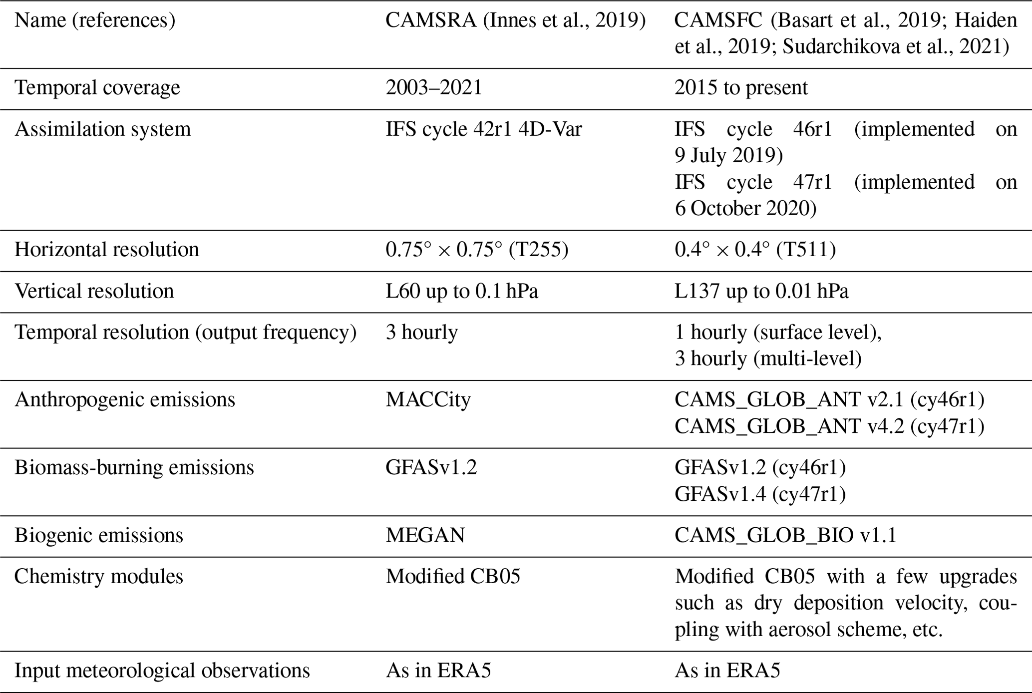
This study uses two data products, namely CAMSRA and CAMSFC, that have been produced by the ECMWF in the framework of the CAMS. These datasets focusing on surface ozone are introduced in the following subsections. An overview of the main differences and similarities between both products is given in Table 1. For more details on other aspects, the reader is referred to the references.
Table 1An overview of similarities and differences between the CAMSRA and CAMSFC datasets used in this study.
2.1.1 CAMS reanalysis
CAMS reanalysis (CAMSRA) is the latest (state-of-the-art) global CAMS reanalysis dataset of atmospheric compositions. They are produced using a four-dimensional variational (4D-Var) scheme as an assimilation technique. The chemistry module of the CAMS relies on the IFS (CB05) tropospheric chemistry mechanism with 52 species and 130 reactions (Huijnen et al., 2010; Flemming et al., 2015; Huijnen et al., 2020). Dry deposition velocities are derived from the SUMO model (Michou et al., 2004). Anthropogenic emissions are based on the MACCity inventory (Granier et al., 2011), with modified wintertime CO emissions over North America and Europe (Stein et al., 2014). Monthly mean biogenic volatile organic compound (VOC) emissions are derived offline from MEGAN (Guenther et al., 2006), using NASA's Modern-Era Retrospective Analysis for Research and Applications (MERRA) reanalyzed meteorological fields (Sindelarova et al., 2014). Daily biomass-burning emissions originating from the Global Fire Assimilation System, version 1.2 (GFASv1.2; Kaiser et al., 2012) are inferred from satellite observations of fire activities. The meteorological model consists of the given version of the Integrated Forecast System (IFS), i.e., CY42R1, with an interactive ozone and aerosol radiation scheme. Compared with the previous atmospheric chemistry CAMS reanalysis data, CAMSRA has a finer horizontal resolution of 80 km with 60 vertical model levels, with the top level at 0.1 hPa. CAMSRA covers data for the period of January 2003 to December 2021. The data are archived in 3-hourly time intervals. Hereafter, the ozone from this dataset is called O.
2.1.2 CAMS forecast
In addition to the aforementioned datasets, CAMS forecast (CAMSFC) issues (and produces) a daily global forecast of atmospheric compositions twice a day, which is initialized from analysis at 00:00 and 12:00 UTC. The forecast consists of more than 50 chemical and 7 different aerosols, providing also several meteorological parameters. Compared with CAMSRA, in CAMSFC the initial conditions of each forecast are obtained from analysis of atmospheric composition in near-real time, i.e., combining the previous forecasts with satellite observations using the 4D-VAR data assimilation technique. CAMSFC uses an atmospheric model to determine the evolution of the concentration of all species over time for the next 5 d. Apart from the required initial state, it also uses inventory-based or observation-based emission estimates as boundary conditions at the surface. Biogenic emissions originate from CAMS-GLOB-BIO v1.1, which is calculated from the MEGAN v2.1 model using ERA-Interim meteorology (Sindelarova et al., 2022). The monthly average of anthropogenic emissions is derived from the CAMS_GLOB_ANT v2.1 inventory based on a combination of EDGAR v4.3.2x and CEDS emissions (Granier et al., 2019). Biomass-burning emissions are based on GFAS. Dry depositions of trace gases are calculated online. Sulfur species, nitrate, and ammonium are coupled between chemistry and aerosol schemes. In contrast to CAMSRA, CAMSFC is available at a finer horizontal resolution of 40 km. CAMSFC is upgraded regularly, e.g., once a year, during which the model's resolution can change or new species can be added. From 9 July 2019 onwards, CAMSFC uses the assimilation system's IFS CY46R1, in which the vertical model levels have been upgraded from 60 to 137. Details of other upgrades to this system can be found in Haiden et al. (2019) and Basart et al. (2019). IFS CY47R1 was used on 6 October 2020, with some upgrades in observations, emissions, and model changes (Eskes et al., 2021; Sudarchikova et al., 2021). The temporal coverage of CAMSFC is from 2015 to the present, with temporal resolutions of 1 hourly (only for surface fields) and 3 hourly. This study uses 3-hourly forecast fields from 00:00 UTC up to 24 h. Hereafter, the ozone from this dataset is called O.
2.2 In situ measurement datasets
Surface-based measurements of ozone were extracted from the Tehran air quality control portal, which is publicly available, for 21 stations. A couple of the stations contain no data records, and the data sparsity at the stations differs from year to year. Hourly time series of surface ozone for other cities are not accessible to the public and were obtained from the Iranian Environmental Protection Organization for 54 air quality monitoring stations. We added the Geophysics station, which is located at the Geophysics Institute, University of Tehran, in Tehran. This station measures surface ozone along with several other variables such as air temperature, nitrogen oxide, wind, total ozone column, etc. Most of the air quality monitoring stations in Iran are installed in the cities, as they are aimed for the public health report. There is no information about stations' type or availability of the data at background sites. To have a common quality, the validity of the data was checked by performing a few statistical tests, such as (1) range test: verifies if the values are within the acceptable range limits (Zahumenský, 2004; Taylor and Loescher, 2013); (2) constant value test: checks the required variability among successive values (Zahumenský, 2004); and (3) discontinuity test: identifies suspicious data points before and ahead of the discontinuities (Zurbenko et al., 1996; Gerharz et al., 2011). We use the stations containing data for the year 2020, where more than 50 % of the data are available for each month. Table A1 lists the names and geographical locations of the stations, of which the first 22 are ordered based on the stations' latitudes. In Table A1, there is a number along with the stations' names, and hereafter the stations are referred to using these numbers. To include more stations in the analysis, we consider five more stations in Table A1, i.e., from 23 to 27, for which only 1 or 2 months of 2020 contain less than 50 % of data (see Fig. A1). The distribution of the stations is shown in Fig. 1, which covers three large cities (Tehran, Shiraz, and Tabriz) and six small cities (Birjand, Gilan, Hamedan, Zanjan, Markazi, and Yazd). Hereafter, the observation datasets and observed ozone time series are called OBS and O, respectively.
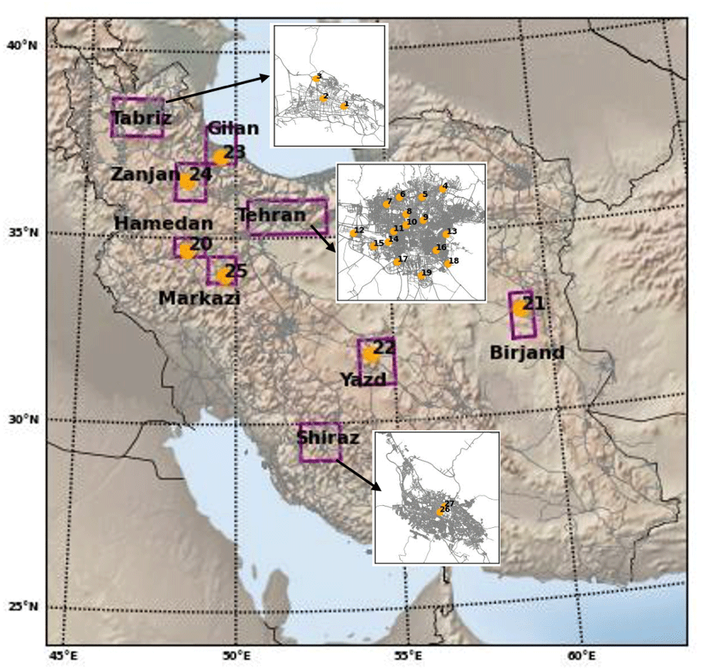
Figure 1Geographical location and distribution of the measured air quality stations used in this study. The purple-boxed areas correspond to the locations of the cities. Here the stations are represented with a number, whereas details on the name and geographical coordinates of the stations are given in Table A1. The arrows refer to the stations, which are overlaid on the city maps of Tabriz, Tehran, and Shiraz (Fars).
Both reanalysis and forecast datasets were co-located with OBS through temporal and spatial interpolations. OBS data are available in hourly resolution, in contrast to the CAMS datasets that are available in 3-hourly intervals. To match the frequency of the CAMS outputs with OBS, 3-hourly observed values are considered in such a way that at least two hourly values are available; otherwise, it renders the value as missing.
This section is divided into three sections. Section 3.1 details the theory of decompositions and the method used in this study. Section 3.2 describes the procedure for neural network modeling and the pre-processing of its input. Section 3.3 defines the metrics (indicators) that are used to assess the CAMS performance and error sources.
3.1 Spectral decomposition of the time series
The presence of various scales of motion, which are caused by several physical and chemical processes, in the time series of O3 can complicate the analysis and interpretation of data. As an example, short-term and fast fluctuations in the O3 time series are majorly attributed to chemical processes such as NO titration, whereas long-term and seasonal variations are mainly related to solar radiation, long-range transport, and stratosphere–troposphere exchange (Monks, 2000). Scale analysis is a method by which the time series can be separated into different temporal terms. Here, the time series of O3 is decomposed into three different spectral components, namely short (period less than 2 d), medium (period of 2–21 d), and long (period longer than 21 d) terms, by applying the Kolmogorov–Zurbenko (KZ) technique (Rao et al., 1997). The KZ technique is essentially a low-pass filter that consists of repeated moving averages. Its use has been demonstrated in earlier studies (Hogrefe et al., 2000; Kang et al., 2013; Seo et al., 2014). A detailed discussion of the KZ filter along with a comparison with other separation techniques can be found in Eskridge et al. (1997) and Loneck and Zurbenko (2020). The KZ technique requires two input parameters, KZ (m and k), where m is the window size for filtering and k is the number of iterations. Since the values that have been commonly used for m and k in the literature may not be applicable for 3-hourly data, we selected them based on the criteria suggested in Yang and Zurbenko (2010):
The KZ technique filters out all periods that are less than p, i.e., the number of filtered time intervals. Therefore, three components of interest in this study are estimated as follows:
where O refers to the original time series and S, M, and L indicate the short, medium, and long terms, respectively. Here, the units of O and the spectral terms are in nmol mol−1. As expected from Eq. (1), KZ(5, 5) filters all periods less than 11.2 time steps. This corresponds to 33.54 h, or 1.4 d, as the data are recorded at intervals of 3 h. The same holds for KZ(35, 5), which filters all periods less than 9.8 d. Hence, the S refers to the short-scale fluctuations, which are done in less than 1.4 d. Similarly, M refers to synoptic-scale events with timescales ranging from 1.4 to 9.8 d. The variations with timescales of more than 9.8 d are represented in the L term.
3.2 Statistical downscaling
To bridge the spatial scaling issue between coarse resolution CAMS datasets and local-scale measured data, statistical downscaling (SD) methods have been developed (Wilby and Wigley, 1997). SD refers to the use of statistical-based techniques to determine a relationship between global-scale models' outputs and observed small-scale (local) variables (Wilby et al., 2004; Wilby and Dawson, 2013). There are numerous SD methods, such as linear regression (Sachindra et al., 2013; Beecham et al., 2014), stochastic weather generators (Wilks, 1999; Kilsby et al., 2007; Semenov and Stratonovitch, 2010), and artificial neural networks (Tripathi et al., 2006; Ahmed et al., 2015; Sachindra et al., 2018; Sebbar et al., 2023), to name a few. In this study, a deep learning method known as the LSTM network was used to analyze the complex relationship between O3 and its precursors. LSTM is a modified version of a recurrent neural network designed to handle long-term (and short-term) dependencies in sequential data (Hochreiter and Schmidhuber, 1997). LSTM contains memory cells that can hold (and store) information for a long time, thus making them suitable for time series analysis. The standard LSTM consists of three gates: input, forget, and output gates for controlling the movement of information. We use Keras, a high-level neural network Python library (“Keras: the Python Deep Learning library”; Chollet et al., 2015; https://keras.io, last access: 15 May 2014) to build and train the LSTM model. This model requires a specific configuration and tuning to work effectively with the datasets. A range of control values for several hyperparameters (Table A2) were tested by multiple trial-and-error tests. The most effective hyperparameters (Table A5) were selected using the random search optimization method.
To prepare the LSTM inputs, several meteorological variables (Table A3) were obtained from the CAMSRA and CAMSFC datasets. To prevent overfitting of the model, a cross-validation LASSO regression was performed to identify the potential predictors at each station. The lagged O3 (from OBS) was also considered as one of the model inputs, since the concentration of O3 is not only affected by meteorological factors but also by the influence of the O3 levels in the past. A partial autocorrection function was utilized to estimate the correlation between observed O3 at time T and earlier time steps. For most of the stations, the autocorrelation coefficients decrease after a time lag of 24 h within a confidence interval of 95 %. So, the O at times T-1,…, and T-8, were also considered predictors at each station. Selected predictors and observed O3 were decomposed using Eqs. (2)–(4).
In order to provide the final output, i.e., downscaled O3, the LSTM architecture was trained on the decomposed datasets. The data records were divided into 65 % for the training subset and 35 % for the validation subset. The best model was chosen based on the R2 (coefficient of determination) score and mean square error (MSE). The selected model was applied to all data records to provide a downscaled output. All these procedures were applied to each station separately and are illustrated in Fig. 2.
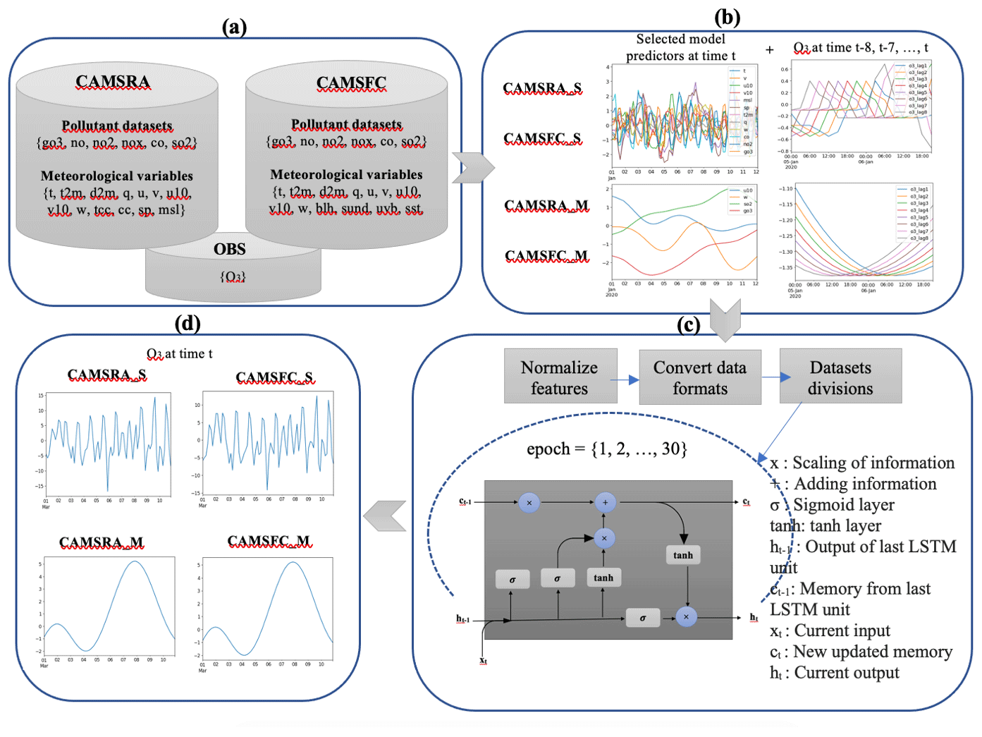
Figure 2A schematic of the downscaling processes: (a) input data retrieval, (b) decomposition and prescreening, (c) LSTM modeling, and (d) downscaled datasets.
3.3 Model evaluation
We use the mean square error (MSE) as a metric to evaluate the models' performance. The MSE is defined as the squared mean of the difference between modeled (xm) and observed (xo) variables.
This metric can be modified to include all relevant model evaluation indicators, i.e., bias, variance, and correlation, as (Murphy, 1988; Solazzo and Galmarini, 2016)
where σm and σo refer to the standard deviation of the modeled and observed data, respectively, and r is the coefficient of correlation between the observed and assimilated datasets. In Eq. (5), the first term (hereafter E1) shows the deviation between average modeled () and measured () datasets and refers to the model accuracy. The second term (hereafter E2) contains the variance error, i.e., the discrepancy in amplitude or phase between the variability in the modeled and observed values, that determines the precision of the model. Also, the third part (hereafter E3) refers to unsystematic errors related to the associativity between observed and assimilated datasets. In other words, the E2 indicates an explained error, which reveals the variance error arising from the variability in the modeled variables that are not observed in measurements. That could arise from overfitting associated with complex chemical processes in the model or imbalance among coupled components. The E3 represents an unexplained error, reflecting the lack of observed variability in the modeled data. That refers to the variabilities which are not captured by the models, even though those variabilities exist in the observations. The E3 can arise from random and non-representative errors caused by sub-scales and non-resolvable processes in the observations, or from a deficiency in the model in capturing meso-scale phenomena. Due to the spectral decomposition of the data, the S and M components have zero mean fluctuations. Hence, the E1 term in Eq. (5) is zero, and only the E2 and E3 terms are analyzed below.
To compare the distribution of error in modeled O3 before and after downscaling, the skill score (SS) is calculated as (Wilks, 2006)
Here, MSEref and MSE refer to the MSE of O (or O) and downscaled O3 (O), respectively. The value of SS varies between 0 and 1. The value is zero once there is no preference in O with respect to O (or O), i.e., the O3 variability is not explained by selected predictors. The value of SS is one when the MSE of O is zero, which means the whole O3 variability in the LSTM model is explained by the predictors, i.e., the LSTM model is perfect.
4.1 Spectral components
The time series of O3 and all meteorological variables for OBS and CAMS datasets decompose into three spectral components, short (S), medium (M), and long (L), by applying the method (KZ filter) explained in Sect. 3.1. Figure 3 shows the original time series of O, O, and O, as well as their estimated spectral components at the first station. To clearly see the signals, we only show part of the time series, here for the summer months (June, July, and August: JJA). Looking at the original 3-hourly time series (Fig. 3a), both CAMS datasets overestimate and underestimate ozone during different periods, but it is difficult to determine any clear patterns or identify specific reasons for the model bias. The S component contains frequent fast oscillations occurring every day with regular maxima and minima (see Fig. 3b). In this figure, the amplitude of the S oscillations of the O and O is different from that in OBS, indicating differences in the diurnal cycle of observed and simulated ozone mixing ratios. The M term captures variability on the timescale of synoptic systems. Some episodic events are more visible in the M component than in the S component. For instance, in Fig. 3c, the M component of the OBS represents a clear signal of an episodic event in the middle of June. This episode is not well captured in CAMSRA, whereas it is captured in CAMSFC. It seems that for most of the periods, the variations in the M component in both CAMS datasets are in good agreement with those in OBS, while the amplitudes of oscillations in CAMS do not correspond well with those in OBS. The underestimation and overestimation of the amplitude (with respect to observations) in CAMSFC is less than that in CAMSRA. Compared with the S and M terms, which oscillate around zero, the mean values of the L components are not zero (see Fig. 3d). The L represents variations in the ozone mixing ratios on seasonal, semi-seasonal, and multiannual timescales. Comparing the variations in CAMSRA and CAMSFC with OBS for L shows more similarity between CAMSFC and OBS than between CAMSRA and OBS. Both models exhibit a high bias with respect to the ozone mixing ratios. Nevertheless, the decomposition of the L component is not reliable due to the limited period (1 year) of the available data, so hereafter we only assess the S and M components.
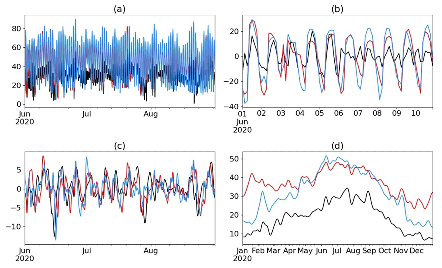
Figure 3Different spectral components: (a) original time series, (b) short (S), (c) medium (M), and (d) long (L) term of O (black), O (red), and O (blue) at station 1. The vertical axis in all panels shows the ozone mixing ratio (in nmol mol−1).
4.2 Variable selections
The time series for 16 relevant meteorological variables were extracted from CAMS products. To avoid model overfitting, we identified potential predictors of the variables. To decide on the importance of the variables, we used the LASSO-CV estimator. The relationships between predictors and O were estimated by performing a least absolute shrinkage and selection operator (LASSO) regression. The variables with the highest absolute LASSO coefficient (importance weight) are considered the most important. Figure 4 shows that the T2m is the most explanatory meteorological variable and NO, NO2, and O are the main chemical variables for CAMSRA_S at most of the stations. The variables with high feature importance (weight >0.1) were considered for use in the LSTM modeling.
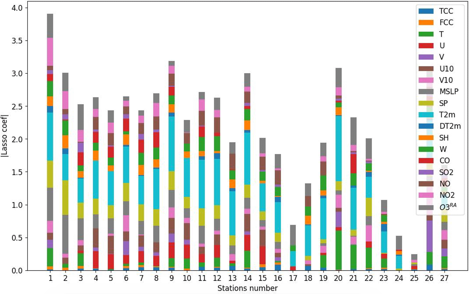
Figure 4Cross-validation LASSO regression to identify the potential predictors for ozone modeling. The higher the absolute LASSO coefficient, the more important would be the variable.
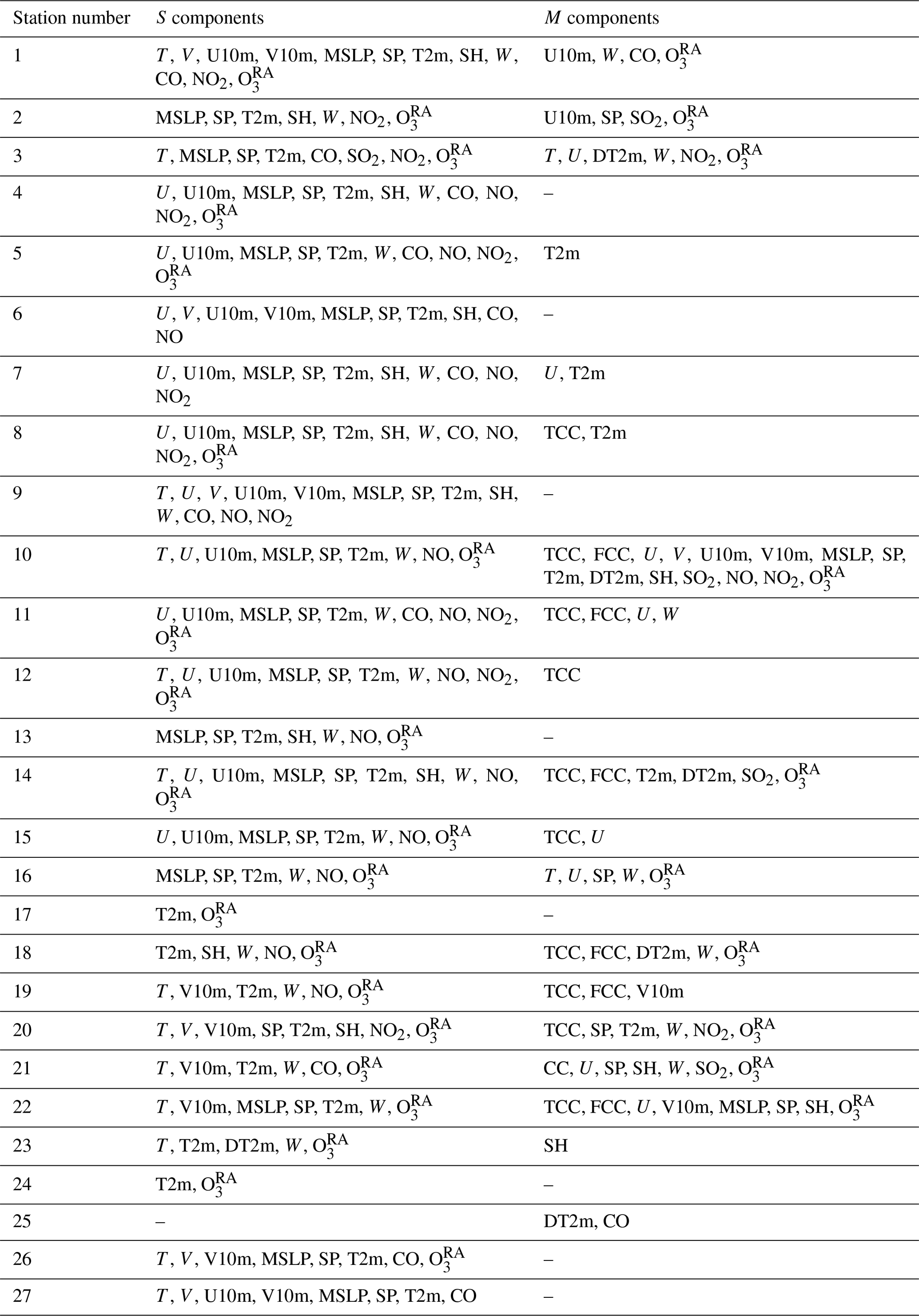
Table 2 lists selected predictors for both components of CAMSRA at each station. At station 1, 12 variables, namely T, V, U10m, V10m, MSLP, SP, T2m, SH, W, CO, NO2, and O, are identified as the potential predictors of the S component, while four variables, i.e., U10m, W, SO2, and O, are selected for the M term. Some of the selected predictors are common between the S and M components. A few meteorological variables, such as T2m, SP, MSLP, W, and U10m (or V10m), appear for the S component at most of the stations. These variables reflect the information about temperature, pressure, and vertical velocity. Temperature is one of the key meteorological factors influencing the S term variability in O3 through its effect on biogenic emissions, photochemical kinetics reaction rate, and anthropogenic emissions. Stable anticyclones and sunny conditions promote O3 formation and accumulation. Zonal and meridional winds at 10 m are important for the dispersion of ozone precursors at local scales. For most of the stations, the S term is affected by pollutant species such as O, NO, and NO2, of which NO and NO2 are recognized as potential drivers of O3 levels. Selection of total cloud cover (TCC) and fraction of cloud cover (FCC) for the M component at most stations indicates that cloud covers are mostly associated with synoptic systems (e.g., occurrence of high pressure systems associated with clear-sky conditions) and O3 variability on this scale. The M component at a few stations, e.g., 4, 6, 9, and 13, shows weak associations with the parameters, so no variables are selected for them. This situation often happens for the M component and suggests the role of other factors (not included in the predictors). There are a few stations where O (O) is not selected as an important variable, which is related to the small (weak) associations between O (O) and O. For instance, SH is selected as the main factor effecting the M term at station 23, i.e., Rasht. This station is located between the mountains (Alborz) and coast (Caspian Sea), with a local rainy environment and a humid subtropical climate. That is similar to the western Mediterranean regions, where a lack of strong synoptic advection, combined with the orographic characteristics and the land–sea breezes, favors episodes of high ozone levels over this region (Millaìn et al., 2000; Velchev et al., 2011; Wentworth et al., 2015). Similar to CAMSRA, for CAMSFC the number of selected parameters for the S is larger than that for the M (see Table A4). In CAMSFC, boundary layer height (BLH) and V10m (or U10m) appear as dominant meteorological drivers affecting the S component. Stable boundary layer height causes the accumulation of ozone and its precursors during night or under light (weak) winds conditions. Moreover, ozone in residual layers can be transported over long distances with prevailing winds. In the morning, trapped ozone can be entrained downward into the mixed layer (Stull, 1988; Zhang and Rao, 1999). The M term is mostly associated with O.
Table 2The most important explanatory variables of CAMSRA at each station.
4.3 LSTM model and validation
The LSTM model was trained and validated with the datasets, as explained in Sect. 3.2. We tuned hyperparameters, which allow the learning algorithm to run until the error from the model, i.e., the loss function, has been sufficiently minimized. As there are no given values to set these numbers, the optimum values were obtained by multiple trial-and-error tests (see Table A5). The best model was selected based on the MSE and R2 (coefficient of determination) score, which indicates the amount of explained variance by the LSTM model. Figure 5 shows the R2 of the selected model for all data series at each station. For most of the datasets, the R2 is larger than 0.5, indicating that more than 50 % of the O3 variance is explained by the LSTM. The R2 for the M component is larger than that for the S term, despite the smaller number of predictors for the M. This might reflect that the M component is easier to be modeled due to less complexity. In this figure, the R2 of the M is around 0.9 for all stations, whereas it varies for the S term. The R2 value of the S at the stations over the city of Tehran is within the same range of 0.7–0.8. Both CAMSRA and CAMSFC show the R2 to be less than 0.5 for the S term at a few stations, namely 22 (Yazd), 24 (Zanjan), and 25 (Markazi). A possible reason for that could be the peculiar characteristics of short-term ozone variability at these sites or their geographical locations. Model-to-model differences in R2 are more pronounced in the S, which is likely due to the different emission inventories used in the models.
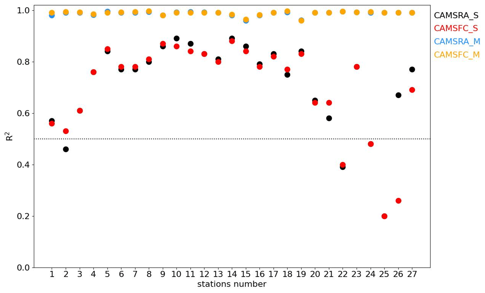
Figure 5The R2 of the LSTM model for both S and M components of O3. CAMSRA_S and CAMSFC_S refer to the S components of CAMSRA and CAMSFC, respectively. Likewise, CAMSRA_M and CAMSFC_M refer to the M components of CAMSRA and CAMSFC, respectively.
Figure 6 shows the box plots of MSE and different terms of MSE, i.e., E2 and E3, for both components of O. For the sake of simplicity, descriptions of the results are mostly based on the mean values. Nevertheless, the values of the indicators at each station are shown as a scatter point next to the box plots. From Fig. 6a, it turns out that the mean MSE (shown with red squares) of O3 for the S component is larger than that for the M component for both models. That could arise from the uncertainties in O3 precursor emissions affecting modeled local photochemistry and likely S variability. The largest value of the MSE is associated with the O of the stations located in the city of Tehran. That can be associated with the uncertainties in CAMS emission inventories, which may have a larger impact in cities with high anthropogenic emission sources. The stations in the northern part of the city (e.g., stations 4–9) show a larger MSE than the stations in the southern part (e.g., stations 10, 11, 14–17, and 19). That can be associated with the deficiency in the emission inventories in capturing the local emission changes within urban areas. The large value of MSE is also found for the S term at the stations located in Shiraz and Tabriz, which are known as big and highly populated cities with numerous local anthropogenic emission sources (thermal power plants, oil refinery, cars, etc.). Station 2 in Tabriz shows less MSE than stations 1 and 3, which are located in the industrialized part of the city. That can be associated with the uncertainties in the spatial variations in the emission inventories used in CAMS. Although the CAMS anthropogenic emission inventories account for emissions from different sectors, such as transportation, residential and energy sectors, as well as biogenic fluxes, they have a temporal and spatial allocation with a monthly spatial grid resolution of 0.1° × 0.1°. Low values of the MSE for CAMSRA_S and CAMSFC_S are attributed to stations 22 (Yazd), 20 (Hamedan), and 24 (Zanjan). Similar to R2, the lowest MSE belongs to the Yazd station, which contains fewer local emission sources than other cities such as Tehran, Tabriz, and Shiraz.
Figure 6b shows the explained error (E2) in CAMSRA and CAMSFC for both components. E2 is a model-related error, and a possible source for this can be a misrepresentation of short- and meso-scale phenomena in models. The small values of E2 reflect the low contributions of E2 to the MSE and the noticeable improvement in the O (via downscaling procedures). The major portions of the MSE are associated with the unexplained errors (E3) for both components (see Fig. 6c). The E3 for the S component is larger than that for M, as expected from the variance in these components. The S variability is associated with the effect of daytime photochemical production and downward transport of O3 rich from upper levels, combined with O3 loss by depositions (in the surface layer). A large value of E3 for the S component can arise from the CAMS' deficiency in resolving the meso-scale phenomena such as local winds, NO titration, deposition rates, and their influences on O3 variability. Assessing the element of E3 (see the third term of Eq. 5) shows that large variances in observations (σo) or small correlations (r) cause the large E3 and consequently the large MSE. Figure A2a shows the correlation between the models and observation datasets for both components. This figure shows that M contains a larger correlation (r>0.9) than S in both models. A high value of correlation between two terms can be attributed to the larger covariance of two terms or less variance in each term. Figure A2b shows the covariance between models and observations. As can be seen in this figure, the mean value of covariance for the S components is larger than for the M components. So, the smaller correlation of the S in comparison with that of the M is attributed to the larger variance in S (Fig. A2c). In other words, the better model performance (i.e., smaller E3 and MSE) for the M is not associated with the larger covariance of the M component. That is attributed to less variance in M than in S (see Figs. 3 and A2c).
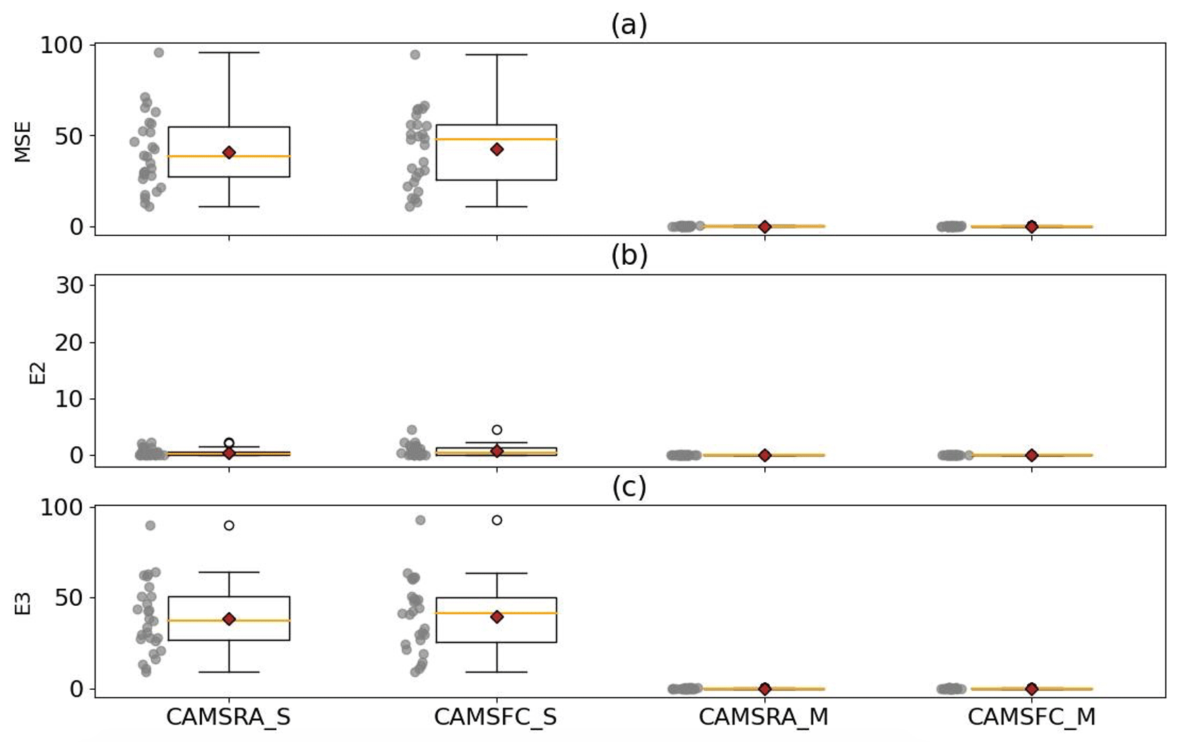
Figure 6The (a) MSE, (b) E2, and (c) E3 of the downscaled O and O with LSTM for both S and M components. CAMSRA_S and CAMSFC_S refer to the S components of CAMSRA and CAMSFC, respectively. Likewise, CAMSRA_M and CAMSFC_M refer to the M components of CAMSRA and CAMSFC, respectively.
In order to examine the effect of the CAMS products and lagged O3 (from actual observations) on the LSTM model, we exclude the measured lagged ozone from the predictors of the LSTM model (hereafter LSTMno_lag). The R2 of the LSTMno_lag is shown in Fig. A3. Overall, the R2 of the LSTMno_lag is less than that of the LSTM. This suggests that the LSTMno_lag may carry the risk of not including all important predictors (e.g., lagged ozone) in the model. This feature is more noticeable in the M term than the S term, i.e., the R2 of the S component is less affected by removing the lagged O3. That reflects the CAMS products, which explain more of the S variance than that of the M term. In other words, most of the variance in the M term in the LSTM is explained by the lagged O3 (not by the CAMS products). That could be a reason for the better performance (less MSE) of the M than the S. Figure A4a shows the MSE of the LSTMno_lag. In this figure, the MSE of the datasets increases by 2 times with respect to that of the LSTM. The higher values of the MSE in the LSTMno_lag are attributed to the removal of the observed lagged O3 from the model. Although the R2 of the LSTMno_lag for the S is larger than that for the M term, the MSE of the S is higher than that of the M term. This is similar to the MSE of the LSTM, which is related to the higher variance in S than M. Similar to the LSTM, in LSTMno_lag, the low values of MSE are seen for the S component of O3 at stations 22 (Yazd), 20 (Hamedan), and 24 (Zanjan).
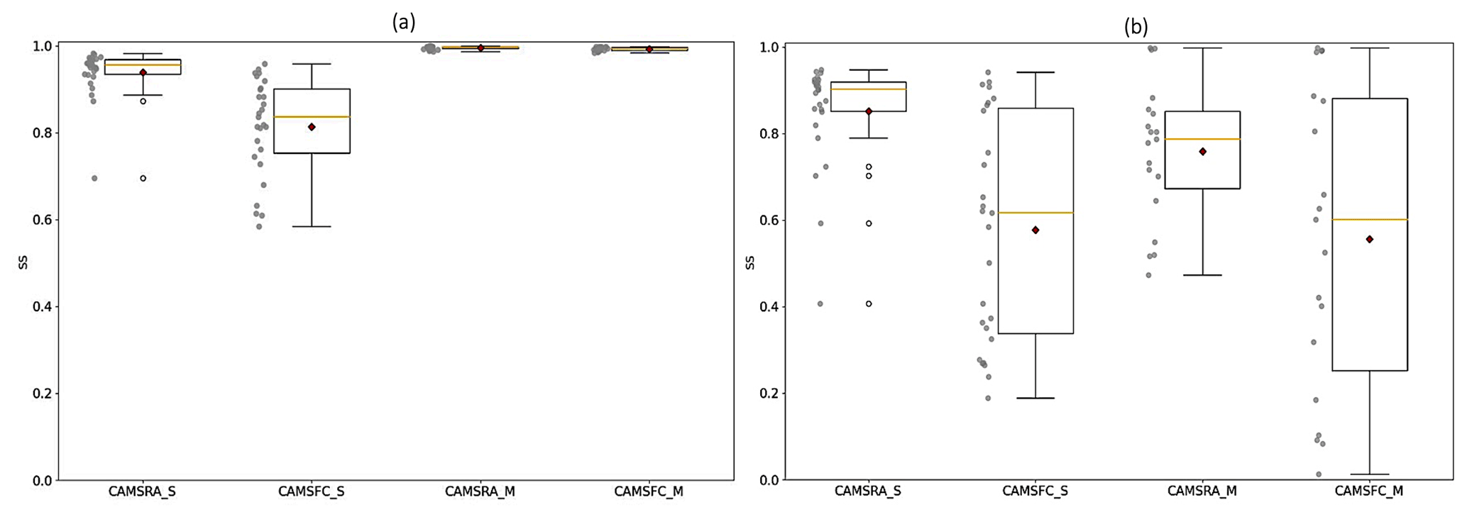
The skill scores (SS) of the downscaled models O with respect to the O and O for all datasets are shown in Fig. 7. In Fig. 7a, the mean value of the SS for three datasets, namely CAMSRA_S, CAMSRA_M, and CAMSFC_M, is larger than 0.9. This reflects that the downscaling procedure (LSTM) improves the accuracy of the results in the three mentioned datasets. The lower value of the SS for CAMSFC_S can be attributed to the higher skill of the reference dataset, i.e., O, or less accuracy of the LSTM model. The SS of the LSTMno_lag for CAMSRA_S shows the same high accuracy as that in the LSTM, whereas for other datasets the mean SS declines to less than 0.8 (see Fig. 7b). There is a large difference between the SS of the LSTM and LSTMno_lag for the M component, which shows the importance of the lagged O3 for modeling of the M term. Larger values of SS for CAMSRA than that for CAMSFC reflect a better performance of O over Iran. That is also shown in Fig. A7a, in which the MSE of CAMSFC_S is less than that of CAMSRA_S.
Analysis of the spectral components in this study reveals that the O3 variability in both CAMS products possesses a nearly similar shape (although in different phases and amplitudes) to those in OBS. Although both datasets share many of the same parameters, there are several differences that distinguish O from O. O is produced by a model with finer horizontal and vertical resolutions. Different anthropogenic and biogenic emissions have been used in both models (see Table 1). CAMS-GLOB-ANT (used in CAMSFC) provides up-to-date emissions of air pollutants and greenhouse gases at the spatial and temporal resolution required by the model (0.1° × 0.1°). CAMSRA uses MACCity emission inventory with a resolution of 0.5° × 0.5°. Figure A6 shows a comparison of CAMS-GLOB-ANT and MACCity for a couple of ozone precursors, i.e., NOx and CO. Compared with CAMS-GLOB-ANT, MACCity provides higher NOx and CO emissions. CAMS-GLOB-ANT shows more details of the emissions' variability due to the finer spatial resolution. The area with the highest emissions in both inventories is located over Tehran.
The results of the models' performances show a larger MSE for the S than for the M in both CAMS. That arises from the larger variance in the S in comparison with the M (Hogrefe et al., 2000, 2014; Kaffashzadeh, 2018; Kaffashzadeh and Aliakbari Bidokhti, 2022). The results of the error apportionment show the negligible contribution of the E2 to the MSE. The E2 arises from the limited spatial resolutions of the CAMS in capturing short- and meso-scale phenomena that are attenuated (alleviated) by the SD procedures. The MSE has mostly arisen from the E3, which emphasizes the lack of observed variability in the CAMS data. The E3 assessment shows less variability for both components of O than in O. That could arise from random errors inherent in the OBS data due to sub-scale or non-resolvable processes in an observational network. The variability in the measured data might be generated from the non-representatives errors due to random effects caused by turbulence or sub-scale perturbations (Gandin, 1988; Steinacker et al., 2011). It is not straightforward to distinguish and exclude these errors in the measured data because of their chaotic and unsystematic behavior. Adding the lagged O3 to the predictors of the downscaled model halves the E3 (and MSE). Less MSE in the M in comparison with that in the S is attributed to not only less variance in the M than in the S but also the larger contribution of the lagged O3 in the M than in the S (as shown in Sect. 4). The S component shows large associations with meteorological variables such as T2m, BLH, U10m, and V10m, as well as pollutant species such as CO, NO, and NO2. That is due to short-term O3 fluctuations associated with processes such as vertical mixing, local NO titration, deposition, wind speed, solar flux, etc.
The S component shows the large value of MSE for the stations located in Tehran, Shiraz, and Tabriz, which are known as the most populated cities (and thus large local emission sources) in Iran. The largest MSE belongs to O3 at the stations over Tehran (see Fig. A4). That can be partly attributed to the complex topography and local (meso)-scale flow (e.g., slope, mountain, and valley flow) over the city. The pollutant concentrations are highly affected by these factors, which are hardly captured by the global chemistry models (Fiore et al., 2003). The MSE of O3 over Tehran in the warm season is much higher than that in the cold season (see Fig. A5). That could arise from the uncertainty in O3 precursors in CAMS, as they are not adjusted by data assimilation systems. CAMS-GLOB-BIO (used in CAMSFC; see Table 1) provides a monthly average of the global biogenic emissions, which are calculated using the MEGAN (used in CAMSRA; see Table 1), driven by ERA-Interim meteorological fields. In summer, rising temperatures speed up the rate of many reactions and enhance biogenic VOC emissions (Sillman and Samson, 1995). The city of Tehran suffers from high levels of emitted NOx from several sources, such as road traffic, industrial activities, the energy conversion sector, etc. (Hosseini and Shahbazi, 2016; Yousefian et al., 2020). The latest Tehran emission inventory indicates that the annual emissions of VOC and NOx are approximately 91 000 and 103 000 t, respectively (Shahbazi et al., 2022). The contributions of vehicles to VOC and NOx emissions are estimated to be 79 % and 35.2 %, respectively, and increase to 79.5 % and 37.2 %, respectively, in summer. In addition to the aforementioned factors, what distinguishes Tehran from other cities is the difference between daytime and nighttime populations. During the day, traffic in Tehran reaches its highest level due to the arrival of private vehicles as well as passenger and cargo transportation vehicles from surrounding areas and cities. This issue has a significant impact on the city's traffic and the vehicle traffic on intercity routes leading to Tehran. The impact of these (meso-scale) factors cannot be captured in a global emission inventory with a limited resolution. That induces large model uncertainties, in particular for the S variability, which has large associations with pollutant species. Besides, for some periods the emissions are not available and so prescribed, which means they are either kept fixed since the last year of availability or extrapolated (projected) with a climatological trend. MACCity emission inventory has not been updated since 2010, and recent years are only based on projections of past trends. CAMS-GLOB-ANT provides the monthly average of the global emissions of 36 compounds over the period 2000–2019. The MSE distribution over Tehran is uneven: the northern part of the city shows a larger MSE than the southern part. That can be attributed to the uncertainty in the simulated CO species, as it is selected as a predictor at the stations located in the northern part. The CO concentration increases, moving from the south to the north of Tehran (Sharipour and Aliakbari Bidokhti, 2014).
Stratospheric ozone can affect surface ozone levels indirectly through vertical downward transport of ozone from the lower stratosphere and/or the upper troposphere on larger timescales (Zanis et al., 2014; Akritidis et al., 2016) or directly through intense stratospheric intrusions (rarer) (Akritidis et al., 2010; Chen et al., 2022). Over Tehran, a major portion of O3 during spring is transferred from the stratosphere (Aliakbari Bidokhti and Shariepour, 2007). A study by Shariepour and Aliakbari Bidokhti (2013) showed that several mid-latitude low pressure weather systems accompanied by tropopause folding affect northern Iran (Caspian Sea) and can cause downward transport of stratospheric ozone-rich air towards the surface. During summer, the occurrence of tropopause folding and its intensity over the eastern Mediterranean and the Middle East regions are majorly controlled by the Asian monsoon. Since the zone of upper level baroclinicity and fold occurrences spreads northwestward over this region, it first reaches Iran in July (Tyrlis et al., 2014). The large MSE of O for the cities of Shiraz and Tabriz is mostly associated with the geographical locations of the cities. Tabriz is the largest economic (industrialized) hub and metropolitan area in northwestern Iran, which is often affected by cyclonic activities (Asakereh and Khojasteh, 2021) and summer circulations over the eastern Mediterranean region (Tyrlis et al., 2013). Although CAMSRA captures the long-range transport processes and atmospheric background in the troposphere, it shows a lower skill over the Mediterranean, in particular the eastern part, compared with other regions (Errera et al., 2021). Shiraz, the capital of Fars Province, is the largest city in southwestern Iran, with more than 1.2 million inhabitants. This city has high levels of air pollutants due to population growth, urbanization, and traffic-related emissions. The city is located in a valley between two mountain ranges with east–west orientations. The model representation of the terrain is considered to be a key factor for achieving a good representation of the wind flow in complex terrain (Mughal et al., 2017). The low MSE values in the cities of Yazd, Hamedan, and Zanjan are associated with the station locations, which are less populated and affected by the emission sources.
To assess the sensitivity and robustness of the results to SD methods, the data are downscaled using another SD method, namely the multiple linear regression (MLR) model. In this model, the predictors and predictand were the same as in the LSTM model. Figure A7b shows the MSE of O with the MLR model. In similarity with the LSTM model (similar to the results in Sect. 4), the MSE for the S is larger than the M components downscaled with the MLR model, although the mean value of the MSE of the downscaled data with the MLR is slightly larger than that of the LSTM. That could arise from the larger correlation (and covariance) between downscaled datasets and OBS in the LSTM model. Similar to the LSTM, the SS of the MLR is high for all downscaled datasets; the SS for the CAMSFC_S datasets is less than that for other datasets (see Fig. A8a). Two experiments were designed to assess the sensitivity of the model to less obvious predictors. In the first experiment, i.e., MLRno_lag (expr1), the model was trained only using O and O. In the second experiment, i.e., MLRno_lag (expr2), the model was trained using the most influential meteorological variables (see Table A6). For the sake of simplicity (and being less expensive), both experiments were performed using the MLRno_lag model. Table A7 lists the results of these experiments for station 22 (Yazd). As can be seen, the MSEs of MLRno_lag (expr1) and MLRno_lag (expr2) are larger than that of MLRno_lag. This shows that part of the O3 variability is explained by meteorology and partly by the chemistry (O or O). Separating these two factors causes a decline in r (see Fig. A9).
In this paper, the variability in O3 in two datasets, namely CAMSRA and CAMSFC, was assessed against observations at 27 urban stations distributed over Iran. Our observation datasets contain time series from various cities in Iran, e.g., highly polluted cities vs. small cities. This helps identify where the models capture reality and where they need more improvement. To cope with the limited spatial resolutions of CAMS, the data were downscaled using an LSTM neural network. The potential predictors (inputs) for the LSTM were identified from chemical and meteorological variables at each station. We decomposed all time series into three spectral components, i.e., short (S), medium (M), and long (L) terms. The S term consists of intraday and diurnal variations, the M term includes synoptic multiday fluctuations, and the other motions, i.e., seasonal, semi-seasonal, and trend, are carried in the L term. We only assessed the S and M terms due to the availability of 1-year data, i.e., 2020; the L component is primarily used to check the biases between model data and observations but should not be considered reliable with respect to trend analysis, etc. Since the S and M components have zero-mean fluctuations, the bias term (the distance between the time average of model data and observations) is zero, and the main focus of this study was to analyze the variability terms, e.g., variance and covariance. The results presented in this study reveal several key points:
Various variables were identified as potential predictors of ozone. The S term shows high associations with temperature, 10 m wind components, and NOx, while the M component shows higher associations with cloud cover and simulated ozone. In CAMSFC, boundary layer height appears to be the dominant meteorological driver of the S component. The R2 of the LSTM model for the M component is larger than that for the S term, despite a smaller number of predictors for M than for S. This might reflect that the M term is easier to model.
The SS of the downscaled CAMSFC_S is lower than that of other datasets. This can be attributed to the higher skill of the reference dataset, i.e., O. The SS of the LSTMno_lag for CAMSRA_S shows the same high accuracy as LSTM, whereas for other datasets, the mean SS declines to 0.5. That shows the importance of the observed (lagged) O3 as a predictor in the LSTM. The robustness of the results was also confirmed using additional downscaling procedures, i.e., MLR.
Both datasets, i.e., CAMSRA and CAMSFC, show less MSE for the M component than for the S term. That is mainly attributed to the low variance in M and is not related to the large covariance of this component. The MSE was mainly associated with unexplained model errors (E3), which could be caused by the CAMS deficiency in resolving the meso-scale phenomena such as local winds, NO titration, deposition rates, and their impacts on O3 variability. In addition, uncertainties in emission inventories might affect this error. Including a proxy of stratospheric ozone contribution to surface ozone (stratospheric ozone tracer) may be beneficial in explaining short-term ozone variability, thus reducing the error (a recommendation for future work).
In both datasets, the highest MSE appears for O at stations in the cities with high emissions, in particular over Tehran in the warm season. That majorly arises from the uncertainty in O3 precursors, e.g., NOx, in CAMS. This can be considered a starting point for improving the results of surface ozone, in particular at urban sites.
To date, most of the studies of ozone and other pollutants in Iran rely on reanalysis products, without using decompositions or downscaling procedures. Our findings show that the CAMSRA and CAMSFC datasets have some deficiencies in simulating ozone, in particular over the cities with high emissions of ozone precursors. Downscaling improves these products and makes them suitable for the study of ozone in major metropolitan areas. The method used in this study is not only applicable for the evaluation of the global models but also for prediction purposes.
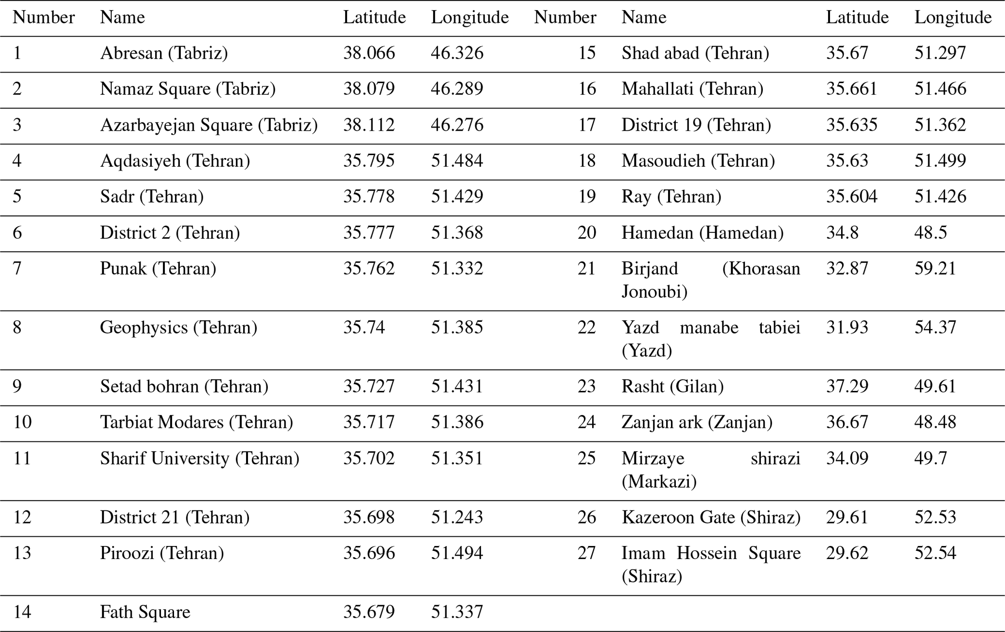
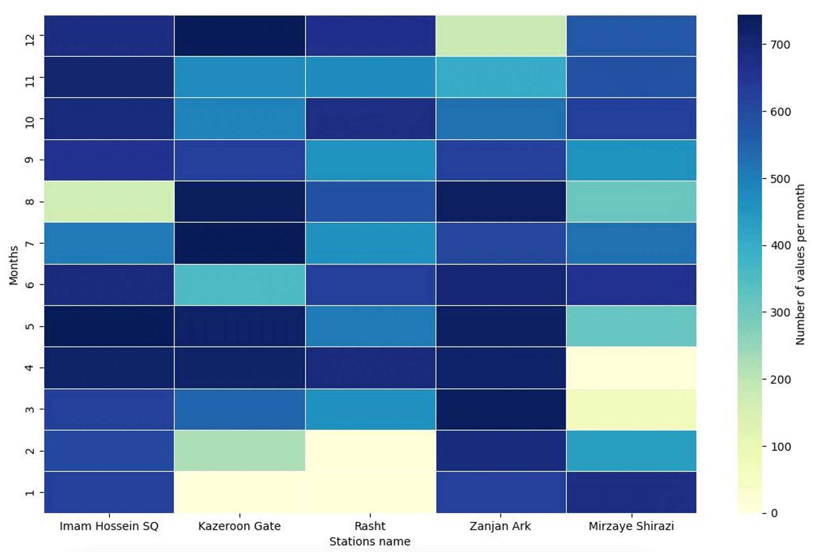
Figure A1Data coverage (per month) of the hourly surface-based measured ozone at five air quality monitoring stations.
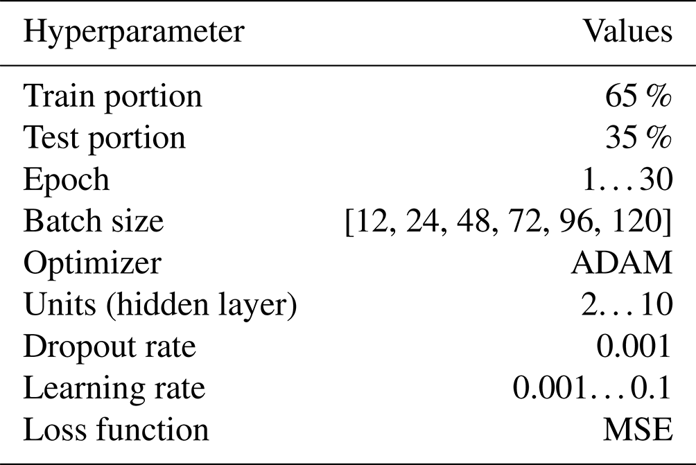
Table A3A list of the meteorological variables that were extracted from CAMS data products. ⊕ and ⊖ represent available and unavailable variables, respectively.
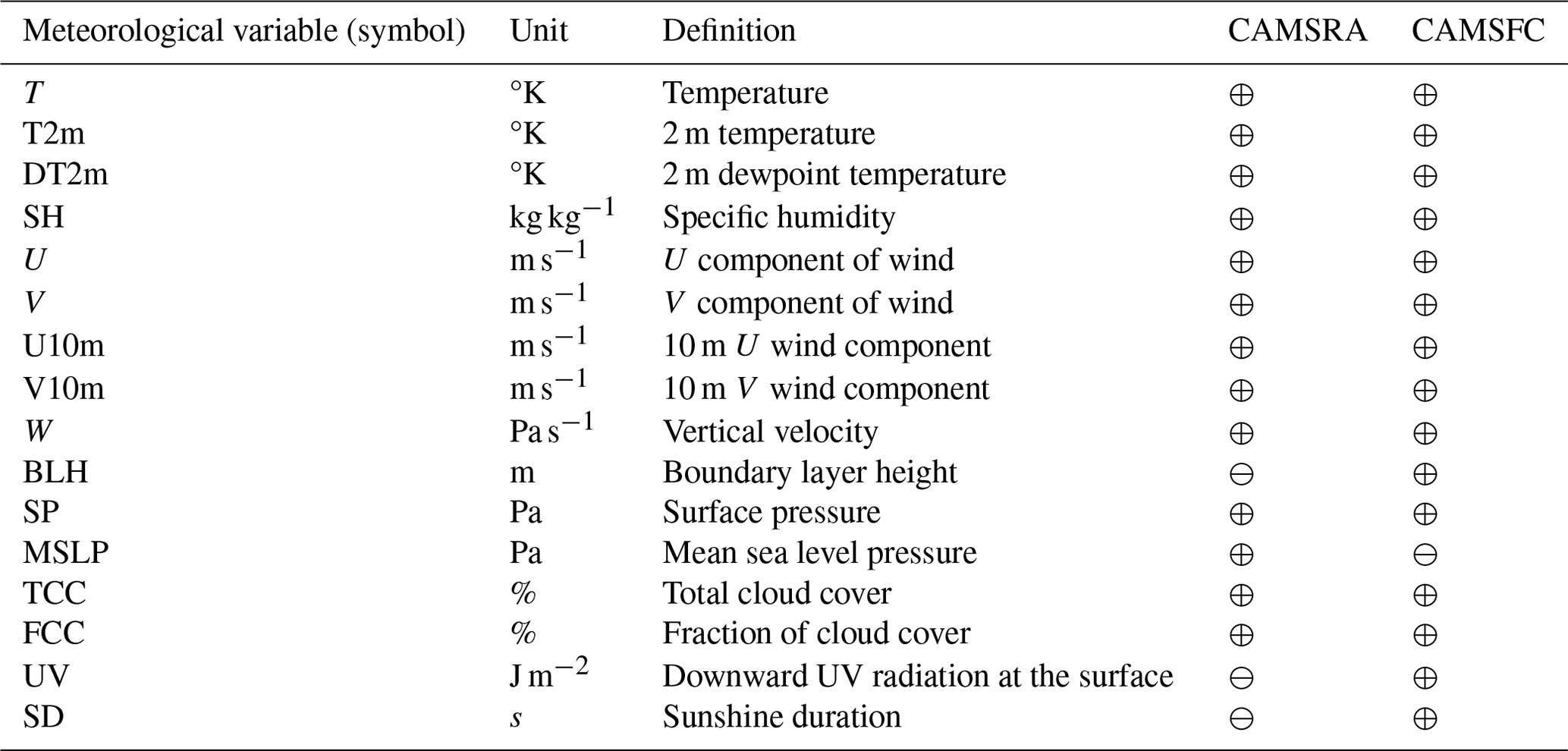
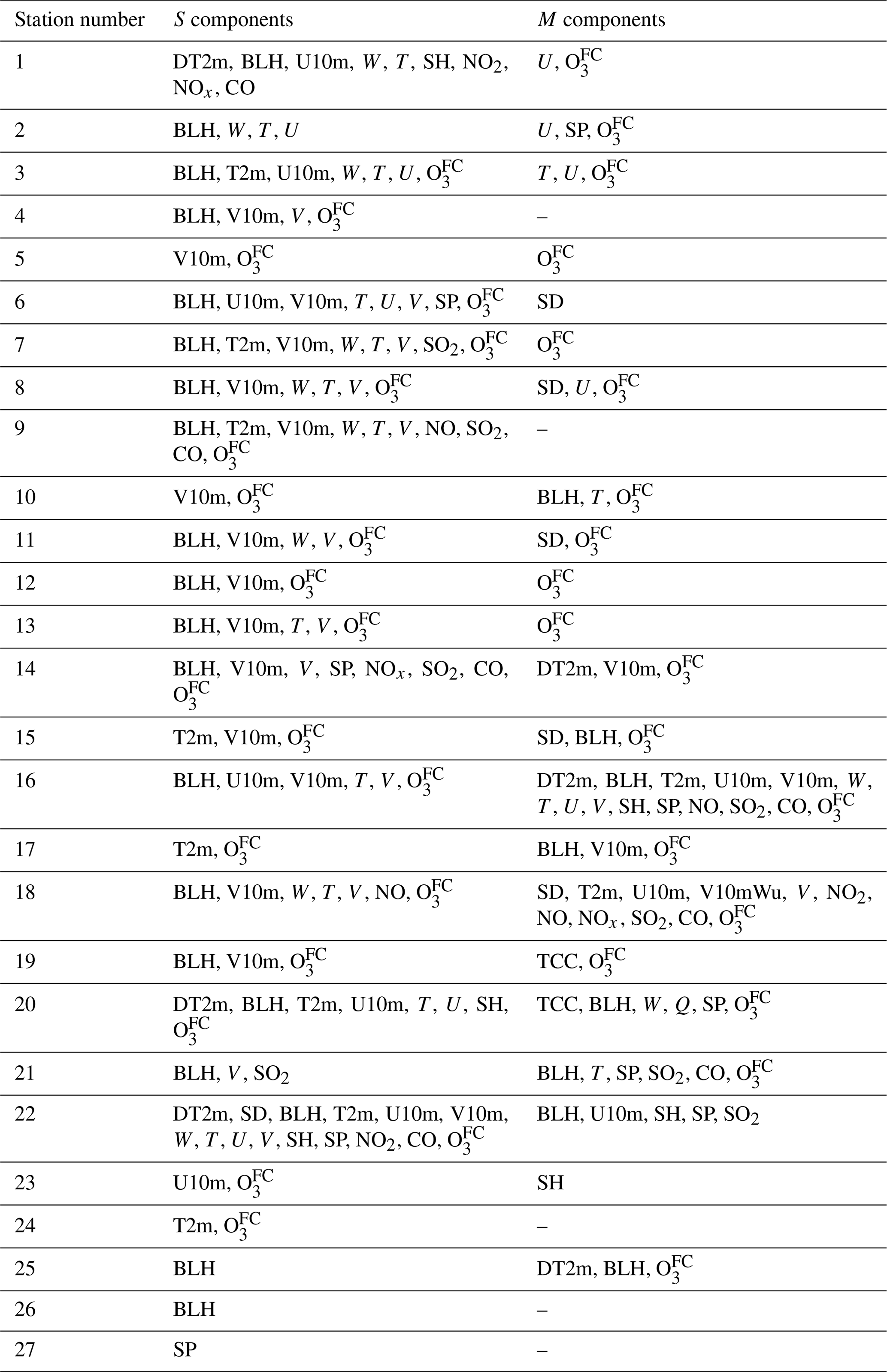
Table A5The optimum units, dropout, learning rate, and batch size for implementing the LSTM model. T: true; F: false.
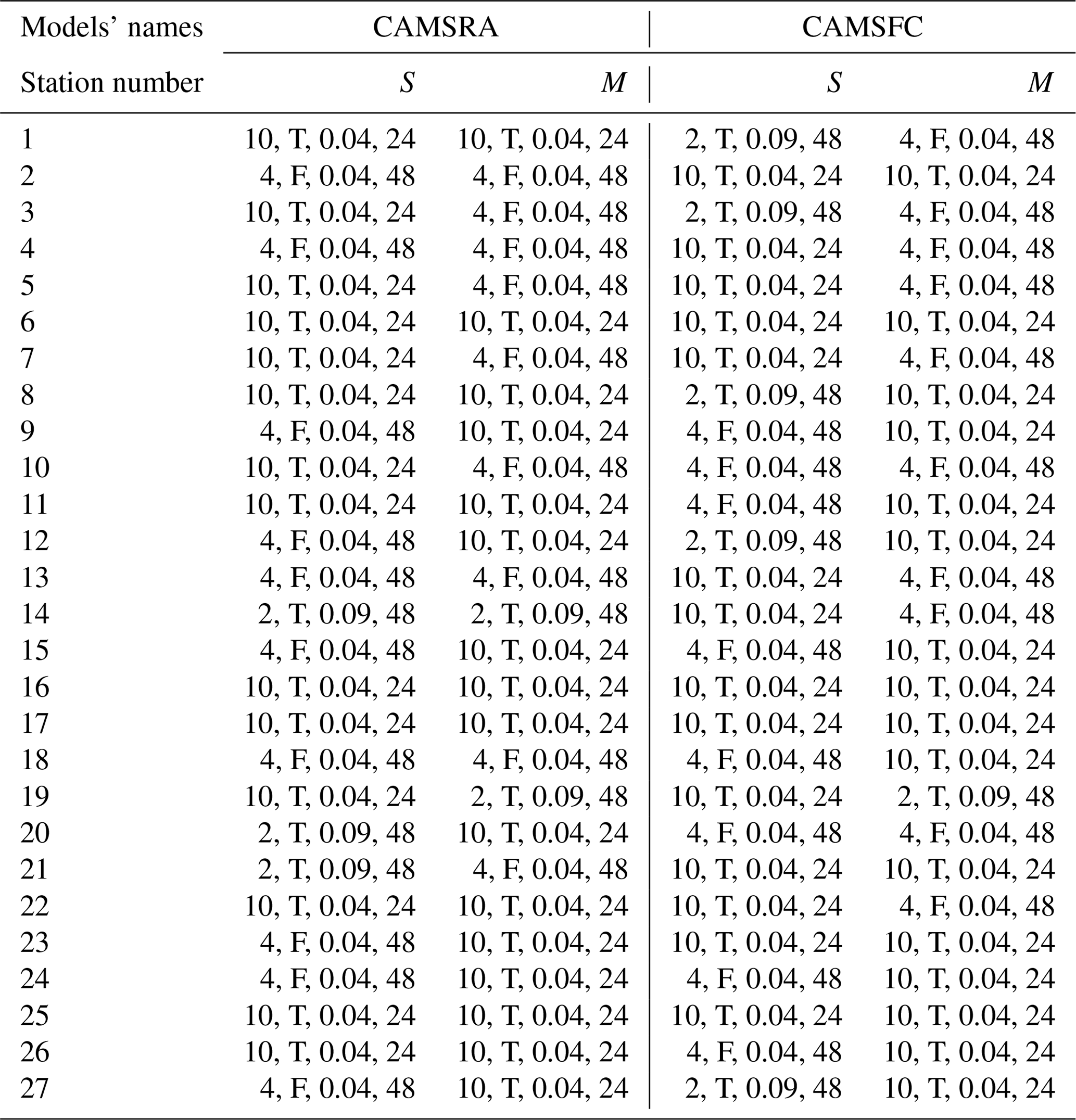
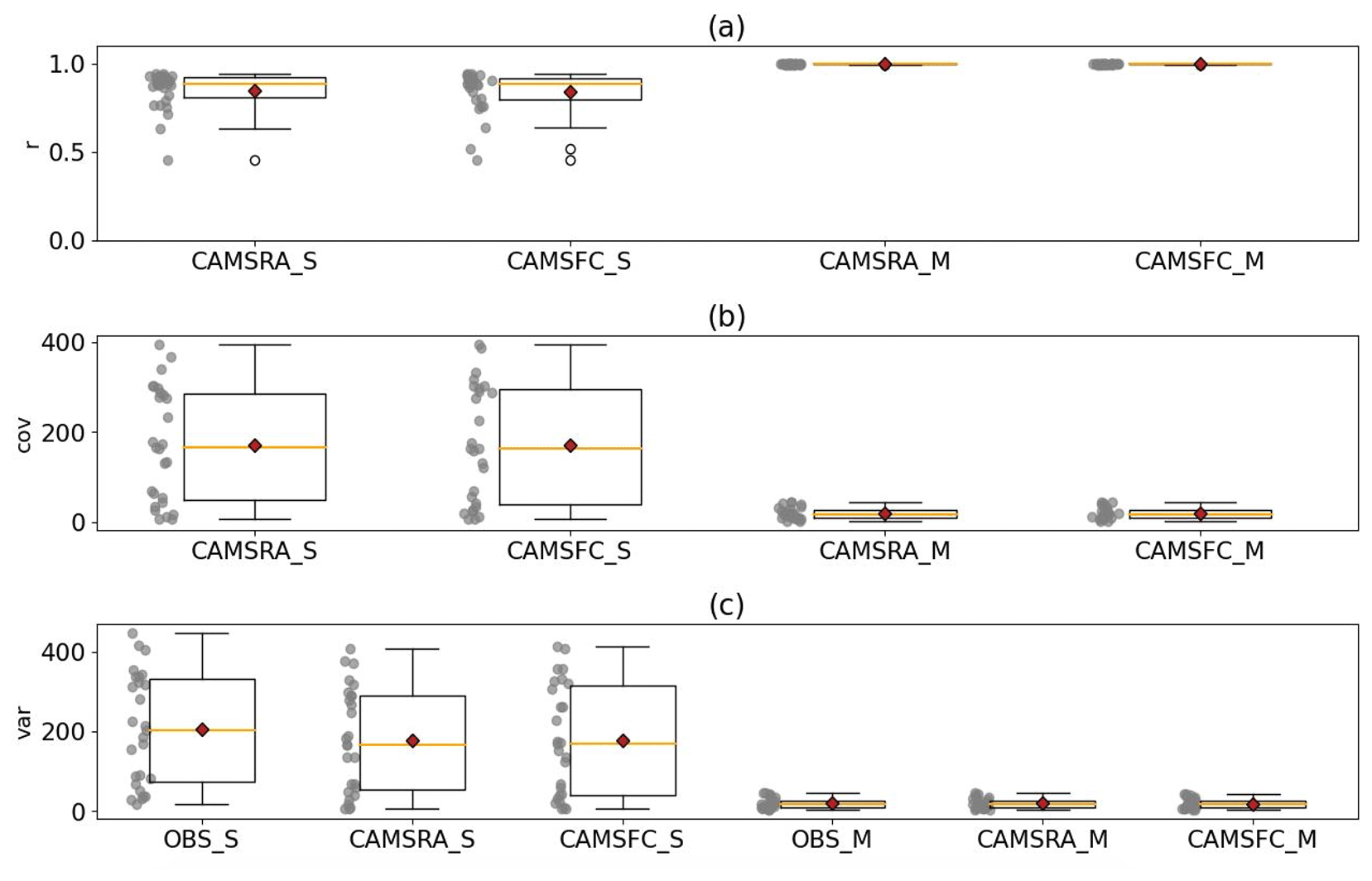
Figure A2The (a) correlation (r), (b) covariance (cov), and (c) variance (var) of the O with LSTM.
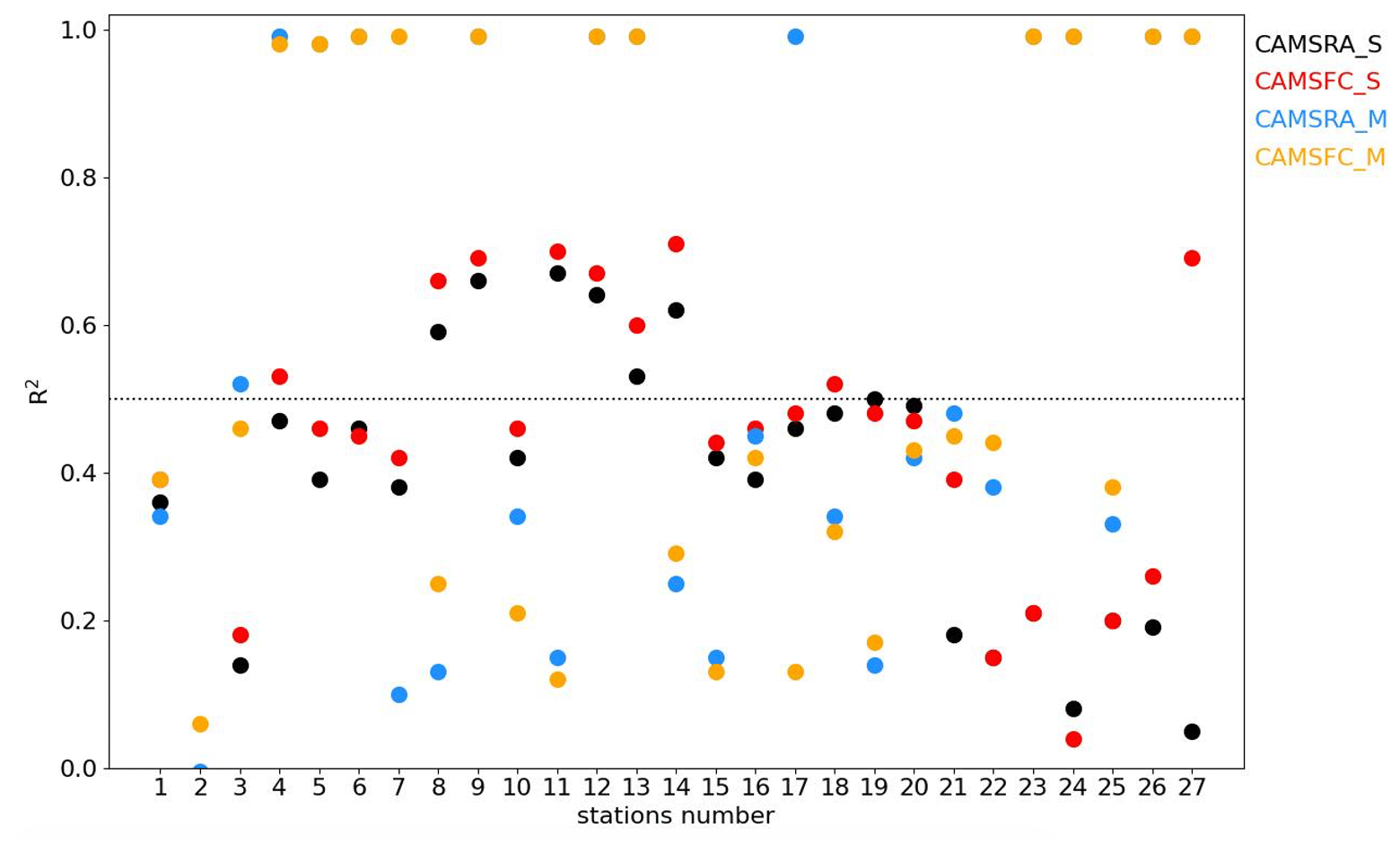
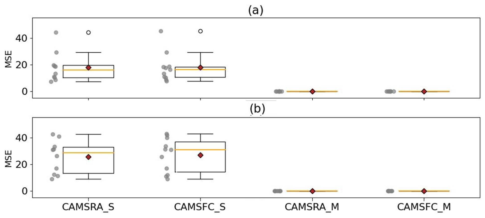
Figure A4The MSE of the O at the stations, excluding the stations over Tehran city, for (a) the cold (months 1–3 and 10–12) and (b) the warm (months 4–9) seasons.
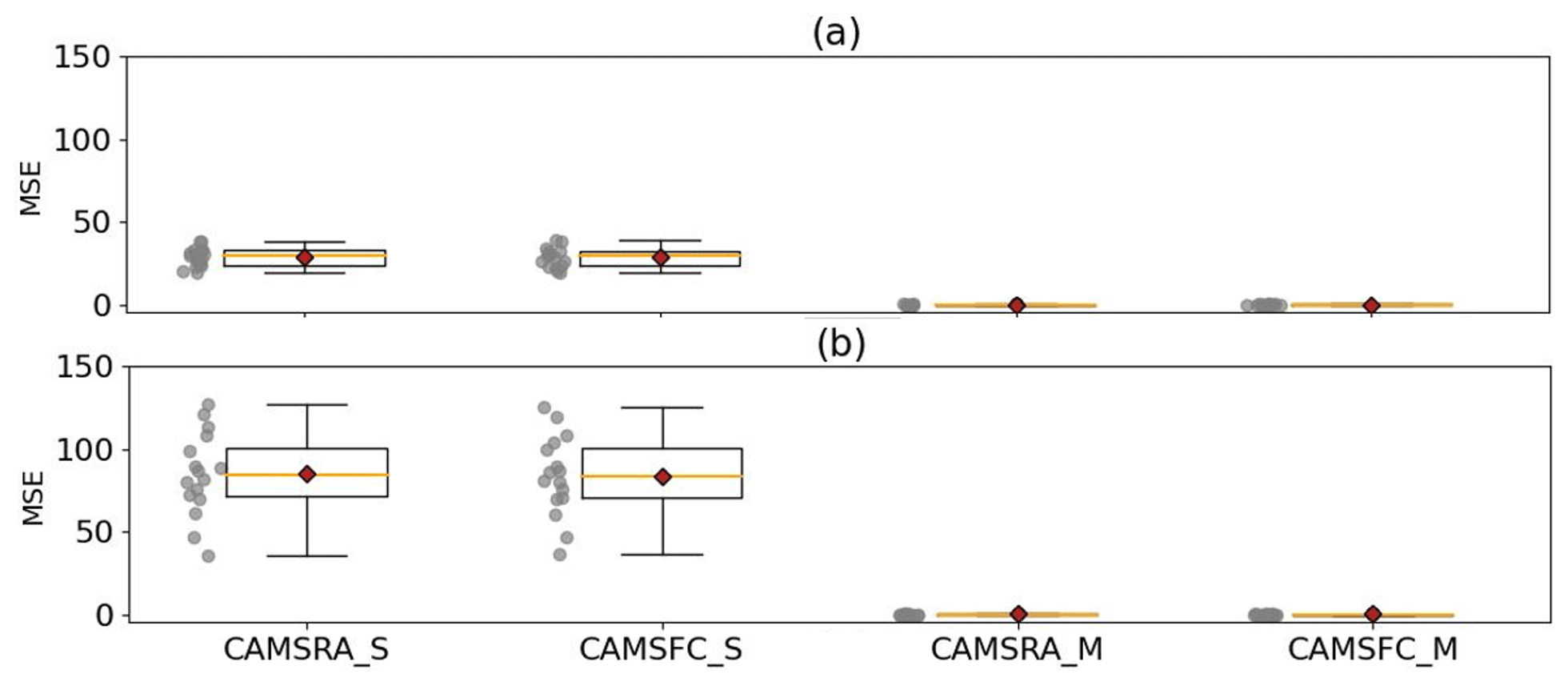
Figure A5The MSE of the O at the stations over Tehran city for (a) the cold (months 1–3 and 10–12) and (b) the warm (months 4–9) seasons.
Table A6The most important explanatory variables of the models at most of the stations.
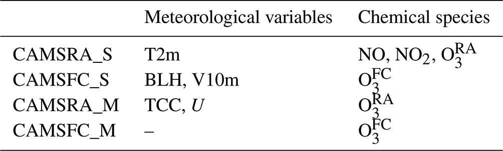
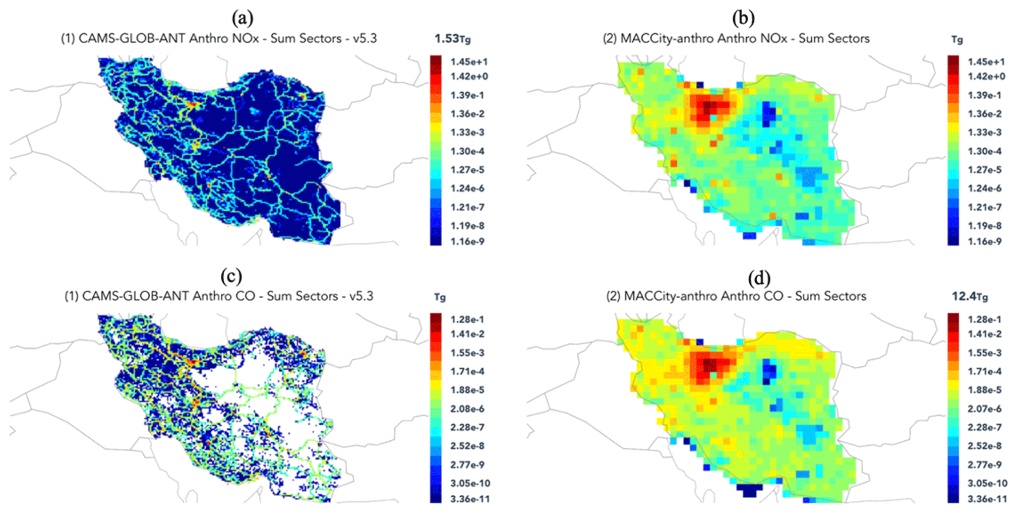
Figure A6The annual average of surface emissions of (a, b) NOx and (c, d) CO in the CAMS-GLOB-ANT and MACCity emission inventories.
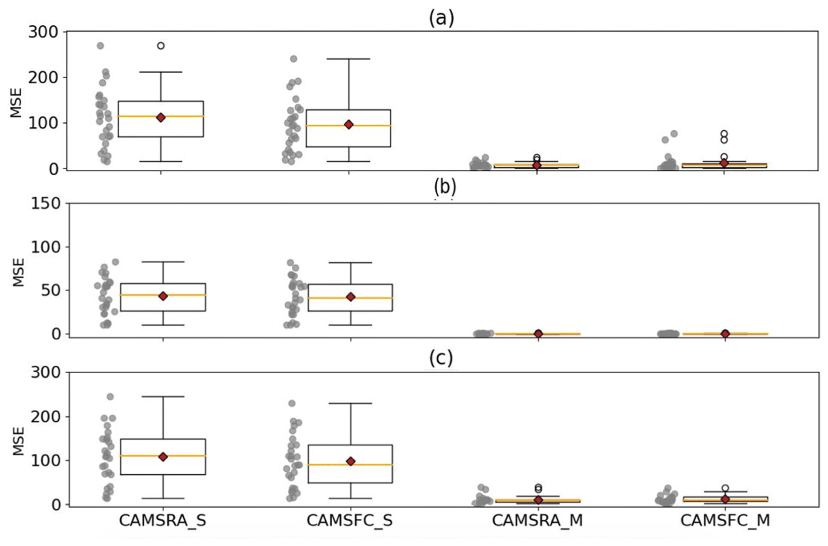
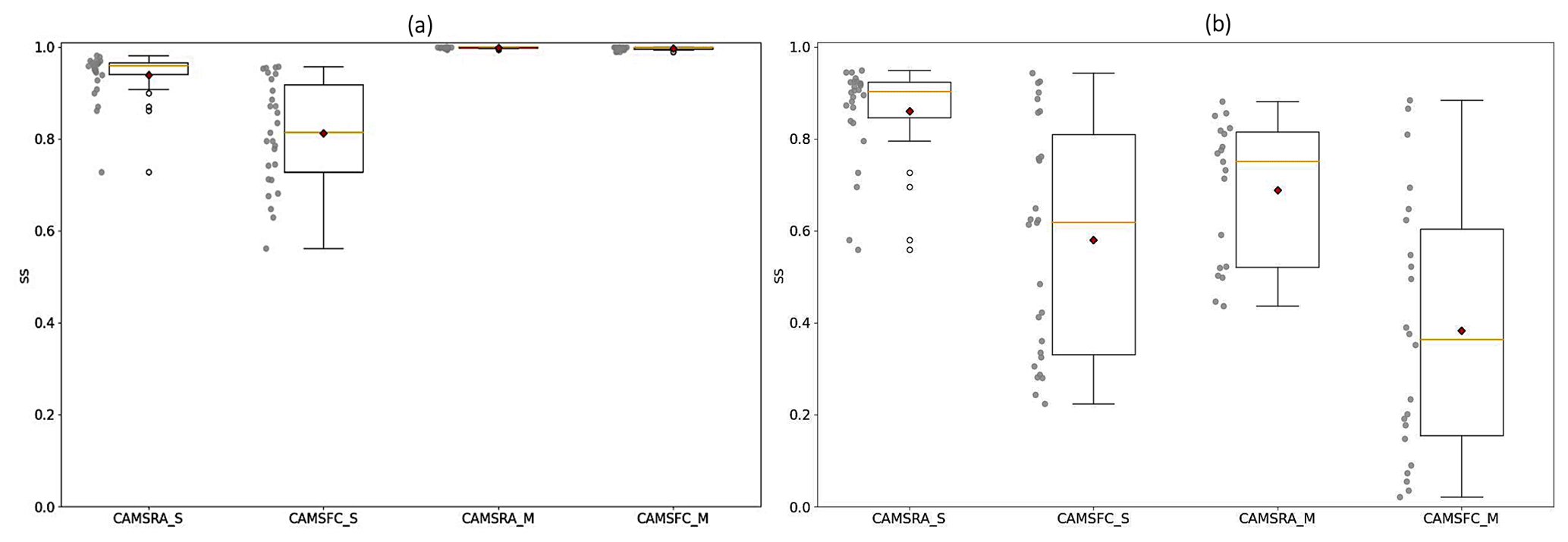
Table A7The results of the experiments (1) MLRno_lag (expr1): the model was trained only using O and O; and (2) MLRno_lag (expr2): the model was trained using the meteorological variables with high priority (listed in Table A6) at station 22 (Yazd). The r refers to the correlation coefficient between O and measured O3.
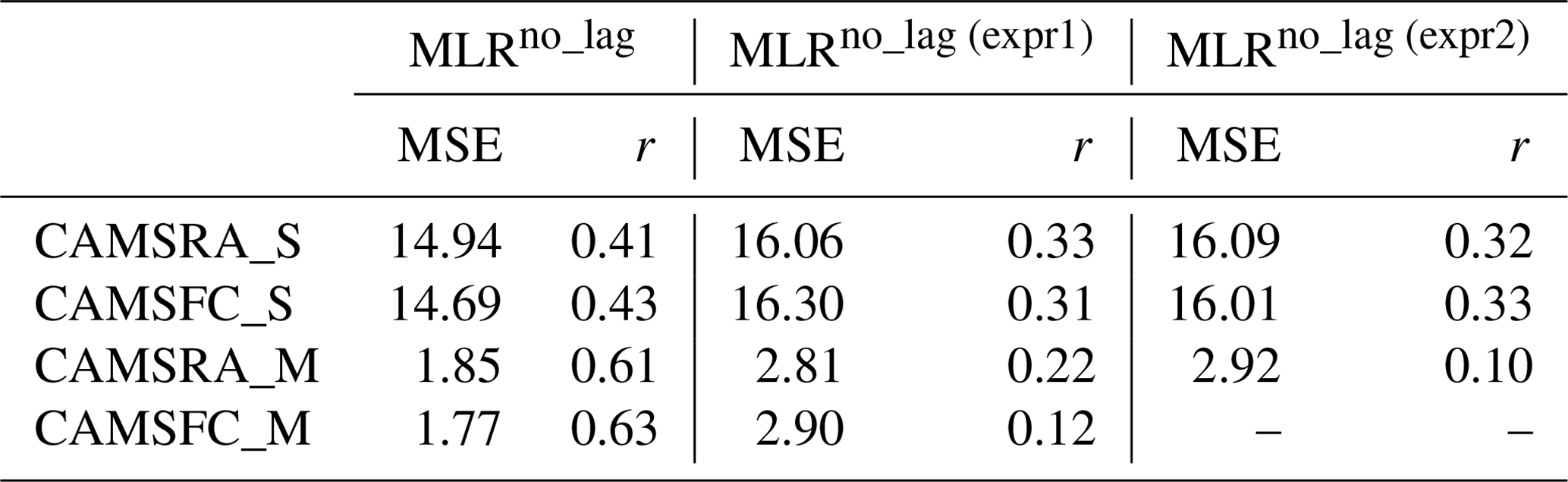
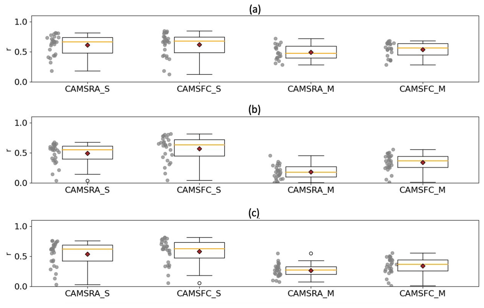
Figure A9The correlation (r) between measured O3 and O by the (a) MLRno_lag, (b) MLRno_lag (expr1), and (c) MLRno_lag (expr2) models.
The Python 3.7 code of the methodology and data are available at Zenodo (https://doi.org/10.5281/zenodo.10765491, Kaffashzadeh, 2024). Part of the observational data is accessible at https://airnow.tehran.ir (Air Quality Control Company, 2024). CAMS reanalysis and forecast datasets were obtained through ECMWF's atmospheric data service (https://ads.atmosphere.copernicus.eu/cdsapp#!/dataset/cams-global-reanalysis-eac4?tab=form, ECMWF, 2019).
NK designed the research, acquired and processed all data, performed the statistical analysis, and composed the figures and manuscript. AAAB contributed to proofreading.
The contact author has declared that neither of the authors has any competing interests.
Publisher's note: Copernicus Publications remains neutral with regard to jurisdictional claims made in the text, published maps, institutional affiliations, or any other geographical representation in this paper. While Copernicus Publications makes every effort to include appropriate place names, the final responsibility lies with the authors.
This study has been supported by the Center of International Science and Technology Cooperation (CISTC). We thank the data providers of the Iran Environmental Protection Organization, Tehran Air Quality Control Company, the ECMWF's climate data services, and the ECCAD. Appreciation is given to Martin Schultz for his help in training Najmeh Kaffashzadeh. Fabien Solmon is acknowledged for his valuable points during manuscript revisions. The authors highly acknowledge the constructive comments from two anonymous referees and the editor.
This paper was edited by Olaf Morgenstern and reviewed by two anonymous referees.
Ahmed, K., Shahid, S., Haroon, S. B., and Xiao-jun, W.: Multilayer perceptron neural network for downscaling rainfall in arid region: A case study of Baluchistan, Pakistan, J. Earth Syst. Sci., 124, 1325–1341, https://doi.org/10.1007/s12040-015-0602-9, 2015.
Air Quality Control Company (AQCC): Air Quality Control Company (AQCC) [data set], https://airnow.tehran.ir, last access: 17 May 2024.
Akritidis, D., Zanis, P., Pytharoulis, I., Mavrakis, A., and Karacostas, Th.: A deep stratospheric intrusion event down to the earth's surface of the megacity of Athens, Meteorol. Atmos. Phys., 109, 9–18, https://doi.org/10.1007/s00703-010-0096-6, 2010.
Akritidis, D., Pozzer, A., Zanis, P., Tyrlis, E., Škerlak, B., Sprenger, M., and Lelieveld, J.: On the role of tropopause folds in summertime tropospheric ozone over the eastern Mediterranean and the Middle East, Atmos. Chem. Phys., 16, 14025–14039, https://doi.org/10.5194/acp-16-14025-2016, 2016.
Aliakbari Bidokhti, A. A. and Shariepour, Z.: Analysis of surface ozone variability in the vicinity of synoptic (meteorology) station of Geophysics Institute (Tehran University) for the year 2002, J. Environ. Stud., 33, 63–74, 2007.
Asakereh, H. and Khojasteh, A.: Frequency of entrance Mediterranean Cyclones to Iran and Their Impact on Widespread precipitation, J. Nat. Environ. Hazards, 10, 159–176, https://doi.org/10.22111/jneh.2020.33171.1632, 2021.
Basart, S., Benedictow, A., Bennouna, Y., Blechschmidt, A.-M., Chabrillat, S., Christophe, Y., Cuevas, E., Eskes, H. J., Hansen, K. M., Jorba, O., Kapsomenakis, J., Langerock, B., Pay, T., Richter, A., Sudarchikova, N., Schulz, M., Wagner, A., and Zerefos, C.: Upgrade verification note for the CAMS real-time global atmospheric composition service: Evaluation of the e-suite for the CAMS upgrade of July 2019, Copernicus Atmosphere Monitoring Service (CAMS) report, 118 pp., https://doi.org/10.24380/fcwq-yp50, 2019.
Beecham, S., Rashid, M., and Chowdhury, R. K.: Statistical downscaling of multi-site daily rainfall in a South Australian catchment using a Generalized Linear Model, Int. J. Climatol., 34, 3654–3670, https://doi.org/10.1002/joc.3933, 2014.
Bell, M. L., Peng, R. D., and Dominici, F.: The Exposure – Response Curve for Ozone and Risk of Mortality and the Adequacy of Current Ozone Regulations, Environ. Health Perspect., 114, 532–536, https://doi.org/10.1289/ehp.8816, 2006.
Bidokhti, A. A., Shariepour, Z., and Sehatkashani, S.: Some resilient aspects of urban area to air pollution and climate change, case study: tehran, Iran, Scientia Iranica, 23, 1994–2005, 2016.
Bloomer, B. J., Stehr, J. W., Piety, C. A., Salawitch, R. J., and Dickerson, R. R.: Observed relationships of ozone air pollution with temperature and emissions, Geophys. Res. Lett., 36, 1–5, https://doi.org/10.1029/2009GL037308, 2009.
Borhani, F., Shafiepour Motlagh, M., Stohl, A., Rashidi, Y., and Ehsani, A. H.: Tropospheric Ozone in Tehran, Iran, during the last 20 years, Environ. Geochem. Health, 4, 3615–3637, https://doi.org/10.1007/s10653-021-01117-4, 2021.
Chen, Z., Liu, J., Qie, X., Cheng, X., Shen, Y., Yang, M., Jiang, R., and Liu, X.: Transport of substantial stratospheric ozone to the surface by a dying typhoon and shallow convection, Atmos. Chem. Phys., 22, 8221–8240, https://doi.org/10.5194/acp-22-8221-2022, 2022.
Chollet, F., et al.: Keras, GitHub [code], https://github.com/fchollet/keras (last access: 15 May 2024), 2015.
Cooper, O. R., Parrish, D. D., Ziemke, J., Balashov, N. V., Cupeiro, M., Galbally, I. E., Gilge, S., Horowitz, L., Jensen, N. R., Lamarque, J.-F., Naik, V., Oltmans, S. I., Schwab, J., Shindell, D. T., Thompson, A. M., Thouret, V., Wang, Y., and Zbinden, R. M.: Global distribution and trends of tropospheric ozone: An observation-based review, Elementa Sci. Anthropocene, 2, 000029, https://doi.org/10.12952/journal.elementa.000029, 2014.
Crutzen, P. J.: Photochemical reactions initiated by and influencing ozone in unpolluted tropospheric air, Tellus, 26, 47–57, https://doi.org/10.3402/tellusa.v26i1-2.9736, 1974.
ECMWF: CAMS global reanalysis (EAC4), ECMWF [data set], https://ads.atmosphere.copernicus.eu/cdsapp#!/dataset/cams-global-reanalysis-eac4?tab=form (last access: 17 May 2024), 2019.
Errera, Q., Bennouna, Y., Schulz, M., Eskes, H. J., Basart, S., Benedictow, A., Blechschmidt, A.-M., Chabrillat, S., Clark, H., Cuevas, E., Flentje, H., Hansen, K. M., Im, U., Kapsomenakis, J., Langerock, B., Petersen, K., Richter, A., Sudarchikova, N., Thouret, V., Wagner, A., Wang, Y., Warneke, T., and Zerefos, C.: Validation report of the CAMS global Reanalysis of aerosols and reactive gases, years 2003-2020, Copernicus Atmosphere Monitoring Service (CAMS) report, CAMS84_2018SC3_ D5.1.1-2020.pdf, https://doi.org/10.24380/8gf9-k005, 206 pp., June 2021.
Eskes, H. J., Basart, S., Benedictow, A., Bennouna, Y., Blechschmidt, A.-M., Errera, Q., Hansen, K. M., Kapsomenakis, J., Langerock, B., Richter, A., Sudarchikova, N., Schulz, M., and Zerefos, C.: Upgrade verification note for the CAMS near-real time global atmospheric composition service: Evaluation of the e-suite for the CAMS 47R3 upgrade of 12 October 2021, Copernicus Atmosphere Monitoring Service (CAMS) report, https://doi.org/10.24380/hfvp-fq98, 91 pp., October 2021.
Eskridge, R. E., Ku, J. Y., Rao, S. T., Porter, P. S., and Zurbenko, I. G.: Separating Different Scales of Motion in Time Series of Meteorological Variables, B. Am. Meteorol. Soc., 78, 7, 1473–1484, https://doi.org/10.1175/1520-0477(1997)078<1473:SDSOMI>2.0.CO;2, 1997.
Faridi, S., Shamsipour, M., Krzyzanowski, M., Künzli, N., Amini, H., Azimi, F., Malkawi, M., Momeniha, F., Gholampour, A., Hassanvand, M. S., and Naddafi, K.: Long-term trends and health impact of PM2.5 and O3 in Tehran, Iran, 2006–2015, Environ. Int., 114, 37–49, https://doi.org/10.1016/j.envint.2018.02.026, 2018.
Fiore, A. M., Jacob, D. J., Mathur, R., and Martin, R. V.: Application of empirical orthogonal functions to evaluate ozone simulations with regional and global models, J. Geophys. Res., 108, 4431, https://doi.org/10.1029/2002JD003151, 2003.
Flemming, J., Huijnen, V., Arteta, J., Bechtold, P., Beljaars, A., Blechschmidt, A.-M., Diamantakis, M., Engelen, R. J., Gaudel, A., Inness, A., Jones, L., Josse, B., Katragkou, E., Marecal, V., Peuch, V.-H., Richter, A., Schultz, M. G., Stein, O., and Tsikerdekis, A.: Tropospheric chemistry in the Integrated Forecasting System of ECMWF, Geosci. Model Dev., 8, 975–1003, https://doi.org/10.5194/gmd-8-975-2015, 2015.
Fowler, D., Pilegaard, K., Sutton, M. A., Ambus, P., Raivonen, M., Duyzer, J., Simpson, D., Fagerli, H., Fuzzi, S., Schjoerring, J. K., Granier, C., Neftel, A., Isaksen, I. S. A., Laj, P., Maione, M., Monks, P. S., Burkhardt, J., Daemmgen, U., Neirynck, J., Per- sonne, E., Wichink-Kruit, R., Butterbach-Bahl, K., Flechard, C., Tuovinen, J. P., Coyle, M., Gerosa, G., Loubet, B., Altimir, N., Gruenhage, L., Ammann, C., Cieslik, S., Paoletti, E., Mikkelsen, T. N., Ro-Poulsen, H., Cellier, P., Cape, J. N., Horvath, L., Loreto, F., Niinemets, U., Palmer, P. I., Rinne, J., Misztal, P., Nemitz, E., Nilsson, D., Pryor, S., Gallagher, M. W., Vesala, T., Skiba, U., Brueggemann, N., Zechmeister-Boltenstern, S., Williams, J., O'Dowd, C., Facchini, M. C., de Leeuw, G., Floss- man, A., Chaumerliac, N., and Erisman, J. W.: Atmospheric com- position change: Ecosystems-Atmosphere interactions, Atmos. Environ., 43, 5193–5267, https://doi.org/10.1016/j.atmosenv.2009.07.068, 2009.
Gandin, L. S.: Complex Quality Control of Meteorological Observations, Mon. Weather Rev., 116, 1137–1156, 460 https://doi.org/10.1175/1520-0493(1988)116<1137:CQCOMO>2.0.CO;2, 1988.
Gerharz, L., Gräler, B., and Pebesma, E.: Measurement artefacts and inhomogeneity detection, technical report, Uni. Münster, Germany, under subcontract of ETC/ACM Consortium institute RIVM, ETC/ACM, 54 pp., 2011.
Goudarzi, G., Geravandi., S., Foruozandeh, H., Babaei, A. A., Alavi, N., Niri, M. V., Khodayar, M. J., Salmanzadeh, S., and Mohammadi, M. J.: Cardiovascular and respiratory mortality attributed to ground-level ozone in Ahvaz, Iran, Environ. Monit. Assess., 187, 487, https://doi.org/10.1007/s10661-015-4674-4, 2015.
Granier, C., Bessagnet, B., Bond, T., D'Angiola, A., Denier van der Gon, H., Frost, G. J., Heil, A., Kaiser, J. W., Kinne, S., Klimont, Z., Kloster, S., Lamarque, J.-F., Liousse, C., Masui, T., Meleux, F., Mieville, A., Ohara, R., Raut, J.-C., Riahi, K., Schultz, M. G., Smith, S. G., Thompson, A., van Aardenne, J., van der Werf, G. R., and van Vuuren, D. P.: Evolution of anthropogenic and biomass burning emissions of air pollutants at global and regional scales during the 1980–2010 period, Clim. Change, 109, 163–190, https://doi.org/10.1007/s10584-011-0154-1, 2011.
Granier, C., Darras, S., Denier van der Gon, H. A. C., Doubalova, J., Elguindi, N., Galle, B., Gauss, M., Guevara, M., Jalkanen, J.-P., Kuenen, J., Liousse, C., Quack, B., Simpson, D., and Sindelarova, K.: The Copernicus Atmosphere Monitoring Service global and regional emissions (April 2019 version), Copernicus Atmosphere Monitoring Service (CAMS) report, 54 pp., https://doi.org/10.24380/d0bn-kx16, 2019.
Guenther, A., Karl, T., Harley, P., Wiedinmyer, C., Palmer, P. I., and Geron, C.: Estimates of global terrestrial isoprene emissions using MEGAN (Model of Emissions of Gases and Aerosols from Nature), Atmos. Chem. Phys., 6, 3181–3210, https://doi.org/10.5194/acp-6-3181-2006, 2006.
Hadei, M., Hopke, P. K., Nazari, S. S. H., Yarahmadi, M., Shahsavani, A., and Alipour, M. R.: Estimation of mortality and hospital admissions attributed to criteria air pollutants in Tehran metropolis, Iran (2013–2016), Aerosol Air Qual. Res., 17, 2474–2481, https://doi.org/10.4209/aaqr.2017.04.0128, 2017.
Haiden, T., Janousek, M., Vitart, F., Ferranti, L., and Prates, F.: Evaluation of ECMWF forecasts, including the 2019 upgrade, ECMWF Technical Memoranda No. 853, 54 pp., 2019.
Hochreiter, S. and Schmidhuber, J.: Long Short-Term Memory, Neural Computation, 9, 8, 1735–1780, 1997.
Hogrefe, C., Rao, S. T., Zurbenko, I. G., and Porter, P. S.: Interpreting the Information in Ozone Observations and Model Predictions Relevant to Regulatory Policies in the Eastern United States, B. Am. Meteorol. Soc., 8, 9, 2083–2106, 2000.
Hogrefe, C., Roselle, S., Mathur, R., Rao, S. T., and Galmarini, S.: Space-time analysis of the Air Quality Model Evaluation International Initiative (AQMEII) Phase 1 air quality simulations, J. Air Waste Manag. Assoc., 64, 388–405, https://doi.org/10.1080/10962247.2013.811127, 2014.
Hosseini, V. and Shahbazi, H.: Urban Air Pollution in Iran. Iranian Studies, 49, 6, 1029-1046, https://doi.org/10.1080/00210862.2016.1241587, 2016.
Huijnen, V., Williams, J., van Weele, M., van Noije, T., Krol, M., Dentener, F., Segers, A., Houweling, S., Peters, W., de Laat, J., Boersma, F., Bergamaschi, P., van Velthoven, P., Le Sager, P., Eskes, H., Alkemade, F., Scheele, R., Nédélec, P., and Pätz, H.-W.: The global chemistry transport model TM5: description and evaluation of the tropospheric chemistry version 3.0, Geosci. Model Dev., 3, 445–473, https://doi.org/10.5194/gmd-3-445-2010, 2010.
Huijnen, V., Miyazaki, K., Flemming, J., Inness, A., Sekiya, T., and Schultz, M. G.: An intercomparison of tropospheric ozone reanalysis products from CAMS, CAMS interim, TCR-1, and TCR-2, Geosci. Model Dev., 13, 1513–1544, https://doi.org/10.5194/gmd-13-1513-2020, 2020.
Inness, A., Ades, M., Agustí-Panareda, A., Barré, J., Benedictow, A., Blechschmidt, A.-M., Dominguez, J. J., Engelen, R., Eskes, H., Flemming, J., Huijnen, V., Jones, L., Kipling, Z., Massart, S., Parrington, M., Peuch, V.-H., Razinger, M., Remy, S., Schulz, M., and Suttie, M.: The CAMS reanalysis of atmospheric composition, Atmos. Chem. Phys., 19, 3515–3556, https://doi.org/10.5194/acp-19-3515-2019, 2019.
Jafari Hombari, F. and Pazhoh, F.: Synoptic analysis of the most durable pollution and clean waves during 2009–2019 in Tehran City (capital of Iran), Nat. Hazards, 110, 1247–1272, https://doi.org/10.1007/s11069-021-04990-5, 2022.
Kaffashzadeh, N.: A Statistical Analysis of Surface Ozone Variability Over the Mediterranean Region During Summer, Ph.D. thesis, Rheinishe Friedrich-Wilhelms-Universität Bonn, Germany, https://nbn-resolving.org/urn:nbn:de:hbz:5n-52000 (last access: 15 May 2024), 130 pp., 2018.
Kaffashzadeh, N.: Code and data archive for paper “Assessment of surface ozone products from downscaled CAMS reanalysis and CAMS daily forecast using urban air quality monitoring stations in Iran” (Version v2), Zenodo [code and data set], https://doi.org/10.5281/zenodo.10765491, 2024.
Kaffashzadeh, N. and Aliakbari Bidokhti, A. A.: Temporal variability analysis of measured surface ozone at the Geophysics Institute Station of the University of Tehran, J. Earth Space Phys., 48, 673–691, https://doi.org/10.22059/jesphys.2022.329346.1007355, 2022.
Kaiser, J. W., Heil, A., Andreae, M. O., Benedetti, A., Chubarova, N., Jones, L., Morcrette, J.-J., Razinger, M., Schultz, M. G., Suttie, M., and van der Werf, G. R.: Biomass burning emissions estimated with a global fire assimilation system based on observed fire radiative power, Biogeosciences, 9, 527–554, https://doi.org/10.5194/bg-9-527-2012, 2012.
Kang, D., Hogrefe, C., Foley, K. L., Napelenok, S. L., Mathur, R., and Rao, S. T.: Application of the Kolmogorov Zurbenko filter and the decoupled direct 3D method for the dynamic evaluation of a regional air quality model, Atmos. Environ., 80, 58–69, https://doi.org/10.1016/j.atmosenv.2013.04.046, 2013.
Khansalari, S., Ghobadi, N., Aliakbari Bidokhti, A., and Fazel Rastgar, F.: Statistical classification of synoptic weather patterns associated with Tehran air pollution, J. Air Pollut. He., 5, 43–62, https://doi.org/10.18502/japh.v5i1.2858, 2020.
Kilsby, C. G., Jones, P., Burton, A., Ford, A., Fowler, H. J., Harpham, C., James, P., Smith, A., and Wilby, R.: A daily weather generator for use in climate change studies, Environ. Model. Softw., 22, 1705–1719, https://doi.org/10.1016/j.envsoft.2007.02.005, 2007.
Lashkari, H., Keikhosravi, G., and Karimian, N.: Investigating Patterns of Severe Air Pollution in the Lower Tropospheric Layer of Tehran Metropolish, J. Geogr. Environ. Hazards, 9, 1–20, https://doi.org/10.22067/geo.v9i3.87260, 2020.
Lelieveld, J., Hoor, P., Jöckel, P., Pozzer, A., Hadjinicolaou, P., Cammas, J.-P., and Beirle, S.: Severe ozone air pollution in the Persian Gulf region, Atmos. Chem. Phys., 9, 1393–1406, https://doi.org/10.5194/acp-9-1393-2009, 2009.
Li, K., Jacob, D. J., Shen, L., Lu, X., De Smedt, I., and Liao, H.: Increases in surface ozone pollution in China from 2013 to 2019: anthropogenic and meteorological influences, Atmos. Chem. Phys., 20, 11423–11433, https://doi.org/10.5194/acp-20-11423-2020, 2020.
Loneck, B. and Zurbenko, I.: Theoretical and Practical Limits of Kolmogorov-Zurbenko Periodograms with DiRienzo-Zurbenko Algorithm Smoothing in the Spectral Analysis of Time Series Data Barry, arXiv [preprint], 28 pp., arXiv:2007.03031v1, 2020.
Malley, C. S., Heal, M. R., Mills, G., and Braban, C. F.: Trends and drivers of ozone human health and vegetation impact metrics from UK EMEP supersite measurements (1990–2013), Atmos. Chem. Phys., 15, 4025–4042, https://doi.org/10.5194/acp-15-4025-2015, 2015.
Michou, M., Laville, P., Serça, D., Fotiadi, A., Bouchou, P., and Peuch, V.-H.: Measured and modeled dry deposition velocities over the ESCOMPTE area, Atmos. Res., 74, 89–116, 2004.
Millaìn, M. M., Mantilla, E., Salvador, R., Carratalaì, R., Sanz, M. J., Alonso, L., Gangioti, G., and Navazo, M.: Ozone cycles in the Western Mediterranean basin: interpretation of monitoring data in complex coastal terrain, J. Appl. Meteorol., 39, 487–508, 2000.
Mills, G., Hayes, F., Simpson, D., Emberson, L., Norris, D., Har- mens, H., and Büker, P.: Evidence ofwidespread effects ofozone on crops and (semi-)natural vegetation in Europe (1990–2006) in relation to AOT40-and flux-based risk maps, Global. Change. Biol., 17, 592–613, https://doi.org/10.1111/j.1365-2486.2010.02217.x, 2011.
Monks, P. S.: A review of the observations and origins of the spring ozone maximum, Atmos. Environ., 34, 3545–3561, https://doi.org/10.1016/S1352-2310(00)00129-1, 2000.
Monks, P. S., Archibald, A. T., Colette, A., Cooper, O., Coyle, M., Derwent, R., Fowler, D., Granier, C., Law, K. S., Mills, G. E., Stevenson, D. S., Tarasova, O., Thouret, V., von Schneidemesser, E., Sommariva, R., Wild, O., and Williams, M. L.: Tropospheric ozone and its precursors from the urban to the global scale from air quality to short-lived climate forcer, Atmos. Chem. Phys., 15, 8889–8973, https://doi.org/10.5194/acp-15-8889-2015, 2015.
Mughal, M. O., Lynch, M., Yu, F., McGann, B., Jeanneret, F., and Sutton, J.: Wind modelling, validation and sensitivity study using Weather Research and Forecasting model in complex terrain, Environ. Model. Softw., 90, 107–125, https://doi.org/10.1016/j.envsoft.2017.01.009, 2017.
Murphy, A. H.: Skill Scores Based on the Mean Square Error and Their Relationships to the Correlation Coefficient, Mon. Weather Rev., 116, 2417–2424, https://doi.org/10.1175/1520-0493(1988)116<2417:SSBOTM>2.0.CO;2, 1988.
Park, S., Son, S. W., Jung, M. Il, Park, J., and Park, S. S.: Evaluation of tropospheric ozone reanalyses with independent ozonesonde observations in East Asia, Geosci. Lett., 7, 12, https://doi.org/10.1186/s40562-020-00161-9, 2020.
Pozzer, A., Anenberg, S. C., Dey, S., Haines, A., Lelieveld, J., and Chowdhury, S.: Mortality attributable to ambient air pollution: A review of global estimates, GeoHealth, 7, 1–25, https://doi.org/10.1029/2022GH000711, 2023.
Rao, S. T., Zurbenko, I. G., Neagu, R., Porter, P. S., Ku, J. Y., and Henry, R. F.: Space and Time Scales in Ambient Ozone Data, B. Am. Meteorol. Soc., 78, 2153–2166, https://doi.org/10.1175/1520-0477(1997)078<2153:SATSIA>2.0.CO;2, 1997.
Sachindra, D. A., Huang, F., Barton, A. F., and Perera, B. J. C.: Least square support vector and multi-linear regression for statistically downscaling general circulation model outputs to catchment streamflows, Int. J. Climatol., 33, 1087–1106, https://doi.org/10.1002/joc.3493, 2013.
Sachindra, D. A., Ahmed, K., Mamunur Rashid, Md., Shahid, S., and Perera, B. J. C.: Statistical downscaling of precipitation using machine learning techniques, Atmos. Res., 212, 240–258, https://doi.org/10.1016/j.atmosres.2018.05.022, 2018.
Schulz, M., Errera, Q., Ramonet, M., Sudarchikova, N., Eskes, H. J., Basart, S., Benedictow, A., Bennouna, Y., Blechschmidt, A.-M., Chabrillat, S., Christophe, Y., Cuevas, E. El-Yazidi, A., Flentje, H., Fritzsche, P., Hansen, K. M., Im, U., Kapsomenakis, J., Langerock, B., Richter, A., Thouret, V., Wagner, A., Warneke, T., and Zerefos, C.: Validation report of the CAMS near-real-time global atmospheric composition service: Period December 2020 – February 2021, Copernicus Atmosphere Monitoring Service (CAMS) report, CAMS84_2018SC3_D1.1.1_DJF2021.pdf, https://doi.org/10.24380/f540-kb09, 190 pp., June 2021.
Sebbar, B. E., Khabba, S., Merlin, O., Simonneaux, V., Hachimi, C. E., Kharrou M. H., and Chehbouni, A.: Machine-Learning-Based Downscaling of Hourly ERA5-Land Air Temperature over Mountainous Regions, Atmosphere, 14, 610, https://doi.org/10.3390/atmos14040610, 2023.
Semenov, M. A. and Stratonovitch, P.: Use of multi-model ensembles from global climate models for assessment of climate change impacts, Climate Res., 41, 1–14, 2010.
Seo, J., Youn, D., Kim, J. Y., and Lee, H.: Extensive spatiotemporal analyses of surface ozone and related meteorological variables in South Korea for the period 1999–2010, Atmos. Chem. Phys., 14, 6395–6415, https://doi.org/10.5194/acp-14-6395-2014, 2014.
Shahbazi, H., Mostafazade Abolmaali, A., Alizadeh, H., Salavati, H., Zokaei, H., Zandavi, R., Torbatian, S., Yazgi, D., and Hosseini, V.: An emission inventory update for Tehran: The difference between air pollution and greenhouse gas source contributions, Atmos. Res., 275, 106240, https://doi.org/10.1016/j.atmosres.2022.106240, 2022.
Sharipour, Z. and Aliakbari Bidokhti, A. A.: Investigation of spatial and temporal distributions of air pollutants over Tehran in cold months of 2011–2013, J. Environ. Sci. Technol., 16, 149–166, 2014.
Shariepour, Z. and Aliakbari Bidokhti, A. A.: Investigation of Surface Ozone over Tehran for 2008–2011, J. Earth Space Phys., 39, 191–206, https://doi.org/10.22059/jesphys.2013.35607, 2013.
Sillman, S. and Samson, P. J.: Impact of temperature on oxidant photochemistry in urban, polluted rural and remote environments, J. Geophys. Res., 100, 11497–11508, https://doi.org/10.1029/94JD02146, 1995.
Sindelarova, K., Granier, C., Bouarar, I., Guenther, A., Tilmes, S., Stavrakou, T., Müller, J.-F., Kuhn, U., Stefani, P., and Knorr, W.: Global data set of biogenic VOC emissions calculated by the MEGAN model over the last 30 years, Atmos. Chem. Phys., 14, 9317–9341, https://doi.org/10.5194/acp-14-9317-2014, 2014.
Sindelarova, K., Markova, J., Simpson, D., Huszar, P., Karlicky, J., Darras, S., and Granier, C.: High-resolution biogenic global emission inventory for the time period 2000–2019 for air quality modelling, Earth Syst. Sci. Data, 14, 251–270, https://doi.org/10.5194/essd-14-251-2022, 2022.
Solazzo, E. and Galmarini, S.: Error apportionment for atmospheric chemistry-transport models – a new approach to model evaluation, Atmos. Chem. Phys., 16, 6263–6283, https://doi.org/10.5194/acp-16-6263-2016, 2016.
Stein, O., Schultz, M. G., Bouarar, I., Clark, H., Huijnen, V., Gaudel, A., George, M., and Clerbaux, C.: On the wintertime low bias of Northern Hemisphere carbon monoxide found in global model simulations, Atmos. Chem. Phys., 14, 9295–9316, https://doi.org/10.5194/acp-14-9295-2014, 2014.
Steinacker, R., Mayer, D., and Steiner, A.: Data Quality Control Based on Self-Consistency, Mon. Weather Rev., 139, 3974–3991, https://doi.org/10.1175/MWR-D-10-05024.1, 2011.
Stull, R. B.: An Introduction to Boundary Layer Meteorology, Springer Science & Business Media, 13, 670 pp., 1988.
Sudarchikova, N., Schulz, M., Errera, Q., Ramonet, M., Eskes, H. J., Basart, S., Benedictow, A., Bennouna, Y., Blechschmidt, A.-M., Chabrillat, S., Christophe, Y., Cuevas, E., El-Yazidi, A., Flentje, H., Fritzsche, P., Hansen, K. M., Im, U., Kapsomenakis, J., Langerock, B., Richter, A., Thouret, V., Wagner, A., Warneke, T., and Zerefos, C.: Validation report of the CAMS near-real-time global atmospheric composition service: Period September - November 2020, Copernicus Atmosphere Monitoring Service (CAMS) report, CAMS84_2018SC3_D1.1.1_SON2020.pdf, https://doi.org/10.24380/rysv-7371, 159 pp., March 2021.
Taylor, J. R. and Loescher, H. L.: Automated quality control methods for sensor data: a novel observatory approach, Biogeosciences, 10, 4957–4971, https://doi.org/10.5194/bg-10-4957-2013, 2013.
Tripathi, S., Srinivas, V. V., and Nanjundiah, R. S.: Downscaling of precipitation for climate change scenarios: a support vector machine approach, J Hydrol., 330, 621–640, https://doi.org/10.1016/j.jhydrol.2006.04.030, 2006.
Tyrlis, E., Lelieveld, J., and Steil, B.: The summer circulation over the eastern Mediterranean and the Middle East: influence of the South Asian monsoon, Clim. Dynam., 40, 1103–1123, https://doi.org/10.1007/s00382-012-1528-4, 2013.
Tyrlis, E., Skerlak, B., Sprenger, M., Wernli, H., Zittis, G., and Lelieveld, J.: On the linkage between the Asian summer mon- soon and tropopause fold activity over the eastern Mediterranean and the Middle East, J. Geophys. Res.-Atmos., 119, 3202–3221, 2014.
Velchev, K., Cavalli, F., Hjorth, J., Marmer, E., Vignati, E., Dentener, F., and Raes, F.: Ozone over the Western Mediterranean Sea – results from two years of shipborne measurements, Atmos. Chem. Phys., 11, 675–688, https://doi.org/10.5194/acp-11-675-2011, 2011.
Wagner, A., Bennouna, Y., Blechschmidt, A., Brasseur, G., Chabrillat, S., Christophe, Y., Errera, Q., Eskes, H., Flemming, J., Hansen, K. M., Inness, A., Kapsomenakis, J., Langerock, B., Richter, A., Sudarchikova, N., Thouret, V., and Zerefos, C.: Comprehensive evaluation of the Copernicus Atmosphere Monitoring Service (CAMS) reanalysis against independent observations: Reactive gases, Elem. Sci. Anth., 9, 1–31, https://doi.org/10.1525/elementa.2020.00171, 2021.
Wang, Y., Ma, Y.-F., Eskes, H., Inness, A., Flemming, J., and Brasseur, G. P.: Evaluation of the CAMS global atmospheric trace gas reanalysis 2003–2016 using aircraft campaign observations, Atmos. Chem. Phys., 20, 4493–4521, https://doi.org/10.5194/acp-20-4493-2020, 2020.
Wentworth, G. R., Murphy, J. G., and Sills, D. M. L.: Impact of lake breezes on ozone and nitrogen oxides in the greater toronto area, Atmos. Environ., 109, 52–60, https://doi.org/10.1016/j.atmosenv.2015.03.002, 2015.
Wilby, R. L. and Dawson, C. W.: The Statistical DownScaling Model: insights from one decade of application, Int. J. Climatol., 33, 1707–1719, https://doi.org/10.1002/joc.3544, 2013.
Wilby, R. L. and Wigley, T. M. L.: Downscaling general circulation model output: A review of methods and limitations, Prog. Phys. Geogr., 21, 530–548, https://doi.org/10.1177/030913339702100403, 1997.
Wilby, R. L., Charles, S. P., Zorita, E., Timbal, B., Whetton, P., and Mearns, L. O.: Guidelines for use of climate scenarios developed from statistical downscaling methods, supporting material to the IPCC, 3–21, https://www.ipcc-data.org/guidelines/dgm_no2_v1_09_2004.pdf (last access: 15 May 2024), 2004.
Wilks, D. S.: Multisite downscaling of daily precipitation with a stochastic weather generator, Clim. Res., 11, 125–136, 1999.
Wilks, D. S.: Statistical Methods in the Atmospheric Sciences, international Geophysics Series, 91, 649 pp., 2nd edn., 2006.
Yang, W. and Zurbenko, I.: Kolmogorov – Zurbenko filters, WIREs Comp. Stat., 2, 340–351, https://doi.org/10.1002/wics.71, 2010.
Yousefian, F., Faridi, S., Azimi, F., Aghaei, M., Shamsipour, M., Yaghmaeian, K., and Hassanvand, M. S.: Temporal variations of ambient air pollutants and meteorological influences on their concentrations in Tehran during 2012–2017, Sci. Rep., 10, 1–11, https://doi.org/10.1038/s41598-019-56578-6, 2020.
Zahumenský, I.: Guidelines on Quality Control Procedures for Data from Automatic Weather Stations Guidelines on Quality Control Procedures for Data from Automatic Weather Stations, World Meteorological Organization, 10 pp., 2004.
Zanis, P., Hadjinicolaou, P., Pozzer, A., Tyrlis, E., Dafka, S., Mihalopoulos, N., and Lelieveld, J.: Summertime free-tropospheric ozone pool over the eastern Mediterranean/Middle East, Atmos. Chem. Phys., 14, 115–132, https://doi.org/10.5194/acp-14-115-2014, 2014.
Zhang, J. and Rao, S. T.: The role of vertical mixing in the temporal evolution of ground- level ozone concentrations, J. Appl. Meteor. Climatol., 38, 1674–1691, https://doi.org/10.1175/1520-0450(1999)038<1674:TROVMI>2.0.CO;2, 1999.
Zohdirad, H., Montazeri Namin, M., Ashrafi, K., Aksoyoglu, S., and Prévôt, A. S. H.: Temporal variations, regional contribution, and cluster analyses of ozone and NOx in a middle eastern megacity during summertime over 2017–2019, Environ. Sci. Pollut. Res., 29, 16233–16249, https://doi.org/10.1007/s11356-021-14923-1, 2022.
Zurbenko, I., Porter, P. S., Gui, R., Rao, S. T., Ku, J. Y., and Eskridge, R. E.: Detecting discontinuities in time series of upper-air data: development and demonstration of an adaptive filter technique, J. Climate, 9, 3548–3560, https://doi.org/10.1175/1520-0442(1996)009<3548:DDITSO>2.0.CO;2, 1996.