A revised model of global silicate weathering considering the influence of vegetation cover on erosion rate

Silicate weathering, which is of great importance in regulating the global carbon cycle, has been found to be affected by complicated factors, including climate, tectonics and vegetation. However, the exact transfer function between these factors and the silicate weathering rate is still unclear, leading to large model–data discrepancies in the CO₂ consumption associated with silicate weathering. Here we propose a simple parameterization for the influence of vegetation cover on erosion rate to improve the model–data comparison based on a state-of-the-art silicate weathering model. We found out that the current weathering model tends to overestimate the silicate weathering fluxes in the tropical region, which can hardly be explained by either the uncertainties in climate and geomorphological conditions or the optimization of model parameters. We show that such an overestimation of the tropical weathering rate can be rectified significantly by parameterizing the shielding effect of vegetation cover on soil erosion using the leaf area index (LAI), the high values of which are coincident with the distribution of leached soils. We propose that the heavy vegetation in the tropical region likely slows down the erosion rate, much more so than thought before, by reducing extreme streamflow in response to precipitation. The silicate weathering model thus revised gives a smaller global weathering flux which is arguably more consistent with the observed value and the recently reconstructed global outgassing, both of which are subject to uncertainties. The model is also easily applicable to the deep-time Earth to investigate the influence of land plants on the global biogeochemical cycle.

1 Introduction

On geological timescales, Earth's climate is primarily controlled by the atmospheric CO₂ concentration (pCO₂); the evolution of the Sun – its brightness increases with time – also plays an important role on the timescale of a hundred million years (100 Myr) but in a temporally smooth way (Li et al., 2023). However, how the sources and sinks of CO₂ varied in Earth's history remains elusive (Y. Zhang et al., 2022; Mills et al., 2021), and large uncertainties exist even in the estimate of their present-day magnitudes (Hilton and West, 2020). Due to the small size of the ocean–atmosphere carbon reservoir (∼40 000 Pg; Lee et al., 2019; Berner, 2004; Canadell et al., 2023), a small imbalance between the carbon sources and sinks can lead to large variations in pCO₂ in a relatively short time (Berner and Kothavala, 2001; Berner, 1991; Walker et al., 1981; Berner, 2004). Therefore, accurately determining the exact magnitude of carbon sources and sinks is crucial for comprehensively understanding the mechanisms behind Earth's climate variations.

One of the essential ways of determining the carbon sink is through numerical modeling, especially for that in the deep past. Numerical models not only provide the magnitude of the carbon sink but also allow us to study its sensitivity to various factors such as continental evolution and climate change. Our goal here is to improve the model calculation of the primary sink of CO₂, i.e., the silicate weathering, with a focus on its present-day values for which the spatial distribution is relatively well constructed.

The rate of silicate weathering is affected by the composition and physical erosion of surface rocks, pCO₂, surface temperature and terrestrial runoff (Gaillardet et al., 1999; Raymo and Ruddiman, 1992; Brantley et al., 2008; Maher, 2010; Maher and Chamberlain, 2014; Dessert et al., 2003; Ibarra et al., 2019; West et al., 2005). Seawater isotopes such as Sr, Os, Li or Be are often used to estimate the global silicate weathering flux in the past (Caves Rugenstein et al., 2019; Dellinger et al., 2015; Kalderon-Asael et al., 2021; Li et al., 2019). However, it is difficult to constrain the sensitivity of silicate weathering to certain factors (e.g., temperature) from such measurements, especially in local regions, due to both the uncertainties in their interpretation (Li et al., 2019; Dellinger et al., 2015) and their global nature. Simulating the weathering reactions in the lab can provide useful information for the factors that control the weathering rate, but lab conditions are generally much simpler than those in the natural field (Gruber et al., 2014; Calabrese et al., 2022; White and Brantley, 2003). Many other works focused on compiling the dissolved river loading to estimate the silicate weathering fluxes and rates in different regions for the present day (Bluth and Kump, 1994; Gibbs et al., 1999; Amiotte Suchet et al., 2003; Suchet and Probst, 2002). Despite the various uncertainties in these methods, they provide a basis for the development of numerical models.

Early zero-dimensional models (e.g., the Geologic Carbon Cycle (GEOCARB) family; Walker et al., 1981; Berner et al., 1983; Berner, 1991) and subsequent two-dimensional numerical models such as the Gibbs and Kump Weathering Model (GKWM) in 1994 (Bluth and Kump, 1994), the Global Erosion Model for CO₂ fluxes (GEM-CO₂) in 1995 (Suchet and Probst, 2002; Amiotte Suchet et al., 2003) and a model by Jens Hartmann in 2009 (Hartmann et al., 2009; Hartmann and Moosdorf, 2012; Hartmann et al., 2014) provided important understanding of the long-term carbon cycle. Studies using these models (Amiotte Suchet et al., 2003; Gibbs et al., 1999; Zhang et al., 2021) have identified the lithology and runoff as the strongest predictors of chemical weathering rates. However, basin- or catchment-scale compilation of weathering data (Gaillardet et al., 1999) indicates that the spatial variability of the weathering rate had to be explained through a combined effect of runoff, temperature and erosion rate. West et al. (2005) further showed that there were two-end-member schemes of the weathering – transport-limited and kinetically limited regimes.

Built on the work of West et al. (2005), Gabet and Mudd (2009) constructed a theoretical model (referred to as the GM09 model hereafter) that encompassed the continuum of these two weathering regimes for the first time. This model is probably the most sophisticated one to date in terms of global silicate weathering calculation and has been used in many works subsequently for both the present day and the past (West, 2012; Goddéris et al., 2017; Maffre et al., 2018; Park et al., 2020). However, the model contains a few unknown parameters, including cation abundance in the bedrock, the dissolution rate constant and its dependence on runoff and reaction time, and the regolith production rate, of which only rough ranges are given. Most previous works (Maffre et al., 2018; Park et al., 2020) using this model estimated these parameters through some fitting approach with the help of catchment-scale observations (Gaillardet et al., 1999).

The global total silicate weathering flux (F_w) of the present day given by Park et al. (2020) (referred to as Park20 hereafter) in terms of carbon is $\sim \mathrm{4.5}\times {\mathrm{10}}^{\mathrm{12}}$ mol yr⁻¹, which was thought to be consistent with the global outgassing rate estimated by Gerlach (2011). However, a few lines of evidence indicate that this flux may be overestimated. (1) The F_w estimated from the present-day observations is $\sim \mathrm{2.5}\times {\mathrm{10}}^{\mathrm{12}}$ mol yr⁻¹ (1.59×10¹²–2.75×10¹² mol yr⁻¹) (Gaillardet et al., 1999; Moon et al., 2014). (2) The global outgassing rate was re-estimated to be ∼2–3.3×10¹² mol yr⁻¹ by Müller et al. (2022). (3) The silicate weathering fluxes for individual river basins within the tropical region from the Park20 model were overall overestimated compared to the observations (Fig. 1b), which led to an overestimate of F_w (Fig. 1c). This overestimation over the tropical region by the Park20 model has also been argued to exist based on the observed ${}^{\mathrm{187}}\mathrm{Os}{/}^{\mathrm{188}}\mathrm{Os}$ (Caves Rugenstein et al., 2021).

Overestimation of the carbon sink by 100 % will lead to a dramatic decrease in pCO₂ and an extreme icehouse climate in a few million years when the outgassing is fixed (Berner and Caldeira, 1997; D'Antonio et al., 2019) and thus should be dealt with properly. More important reasons may be that (1) the overestimation is not random among different sites but is systematic; the weathering fluxes over tropical river basins are much more likely overestimated than underestimated, whether in the original values (Fig. 1b) or in the logarithmic values (Fig. 1e). (2) The climate sensitivity of the silicate weathering, i.e., the ability of silicate weathering to stabilize the climate, may be mis-estimated due to this systematic error.

The lower-than-expected silicate weathering rate over the tropical region was noticed by Stallard as early as 1981 (Stallard and Edmond, 1981; Stallard, 1985; Stallard and Edmond, 1983). Godderis et al. (2008) and Hartmann et al. (2014) also found that considering only the effects of temperature and runoff would lead to a significant overestimation of weathering in the tropical region. They proposed the effect of soil shielding as a solution; i.e., the occurrence of leached soil in equatorial regions hinders deeper weathering. They then assumed a global soil shielding effect in regions with leached soil and improved their model performance. However, the soil shielding effect has already been considered in the GM09 model to some extent, where the physical erosion was parameterized. Therefore, the problem remains in this model, and our main goal in this paper is to find a simple solution to the problem and test whether it affects the sensitivity of global silicate weathering to climate change.

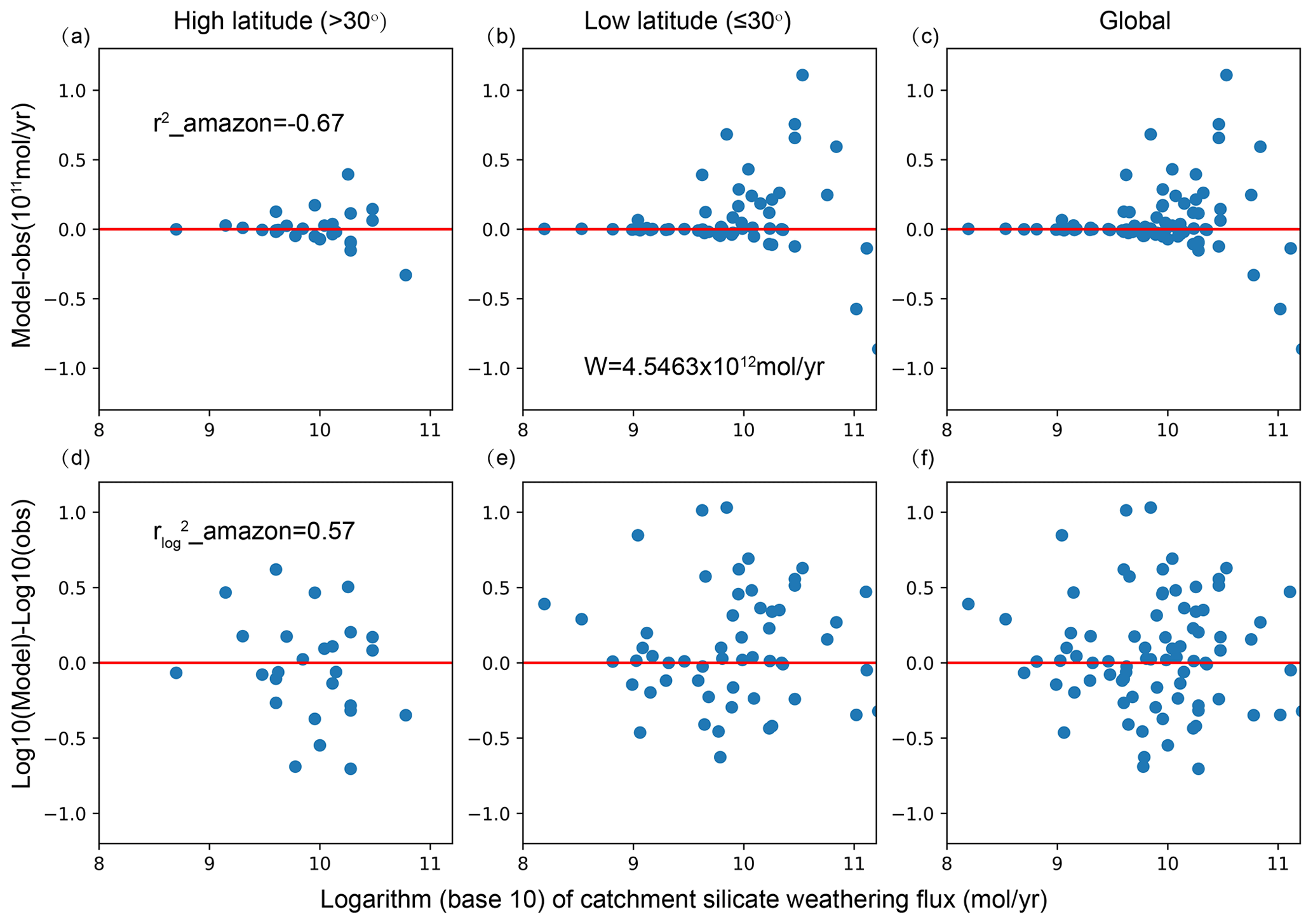
Figure 1 The difference between the model calculated and observed silicate weathering fluxes for 81 large rivers (more details can be found in Sect. 2.2.5) over the world. The upper and lower panels show model-obs and log₁₀(model)-log₁₀(obs), respectively. The left, middle and right panels show rivers at the mid to high latitudes (if more than half of its river basin is located at or beyond 30° latitude), low latitudes (within 30° latitude) and over the whole globe, respectively. The model results were calculated using the GM09 model but with model parameters in Park20. The global total weathering flux is 4.5×10¹² mol yr⁻¹. The surface slope and all climate forcings are from Park20, in which the runoff used is the one denoted as “from Yves” in Park20 (more details in Sect. 2.2.1). A similar systematic upward bias in the tropical region appeared when the parameters as given in Maffre et al. (2022) were used (Fig. S1 in the Supplement).

Specifically, we will first test whether the historical climate data constructed by different institutes have any significant impact on the calculated silicate weathering rate using the GM09 model in the tropical region. Then, the influence of the magnitude of the seasonal cycle on physical weathering is tested next. It is then found that reducing physical erosion rates where leached soil is present works best in removing the systematic bias in the tropical region. In the end, we find a simple parameterization scheme related to vegetation that can attain a similar effect to that of leached soil but that is much more applicable to weathering calculation for other periods of Earth's history.

The rest of the paper is organized as follows. In Sect. 2, the GM09 model is briefly described, and the field observations used to validate the model and climate data used to calculate the weathering fluxes are also described. In Sect. 3, the results of various sensitivity tests and the parameterization for the vegetation effect are presented. The shortcomings as well as the consequences of the model revision are then discussed in Sect. 4, and a summary is provided in Sect. 5.

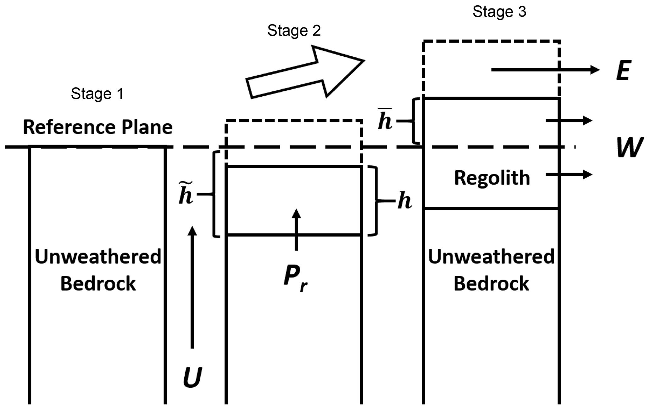
Figure 2 Schematic diagram of the theoretical model of bedrock weathering and the simultaneous production of soil or regolith based on GM09. In stage 1, the unweathered bedrock moves vertically at a speed U due to tectonic movement, with weathering and erosion just to occur at the surface. In stage 2, soil is produced (P_r) at the surface of the bedrock and eroded (E) at the soil top, with silicate weathering occurring mostly within the soil. h represents the soil thickness, and $\overline{h}$ and $\stackrel{\mathrm{̃}}{h}$ are the heights of the soil and the bedrock surface, respectively, relative to the reference plane (note that $\overline{h}$ is nonzero in stage 2 but is not marked for the sake of esthetics). The part enclosed by dashed lines is eroded away. All variables evolve with time at this stage. In stage 3, a steady state is reached under continuous weathering such that the soil thickness and the weathering flux do not change with time anymore. The weathered material within the soil is carried away by water runoff into the oceans, with the weathering flux denoted as W.

2 Model and data

2.1 Theoretical model for silicate weathering

2.1.1 The weathering profile and weathering flux

For the convenience of the latter discussion, the model GM09 as presented in detail in Park20 and Maffre et al. (2022) is recapped here. The model includes an explicit simulation of a regolith layer, which extends from the soil surface to the unweathered bedrock (Fig. 2). The layer can be millimeters to tens of meters thick depending on the environment and is determined by

$$\begin{array}{}\text{(1)}& {\displaystyle \frac{\mathrm{d}h}{\mathrm{d}t}}={\displaystyle \frac{\mathrm{d}\stackrel{\mathrm{̃}}{h}}{\mathrm{d}t}}+{\displaystyle \frac{\mathrm{d}\overline{h}}{\mathrm{d}t}}=P_{\mathrm{r}}-U+U-E=P_{\mathrm{r}}-E,\end{array}$$

where h is the regolith thickness, P_r is the soil production rate and E is the erosion rate. The weathering rate J at depth z is proportional to the concentration of cations (e.g., Ca²⁺ and Mg²⁺) denoted as x and also depends on the temperature (T), runoff (q) and exposure time (τ) that the sample has experienced. The influences of T and q are generally considered using the Arrhenius equation and a linear or power-law relation (White and Blum, 1995; Dessert et al., 2003), respectively. When an exponential dependence of the weathering rate on runoff q is employed as in Park20, the weathering rate J is written as

$$\begin{array}{}\text{(2)}& J\left(z\right)=K\cdot (\mathrm{1}-e^{-k_{\mathrm{w}}\cdot q})\cdot e^{-\frac{E_{\mathrm{a}}}{R}\cdot \left(\frac{\mathrm{1}}{T}-\frac{\mathrm{1}}{T_{\mathrm{0}}}\right)}\cdot {\mathit{\tau }}^{\mathit{\sigma }}\cdot x\left(z\right),\end{array}$$

where K is the dissolution constant, k_w is the runoff sensitivity of the dissolution rate, E_a is the apparent activation energy at T₀ for dissolution, R is the gas constant, and σ is an empirical constant.

It should be noted that the global total silicate weathering flux throughout this work pertains specifically to the weathering flux of Ca and Mg silicates. While Na and K silicates also participate in weathering, these are not traditionally regarded as carbon sinks on geological timescales (Berner et al., 1983) due to their inability to form carbonate minerals. However, the residence times of Na⁺ and K⁺ in the ocean are ∼80 and ∼10 Myr (Lécuyer, 2016; Emerson and Hedges, 2008; Olson et al., 2022; Berner and Berner, 2012; Hu et al., 2020), respectively. This long residence time means that the weathering of Na and K silicates could have an impact on the atmospheric CO₂ on a 1 million year timescale. Moreover, Na⁺ and K⁺, when released into the soil through weathering reactions, may displace Ca²⁺ and Mg²⁺ through cation exchange with sediments or oceanic crust (France-Lanord and Derry, 1997), leading to carbonate deposition and carbon sinking indirectly. However, currently we are unable to quantify these aspects due to the intricacies of the Na and K cycles. Thus, we focus solely on the Ca²⁺ and Mg²⁺ silicate weathering flux in the current study.

The concentration of cations themselves changes with time according to

$$\begin{array}{}\text{(3)}& {\displaystyle \frac{\partial x}{\partial t}}=-U\cdot {\displaystyle \frac{\partial x}{\partial z}}-K\cdot (\mathrm{1}-e^{-k_{\mathrm{w}}\cdot q})\cdot e^{-\frac{E_{\mathrm{a}}}{R}\cdot (\frac{\mathrm{1}}{T}-\frac{\mathrm{1}}{T_{\mathrm{0}}})}\cdot {\mathit{\tau }}^{\mathit{\sigma }}\cdot x.\end{array}$$

In most cases, we do not need to track the evolution of surface topography, and it is as accurate, when calculating weathering flux, as just setting the reference plane to be at the regolith–bedrock interface. In that case, $\stackrel{\mathrm{̃}}{h}\equiv \mathrm{0}$ and $\overline{h}\equiv h$, and the uplifting speed in Eq. (3) can be replaced with P_r. The weathering profiles are often assumed to have reached a steady state; i.e., the soil production rate equals the erosion rate (Phillips, 2010). This assumption is appropriate if the lifetime of a weathering profile is much shorter than a few million years. The lifetime of a weathering profile may be estimated by using its typical thickness and the surface erosion rate. The global total erosion is ∼20 Gt yr⁻¹ (Milliman and Farnsworth, 2011), which gives a global mean erosion rate of ∼133 t km⁻² yr⁻¹. If we use a relatively low value, say 60 t km⁻² yr⁻¹ (equivalent to $\mathrm{2}\times {\mathrm{10}}^{-\mathrm{5}}$ m yr⁻¹), a typical weathering profile 10 m thick will require half a million years to completely renew. Thus, a weathering profile is near steady state if the environment changes slowly over a few million years. Such an assumption is not ideal but is necessary to make in order to study the long-term (hundreds of millions of years) evolution of silicate weathering at a reasonable cost.

Under such an assumption, neither the soil production rate P_r nor the cation concentration x changes with time (i.e., $\frac{\partial x}{\partial t}=\mathrm{0}$) as long as the tectonic setting and climate have not changed, and the exposure time τ is simply $z/P_{\mathrm{r}}$. Equation (3) then becomes

$$\begin{array}{}\text{(4)}& -P_{\mathrm{r}}\cdot {\displaystyle \frac{\partial x}{\partial z}}-K\cdot (\mathrm{1}-e^{-k_{\mathrm{w}}\cdot q})\cdot e^{-\frac{E_{\mathrm{a}}}{R}\cdot \left(\frac{\mathrm{1}}{T}-\frac{\mathrm{1}}{T_{\mathrm{0}}}\right)}\cdot {\left({\displaystyle \frac{z}{P_{\mathrm{r}}}}\right)}^{\mathit{\sigma }}\cdot x=\mathrm{0}.\end{array}$$

The total weathering flux at the grid point is just the integration of J(z) through the regolith:

$$\begin{array}{}\text{(5)}& \begin{array}{rl}W=\underset{\mathrm{0}}{\overset{h}{\int }}J\left(z\right)\mathrm{d}z& =\underset{\mathrm{0}}{\overset{h}{\int }}K\cdot (\mathrm{1}-e^{-k_{\mathrm{w}}\cdot q})\\ & \cdot e^{-\frac{E_{\mathrm{a}}}{R}\cdot \left(\frac{\mathrm{1}}{T}-\frac{\mathrm{1}}{T_{\mathrm{0}}}\right)}\cdot {\left({\displaystyle \frac{z}{P_{\mathrm{r}}}}\right)}^{\mathit{\sigma }}\cdot x\mathrm{d}z.\end{array}\end{array}$$

There are still two undetermined variables in the formula above, i.e., h and P_r. The regolith thickness h can be calculated by assuming the balance between the soil production rate P_r and the surface erosion rate E. Next, we will describe how P_r and E are parameterized.

2.1.2 Soil production rate

Studies showed that the soil production rate could be controlled by temperature or water content (Heimsath et al., 1997, 2009; Dixon et al., 2009; Whipple et al., 2012; Carretier et al., 2014). Overall, the soil production rate has been found to decline exponentially with increasing depth of the regolith (h) due to the decrease in water percolation or biogenic disturbance (Dietrich et al., 1995; Heimsath et al., 1997, 1999; Riebe et al., 2004; Heimsath et al., 2009; Heimsath and Korup, 2012; Burke et al., 2007; Small et al., 1999). However, it has also been suggested that there is an optimum regolith thickness. Soil production also slows down when the regolith is too thin in certain environments (Anderson, 2002; Strudley et al., 2006). The soil production rate has thus been described by the so-called “humped” law:

$$\begin{array}{}\text{(6)}& P_{\mathrm{r}}=k_{\mathrm{rp}}\cdot q\cdot e^{-\frac{E_{\mathrm{a}}}{R}\left(\frac{\mathrm{1}}{T}-\frac{\mathrm{1}}{T_{\mathrm{0}}}\right)}\cdot (e^{-\frac{h}{d_{\mathrm{0}}}}-k_{\mathrm{1}}\cdot e^{-\frac{h}{d_{\mathrm{1}}}}),\end{array}$$

where the second exponential term in the parentheses is there to ensure that the soil production rate decreases when h is too small. Here we neglect this effect by setting k₁ to 0, the same as in Park20. In Eq. (6), k_rp is the regolith production constant to be determined by fitting the observations and d₀ is the attenuation depth and is set to 2.73 m, the same as those in Park20.

2.1.3 Erosion rate

The current estimation of the erosion rate is mainly from the suspended river loads (Milliman and Farnsworth, 2011) or in situ cosmogenic nuclides in river sediments (Wittmann et al., 2011, 2015, 2020; Blanckenburg et al., 2012; Dannhaus et al., 2017; Larsen et al., 2014). Supported by observations, modeling studies of erosion rates at a global scale have flourished, and several parameterization schemes are now available. For example, the model BQART, derived from a global database of 488 rivers, can estimate the erosion flux for the entire river basin with knowledge of water discharge, drainage area, basin relief, average temperature and anthropogenic influence (Syvitski and Milliman, 2007).

The river incision at the catchment scale is simulated using the classical empirical law – the stream power incision law (Davy and Crave, 2000; Howard, 1994) that has been widely used (Adams et al., 2020; Gasparini et al., 2007; Harel et al., 2016; Lague, 2014; Quye-Sawyer et al., 2020; Royden and Taylor Perron, 2013):

$$\begin{array}{}\text{(7)}& E=k_{\mathrm{e}}\cdot B\cdot q^m\cdot s^n,\end{array}$$

where k_e is the erodibility constant which is calibrated by setting the global total physical denudation flux to 20 Gt yr⁻¹ and set to 0.0030713 m^1−m/yr^1−m in Park20. s is the surface slope. Exponents m and n are set to the values 0.5 and 1, respectively. A new parameter B is introduced herein to match the observed individual erosional fluxes in some of the tests performed herein, as will be explained in detail in Sect. 2.2.5. The BQART model is similar to Eq. (7), except that a temperature dependence is added (Syvitski and Milliman, 2007). This model was tested here, but results will not be shown because no improvement was achieved compared to the stream law model above.

Note that both the BQART and stream law models are not prepared for the grid-scale erosion rate but for the catchment scale. More explicit ways of representing the denudation are available (e.g., Carretier et al., 2018), which involve many detailed processes and hydrographic features. Such a method is not practical here since our purpose is to construct a model applicable to paleoclimate conditions for which limited information can be obtained.

2.1.4 The final solution for the weathering flux

The regolith thickness h in Eq. (5) can be calculated by equating the erosion rate E and soil production rate P_r under the steady-state assumption:

$$\begin{array}{}\text{(8)}& h=P_{\mathrm{r}}^{-\mathrm{1}}\left(E\right).\end{array}$$

Since h, P_r and E are independent of z, the integration in Eq. (5) can be solved to get

$$\begin{array}{}\text{(9)}& W=E\cdot \left(x{\mathrm{|}}_{z=\mathrm{0}}-x{\mathrm{|}}_{z=\mathrm{0}}\cdot e^{\frac{-K\cdot \left(\mathrm{1}-e^{-k_{\mathrm{w}}\cdot q}\right)\cdot e^{-\frac{E_{\mathrm{a}}}{R}\cdot \left(\frac{\mathrm{1}}{T}-\frac{\mathrm{1}}{T_{\mathrm{0}}}\right)}}{\mathit{\sigma }+\mathrm{1}}\cdot {\left(\frac{h}{E}\right)}^{\mathit{\sigma }+\mathrm{1}}}\right),\end{array}$$

where x|_z=0 is the concentration of relevant cations in the fresh rock and is dependent on the lithology. The second term in the large parentheses of Eq. (9) is actually the concentration of elements at the surface of the regolith layer (i.e., z=h) and will be represented by x_s in what follows.

Five parameters (Table S1 in the Supplement) in this equation are unknown. Field measurements or laboratory experiments have provided reference ranges for some parameters (Rudnick and Gao, 2003; Heimsath et al., 1997; White and Brantley, 2003). Based on these reference ranges, previous studies estimated optimal values of these parameters by fitting the calculated weathering fluxes with the observed ones in various river catchments (Maffre et al., 2018, 2022; Park et al., 2020). We will use this theoretical model as a foundation and try to improve the model–data comparison by adding possible missing processes. The parameters in Eq. (9) are re-estimated when necessary.

2.2 Data

2.2.1 Climate data for the present day

The climate fields required in the model presented above are surface temperature and river runoff. To investigate the influence of these data on the comparison between the calculated and observed weathering fluxes, climate data from various sources are considered. The first one is the monthly 2 m temperature and runoff for 1950 to 2021 obtained from ERA5 (Muñoz Sabater, 2019). ERA5 is a re-analysis dataset obtained using a global climate model constrained by various observations from weather stations, ships and satellites. The dataset is gridded with a spatial resolution of 0.1° × 0.1°. Since Park20 has done elaborate work on testing parameters, we also used the temperature and runoff in their test. Their temperature was derived from CRU TS v.4.03 (Harris et al., 2014; denoted as T_CRU), while two runoff datasets were used: one was from UNH/GRDC Composite Runoff Fields V1.0 (Fekete et al., 2002; denoted as R_Park), and the other was from Yves as described in the runoff file provided by the data repository supplied along with Park20 (denoted as R_Yves). However, because the R_Park data are different from the runoff that we downloaded from UNH/GRDC Composite Runoff Fields V1.0 (http://www.grdc.sr.unh.edu, last access: 7 May 2022), this latter dataset was also tested and denoted as R_UNH herein. Other than these two datasets, an observation-based global gridded runoff dataset GRUN from 1902 to 2014 (Ghiggi et al., 2019) with a resolution of 0.5° × 0.5° was also used.

To account for the influence of global warming and human activities, we conducted tests using temperature and runoff averaged over three different periods. For temperature, the three time periods are 1950–1979, 1950–1997 and 1950–2021, denoted as T_ERA1, T_ERA2 and T_ERA3, respectively. For runoff, the three time periods are the same as those for the temperature for the ERA dataset but are 1902–1950, 1902–1996 and 1902–2014 for the GRUN dataset and denoted as R_GRUN1, R_GRUN2 and R_GRUN3, respectively. The distributions of temperature and runoff in different datasets and different time periods are shown in Figs. S2 and S3.

2.2.2 Climate data for the Last Glacial Maximum (LGM) and the future

To estimate the sensitivity of global silicate weathering (i.e., F_w) to the climate, data for both cold and warm climates are needed. For cold climates, the LGM was chosen and the data from M. Zhang et al. (2022) were used, denoted as T_LGM and R_LGM. For the warm climate, the abrupt quadruple-CO₂ experiment carried out using CESM2 (Danabasoglu, 2019) was used, and data were downloaded from the CMIP6 data website (https://pcmdi.llnl.gov/CMIP6/, last access: 1 July 2023), denoted as T_4CO₂ and R_4CO₂, respectively.

2.2.3 Surface topography

A key variable for calculating the erosion rate is the surface slope s. Global topography data from Scotese and Wright (2018) were used to calculate s according to the formula (Maffre et al., 2018)

$$\begin{array}{}\text{(10)}& s=\sqrt{{\left({\displaystyle \frac{\partial h}{\partial x}}\right)}^{\mathrm{2}}+{\left({\displaystyle \frac{\partial h}{\partial y}}\right)}^{\mathrm{2}}}.\end{array}$$

The slope data from Park20 were also tested, whose topography field was from the Shuttle Radar Topography Mission (Farr et al., 2007). We denote the surface slopes calculated from Scotese and Wright (2018) and from Park20 as s1 and s2, respectively (Fig. S4).

2.2.4 Lithology

The spatial distribution of lithologies was obtained from the Global Lithologic Map (GliM) (Hartmann and Moosdorf, 2012). The original dataset includes 16 types of rock, and we grouped them into six categories, the same as done in Park20 (see their Fig. S1 and our Fig. S5). The concentrations of Ca and Mg cations in each type of rock can be estimated through the EarthChem library (http://portal.earthchem.org/, last access: 17 October 2022), in addition to rocks such as sedimentary and metamorphic rocks, whose characteristics are greatly dependent on protoliths. They may cause large uncertainty in the calculated silicate weathering flux, so Park20 treated the concentrations of these two types of rocks as fitting parameters in the model. This is also how it is done here.

2.2.5 Catchment measurements of weathering and erosional fluxes

For model validation, concentrations of cations such as Ca²⁺ and Mg²⁺ in the dissolved loading of river discharge from global catchments were collected from the literature. The weathering fluxes integrated over the corresponding river basins can be inferred from these catchment data. Cations in rivers have various origins, such as atmospheric input, carbonate weathering or silicate weathering (Moon et al., 2014). Since almost only Ca²⁺ and Mg²⁺ from silicate weathering can be considered a sink of atmospheric CO₂ on a geological timescale, the elements from different sources have to be distinguished. Two standard methods have been widely used to differentiate silicate and non-silicate chemical sources. The forward method often uses the pre-assigned compositions for each element, which essentially relies on the knowledge of bedrock and environmental characteristics of the study area (Meybeck, 1987; Edmond et al., 1995; Galy and France-Lanord, 1999). In general, this approach is more easily applicable to small watersheds or watersheds with monolithic lithology than to large and complex watersheds. The inverse method starts from a priori ranges of elemental concentration ratios and determines the best a posteriori ratios based on the mass balance equation. This approach is useful when complete information on chemical compositions within the watershed is not available, such as in some large catchments (Gaillardet et al., 1999; Moon et al., 2014).

Since the silicate weathering model is mostly used for the geological past, where detailed information on surface topography, climate and lithology is not available, the spatial resolution of the model cannot be too high: usually around 0.5° × 0.5° or coarser. To ensure a comparable performance of the model for the past to the present day, the spatial resolution used herein is 0.5° × 0.5°. At such a coarse resolution, accurate identification of river routes is not possible, and data compiled for relatively large river basins are more reliable for model validation. Two such datasets are available (Gaillardet et al., 1999; Moon et al., 2014), and that compiled by Gaillardet for the 51 large river basins is the focus of our analysis (see Table S2 for the values and Fig. S6a for the definitions of the basins). Park20 removed the Brahmaputra watershed because it overlaps with the Ganges watershed. They also removed the Don watershed in their parameter exploration. Here we employed the modern river direction files contained within the Community Earth System Model (CESM) to refine the geographical delineation of rivers, ensuring that the Brahmaputra watershed was distinguished from the Ganges watershed. We also kept the Don watershed. As will be shown later, including the Brahmaputra and Don watersheds has little effect on the results.

Park20 also incorporated data from HYBAM, which consists of 32 small watersheds in the Amazon region (Moquet et al., 2011, 2016, 2018). The average weathering flux from the HYBAM Amazon basin data is approximately 0.07 mol m⁻² yr⁻¹, while the average weathering flux from Gaillardet et al. (1999) for the Amazon region is 0.02 mol m⁻² yr⁻¹. Due to this significant mismatch between the datasets, we used both the Gaillardet et al. (1999) data (denoted as Gaillardet) and the combination of Gaillardet and HYBAM data (denoted as Gaillardet+HYBAM) to validate the model.

The modeled erosion rates can also be validated to some extent by the observed suspended river loading, the so-called total suspended sediment (TSS). Different from the dissolved cations in the water, a significant portion of the suspended loading may have been deposited before they reached the catchment. Therefore, the suspended loading measured at the catchment may not represent the erosion rate over the river basin well. Nevertheless, we collected the river loading measurements from four sources (Table S3; Milliman and Syvitski, 1991; Milliman and Farnsworth, 2011; Milliman et al., 1995) and obtained the loading for each of the 51 large rivers mentioned above. Multiple measurements may be available at one river catchment; we prefer the older value in order to minimize the influence of human activities (see the details in Table S3).

Mean denudation rates are also available from cosmogenic nuclide analysis in sediment, like in situ cosmogenic ²⁶Al and ¹⁰Be. In general, this represents a longer-term average erosion rate, typically on the scale of millions of years, unlike TSS, which represents the erosion over a short time period (∼ years). As a result, the denudation rates obtained through cosmogenic nuclide analysis may exclude the anthropogenic influence. Wittmann et al. (2020) compiled global denudation rates for more than 50 large rivers over a range of climatic and tectonic regimes in this way, but only 18 of the rivers overlap with our data. The final loading thus obtained is shown in Table S3. Figure 3 shows that the model-calculated erosion rates (Eq. 7 with B=1) deviate significantly from both TSS and isotope-derived erosion rates. Therefore, in some of the tests with the original Park20 model, the model-calculated erosion rates were scaled by tuning B such that the erosion of each basin was identical to the observed one. Note that, in these tests, B is a constant within each basin, but the erosion rate at each grid point varies within the basin. Moreover, if neither TSS nor the cosmogenic nuclide data are available for a river basin, B is set to 1 for this basin.

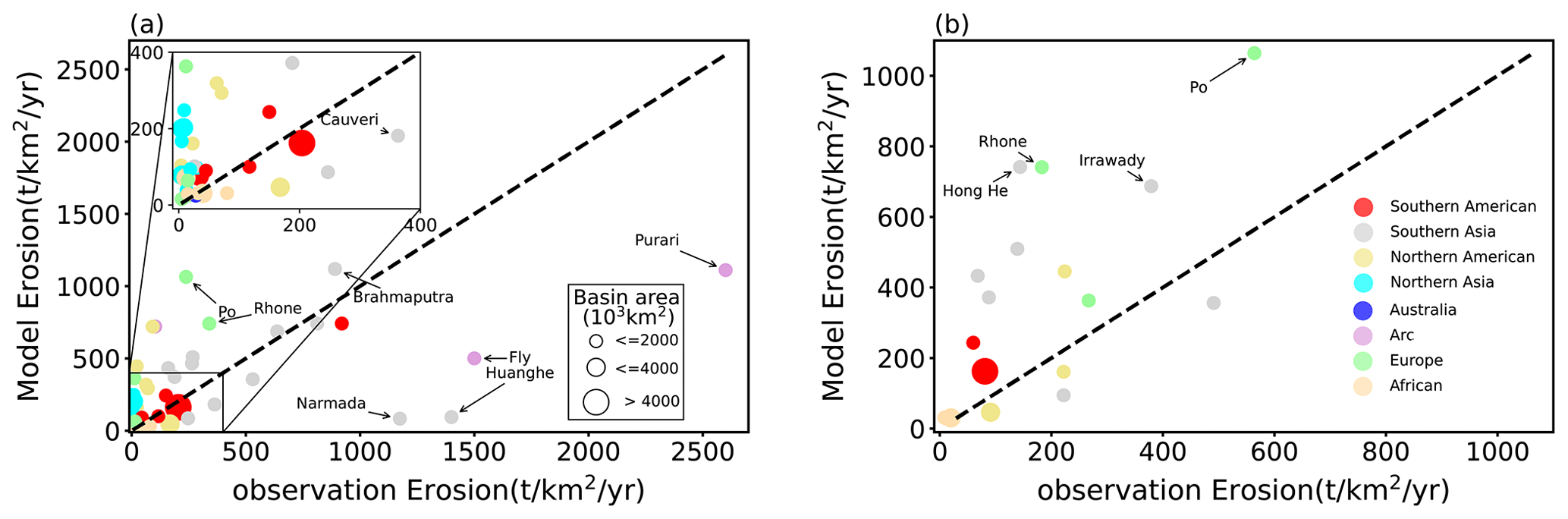
Figure 3 The comparison between model calculated and observed erosional fluxes for individual river basins. The Park20 model is used with the forcing data R_Yves and s1 (defined in Sect. 2.2). Different colors represent the regions where the basins are located, and the sizes represent the areas of the basins. In panel (a), the observed erosion rates are from TSS data (the last column in Table S3), and the observed erosion rates in panel (b) are from cosmogenic nuclide analysis, from which data are available for only 18 rivers (the penultimate column in Table S3).

2.2.6 Vegetation

The primary vegetation data used herein are the areal fraction of different vegetation types and their associated leaf area index (LAI) provided by NCAR (Fig. S6c–d), which are derived by integrating observed land information (Lawrence and Chase, 2007). To test the performance of simulated vegetation, we also downloaded the preindustrial vegetation data simulated by the Lund–Potsdam–Jena General Ecosystem Simulator (LPJ-GUESS) dynamic vegetation model and the HadCM3 climate model (Allen et al., 2020). In the 4×CO₂ experiment, the vegetation changed with climate and the data were downloaded from the CMIP6 home page, while the vegetation was assumed to be the same as in the present day except where the land was covered by ice sheets in the LGM experiment by M. Zhang et al. (2022).

2.2.7 Leached soil

The global soil distribution data are obtained from the Harmonized World Soil Database v1.2 (FAO/IIASA/ISRIC/ISSCAS/JRC, 2012), which is provided by the Food and Agriculture Organization of the United Nations. Following Hartmann et al. (2014), we selected six specific soil types as leached soil, i.e., Ferralsols, Acrisols, Nitisols, Lixisols, Histosols and Gleysols. Figure S6b represents the proportion of leached soil within each grid cell, as determined according to the selected soil types.

2.3 Evaluation of model performance

The model–data discrepancy in silicate weathering flux is often measured by r² (e.g., Park et al., 2020):

$$\begin{array}{}\text{(11)}& r_{\log }^{\mathrm{2}}=\mathrm{1}-{\displaystyle \frac{\sum ({\text{log}}_{\mathrm{10}}\left(M_i\right)-{\text{log}}_{\mathrm{10}}\left(O_i\right){)}^{\mathrm{2}}}{\sum ({\text{log}}_{\mathrm{10}}\left(O_i\right)-\overline{{\text{log}}_{\mathrm{10}}\left(O\right)}{)}^{\mathrm{2}}}},\end{array}$$

where M_i and O_i are the model calculated and observed values, respectively, and the summation is over the index i. Since we are concerned with the global flux F_w and the weathering–climate sensitivity, M_i and O_i represent the catchment-weathering flux for river i rather than the weathering flux per unit area of the ith river basin. In the equation above, a logarithmic operation is taken to the values first before calculating the difference: a subscript “log” is thus added to differentiate it from the r² calculated using the original values directly.

$$\begin{array}{}\text{(12)}& r^{\mathrm{2}}=\mathrm{1}-{\displaystyle \frac{\sum (\left(M_i\right)-\left(O_i\right){)}^{\mathrm{2}}}{\sum (\left(O_i\right)-\overline{\left(O\right)}{)}^{\mathrm{2}}}}\end{array}$$

Using $r_{\log }^{\mathrm{2}}$ has the advantage of giving relatively balanced weights to both the very small and very large values, which is important because the weathering fluxes over different river basins differ a lot (Table S2). Park20 obtained their model parameters in Eq. (9) by maximizing $r_{\log }^{\mathrm{2}}$. However, although there is a relatively small systematic bias in the logarithmic model–data errors (the data points distribute more symmetrically against the zero line in Fig. 1f), Fig. 1a–c show that there is an obvious systematic bias in the direct model–data errors. For similar magnitudes of the observational silicate weathering fluxes, the bias is much larger over the low-latitude regions (Fig. 1b) than over the high-latitude (Fig. 1a) regions. The bias in the direct errors in Fig. 1b will lead to an overestimation of the global weathering flux F_w (the global integral of W in Eq. 9) and may also be a misestimate of the weathering–climate sensitivity. Therefore, we argue that using the sum of $r_{\log }^{\mathrm{2}}$ and r² (denoted as “R2” hereafter) is better than using either of them as the criteria of model validation.

2.4 Experiments

In the first set of experiments, the original model of Park20 is tested for the influence of climate data and erosion rates from different sources or the same source but in different time periods. As described above, the temperature data come from two sources, ERA5 and CRU, and the data from ERA5 are organized into three different time periods; the runoff data come from five sources, ERA5, GRUN and UNH from Park20, UNH updated herein and Yves, where both the ERA5 and GRUN data are also organized into three different time periods. Slope data come from two sources: Scotese and Wright (2018) and Park20. The erosion rates are calculated in three different ways which all used Eq. (7), but the parameter B has different values: B=1, B tuned according to TSS data and B tuned according to both TSS data and the cosmogenic nuclide analysis. In the last case, the cosmogenic nuclide analysis supersedes TSS data if both of them are available for a basin. There are $\mathrm{4}\times \mathrm{9}\times \mathrm{2}\times \mathrm{3}=\mathrm{216}$ experiments in total, which are summarized in Table S4.

In the second set of experiments, we try to improve the Park20 model by considering the effect of additional processes. In each of these experiments, rather than adopting the values from Park20, all the unknown model parameters (Table S1) are optimized again. Based on the results of the first set of experiments, only T_CRU is used for temperature, and R_Park, R_Yves and R_GRUN2 are used for runoff. Erosion correction is not applied (i.e., B=1), and both slope data s1 and s2 are tested. We will first show that changing the validation criteria (maximizing R2 rather than $r_{\log }^{\mathrm{2}}$) is able to alleviate the systematic bias so that there is no overall overestimation, but the model–data discrepancy becomes even larger. In order to reduce this discrepancy, we try three different methods. The first method is to consider the influence of the seasonal cycle of temperature on the soil production rate, which will change the regolith thickness. The second and third methods consider the influence of leached soil and vegetation, respectively, on erosion rates. All three methods act to reduce the silicate weathering fluxes in the tropical region relative to those at the mid to high latitudes. All of these experiments are summarized in Table 1 below.

To consider the effect of vegetation, two different approaches have been tried, denoted by “m1” and “m2” in Table 1. m1 and m2 use the LAI of global vegetation from NCAR and simulated by the LPJ vegetation model, respectively. The global total erosional flux in m1 and m2 is reduced due to the shielding effect of vegetation. In order for the global total erosional flux to remain consistent with the observed value (20 Gt yr⁻¹ in Park20), the erosion rate at every grid point is scaled uniformly (by changing k_e in Eq. 7). For the sensitivity test, the LAI values of the global vegetation of the LGM (“m3”) and 4×CO₂ (“m4”) are used (see Sect. 2.2.2).

Table 1 Summary of the second set of experiments.

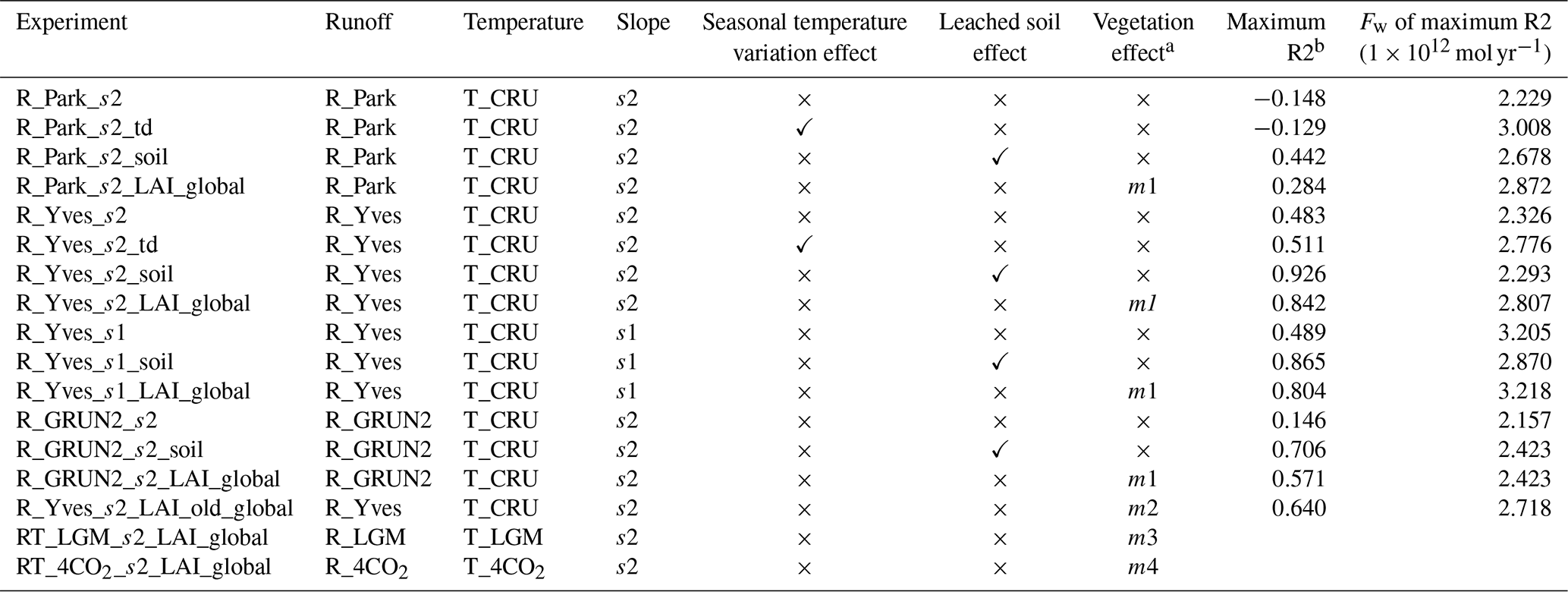
^a m1–m4: the global LAI is used and the global erosional flux is fixed to 20 Gt yr⁻¹ in all four cases, but the vegetation is from NCAR, the LPJ model, the LGM experiment and the 4×CO₂ experiment, respectively. ^b The maximum R2 here is obtained with observed silicate weathering fluxes from Gaillardet and HYBAM data together.

3 Results

We will first show whether the overestimated weathering fluxes over the tropical river basins of the Park20 model were due to the uncertainty in climate data or error in the calculated erosion rates. Then, we will re-estimate model parameters by balancing $r_{\log }^{\mathrm{2}}$ and r², i.e., by maximizing R2 defined in Sect. 2.3. After that, we propose and test a few different parameterizations to see whether they are effective in further decreasing the model–data discrepancy measured by R2 (Table 1). Without specific indications, all the results described below are for the present day.

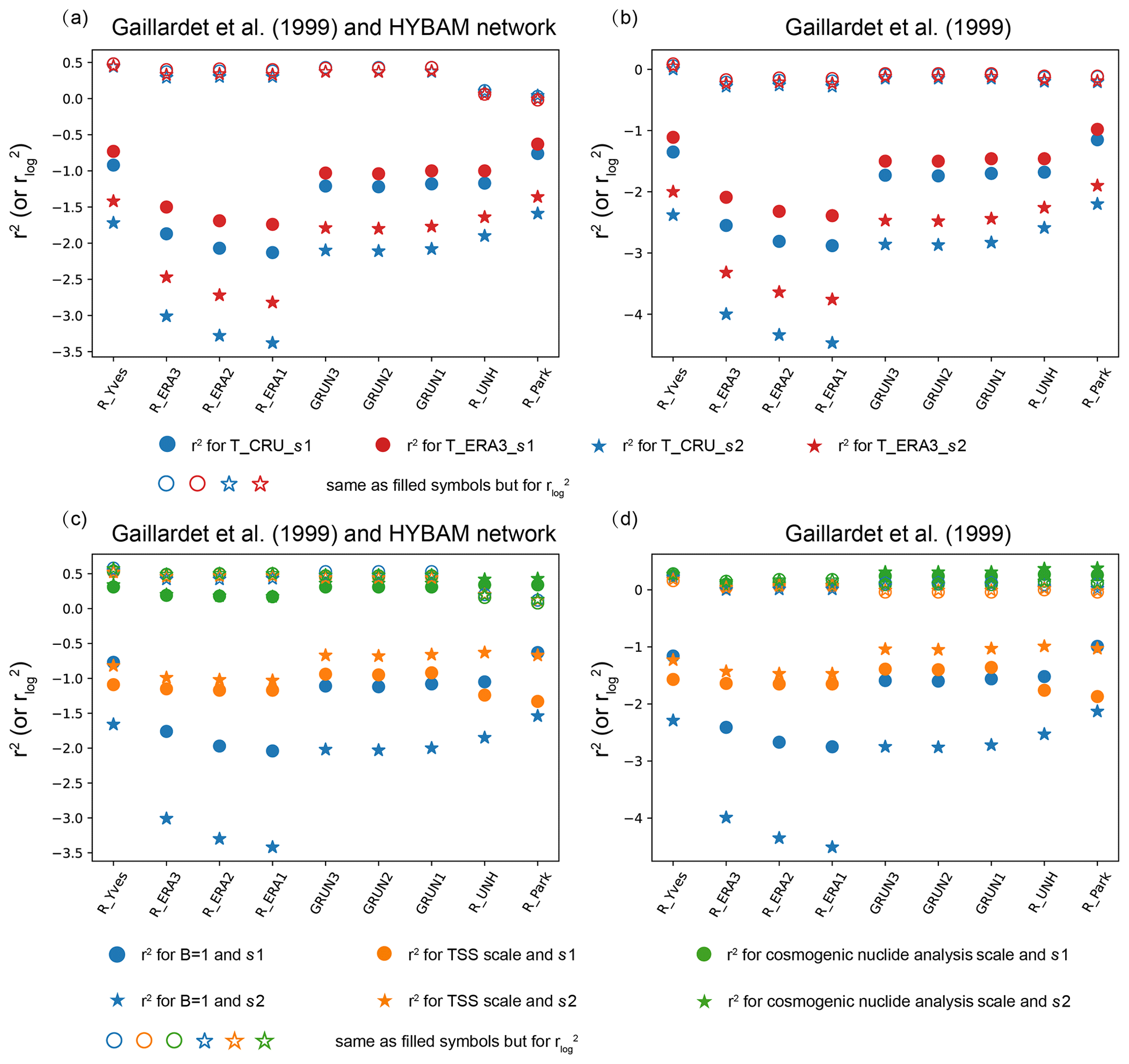
Figure 4 The r² (solid symbols) and $r_{\log }^{\mathrm{2}}$ (hollow symbols) calculated using different temperature, runoff and slope data. In panel (a), all the observed catchment-weathering fluxes in Park20 are used, while in panel (b) only the 51 basins of Gaillardet et al. (1999) are used to calculate r² and $r_{\log }^{\mathrm{2}}$. The runoff datasets are denoted on the x axis, and their names can be found in Fig. S3. Circles and pentagrams denote results calculated using slope data s1 and s2, respectively. Blue and red denote results calculated using the temperature data T_CRU and T_ERA3, respectively. The results using the temperature data T_ERA1 and T_ERA2 are very similar to that using T_ERA3 and thus are not shown. Panels (c) and (d) are similar to panels (a) and (b), except that here the temperature is fixed to T_CRU, while colors mean different ways of revising the erosion rate: no change (blue), the erosion rate of each basin scaled according to TSS data (orange) or cosmogenic nuclide analysis (green).

3.1 Influence of the climate forcing and erosion rate in the original Park20 model

For this series of tests, everything is the same as the Park20 model, except that the temperature, runoff and surface slope from different sources or different time periods are used. Results show that climate and slope data do have some impact on $r_{\log }^{\mathrm{2}}$ or r², especially the latter (Fig. 4a, b). The runoff data have the largest impact, followed by slope, and the temperature data have the least impact, probably because the uncertainties in temperature are small (Fig. S2). For runoff, the data from different centers give quite different r² values, while the data from the same center but different periods have a small effect. Although r² can vary from −0.5 to −4.47 in different cases, all of them are below zero (Fig. 4a, b), meaning a large model–data discrepancy. For all cases, overestimation in the weathering fluxes over tropical river basins persists (not shown but largely the same as shown in Fig. 1b), and the total global weathering flux is similarly overestimated.

If the observed erosion rates are used, r² is significantly improved, especially when the runoff datasets R_UNH and R_Park are used. The improvement is more significant when the erosion rates inferred from the cosmogenic nuclide analysis (Wittmann et al., 2020) are used. The tropical bias is also reduced but is still quite obvious (Figs. 5 and S7). Note that the results are improved even without tuning the empirical parameters in the Park20 model. This test shows us that the erosion rate may be a critical factor in alleviating the model bias. However, the erosion rates in either the past or the future are unknown and need to be parameterized if the model is to be applied to these time periods. Improving this parameterization is the major focus of our work herein and will be described in detail in what follows.

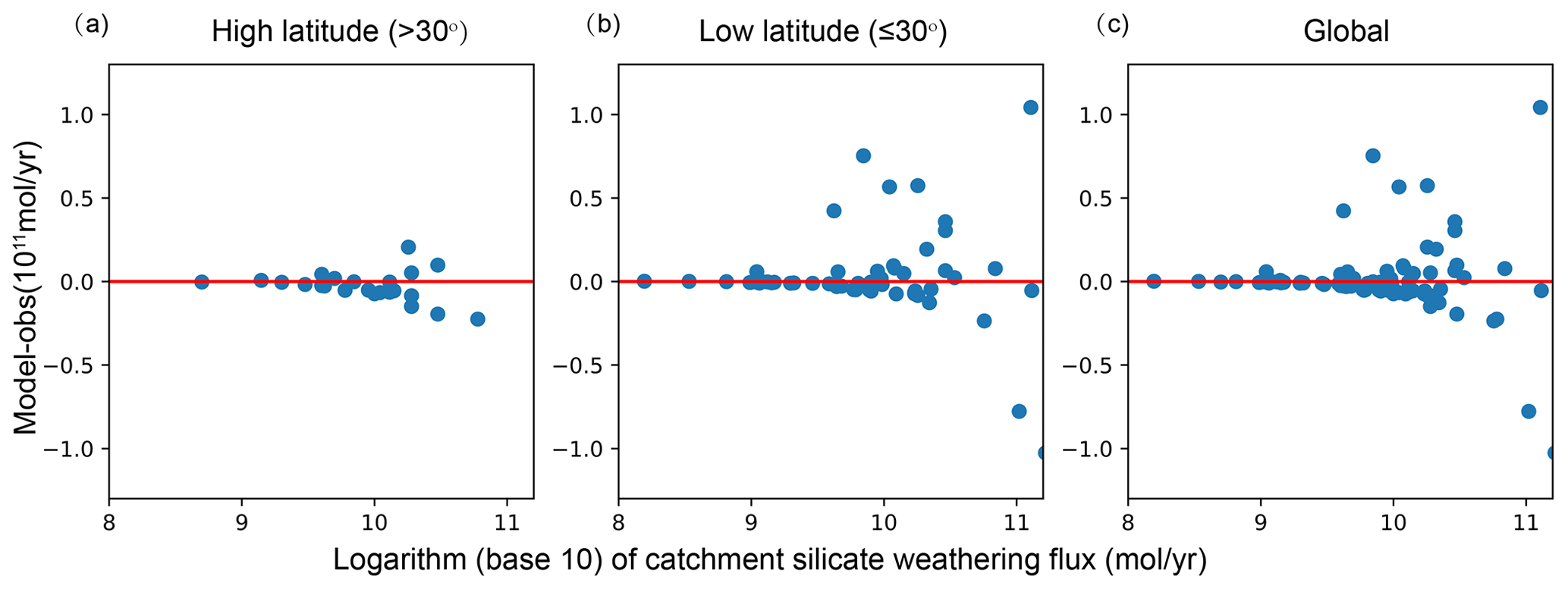
Figure 5 The difference (model − observation) in silicate weathering fluxes for 81 large rivers (more details can be found in Sect. 2.2.5). The model results are from the experiment T_CRU_R_Yves_s1_Be (Table S4), and the observation data are Gaillardet+HYBAM. The left, middle and right panels show rivers at the mid to high latitudes (if more than half of the river basin is located at or beyond 30° latitude), low latitudes (within 30° latitude) and over the whole globe, respectively. $r_{\log }^{\mathrm{2}}$ and r² are 0.54 and 0.31, respectively. The global total weathering flux is 3.95×10¹² mol yr⁻¹.

3.2 Maximizing R2 – a new control model

Other than the inaccuracy in the erosion rate (Fig. 3), the systematic bias in the Park20 model (Fig. 1) may also be due to the model parameters being searched by maximizing $r_{\log }^{\mathrm{2}}$. Here we check whether the bias can be alleviated by minimizing R2. Specifically, five parameters are searched with their searching ranges given in Table 2. Because the computational load of the model is relatively small, the searching is done by a forward calculation for all possible combinations. The total number of combinations is 240 240, and a full search takes 72 h on a desk computer and 1 h when 72 cores are used on a cluster. Only results for s2 are shown here, which aligns more closely with observations than those for s1 (not shown); results for s1 can be found in Table 1. Moreover, because of the relatively high sensitivity of the model results to runoff (Fig. 4), the model parameters are searched for three runoff datasets: R_Yves, R_Park and R_GRUN2. Only results for the former two are presented below, which is sufficient for demonstrating the effect of maximizing R2.

When calculating $r_{\log }^{\mathrm{2}}$ and r², two different sets of observed catchment-weathering fluxes have been used: Gailladet and Gailladet+HYBAM (see Sect. 2.2.5). The $r_{\log }^{\mathrm{2}}$, r² and R2 of all the parameter combinations are shown in Fig. 6, where each dot represents the result of a specific combination of model parameters and only the ones with values greater than 0 are shown. For Gailladet, the maximum $r_{\log }^{\mathrm{2}}$ and r² are −0.044 and 0.323, respectively, when R_Park is used (Fig. 6a; orange and light-blue dots, which represent $r_{\log }^{\mathrm{2}}$ and R2, respectively, do not show up because all their values are smaller than 0). For Gailladet+HYBAM, the maximum $r_{\log }^{\mathrm{2}}$ and r² become 0.138 and 0.349, respectively (Fig. 6b). It can be seen that F_w tends to be overestimated if $r_{\log }^{\mathrm{2}}$ is to be maximized ($F_{\mathrm{w}}=\mathrm{5.54}\times {\mathrm{10}}^{\mathrm{12}}$ mol yr⁻¹ at the peak of the orange dot group in Fig. 6b) but underestimated if r² is to be maximized ($F_{\mathrm{w}}=\mathrm{1.8}\times {\mathrm{10}}^{\mathrm{12}}$ mol yr⁻¹ at the peak of the purple-red dot group in Fig. 6b). Although the maximum $r_{\log }^{\mathrm{2}}$ (orange dots) and r² (purple-red dots) are both greater than 0 in Fig. 6b, no parameter combination can give relatively high $r_{\log }^{\mathrm{2}}$ and r² simultaneously, so that light-blue dots can appear. Using R_Yves improves $r_{\log }^{\mathrm{2}}$ significantly and thus R2; the maximum R2 value for Gailladet+HYBAM is 0.483 (Fig. 6d). It is notable that F_w is within the observational uncertainty range when R2 is maximized. The parameter combination associated with the maximum R2 is hence considered the new control model, and R_Yves is used in all the tests to be presented in what follows.

When R2 is maximized, either $r_{\log }^{\mathrm{2}}$ or r² or both are too small (Fig. 6). This means that errors for individual basins have increased overall, although the signs of errors are more balanced (Fig. 7) than before, so that the bias in F_w is small. However, inspection of the data points in Fig. 7 shows that the errors in the high-latitude region now have a negative bias compared to before (compare Figs. 7a and 1a), while the positive bias in the tropical region is somewhat reduced but remains (Fig. 7b). This redistribution of biases is clearly unsatisfying, and it may suggest that there is a missing process that distinguishes the tropical and extratropical regions.

Table 2 Model parameters and their values to be searched.

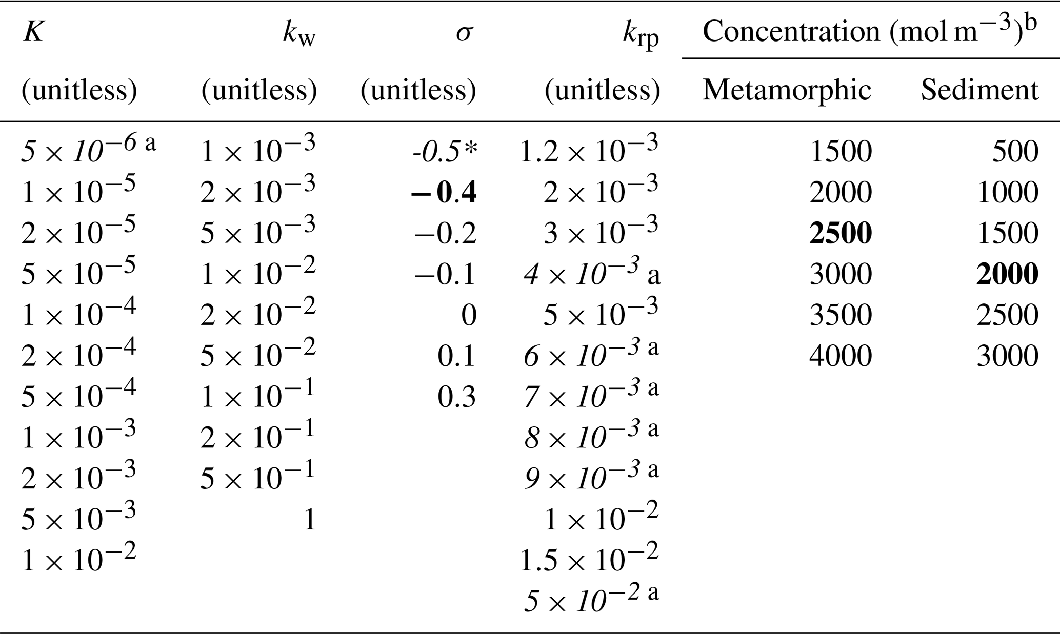
^a The data marked in italics are the additional values considered herein on top of those searched by Park20. The bold black values represent the optimal parameters selected by Park20. ^b Although the range of the cation concentration of metamorphic rocks overlaps with the sedimentary rocks, it is constrained so that the former must be larger than the latter during the search.

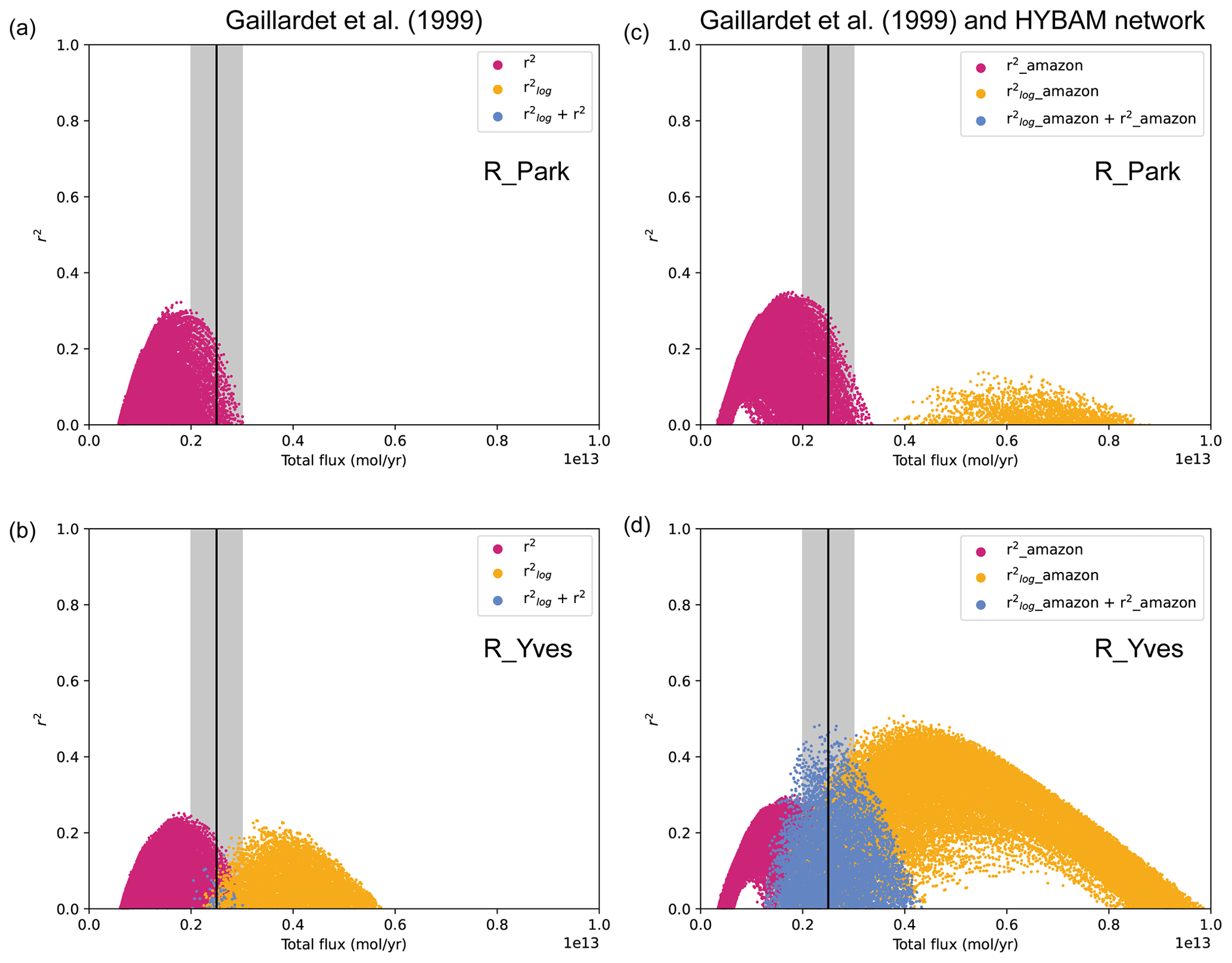
Figure 6 The $r_{\log }^{\mathrm{2}}$ (orange) and r² (purple-red) together with their sums (light blue) for all possible combinations of the parameters in Table 2. Only the cases with values greater than zero are shown. The results in panels (a), (b), (c) and (d), respectively, are for experiments R_park_s2 and R_ Yves_s2 defined in Table 1 and differ only in the runoff data used. The Gailladet and Gailladet+HYBAM are used as observational data in the left and right panels, respectively. The black vertical line and grey zone show the observed global total weathering flux (i.e., F_w) and its uncertainty range.

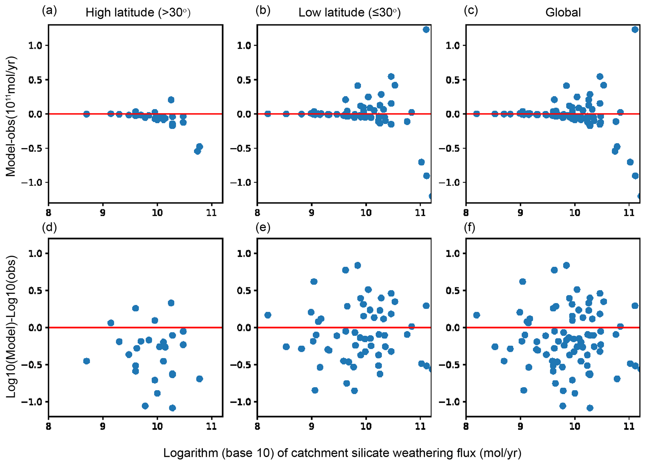
Figure 7 The difference (model − observation) in silicate weathering fluxes for 81 large rivers (more details can be found in Sect. 2.2.5). The model results are from the experiment R_Yves_s2 (Table S4), and the observation data are Gaillardet+HYBAM. The parameters are those that give the maximum R2 in Fig. 6d. The upper and lower panels show model-obs and log₁₀(model)-log₁₀(obs), respectively. The left (a, d), middle (b, e) and right (c, f) panels show rivers at the mid to high latitudes (if more than half of its river basin is located at or beyond 30° latitude), low latitudes (within 30° latitude) and over the whole globe, respectively. $r_{\log }^{\mathrm{2}}$ and r² are 0.33 and 0.16, respectively. The global total weathering flux F_w is 2.33×10¹² mol yr⁻¹.

3.3 Influence of the temperature-modulated soil production rate

Large seasonal changes in temperature can induce fractures in rocks and even form deep cracks in the surface soil layer (Liu et al., 2020), which may enhance the soil production rate at the base of the soil layer. Thus, the much weaker seasonal cycle in the tropical regions than at the higher latitudes (Fig. 6a) may be a factor to consider when calculating the erosion rate. To consider its influence, we assume that the soil production P_r is dependent on the amplitude of the seasonal cycle of surface temperature (defined as the difference between the maximum and minimum monthly temperatures), and the constant k_rp in Eq. (6) is now

$$\begin{array}{}\text{(13)}& k_{\mathrm{rp}}=\left({\displaystyle \frac{e^{(A_T-\mathrm{24})/c}-e^{-(A_T-\mathrm{24})/c}}{e^{(A_T-\mathrm{24})/c}+e^{-(A_T-\mathrm{24})/c}}}+b\right)\cdot a,\end{array}$$

where A_T is the amplitude of the seasonal cycle:

$$\begin{array}{}\text{(14)}& A_T=T_{\max }-T_{\min }\left(K\right).\end{array}$$

The constant 24 (K) in Eq. (13) is roughly the amplitude of the seasonal cycle at around 30° latitude (Fig. 8b). Across this critical amplitude, the soil production rate increases or decreases rapidly (Fig. 8a). Note that we have subjectively chosen to use a logistic function in Eq. (13) so as to make the soil production rate in the tropical region much lower than that in the extratropical region (Fig. 8b). This should be sufficient for the present purpose, which is to demonstrate whether the A_T could have any significant impact on silicate weathering. The values of a, b and c determine the minimum values of k_rp and its variation with latitude, and a total of 12 combinations of a, b and c are tested (Table S5, Fig. 8a).

The forward calculation is repeated to search the parameter combinations (Table 2) that maximize R2 for all combinations of a, b and c. Results show that the best $r_{\log }^{\mathrm{2}}$ and r² are obtained when a, b and c are equal to 0.0244, 1.05 and 8 (yellow dotted line in Fig. 8a), respectively, when only considering the observation data from Gaillardet and 0.015, 2.3 and 1 (red solid line in Fig. 8a), respectively, when including HYBAM data (Fig. 8c–d). Both $r_{\log }^{\mathrm{2}}$ and r² are improved in terms of the bias in F_w. Compared to the new control model in Sect. 3.2, F_w, corresponding to the peaks of both $r_{\log }^{\mathrm{2}}$ and r², is slightly closer to the observational value (compare Fig. 8c–d to Fig. 6c–d). However, the values of $r_{\log }^{\mathrm{2}}$ and r², corresponding to the highest R2, are 0.201 and 0.204 when the HYBAM data are not included, remaining small. When the HYBAM data are included for model evaluation, the R2 value is higher but no better than that of the new control model (compare Fig. 8d to Fig. 6d). Nevertheless, this model is superior to the new control model in that the biases in both the tropical and extratropical regions are reduced this time (not shown).

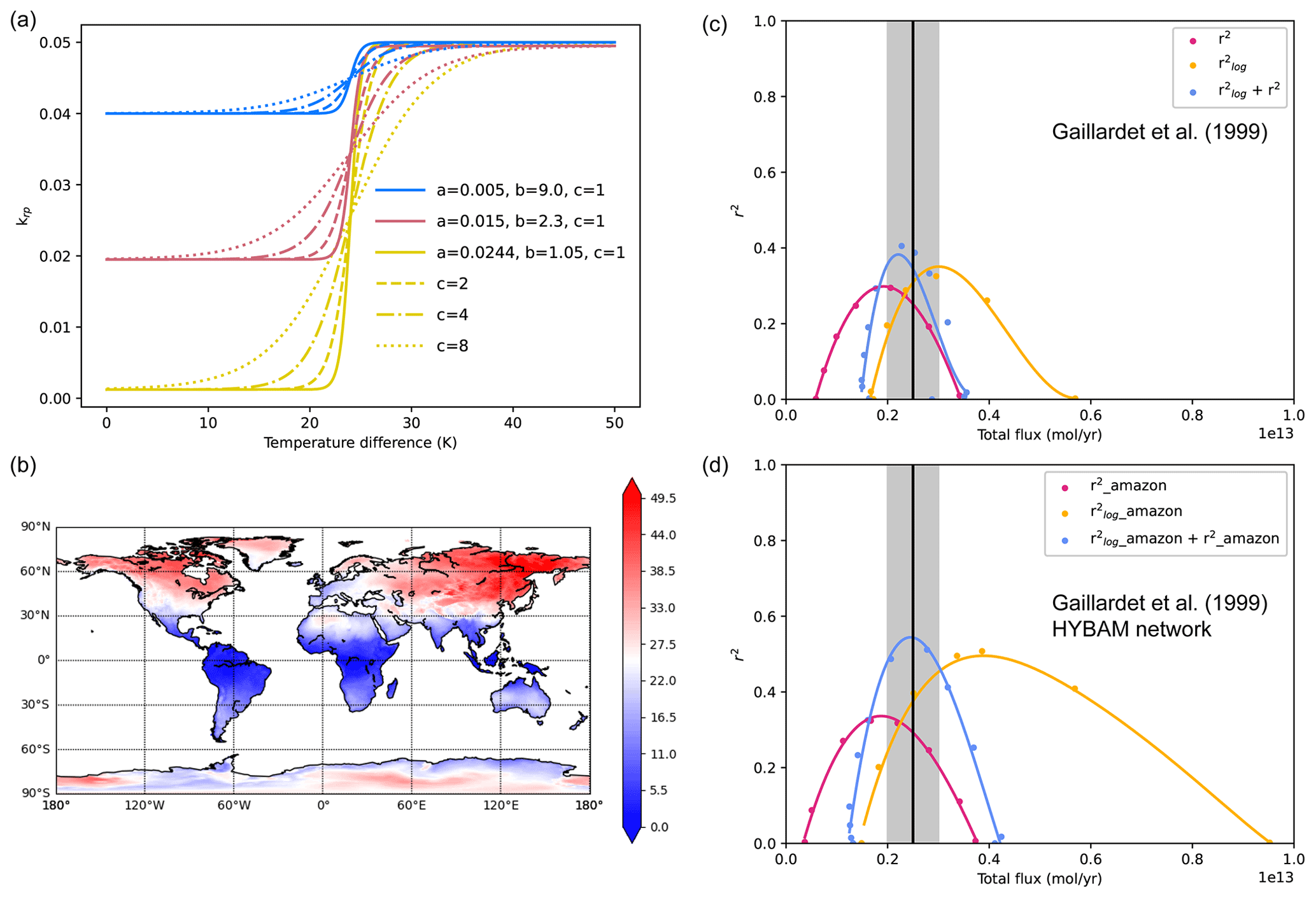
Figure 8 Possible effect of the seasonal cycle of surface temperature on the modeled silicate weathering flux. The soil production constant k_rp is assumed to depend on the amplitude of the seasonal cycle A_T (b) according to the functions in panel (a). Yellow, red and blue colors in panel (a) correspond to the three columns of Table S5, respectively. Parameter c in Eq. (14) has values of 8, 4 and 2 for the dotted, dash-dotted and dashed lines, respectively. Panel (c) shows the $r_{\log }^{\mathrm{2}}$ (orange), r² (purple-red) and R2 (light blue) of all possible combinations of the parameters with the effect of A_T considered. Instead of showing all the dots, only the envelopes (one for each color) are shown for the sake of clearness; the envelopes are obtained by curve fitting (cubic spline interpolation), and the data points used to do the fitting are still shown in the figure. Panel (d) is the same as panel (c), except that the HYBAM data are included in the observations. The results shown in panels (c) and (d) are from the experiment R_Yves_s2_td (Table 1). The black vertical line and grey zone show the observed F_w and its uncertainty range.

3.4 Implication of leached soil

Equation (9) tells us that local weathering flux is essentially the product of the erosion rate and the difference in the concentration of Ca and Mg cations between the bottom and top of the regolith. In the tropical regions, the cation concentration at the surface calculated by the Park20 model is near 0 where mountains are absent and is consistent with the distribution of leached soil (Figs. S6b and S8) defined in Sect. 2.2.7. The overestimation of tropical weathering fluxes (Fig. 1b) may thus indicate that the erosion rate in these regions is slower than that calculated by the model (Eq. 7). The cosmogenic nuclide analysis data do indicate lower erosion rates for the vast majority of rivers in the equatorial region than those from both TSS and the model calculation (Fig. 3b and Table S3). Figure 4 also shows that the results of the original Park20 model would be improved significantly if the observed erosion rates are used. Therefore, we think it is reasonable to slow down the erosion rate calculated by Eq. (7) when the areal fraction of leached soil in a grid box at mid to low latitudes (<30°) is greater than 20 %; the existence of such soil is an indication of slow erosion. The results are only slightly different if a different criterion is used because the areal fraction of leached soil is either very high or very low within the tropical region (Fig. S6b). Through a number of tests, it is found that the erosion rate by Eq. (7) should better be slowed down by an order of magnitude in these regions. The improvement of the erosion rate can be seen from Fig. 9b.

The model results are improved significantly with the simple change to the erosion rates above. The highest value of R2 reaches 0.73 and 0.93 when Gaillardet and Gaillardet+HYBAM, respectively, are used as observations (Fig. 10). Moreover, both $r_{\log }^{\mathrm{2}}$ and r² have high values (∼0.4) when R2 is at its maximum, higher than those obtained in Sect. 3.1 (Fig. 4c–d), where the model parameters were not optimized. Furthermore, the tropical bias is visibly reduced (compare Figs. 10 and 1b). These suggest that substantially slowing down the tropical erosion rates calculated by the Park20 model (Eq. 7) is an advisable choice. However, the appearance of leached soils is obviously a manifestation, not a reason, for the lower erosion rates. In addition, the distribution of leached soil is not available for the past or the future, just like the observed erosion rates tested in Sect. 3.1. Therefore, some other processes that are more fundamental and convenient than leached soil need to be found.

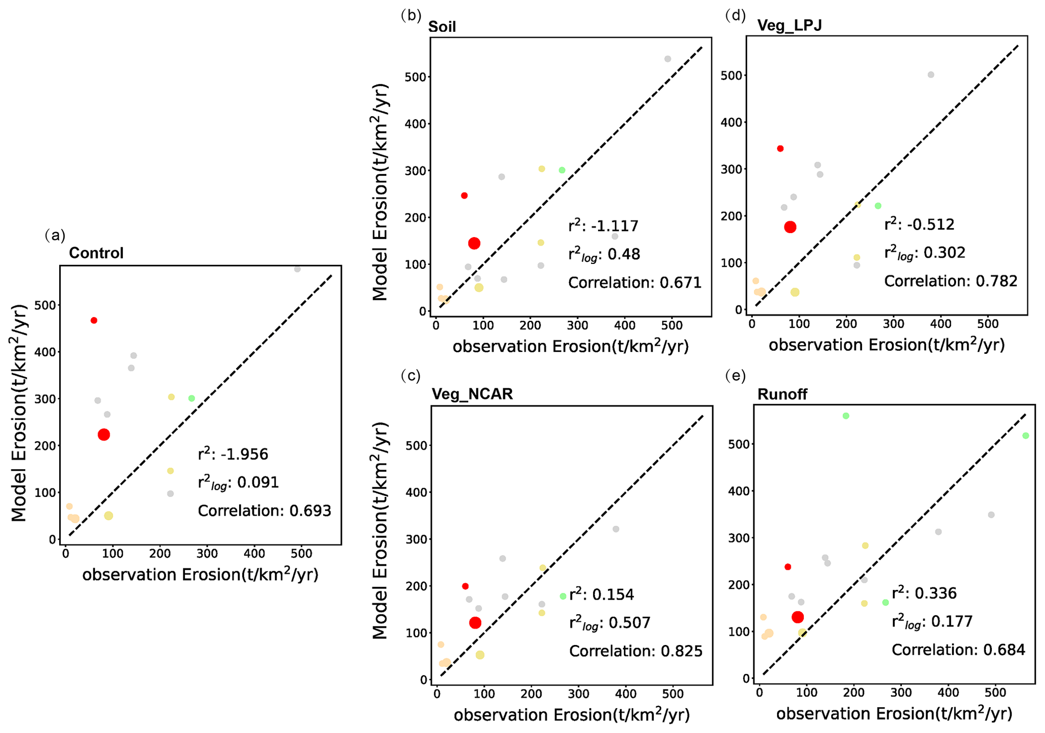
Figure 9 Comparison between modeled and observed erosion rates. The observed erosion rates are from the cosmogenic nuclide analysis of Wittmann et al. (2020). Some data points (different in each panel but definitely less than 4) do not show up because the axis limits are set to relatively smaller values for the sake of clarity (compare this to Fig. 3b), but $r_{\log }^{\mathrm{2}}$ and r² as well as the linear correlation are calculated using all 18 data points. Colors represent regions where the basins are located (see also Fig. 3b), and the sizes represent the area of the basins. Panels (a)–(e) differ in the way erosion is modeled. All the model calculations use R_Yves for runoff and s2 for the surface slope and use Eq. (7) with a different adjustment. (a) No adjustment. (b) The erosion rate is reduced by an order of magnitude where leached soils exist. (c) The erosion rate is reduced for a large LAI (from NCAR) according to Eq. (15). (d) Same as (c) except that the LAI is from the LPJ model. (e) Calculated by setting m in Eq. (7) to 0. In panels (c)–(e), all the values are rescaled uniformly so that the global total erosion is 20 Gt yr⁻¹.

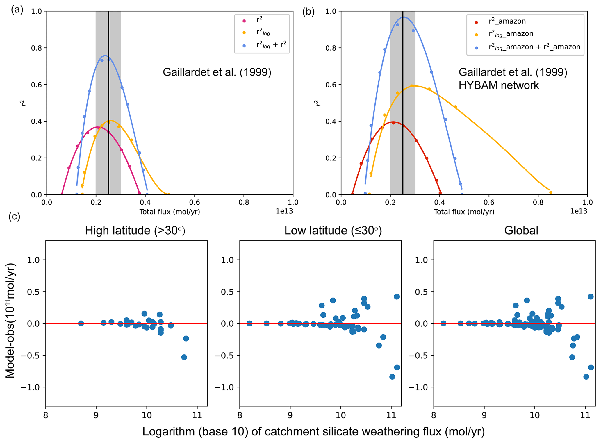
Figure 10 The effect of reduced erosion where leached soil is present in the modeled silicate weathering flux. Panels (a) and (b) show the $r_{\log }^{\mathrm{2}}$ (orange), r² (purple red) and R2 (light blue) of all possible combinations of the parameters. Similar to Fig. 8, only the envelopes and points used to fit the envelopes are shown. The results are from the experiment R_Yves_s2_soil (Table 1). The black vertical line and the grey zone show the observed F_w and its uncertainty range. Panel (c) shows the difference (model − observation) in silicate weathering fluxes for 81 large rivers, similar to Fig. 7a–c except that here the results corresponding to the highest R2 in panel (b) are shown. $r_{\log }^{\mathrm{2}}$ and r² are 0.56 and 0.37, respectively. The global total weathering flux is 2.29×10¹² mol yr⁻¹.

3.5 Influence of vegetation

It is observed that the distribution of leached soil (Fig. S6b) coincides with the flourishing of tropical vegetation (Fig. S6c, d) and may very well be a result of the latter. Although observations from arid regions indicate that the presence of vegetation significantly enhances mechanical erosion due to a rise in precipitation rates, mechanical erosion diminishes as vegetation cover increases in wet regions, owing to the dominant protective effects of vegetation (Mishra et al., 2019; Maffre et al., 2022). The presence of vegetation not only reduces the impact of raindrops on soil particles but also slows down the overland flow of water, decreasing the potential for soil detachment. Moreover, plant roots and organics contribute to soil cohesion and provide mechanical reinforcement (McMahon and Davies, 2018; Zeichner et al., 2021), thus reducing the overall likelihood of slope failures and landslides. Based on such thinking and the approximate coincidence between the distribution of leached soil and the region where the LAI is greater than 2, we design a way to modulate surface erosion with vegetation:

$$\begin{array}{}\text{(15)}& E=E\cdot \left(e^{-min\left(\mathrm{2},\text{LAI}\right)}\right).\end{array}$$

The basinal erosion rates calculated by the model in this way match those inferred from cosmogenic nuclide analysis better than when vegetation is not considered (Fig. 9c, d), substantiating the adjustment of erosion rate by vegetation. The erosion rates shown in Fig. 9c, d have been scaled up uniformly by changing k_e in order for the global total erosion flux to retain a value of 20 Gt yr⁻¹, although tests show that it only has a slight effect on the calculated silicate weathering fluxes. After considering the effect of vegetation, the maximum R2 can reach 0.84 (Fig. 11a, b), with the corresponding F_w being 2.8×10¹² mol yr⁻¹ (the experiment R_Yves_s2_LAI_global with the m1 method). Both $r_{\log }^{\mathrm{2}}$ and r² are also reasonably high (>0.3, Fig. S9a). Based on these results, here we propose that the suppression of erosion rates by vegetation was likely underestimated in previous studies on silicate weathering.

For the past or future, we will have to rely heavily on the model-simulated vegetation. However, the ability of current land models to simulate the vegetation and its response to climate change is still limited. Whether the effect of vegetation on silicate weathering can be properly considered is contingent upon how well the vegetation can be simulated. In one of the tests, the LAI simulated by the LPJ model (Fig. S10c, d; the experiment R_Yves_s2_LAI_old_global with the m2 method) was used. The results deteriorate substantially when the modeled global LAI was used; the maximum R2 merely attains a value of 0.64. This means that the defects in vegetation data cannot be compensated for by tuning other parameters in the weathering model. Therefore, getting better vegetation data by either reconstruction or model simulation is important for properly simulating silicate weathering of the past or future.

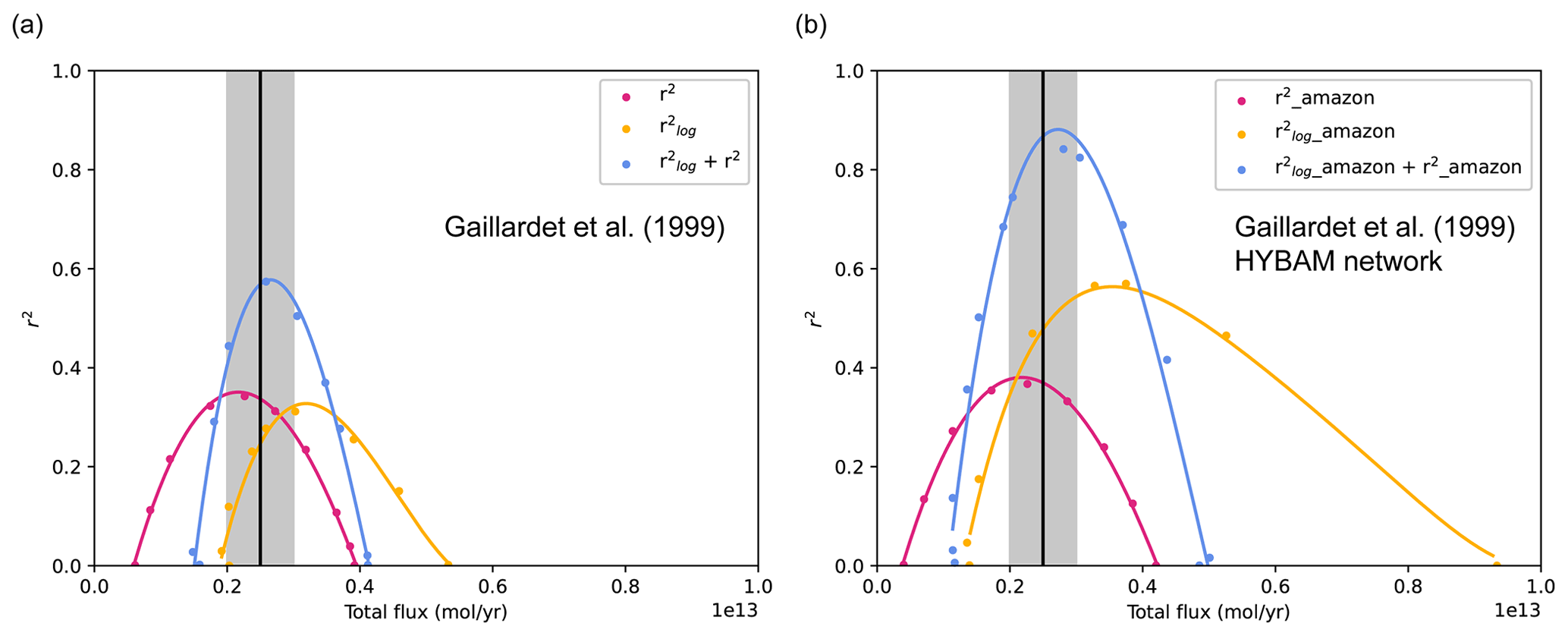
Figure 11 Panels (a) and (b) show the envelopes of $r_{\log }^{\mathrm{2}}$ (orange) and r² (purple red) and their sums (light blue) of all possible combinations of the parameters. The effect of vegetation is considered by using the global LAI, and the global total erosion rate is scaled to 20 Gt yr⁻¹. Only the cases with values greater than zero are shown. The black vertical line and the grey zone show the observed F_w and its uncertainty range. The results are from the experiment R_Yves_s2_LAI_global defined in Table 1.

3.6 Final parameters

A weathering model that adopts a parameterization for the effect of vegetation on erosion reduces the systematic error in the tropical region and is also easily applicable to other time periods. The F_w obtained by such a revised model is also closer to the most recently estimated global degassing flux (Müller et al., 2022). In this section, the optimal parameter set (that gives the highest R2) is provided for different combinations of runoff and surface slope (Table 3). The top five parameter sets with the highest R2 values (ranked based on the average R2 calculated for two sets of catchment-weathering flux measurements, R2^a and R2^b in Table 3) for each case are provided in Table 3. As can be seen, the parameter set highlighted in bold in Table 3 is amongst the best-performing parameter sets no matter which runoff or slope data are used. The weathering fluxes calculated using this set of parameters are much improved compared to those calculated using the original Park20 model in terms of both individual river basins (Fig. S11) and the global total (Fig. 11a, b). Subsequent calculations in this study are all based on this set of parameters unless otherwise stated.

Table 3 Parameters chosen in the case of the global LAI. Bold fonts represent the selected best-performing parameters among different slope or runoff data.

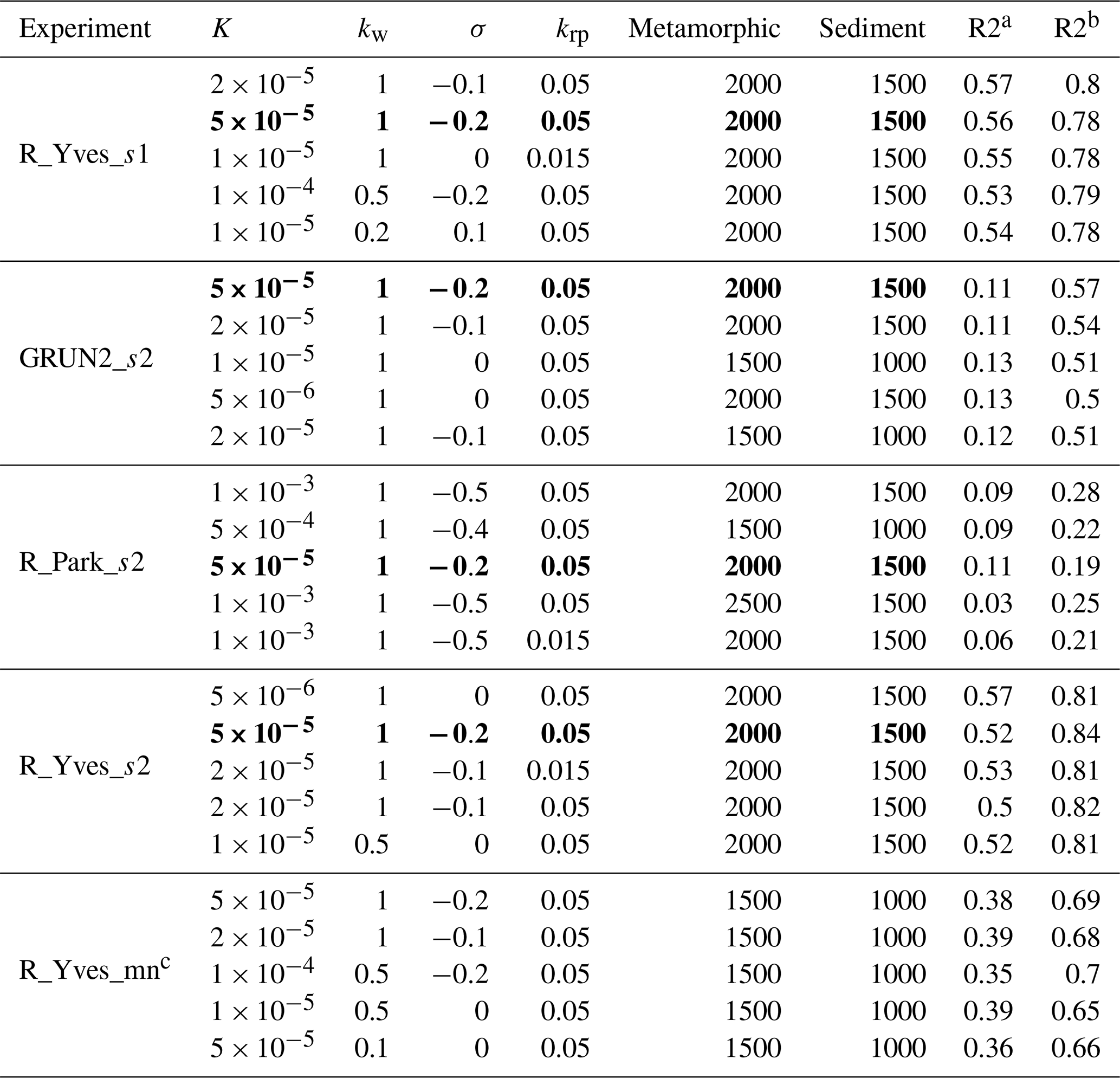
^a represents the fitting metrics with the observation of Gaillardet. ^b represents the observation data including the HYBAM network. ^c is the case that changes the erosion rate model by setting its sensitivity to the runoff to 0.

4 Discussion

4.1 Multiple effects of vegetation on silicate weathering

From the results presented in previous sections, we think that the silicate weathering fluxes calculated by previous models such as Park20 were systematically overestimated over the tropical region, and the overestimation was due at least in part to the overestimated erosion rate in this region. We thus propose that the overestimation in erosion was likely due to the underestimated effect of tropical vegetation on reducing erosion. The tests above show that this effect can be taken into account through a simple parameterization using the LAI, which can be obtained more easily by either reconstruction or model simulations (Binney et al., 2017; Krapp et al., 2021; Prentice et al., 2000; Prentice and Webb, 1998; Shao et al., 2018; Wang et al., 2008; Woillez et al., 2011; Yao et al., 2009; Andermann et al., 2022) for different time periods.

However, vegetation was generally thought to enhance silicate weathering by emitting organic acid (Caves Rugenstein et al., 2019; Berner, 2004, 1992), and the appearance of vegetation has been linked to the occurrence of a few ice ages in Earth's history (Lyla et al., 2011; Lenton et al., 2012). Here we are not arguing against such a mechanism and idea. Instead, we think that the ability of vegetation to enhance silicate weathering is universal and has been implicitly considered in model parameters such as the dissolution constant K in Eq. (2). In contrast, the effect of vegetation on soil protection could have been underestimated in silicate weathering models and could be geographically dependent. It is worth mentioning that Maffre et al. (2022) tested the effect of vegetation on slowing down soil erosion during the Devonian era, when vascular plants had just landed. Their work was more of a sensitivity study in that the observations (e.g., pCO₂) could not provide vigorous constraints, which the basinal weathering fluxes used here do.

4.2 Influence of runoff

Some studies propose that the influence of runoff might have been overestimated in existing erosion rate frameworks. For instance, in a renowned model for erosion, BQART, sensitivity to runoff was adjusted downward from 0.5 to 0.31 (Syvitski and Milliman, 2007). Consequently, we did a simple test by assuming no correlation between erosion rate and runoff, i.e., setting m in Eq. (7) to 0. As can be seen from Fig. 9e, the model–data discrepancy is also reduced quite significantly by this method. For weathering calculation, the maximum R2 value obtained under this assumption is approximately 0.718 (Fig. S10), achieving a smaller improvement compared to the vegetation parameterization above but a notable one compared to other methodologies. The optimal parameter sets obtained for this test are provided in Table 3. A not unreasonable conjecture is that removing the dependence of erosion on runoff implicitly takes into account part of the influence of vegetation, since vegetation and runoff generally exhibit a positive correlation under contemporary conditions (see Figs. S3 and S6c). Because the factors affecting vegetation include not just precipitation (highly related to runoff) but also temperature, sunlight and pCO₂, parameterizing erosion using vegetation is likely a superior way to using runoff.

4.3 Leached soil

It is worth emphasizing that the shielding effect on silicate weathering, although coincident with the distribution of leached soil, should be attributed to heavy vegetation as the former is likely a result of the retarding effect of the latter on erosion. This point can be partially inferred from the distribution of leached soils (Fig. 6b), LAI (Fig. 6c), surface slopes (Fig. S4a–b) and erosion rates (Fig. S4c–d). Leached soils should form in regions with relatively low erosion rates but no low silicate weathering rates. For example, regions with the lowest erosion rates are the desert regions where runoff is too small, but no leached soils form in these regions, probably due to the very low weathering rate. In some low-latitude regions where leached soils exist, the relatively low erosion rates (Fig. S4c–d) are consistent with the relatively small surface slope (i.e., flat terrain; Fig. S4a–b). However, in many other places (Fig. S6b), the erosion rates are relatively high (Fig. S4c–d) due to high runoff. These regions correspond more closely to the regions with a high LAI (Fig. 6c). Therefore, leached soils should be a result of a combination of vegetation development and relatively flat terrain, but the flat terrain is clearly not a necessary condition.

Godderis et al. (2008) also considered the effect of thick regolith cover on weathering by reducing the fluid that can reach the fresh bedrock, while we consider the effect herein by reducing the erosion rate. The two approaches agree with each other in that they both think that the weathering is transport-limited (i.e., fresh rocks are not exposed for weathering), but our approach is more direct and easier to apply to the paleo periods. This is because (1) the existence of the thick regolith cover is likely the result of weakened erosion (as described above) and (2) knowledge of regolith cover and thickness is unavailable for the past. Therefore, it seems better just to optimize the parameterization for the erosion rate directly, such as by considering the effect of land plants.

4.4 Sensitivity of global silicate weathering to climate change

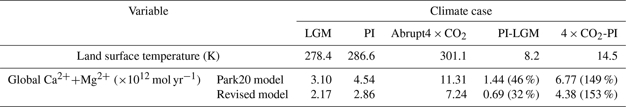
The climate data from the 4×CO₂ and LGM experiments (Sect. 2.2.2) are used to test the sensitivity of global silicate weathering to climate change. The land surface temperature increases from 278.4 K in the LGM to 286.6 K in the preindustrial and further to 301.1 K in the 4×CO₂ experiment. Note that these changes are highly dependent on the climate model used but do not matter for the purpose here, which is to demonstrate the sensitivity of silicate weathering to climate changes between the Park20 model and the revised model in Sect. 3.6.

According to the Park20 model, the global silicate weathering flux F_w increases by 1.44 (46 %) from the LGM to PI and by 6.77 (149 %) from PI to the 4×CO₂ situation (Table 4). For the revised model, F_w increases by 0.69 (32 %) from the LGM (experiment “RT_LGM_s2_LAI_global” with m3 in Table 1) to PI and by 4.38 (153 %) from PI to the 4×CO₂ situation (experiment “RT_4CO₂_s2_LAI_global” with m4 in Table 1). Thus, in terms of absolute values, the revised model is less sensitive to the climate, but in terms of relative values, the revised model is very similar to the original model. Because the relative change in the silicate weathering flux largely determines the relative change in pCO₂ (see Eq. 2 of Goddéris et al., 2023), which determines the climate change, the weathering–climate sensitivity of the revised model is similar to that of the original model. However, due to the fact that F_w and its variations (in terms of absolute values) in the revised model are much smaller than before, other processes such as the burial of organic carbon may have been more important in Earth's carbon cycle than thought before.

Note that, although the LGM and 4×CO₂ climates are used above to demonstrate the weathering–climate sensitivity, the timescales implied by these two experiments are only 10 000 and 100 years, respectively. These timescales are too short to be appropriate for the weathering models here, which assume that the weathering has reached a steady state; when the climate changes, vegetation may respond quickly (∼100 years), but the regolith layer and thus the weathering take a very long time to reach a new steady state.

Table 4 Sensitivity of global silicate weathering to climate.

4.5 Caveats and future directions

The previously used measure for model–data discrepancy is $r_{\log }^{\mathrm{2}}$, the maximization of which essentially optimizes the ratio between the model and the data. This measure has its advantages, but as we have shown above, such a measure cannot prevent the occurrence of a systematic error in the absolute difference between the model and the data (Fig. 1b). Optimizing r², on the other hand, tends to underestimate F_w. We thus propose optimizing the sum of $r_{\log }^{\mathrm{2}}$ and r² (i.e., R2) so that F_w is nearest to the observation. It turns out that simply maximizing R2, while largely removing the systematic bias, would give very low values for both $r_{\log }^{\mathrm{2}}$ and r² (Fig. 7), meaning that changing the measure for model–data discrepancy alone cannot improve the model. To resolve the problem, certain physical processes have to be rectified, e.g., by invoking the influence of vegetation on erosion. A relatively satisfactory fit was finally obtained. However, R2 is still a subjective choice which may not be ideal. For example, R2 measures the overall degree of dispersion of the model-calculated fluxes around the observed fluxes, but it does not measure the correlation in spatial patterns. This may be one way to improve the measure for model–data discrepancy in the future.

The erosion rates derived from cosmogenic nuclides, as compared to those obtained from TSS, significantly alleviate the issue of overestimation of tropical weathering fluxes calculated by the model (see Fig. 4c, d). This improvement is likely due to the fact that the erosion rates derived from the cosmogenic nuclide analysis represent the erosion for long timescales, whereas TSS may have been substantially contaminated by human activities such as land use and deforestation (Hewawasam et al., 2003). Additionally, TSS could have been eroded primarily from near the river mouth, overestimating the erosion, or substantial deposition may have occurred on the way, underestimating the erosion (Wittmann et al., 2020). The major problem with the cosmogenic nuclide data is that they only cover a limited number of river basins. Both datasets also have the problem that neither of them can provide the spatial distribution of erosion distribution within river basins. Given the large area of many of the river basins (Fig. 3; the size of the circle represents the area of the river basins), uneven distribution of erosion within the river basin could have a great influence on the modeled weathering flux. More detailed observations of erosion rates and the related mechanisms are clearly needed in the future.

Although it seems that a simple parameterization for reducing the erosion rate by vegetation (Eq. 15) works well in improving model–data comparison, it must be noted that this may not be the sole or best resolution. The influence of vegetation on erosion may also depend on the local environment, which we have refrained from delving into further, primarily due to the plethora of uncertainties and insufficient constraints. Future observational evidence will be required to offer support for better parameterization. Another process that may be considered is the horizontal transport and deposition of materials. The current model is a one-dimensional one in which the regolith or soil comes from the bottom only, while in reality the soils can be eroded away easily and transported to another location, changing the local profile of the cation concentration.

5 Summary

A silicate weathering model that explicitly considers the regolith profile based on the formulation of GM09 and Park20 is studied in detail. This model has more than five underdetermined parameters which need to be constrained by the observed weathering fluxes for multiple river basins or watersheds over the globe. In doing so, the model–data discrepancy was normally measured by $r_{\log }^{\mathrm{2}}$ (Eq. 11; larger values mean smaller discrepancies), and the parameter space was then searched to maximize $r_{\log }^{\mathrm{2}}$. This method focuses more on minimizing the relative error (or discrepancy) than the absolute error. We demonstrate that the parameters determined this way tend to systematically overestimate the weathering fluxes over the tropical region, which leads to a significant overestimation of the global total flux F_w (Fig. 1). In addition, we show that such a problem is not due to uncertainties in the climate and surface slope data. We thus propose using R2 = $r_{\log }^{\mathrm{2}}+r^{\mathrm{2}}$ as a new measure of model–data discrepancy, the maximization of which reduces both the relative and absolute errors in a more balanced way. By searching for the optimal parameters using this new measure, globally unbiased weathering fluxes are indeed obtained (Figs. 6 and 7c). However, the bias is removed by increasing the bias over the extratropical region (Fig. 7a) rather than by reducing the bias over the tropical region (Fig. 7b). Moreover, the model–data discrepancy is large; either $r_{\log }^{\mathrm{2}}$ or r² is small. Therefore, some other processes must be considered to reduce the bias over the tropical region and to reduce the model–data discrepancy.

The influence of the seasonal cycle of temperature on soil production is tested first based on the consideration that a stronger seasonal cycle can fracture and shatter rocks more easily. Little improvement can be achieved by such consideration (Fig. 8c, d). Next, the erosion rate is reduced in tropical regions where there are leached soils. It is found that the model–data discrepancy of silicate weathering fluxes is greatly reduced in this test (Fig. 10). Due to the fact that leached soil is the result, not the cause, of weakened erosion and the fact that the distribution of leached soil is almost coincident with that of forest, we propose that heavy vegetation is able to slow down erosion significantly. A simple parameterization is then put forward to consider the effect of vegetation on erosion by using the global LAI (Eq. 15). The LAI is used because it is relatively easy to obtain for other periods of Earth's history from Earth system model simulations. The Park20 model is revised to add this parameterization, and the model parameters are re-optimized using criterion R2 (Table 3). This revised model fits the observed weathering fluxes better than the original Park20 model (Fig. 11), and the modeled F_w is more consistent with both the observation and the most recently constructed global outgassing. Note that we are not against the idea of the evolution of land plants in Earth-enhanced silicate weathering: it is just that heavy vegetation could hinder silicate weathering by slowing down erosion over rainy regions. High precipitation and runoff in these regions would otherwise induce high erosion rates.

The revised model simulates a much smaller F_w than the original Park20 model. Correspondingly, the changes in F_w also become smaller under the same climate changes (Table 4), although the relative changes in F_w remain similar to the original model. If the revised model is reliable, it implies that the variations of other sinks of carbon such as organic carbon could have played a more important role than previously thought in the models. It will be interesting to see how the reconstruction of the Phanerozoic carbon cycle using models (e.g., Berner and Kothavala, 2001) will be impacted when the shielding effect of vegetation on silicate weathering as proposed herein is considered.