Systematic and objective evaluation of Earth system models: PCMDI Metrics Package (PMP) version 3

Systematic, routine, and comprehensive evaluation of Earth system models (ESMs) facilitates benchmarking improvement across model generations and identifying the strengths and weaknesses of different model configurations. By gauging the consistency between models and observations, this endeavor is becoming increasingly necessary to objectively synthesize the thousands of simulations contributed to the Coupled Model Intercomparison Project (CMIP) to date. The Program for Climate Model Diagnosis and Intercomparison (PCMDI) Metrics Package (PMP) is an open-source Python software package that provides quick-look objective comparisons of ESMs with one another and with observations. The comparisons include metrics of large- to global-scale climatologies, tropical inter-annual and intra-seasonal variability modes such as the El Niño–Southern Oscillation (ENSO) and Madden–Julian Oscillation (MJO), extratropical modes of variability, regional monsoons, cloud radiative feedbacks, and high-frequency characteristics of simulated precipitation, including its extremes. The PMP comparison results are produced using all model simulations contributed to CMIP6 and earlier CMIP phases. An important objective of the PMP is to document the performance of ESMs participating in the recent phases of CMIP, together with providing version-controlled information for all datasets, software packages, and analysis codes being used in the evaluation process. Among other purposes, this also enables modeling groups to assess performance changes during the ESM development cycle in the context of the error distribution of the multi-model ensemble. Quantitative model evaluation provided by the PMP can assist modelers in their development priorities. In this paper, we provide an overview of the PMP, including its latest capabilities, and discuss its future direction.

1 Introduction

Earth system models (ESMs) are key tools for projecting climate change and conducting research to enhance our understanding of the Earth system. With the advancements in computing power and the increasing importance of climate projections, there has been an exponential growth in the diversity of ESM simulations. During the 1990s, the Atmospheric Model Intercomparison Project (AMIP; Gates, 1992; Gates et al., 1999) was a centralizing activity within the modeling community which led to the creation of the Coupled Model Intercomparison Project (CMIP; Meehl et al., 1997, 2000, 2007; Covey et al., 2003; Taylor et al., 2012). Since 1989, the Program for Climate Model Diagnosis and Intercomparison (PCMDI) has worked closely with the World Climate Research Programme's (WCRP) Working Group on Coupled Modeling (WGCM) and Working Group on Numerical Experimentation (WGNE) to design and implement these projects (Potter et al., 2011). The most recent phase of CMIP (CMIP6; Eyring et al., 2016b) provides a set of well-defined experiments that most climate modeling centers perform and subsequently makes results available for a large and diverse community to analyze.

Evaluating ESMs is a complex endeavor, given the vast range of climate characteristics across space- and timescales. A necessary step involves quantifying the consistency between ESMs with available observations. Climate model performance metrics have been widely used to objectively and quantitatively gauge the agreement between observations and simulations to summarize model behavior with a wide range of climate characteristics. Simple examples include either the model bias or the pattern similarity (correlation) between an observed and simulated field (e.g., Taylor, 2001). With the rapid growth in the number, scale, and complexity of simulations, the metrics have been used more routinely, as exemplified by the Intergovernmental Panel on Climate Change (IPCC) Assessment Reports (e.g., Gates et al., 1995; McAvaney et al., 2001; Randall et al., 2007; Flato et al., 2014; Eyring et al., 2021). A few studies have been exclusively devoted to objective model performance assessment using summary statistics. Lambert and Boer (2001) evaluated the first set of CMIP models from CMIP1 using statistics for the large-scale mean climate. Gleckler et al. (2008) identified a variety of factors relevant to model metrics and demonstrated techniques to quantify the relative strengths and weaknesses of the simulated mean climate. Reichler and Kim (2008) attempted to gauge model improvements across the early phases of CMIP. The scope of objective model evaluation has greatly broadened beyond the mean state in recent years (e.g., Gleckler et al., 2016; Eyring et al., 2019), including attempts to establish performance metrics for a wide range of climate variability (e.g., Kim et al., 2009; Sperber et al., 2013; Ahn et al., 2017; Fasullo et al., 2020; Lee et al., 2021b; Planton et al., 2021) and extremes (e.g., Sillmann et al., 2013; Srivastava et al., 2020; Wehner et al., 2020, 2021). Guilyardi et al. (2009) and Reed et al. (2022) emphasized that metrics should be concise, interpretable, informative, and intuitive.

With the growth of data size and diversity of ESM simulations, there has been a pressing need for the research community to become more efficient and systematic in evaluating ESMs and documenting their performances. To respond to the need, PCMDI developed the PCMDI Metrics Package (PMP) and released its first version in 2015 (see “Code and data availability” section for all versions). A centralizing goal of the PMP then and now is to quantitatively synthesize results from the archive of CMIP simulations via performance metrics that help characterize the overall agreement between models and observations (Gleckler et al., 2016). For our purposes, “performance metrics” are typically (but not exclusively) well-established statistical measures that quantify the consistency between observed and simulated characteristics. Common examples include a domain average bias, a root mean square error (RMSE), a spatial pattern correlation, or others, typically selected depending on the application. Another goal of the PMP is to further diversify the suite of high-level performance tests that help characterize the simulated climate. The results provided by the PMP are frequently used to address two overarching and recurring questions: (1) what are the relative strengths and weaknesses between different models? (2) How are models improving with further development? Addressing the second question is often referred to as “benchmarking”, and this motivates an important emphasis of the effort described in this paper – striving to advance the documentation of all data and results of the PMP in an open and ultimately reproducible manner.

In parallel, the current progress towards systematic model evaluation remains dynamic, with evolving approaches and many independent paths being pursued. This has resulted in the development of diversified model evaluation software packages. Examples in addition to the PMP include the ESMValTool (Eyring et al., 2016a, 2019, 2020; Righi et al., 2020), the Model Diagnostics Task Force (MDTF)-Diagnostics package (Maloney et al., 2019; Neelin et al., 2023), the International Land Model Benchmarking (ILAMB) software system (Collier et al., 2018) that focuses on land surface and carbon cycle metrics, and the International Ocean Model Benchmarking (IOMB) software system (Fu et al., 2022) that focuses on surface and upper-ocean biogeochemical variables. Some tools have been developed with a more targeted focus on a specific subject area, such as the Climate Variability Diagnostics Package (CVDP) that diagnoses climate variability modes (Phillips et al., 2014; Fasullo et al., 2020) and the Analyzing Scales of Precipitation (ASoP) that focuses on analyzing precipitation scales across space and time (Klingaman et al., 2017; Martin et al., 2017; Ordonez et al., 2021). The regional climate community also has actively developed metrics packages such as the Regional Climate Model Evaluation System (RCMES; H. Lee et al., 2018). Separately, a few climate modeling centers have developed their own model evaluation packages to assist in their in-house ESM development, e.g., the E3SM Diags (Zhang et al., 2022). There also have been other efforts to enhance the usability of in situ and field campaign observations in ESM evaluations, such as Atmospheric Radiation Measurement (ARM) data-oriented metrics and diagnostics package Diag (ARM-DIAGS; Zhang et al., 2018, 2020) and Earth System Model Aerosol–Cloud Diagnostics (ESMAC Diags; Tang et al., 2022, 2023). While they all have their own scientific priorities and technical approaches, the uniqueness of the PMP is its focus on the objective characterization of the physical climate system as simulated by community models. An important prioritization of the PMP is to advance all aspects of its workflow in an open, transparent, and reproducible manner, which is critical for benchmarking. The PMP summary statistics characterizing CMIP simulations are version-controlled and made publicly available as a resource to the community.

In this paper, we describe the latest update of the PMP and its focus on providing a diverse suite of summary statistics that can be used to construct “quick-look” summaries of ESM performance from simulations made publicly available to the research community, notably CMIP. The rest of the paper is organized as follows. In Sect. 2, we provide a technical description of the PMP and its accompanying reference datasets. In Sect. 3, we describe various sets of simulation metrics that provide an increasingly comprehensive portrayal of physical processes across timescales ranging from hours to centuries. In Sect. 4, we introduce the usage of the PMP for model benchmarking. We discuss the future direction and the remaining challenges in Sect. 5 and conclude with a summary in Sect. 6. To assist the reader, the table in Appendix A summarizes the acronyms used in this paper.

2 Software package and data description

The PMP is a Python-based open-source software framework (https://github.com/PCMDI/pcmdi_metrics, last access: 8 May 2024) designed to objectively gauge the consistency between ESMs and available observations via well-established statistics such as those discussed in Sect. 3. The PMP has been mainly used for the evaluation of CMIP-participating models. A subset of CMIP experiments, those conducted using the observation forcings such as “Historical” and “AMIP” (Eyring et al., 2016b), is particularly well suited for comparing models with observations. The AMIP experiment protocol constrains the simulation with prescribed sea surface temperature (SST), and the Historical experiment is conducted using coupled model simulations driven by observed varying natural and anthropogenic forcings. Some of the metrics applicable to these experiments may also be relevant to others (e.g., multi-century coupled control runs called “PiControl” and idealized “4xCO2” simulations that are designed for estimating climate sensitivity).

The PMP has been applied to multiple generations of CMIP models in a quasi-operational fashion as new simulations are made available, new analysis methods are incorporated, or new observational data become accessible (e.g., Gleckler et al., 2016; Planton et al., 2021; Lee et al., 2021b; Ahn et al., 2022). Shortly after simulations from the most recent phase of the CMIP (i.e., CMIP6) became accessible, the PMP quick-look summaries were provided on the PCMDI's website (https://pcmdi.llnl.gov/metrics/, last access: 8 May 2024), offering a resource to scientists involved in CMIP or others interested in the evaluation of ESMs. To facilitate this, at PCMDI the PMP is technically linked to the Earth System Grid Federation (ESGF) that is the CMIP data delivery infrastructure (Williams et al., 2016).

The primary deliverable of the PMP is a collection of summary statistics. We strive to make the baseline results (raw statistics) publicly available and well-documented and continue to make advances with this objective as a priority. For our purposes, we are referring to model performance “summary statistics” and “metrics” interchangeably, although in some situations we consider there to be an important distinction. For us, a genuine performance metric constitutes a well-defined and established statistic that has been used in a very specific way (e.g., a particular variable, analysis, and domain) for long-term benchmarking (see Sect. 4). The distinction between summary statistics and metrics is application-dependent and evolving as the community advances efforts to establish quasi-operational capabilities to gauge ESM performance. Some visualization capabilities described in Sect. 3 are made available through the PMP. Users can also further explore the model–data comparisons using their preferred visualization methods or incorporate the results into their own studies from the summary statistics from the PMP. Noting the above, the scope of the PMP is fairly targeted. It is not intended to be “all-purpose”, e.g., by incorporating the vast range of diagnostics used in model evaluation.

The PMP is designed to readily work with model output that has been processed using the Climate Model Output Rewriter (CMOR; https://cmor.llnl.gov/, last access: 8 May 2024), which is a software library developed to prepare model output following the CF metadata conventions (Hassell et al., 2017; Eaton et al., 2022, http://cfconventions.org/, last access: 8 May 2024) in the Network Common Data Form (NetCDF). The CMOR is used by most modeling groups contributing to CMIP, ensuring all model output adheres to the CMIP data structures that themselves are based on the CF conventions. It is possible to use the PMP on model output that has not been prepared by CMOR, but this usually requires additional work, e.g., mapping the data to meet the community standards.

For reference datasets, the PMP uses observational products processed to be compliant with the Observations for Model Intercomparison Projects (obs4MIPs; https://pcmdi.github.io/obs4MIPs/, last access: 8 May 2024). The obs4MIPs effort was initiated circa 2010 (Gleckler et al., 2011) to advance the use of the observations in model evaluation and research. Substantial progress has been made in establishing obs4MIPs data standards that technically align with CMIP model output (e.g., Teixeira et al., 2014; Ferraro et al., 2015) with the data products published on the ESGF (Waliser et al., 2020). Obs4MIPs-compliant data were prepared with CMOR, and the data directly available via obs4MIPs are used as PMP reference datasets.

The PMP leverages other Python-based open-source tools and libraries such as xarray (Hoyer and Hamman, 2017), eofs (Dawson, 2016), and many others. One of the primary fundamental tools used in the latest PMP version is the Python package of Xarray Climate Data Analysis Tools (xCDAT; Vo et al., 2023; https://xcdat.readthedocs.io, last access: 8 May 2024). The xCDAT is developed to provide a more efficient, robust, and streamlined user experience in climate data analysis when using xarray (https://docs.xarray.dev/, last access: 8 May 2024). Portions of the PMP rely on the precursor of the xCDAT, a Python library called Community Data Analysis Tools (CDAT; Williams et al., 2009; Williams, 2014; Doutriaux et al., 2019), which has been fundamental since the early development stages of the PMP. The xarray software provides much of the functionality of CDAT (e.g., I/O, indexing, and subsetting). However, it lacks some key climate domain features that have been frequently used by scientists and exploited by the PMP (e.g., regridding and utilization of spatial/temporal bounds for computational operations) and which motivated the development of the xCDAT. Completing the transition from CDAT to xCDAT is a technical priority for the next version of the PMP.

To help advance open and reproducible science, the PMP has been maintained with an open-source policy with accompanying metadata for data reproducibility and reusability. The PMP code is distributed and released with version control. The installation process of the PMP is streamlined and user-friendly, leveraging the Anaconda distribution and the conda-forge channel. By employing conda and conda-forge, users benefit from a simplified and efficient installation experience, ensuring seamless integration of the PMP's functionality with minimal dependencies. This approach not only facilitates a straightforward deployment of the package but also enhances reproducibility and compatibility across different computing environments, thereby facilitating the accessibility and widespread adoption of the PMP within the scientific community. The pointer to the installation instructions can be found in the “Code and data availability” section. The PMP's online documentation (http://pcmdi.github.io/pcmdi_metrics/, last access: 8 May 2024) also includes installation instructions and a user demo for Jupyter Notebooks. A database of pre-calculated PMP statistics for all AMIP and Historical simulations in the CMIP archive are also available online. The archive of these statistics, stored as JSON files (Crockford, 2006; Crockford and Morningstar, 2017), includes versioning details for all codes and dependencies and data that were used for the calculations. These files provide the baseline results of the PMP (see the “Code and data availability” section for details). Advancements in model evaluation, along with the number of models and complexity of simulations, motivate more systematic documentation of performance summaries. With PMP workflow provenance information being recorded and the model and observational data standards maintained by PCMDI and colleagues, the PMP strives to make all its results reproducible.

3 Current PMP capabilities

The capabilities of the PMP have been expanded beyond its traditional large-scale performance summaries of the mean climate (Gleckler et al., 2008; Taylor, 2001). Various evaluation metrics have been implemented to the PMP for climate variability such as El Niño–Southern Oscillation (ENSO) (Planton et al., 2021; Lee et al., 2021a), extratropical modes of variability (Lee et al., 2019a, 2021b), intra-seasonal oscillation (Ahn et al., 2017), monsoons (Sperber and Annamalai, 2014), cloud feedback (Zelinka et al., 2022), and the characteristics of simulated precipitation (Pendergrass et al., 2020; Ahn et al., 2022, 2023) and extremes (Wehner et al., 2020, 2021). These PMP capabilities were built upon model performance tests that have resulted from research by PCMDI scientists and their collaborators. This section will provide an overview of each category of the current PMP evaluation metrics with their usage demonstrations.

3.1 Climatology

Mean state metrics quantify how well models simulate observed climatological fields at a large scale, gauged by a suite of well-established statistics such as RMSE, mean absolute error (MAE), and pattern correlation that have been used in climate research for decades. The focus is on the coupled Historical and atmospheric-only AMIP (Gates et al., 1999) simulations which are well-suited for comparison with observations. The PMP extracts seasonally and annually averaged fields of multiple variables from large-scale observationally based datasets and results from model simulations. Different obs4MIPs-compliant reference datasets are used, depending on the variable examined. When multiple reference datasets are available, one of them is considered a “default” (see Table 1) while others are identified as “alternatives”. The default datasets are typically state-of-the-art products, but in general, we lack definitive measures as to which is the most accurate, so the PMP metrics are routinely calculated with multiple products so that it can be determined what difference the selection of alternative observations makes to judgment made about model fidelity. The suite of mean climate metrics (all area-weighted) includes spatial and spatiotemporal RMSE, centered spatial RMSE, spatial mean bias, spatial standard deviation, spatial pattern correlation, and spatial and spatiotemporal MAE of the annual or seasonal climatological time mean (Gleckler et al., 2008). Often, a space–time statistic is used that gauges both the consistency of the observed and simulated climatological pattern and its seasonal evolution (see Eq. (1) in Gleckler et al., 2008). By default, results are available for selected large-scale domains, including “Global”, “Northern Hemisphere (NH) Extratropics” (30–90° N), “Tropics” (30° S–30° N), and “Southern Hemisphere (SH) Extratropics” (30–90° S). For each domain, results can also be computed for the land and ocean, land only, or ocean only. These commonly used domains highlight the application of the PMP mean climate statistics at large to global scales, but we note that the PMP allows users to define their own domains of interest, including at regional scales. Detailed instructions can be found on the PMP's online documentation (http://pcmdi.github.io/pcmdi_metrics, last access: 8 May 2024).

Table 1 List of variables and observation datasets used as reference datasets for the PMP's mean climate evaluation in this paper (Sect. 3.1 and Figs. 1–2). “As above” indicates the same as above.

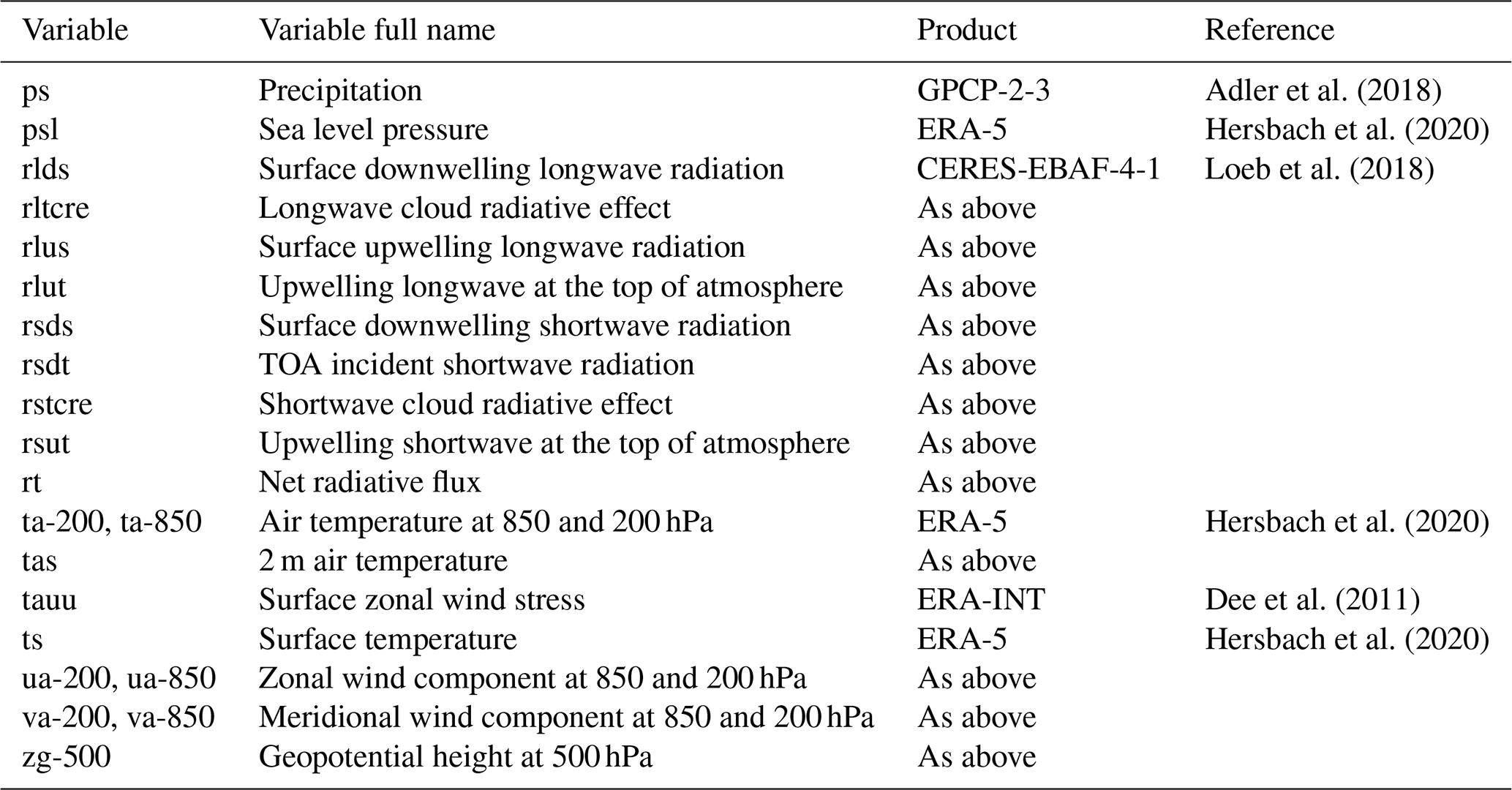
Although the primary deliverable of the PMP is the metrics, the PMP results can be visualized in various ways. For individual fields, we often first plot Taylor diagrams, a polar plot leveraging the relationship between the centered RMSE, the pattern correlation, and the observed and simulated standard deviation (Taylor, 2001). The Taylor diagram has become a standard plot in the model evaluation workflow across modeling centers and research communities (see Sect. 5). To interpret results across CMIP models for many variables, we routinely construct normalized portrait plots or Gleckler plots (Gleckler et al., 2008) that provide a quick-look examination of the strengths and weaknesses of different models. For example, in Fig. 1, the PMP results display quantitative information of simulated seasonal climatologies of various meteorological model variables via a normalized global spatial RMSE (Gleckler et al., 2008). Variants of this plot have been widely used for presenting model evaluation results, for example, in the IPCC Fifth (Flato et al., 2014; their Figs. 9.7, 9.12, and 9.37) and Sixth Assessment Reports (Eyring et al., 2021, Chap. 3; their Fig. 3.42). Because the error distribution across models is variable dependent, the statistics are often normalized to help reveal differences, in this case via the median RMSE across all models (see Gleckler et al., 2008, for more details). This normalization enables a common color scale to be used for all statistics on the portrait plot, highlighting the relative strengths and weaknesses of different models. In this example (Fig. 1), an error of −0.5 indicates that a model's error is 50 % smaller than the typical (median) error across all models, whereas an error of 0.5 is 50 % larger than the typical error in the multi-model ensemble. In many cases, the horizontal bands in the Gleckler plots show that simulations from a given modeling center have similar error structures relative to the multi-model ensemble.

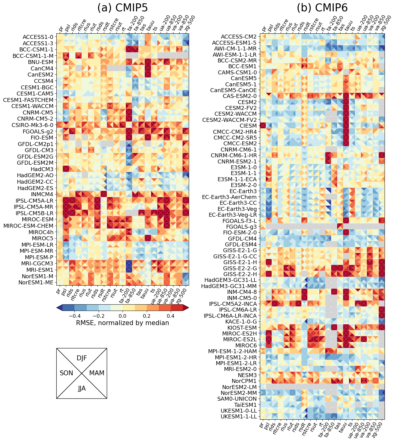
Figure 1 Portrait plot for spatial RMSE (uncentered) of global seasonal climatologies for (a) CMIP5 (models ACCESS1-0 to NorESM1-ME on the ordinate) and (b) CMIP6 (models ACCESS-CM2 to UKESM1-1-LL on the ordinate) for the 1981–2005 epoch. The RMSE is calculated for each season (shown as triangles in each box) over the globe, including both land and ocean, and model and reference data were interpolated to a common 2.5×2.5° grid. The RMSE of each variable is normalized by the median RMSE of all CMIP5 and CMIP6 models. A result of 0.2 (−0.2) is indicative of an error that is 20 % greater (lesser) than the median RMSE across all models. Models in each group are sorted in alphabetical order. Full names of variable names on the abscissa and their reference datasets can be found in Table 1. Detailed information for models can be found in the Earth System Documentation (ES-DOC, https://search.es-doc.org/, last access: 8 May 2024; Pascoe et al., 2020). The interactive version of the portrait plot in this figure is available on the PMP result pages on the PCMDI website (https://pcmdi.llnl.gov/metrics/mean_clim/, last access: 8 May 2024).

The parallel coordinate plot (Inselberg, 1997, 2008, 2016; Johansson and Forsell, 2016) that retains the absolute value of the error statistics is used to complement the portrait plot. Some previous studies have utilized parallel coordinate plots for analyzing climate model simulations (e.g., Steed et al., 2012; Wong et al., 2014; Wang et al., 2017), but to date, only a few studies have applied it to collective multi-ESM evaluations (see Fig. 7 in Boucher et al., 2020). In the PMP, we generally construct parallel coordinate plots using the same data as in a portrait plot. However, a fundamental difference is that metric values can be more easily scaled to highlight absolute values rather than the normalized relative results of the portrait plot. In this way, the portrait and parallel coordinate plots complement one another, and in some applications, it can be instructive to display both. Figure 2 shows the spatiotemporal RMSE, defined as the temporal average of spatial RMSE calculated in each month of the annual cycle, of CMIP5 and CMIP6 models in the format of parallel coordinate plot. Each vertical axis represents a different scalar measure gauging a distinct aspect of model fidelity. While polylines are frequently used to connect data points from the same source (i.e., metric values from the same model in our case) in parallel coordinate plots, we display results from each model using an identification symbol to reduce visual clutter in the plot and help identify outlier models. In the example of Fig. 2, each vertical axis is aligned with the median value midway through its max/min range scale. Thus, for each axis, the models in the lower half of the plot perform better than the CMIP5–CMIP6 multi-model median, while in the upper half, the opposite is true. For each vertical axis that is for a different model variable, we have added violin plots (Hintze and Nelson, 1998) to show probability density functions representing the distributions of model performance obtained from CMIP5 (shaded in blue on the left side of the axis) and CMIP6 (shaded in orange on the right side of the axis). Medians of each CMIP5 and CMIP6 group are highlighted using polylines, which indicates that the RMSE is reduced in CMIP6 relative to CMIP5 in general for the majority of the subset of model variables.

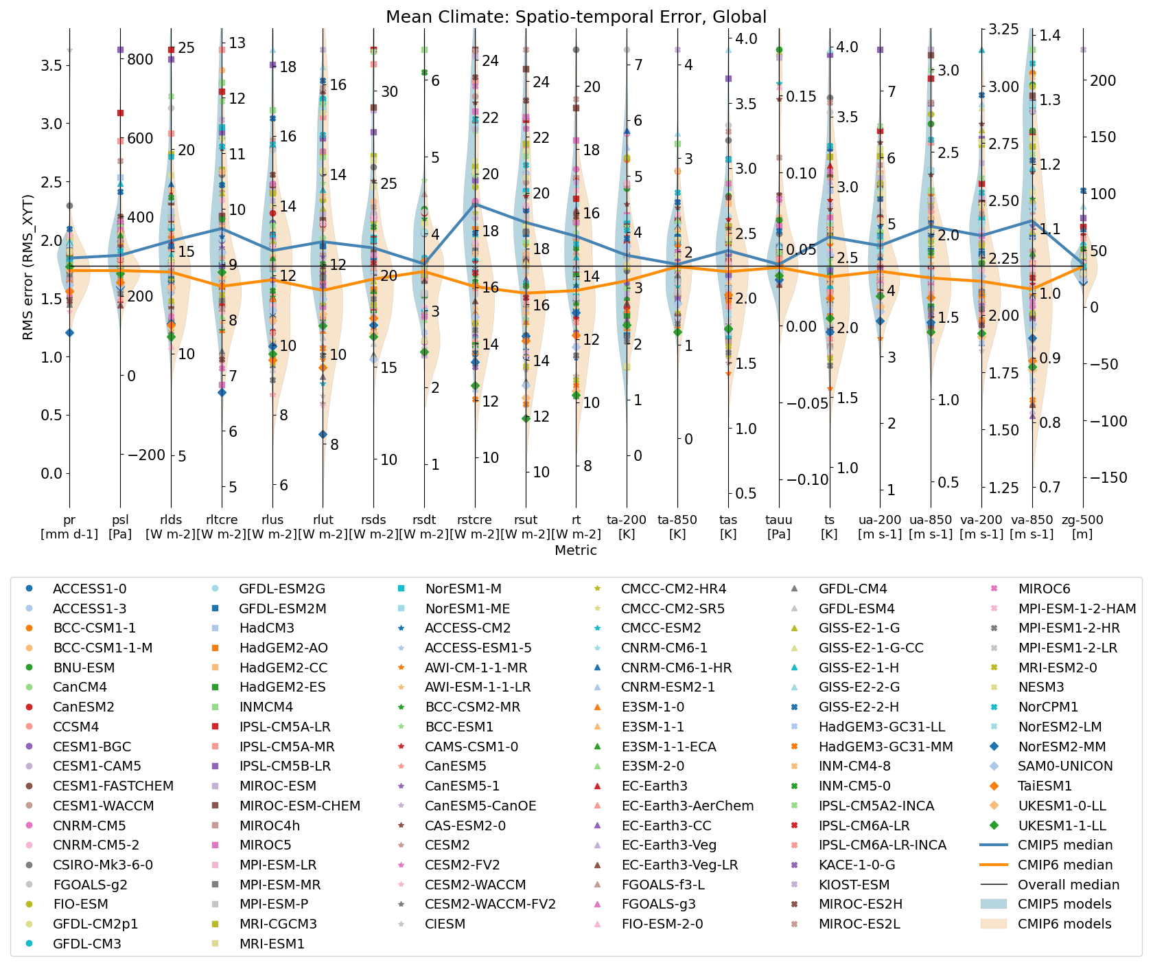
Figure 2 Parallel coordinate plot for spatiotemporal RMSE (Gleckler et al., 2008) from mean climate evaluation. Each vertical axis represents a different variable. Results from each model are displayed as symbols. The middle of each vertical axis is aligned with the median statistic of all CMIP5 and CMIP6 models. The cross-generation model distributions of model performance are shaded on the left (CMIP5; blue) and right (CMIP6; orange) sides of each axis. Also, medians from CMIP5 (blue) and CMIP6 (orange) model groups are highlighted as lines. Full names for model variables on the abscissa and their reference datasets can be found in Table 1. The time epoch used for this analysis is 1981–2005. Detailed information for models can be found in the Earth System Documentation (ES-DOC, https://search.es-doc.org/, last access: 8 May 2024; Pascoe et al., 2020). The interactive version of the portrait plot in this figure is available on the PMP result pages on the PCMDI website (https://pcmdi.llnl.gov/metrics/mean_clim/, last access: 8 May 2024).

3.2 El Niño–Southern Oscillation

The El Niño–Southern Oscillation (ENSO) is Earth's dominant inter-annual mode of climate variability, which impacts global climate via both regional oceanic effects and far-reaching atmospheric teleconnections (McPhaden et al., 2006, 2020). In response to increasing interest in a community approach to ENSO evaluation in models (Bellenger et al., 2014), the international Climate and Ocean Variability, Predictability and Change (CLIVAR) research focus on ENSO in a Changing Climate, together with the CLIVAR Pacific Region Panel, developed the CLIVAR ENSO Metrics Package (Planton et al., 2021) which is now utilized within the PMP. The ENSO metrics used to assess/evaluate the models are grouped into three categories: (1) performance (i.e., background climatology and basic ENSO characteristics), (2) teleconnections (ENSO's worldwide teleconnections), and (3) processes (ENSO's internal processes and feedback). Planton et al. (2021) found that CMIP6 models generally outperform CMIP5 models in several ENSO metrics, in particular for those related to tropical Pacific seasonal cycles and ENSO teleconnections. This effort is discussed in more detail in Planton et al. (2021), and detailed descriptions of each metric in the package are available in the ENSO package online open-source code repository on its GitHub wiki pages (see https://github.com/CLIVAR-PRP/ENSO_metrics/wiki, last access: 8 May 2024).

Figure 3 demonstrates the application of the ENSO metrics to CMIP6, showing the magnitudes of inter-model and inter-ensemble spreads, along with observational uncertainty varying across metrics. For a majority of the ENSO performance metrics, model error and inter-model spread are substantially larger than observational uncertainty (Fig. 3a–n). This highlights the systematic biases, like the double Intertropical Convergence Zone (ITCZ) (Fig. 3a), that are persisting through CMIP phases (Tian and Dong, 2020). Similarly, ENSO process metrics (Fig. 3t–w) indicate large errors in the feedback loops generating SST anomalies, indicating a different balance of processes in the model and in the reference and possibly compensating errors (Bayr et al., 2019; Guilyardi et al., 2020). In contrast, for ENSO teleconnection metrics, the observational uncertainty is substantially larger, thus challenging validation of model error (Fig. 3o–r). For some metrics, such as the ENSO duration (Fig. 3f), the ENSO asymmetry metric (Fig. 3i), and the ocean-driven SST metric (Fig. 3s), there are larger inter-ensemble spreads than the inter-model spreads. From such results, Lee et al. (2021a) examined the inter-model and inter-member spread of these metrics from the large ensembles available from CMIP6 and the U.S. CLIVAR Large Ensemble Working Group. They argued that to robustly characterize baseline ENSO characteristics and physical processes, larger ensemble sizes are needed compared to existing state-of-the-art ensemble projects. By applying the ENSO metrics to historical and PiControl simulations of CMIP6 via the PMP, Planton et al. (2023) developed equations based on statistical theory to estimate the required ensemble size for a user-defined uncertainty range.

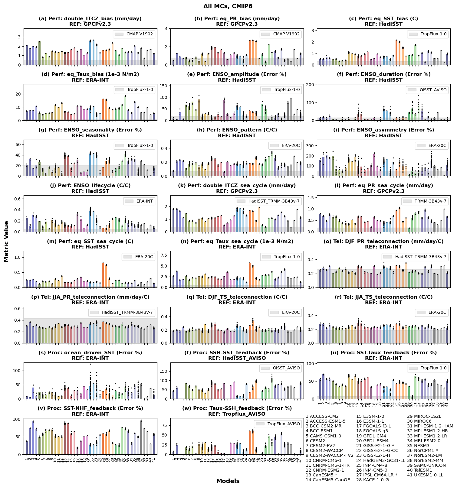
Figure 3 Application of ENSO metrics to CMIP6 models. Model names with an asterisk (^*) indicate that 10 or more ensemble members were used in this analysis. Dots indicate metric values from individual ensemble members, while bars indicate the average of metric values across the ensemble members. Bars colored for easier identification of model names at the bottom of the figure. Metrics were grouped into three metrics collections: (a–n) ENSO performance, (o–r) ENSO teleconnections, and (s–w) ENSO processes. The names of individual metrics and default reference datasets being used are noted on top of each panel, and the observational uncertainty by applying the metrics for alternative reference datasets noted on the upper right of each panel is shown as gray shaded. Detailed descriptions for each metric can be found at https://github.com/CLIVAR-PRP/ENSO_metrics/wiki (last access: 8 May 2024).

3.3 Extratropical modes of variability

The PMP includes objective measures of the pattern and amplitude of extratropical modes of variability from PCMDI's research, which has expanded beyond its traditional large-scale performance summaries to include inter-annual variability, considering increasing interest in setting an objective approach for the collective evaluation of multiple modes. Extratropical modes of variability (ETMoV) metrics in the PMP were developed by Lee et al. (2019a) that stem from earlier works (e.g., Stoner et al., 2009; Phillips et al., 2014). Lee et al. (2019a) illustrated a challenge when evaluating modes of variability using the traditional empirical orthogonal functions (EOF). In particular, when a higher-order EOF of a model more closely corresponds to a lower-order observationally based EOF (or vice versa), it can significantly affect conclusions drawn about model performance. To circumvent this issue in evaluating the inter-annual variability modes, Lee et al. (2019a) used the common basis function (CBF) approach that projects the observed EOF pattern onto model anomalies. This approach has been previously applied for the evaluation of intra-seasonal variability modes (Sperber, 2004; Sperber et al., 2005). In the PMP, the CBF approach is taken as a default method, and the traditional EOF approach is also enabled as an option for the ETMoV metrics calculations.

The ETMoV metrics in the PMP measure simulated patterns and amplitudes of ETMoV and quantify their agreement with observations (e.g., Lee et al., 2019a, 2021b). The PMP's ETMoV metrics evaluate five atmospheric modes – the Northern Annular Mode (NAM), North Atlantic Oscillation (NAO), Pacific North America pattern (PNA), North Pacific Oscillation (NPO), and Southern Annular Mode (SAM) – and three ocean modes diagnosed by the variance of sea surface temperature – Pacific Decadal Oscillation (PDO), North Pacific Gyre Oscillation (NPGO), and Atlantic Multi-decadal Oscillation (AMO). The AMO is included for experimental purposes, considering the significant uncertainty in detecting the AMO (Deser and Philips, 2021; Zhao et al., 2022). The amplitude metric, defined as the ratio of standard deviations of the model and observed principal components, has been used to examine the evolution of the performance of models across different CMIP generations (Fig. 4). Green shading predominates, indicating where the simulated amplitude of variability is similar to observations. In some cases, such as for SAM in September–October–November (SON), the models overestimate the observed amplitude.

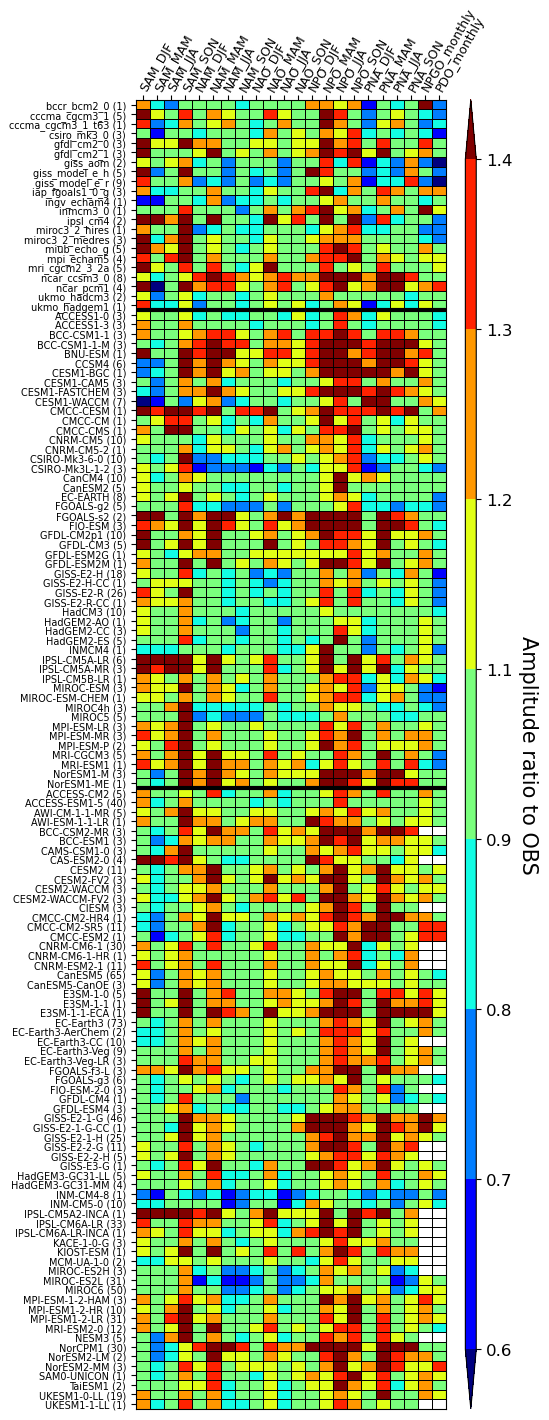
Figure 4 Portrait plots of the amplitude of extratropical modes of variability simulated by CMIP3, CMIP5, and CMIP6 models in their historical or equivalent simulations, as gauged by the ratio of spatiotemporal standard deviations of the model and observed principal components (PCs), obtained using the CBF method in the PMP. Columns (horizontal axis) are for mode and season, and rows (vertical axis) are for models from CMIP3 (top), CMIP5 (middle), and CMIP6 (bottom), separated by horizontal thick black lines. For sea-level-pressure-based modes (SAM, NAM, NAO, NPO, and PNA) in the upper-left hand triangle, the model results are shown relative to NOAA-20CR. For SST-based modes (NPGO and PDO), results are shown relative to HadISSTv1.1. Numbers in parentheses following model names indicate the number of ensemble members for the model. Metrics for individual ensemble members were averaged for each model. White boxes indicate a missing value.

The PMP's ETMoV metrics have been used in several model evaluation studies. For example, Orbe et al. (2020) analyzed models from US climate modeling groups, including the U.S. Department of Energy (DOE), National Aeronautics and Space Administration (NASA), National Center for Atmospheric Research (NCAR), and National Oceanic and Atmospheric Administration (NOAA), where they found that the improvement in the ETMoV performance is highly dependent on the mode and season when comparing across different generations of those models. Sung et al. (2021) examined the performance of models run at the Korea Meteorological Administration (K-ACE and UKESM1) in reproducing ETMoVs from their Historical simulations and concluded that these models reasonably capture most ETMoVs. Lee et al. (2021b) collectively evaluated ∼ 130 models from CMIP3, CMIP5, and CMIP6 archive databases using their ∼ 850 Historical and ∼ 300 AMIP simulations, where they found the spatial pattern skill improved in CMIP6 compared to CMIP5 or CMIP3 for most modes and seasons, while the improvement in amplitude skill is not clear. Arcodia et al. (2023) used the PMP to derive PDO and AMO to investigate their role in decadal variability in the subseasonal predictability of precipitation over the western coast of North America and concluded that no significant relationship was found.

3.4 Intra-seasonal oscillation

The PMP has implemented metrics for the Madden–Julian Oscillation (MJO; Madden and Julian, 1971, 1972, 1994). The MJO is the dominant mode of tropical intra-seasonal variability characterized by a pronounced eastward propagation of large-scale atmospheric circulation coupled with convection, with a typical periodicity of 30–60 d. Selected metrics from the MJO diagnostics package, developed by the CLIVAR MJO Working Group (Waliser et al., 2009), have been implemented in the PMP, following Ahn et al. (2017).

We have particularly focused on metrics for the MJO propagation: east : west power ratio (EWR) and east power normalized by observation (EOR). The EWR is proposed by Zhang and Hendon (1997), which is defined as the ratio of the total spectral power over the MJO band (eastward propagating, wavenumbers 1–3, and period of 30–60 d) to that of its westward-propagating counterpart in the wavenumber frequency power spectra. The EWR metric has been widely used in the community to examine the robustness of the eastward-propagating feature of the MJO (e.g., Hendon et al., 1999; Lin et al., 2006; Kim et al., 2009; Ahn et al., 2017). The EOR is formulated by normalizing a model's spectral power within the MJO band by the corresponding observed value. Ahn et al. (2017) showed EWRs and EORs of the CMIP5 models. Using daily precipitation, the PMP calculates EWR and EOR separately for boreal winter (November to April) and boreal summer (March to October). We apply the frequency–wavenumber decomposition method to precipitation from observations (Global Precipitation Climatology Project (GPCP)-based; 1997–2010) and the CMIP5 and CMIP6 Historical simulations for 1985–2004. For disturbances with wavenumbers 1–3 and frequencies corresponding to 30–60 d, it is clear in observations that the eastward-propagating signal dominates over its westward-propagating counterpart with an EWR value of about 2.49 (Fig. 5a). Figure 5b shows the wavenumber–frequency power spectrum from CMIP5 IPSL-CM5B-LR as an example, which has an EWR value that is comparable to the observed value.

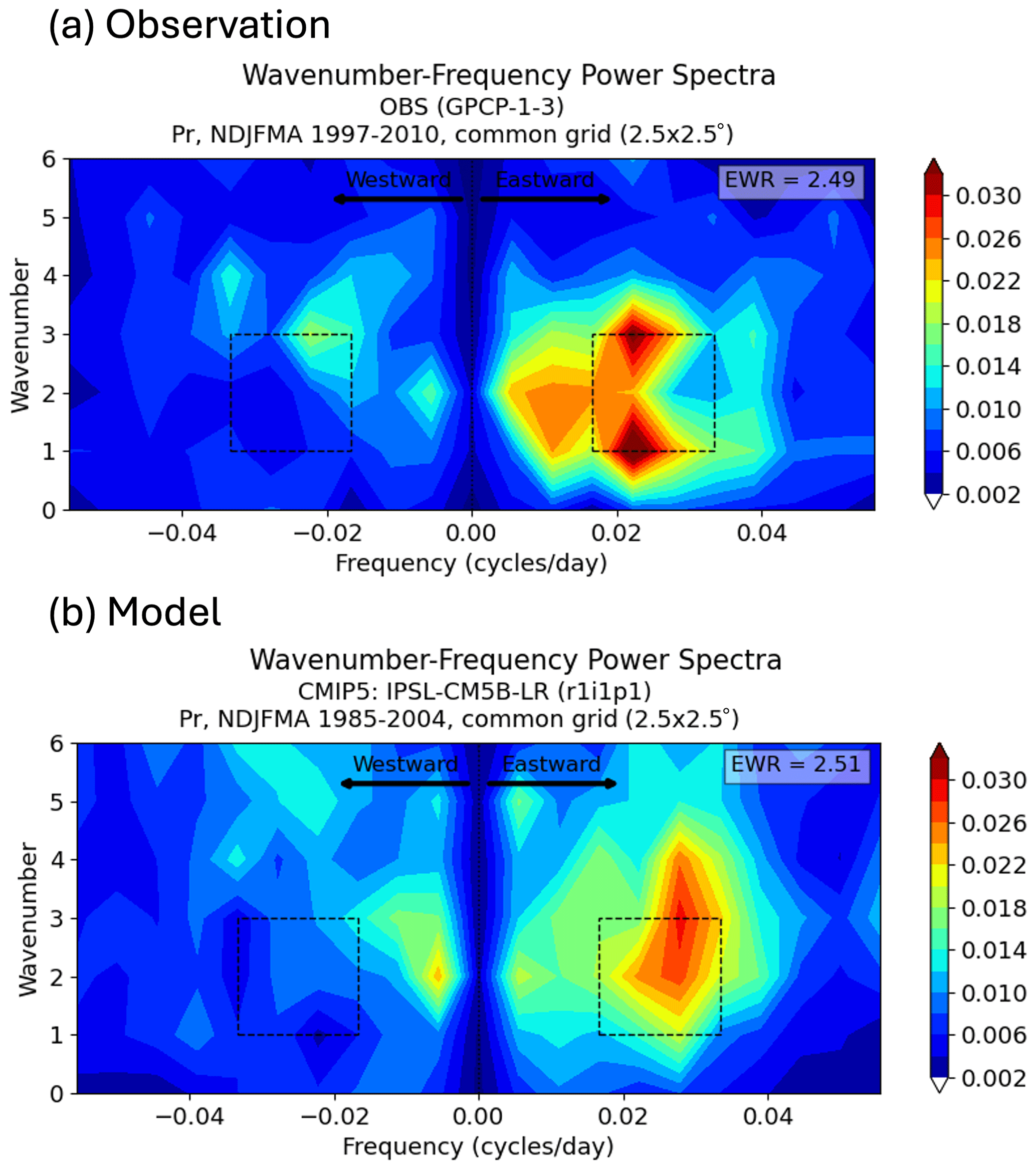
Figure 5 MJO EWR diagnostics – wavenumber–frequency power spectra – from (a) GPCP v1.3 (Huffman et al., 2001) and (b) the IPSL-CM5B-LR model of CMIP5. The EWR is defined as the ratio of eastward power (averaged in the box on the right) to westward power (averaged in the box on the left) from the 2-dimensional wavenumber–frequency power spectra of daily 10° N–10° S averaged precipitation in November to April (shaded; mm² d⁻²). Power spectra are calculated for each year and then averaged over all years of data. The units of power spectra for the precipitation is mm² d⁻² per frequency interval per wavenumber.

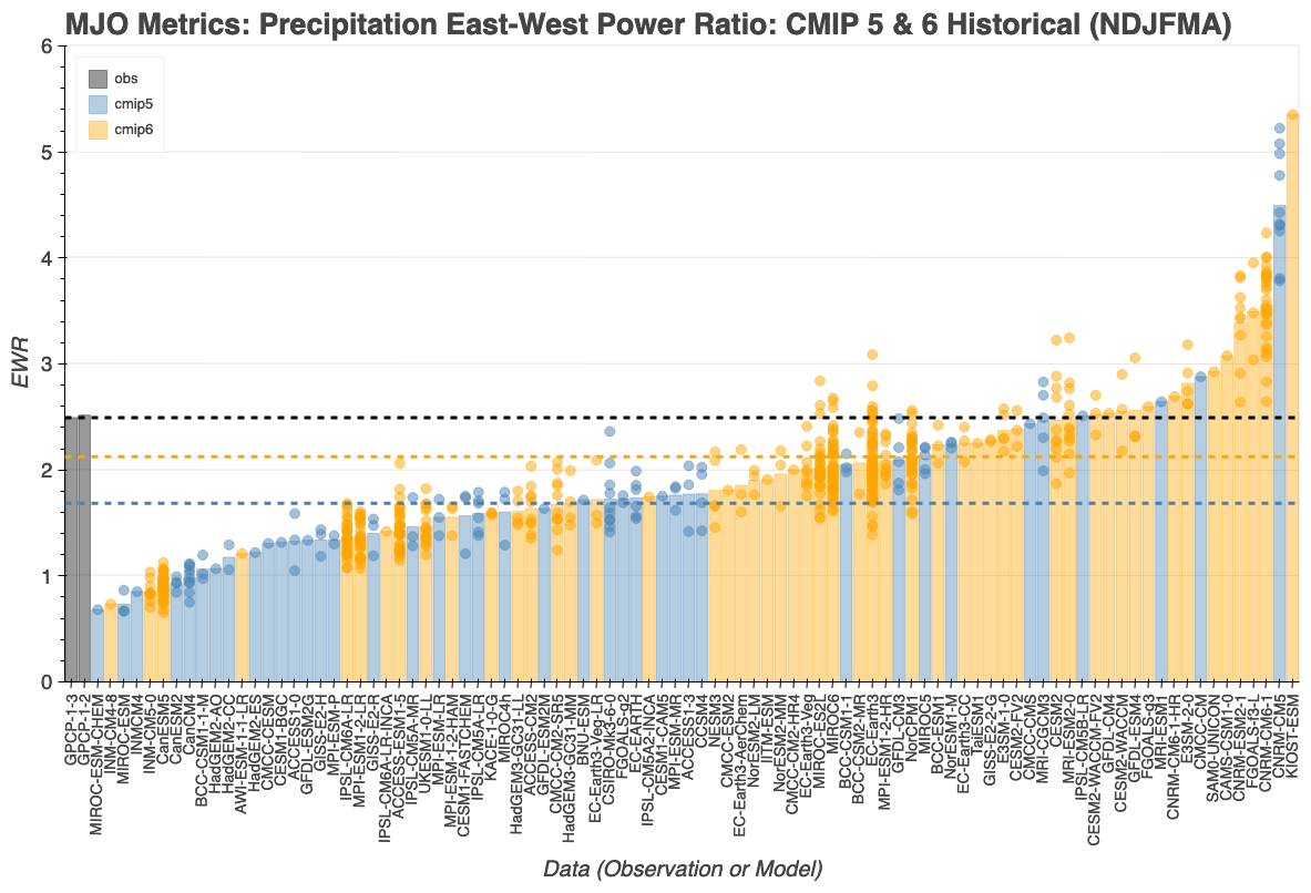
Figure 6 MJO east–west power ratio (EWR; unitless) from CMIP5 and CMIP6 models. Models in two different groups (CMIP5 – blue; CMIP6 – orange) are sorted by the value of the metric and compared to two observation datasets (purple; GPCP v1.2 and v1.3; Huffman et al., 2001). Horizontal dashed lines indicate EWR from the default primary reference observation (i.e., GPCP v1.3; black) averages of CMIP5 and CMIP6 models. The interactive plot is available at https://pcmdi.llnl.gov/research/metrics/mjo/ (last access: 8 May 2024), where the horizontal axis can be re-sorted by the CMIP group or model names as well. Hovering the mouse cursor over the boxes will show tool tips for metric values and a preview of the dive-down plots that are shown in Fig. 5.

Figure 6 shows the EWR from individual models' multiple ensemble members and their average. The average EWR of the CMIP6 model simulations is more realistic than that of the CMIP5 models. Interestingly, a substantial spread exists across models and also among ensemble members of a single model. For example, while the average EWR value for the CESM2 ensemble is 2.47 (close to 2.49 from the GPCP observations), the EWR values of the individual ensemble members range from 1.87 to 3.23. Kang et al. (2020) suggested that the ensemble spread in the propagation characteristics of the MJO can be attributed to the differences in the moisture mean state, especially its meridional moisture gradient. A cautionary note should be given to the fact that the MJO frequency and wavenumber windows are chosen to capture the spectral peak in observations. Thus, while the EWR provides an initial evaluation of the propagation characteristics of the observed and simulated MJO, it is instructive to look at the frequency–wavenumber spectra, as in some cases the dominant periodicity and wavenumber in a model may be different than in observations. It is worthwhile to note that the PMP can be used to obtain EWR and EOR of other daily variables for MJO analysis, such as outgoing longwave radiation (OLR) or zonal wind at 850 hPa (U-850) or 250 hPa (U-250), as shown in Ahn et al. (2017).

3.5 Monsoons

Based on the work of Sperber and Annamalai (2014), skill metrics in the PMP quantify how well models represent the onset, decay, and duration of regional monsoons. From observations and Historical simulations, the climatological pentad data of precipitation are area-averaged for six monsoon domains: all-India rainfall, Sahel, Gulf of Guinea, North American monsoon, South American monsoon, and northern Australia (Fig. 7). For the domains in the Northern Hemisphere, the 73 climatological pentads run from January to December, while for the domains in the Southern Hemisphere, the pentads run from July to June. For each domain, the precipitation is accumulated at each subsequent pentad and then divided by the total precipitation to give the fractional accumulation of precipitation as a function of pentad. Thus, the annual cycle behavior is evaluated irrespective of whether a model has a dry or wet bias. Except for the Gulf of Guinea, the onset and decay of monsoon occur for a fractional accumulation of 0.2 and 0.8, respectively. Between these fractional accumulations, the accumulation of precipitation is nearly linear as the monsoon season progresses. Comparison of the simulated and observed onset, duration, and decay are presented in terms of the difference in the pentad index obtained from the model and observations (i.e., model minus observations). Therefore, negative values indicate that the onset or decay in the model occurs earlier than in observations, while positive values indicate the opposite. For duration, negative values indicate that for the model it takes fewer pentads to progress from onset to decay compared to observations (i.e., the simulated monsoon period is too short), while positive values indicate the opposite.

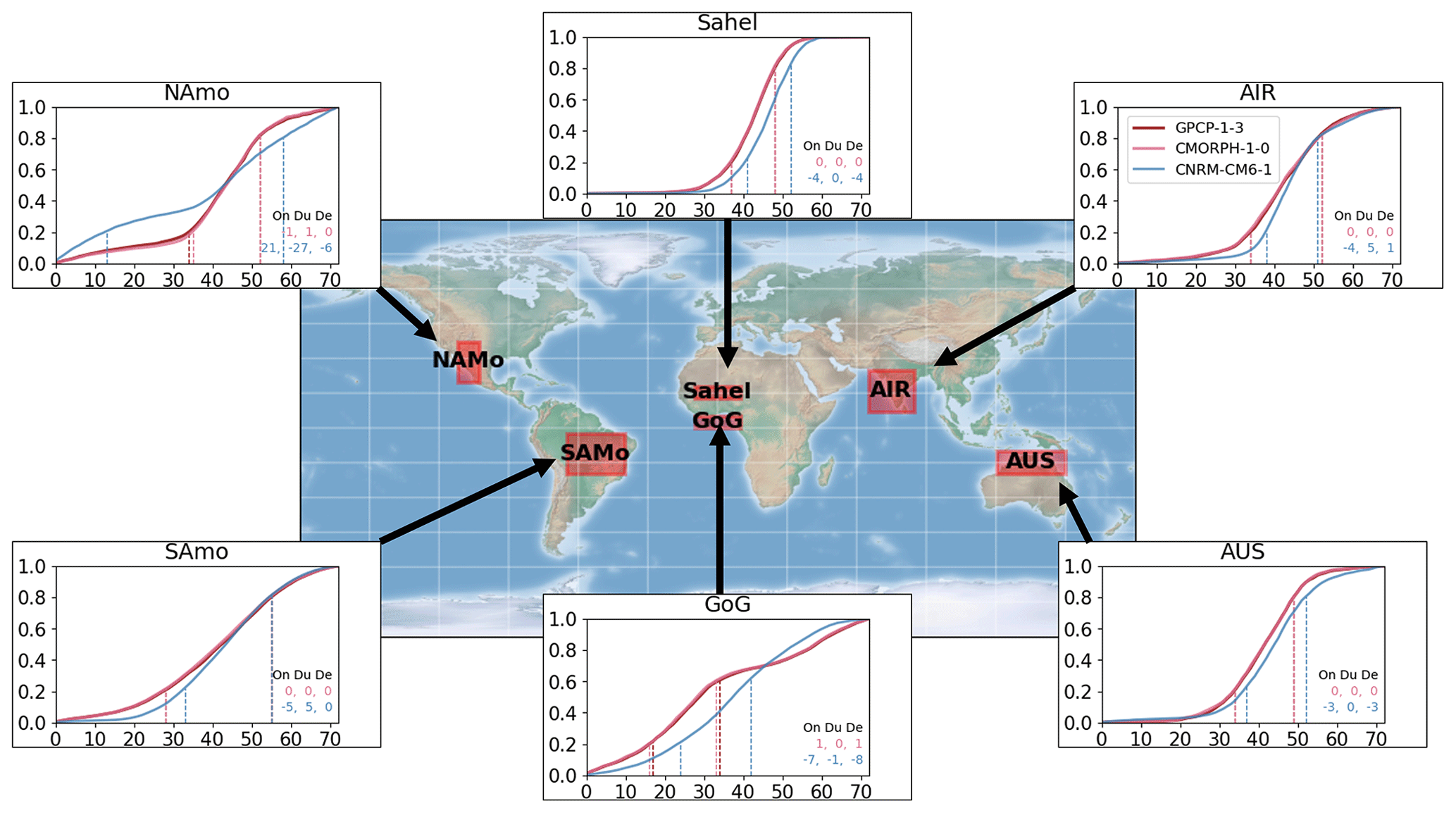
Figure 7 Demonstration of the monsoon metrics obtained from observation datasets (GPCP v1.3 and CMORPH v1.0; Joyce et al., 2004; Xie et al., 2017) and a CMIP6 model's Historical simulation conducted using CNRM-CM6-1. The results are obtained for monsoon regions: all-India rainfall (AIR), Sahel, Gulf of Guinea (GoG), North American monsoon (NAM), South American monsoon (SAM), and northern Australia (AUS). The regions are defined in Sperber and Annamalai (2014). Metrics for onset (On), duration (Du), and decay (De) derived as differences to the default observation (GPCP v1.3) in pentad indices (observation minus model) are shown at lower right of each panel. Pentad indices for the onset and decay of each region are also shown as vertical lines.

For CMIP5, we find systematic errors in the phase of the annual cycle of rainfall. The models are delayed in the onset of summer rainfall over India, the Gulf of Guinea, and the South American monsoon, with early onset prevalent for the Sahel and the North American monsoon. The lack of consistency in the phase error across all domains suggests that a “global” approach to the study of monsoons may not be sufficient to rectify the regional differences. Rather, regional process studies are necessary for diagnosing the underlying causes of the regionally specific systematic model biases over the different monsoon domains. Assessment of the monsoon fidelity in CMIP6 models using the PMP is in progress.

3.6 Cloud feedback and mean state

Uncertainties in cloud feedback are the primary driver of model-to-model differences in climate sensitivity – the global temperature response to a doubling of atmospheric CO₂. Recently, an expert synthesis of several lines of evidence spanning theory, high-resolution models, and observations was conducted to establish quantitative benchmark values (and uncertainty ranges) for several key cloud feedback mechanisms. The assessed feedbacks are those due to changes in high-cloud altitude, tropical marine low-cloud amount, tropical anvil cloud area, land cloud amount, middle-latitude marine low-cloud amount, and high-latitude low-cloud optical depth. The sum of these six components yields the total assessed cloud feedback, which is part of the overall radiative feedback that fed into the Bayesian calculation of climate sensitivity in Sherwood et al. (2020). Zelinka et al. (2022) estimated these same feedback components in climate models and evaluated them against the expert-judgment values determined in Sherwood et al. (2020), ultimately deriving a root mean square error metric that quantifies the overall match between each model's cloud feedback and those determined through expert judgment.

Figure 8 shows the model-simulated values for each individual feedback computed in amip-p4K simulations as part of CMIP5 and CMIP6 alongside the expert-judgment values. Each model is color-coded by its equilibrium climate sensitivity (determined using abrupt-4xCO2 simulations, as described in Zelinka et al., 2020), and the values from an illustrative model (GFDL-CM4) are highlighted. Among the key results apparent from this figure is that models typically underestimate the strength of both positive tropical marine low-cloud feedback and the negative anvil cloud feedback relative to the central expert assessed value. The sum of all six assessed feedback components is positive in all but two models, with a multi-model mean value that is close to the expert-assessed value but exhibits substantial inter-model spread.

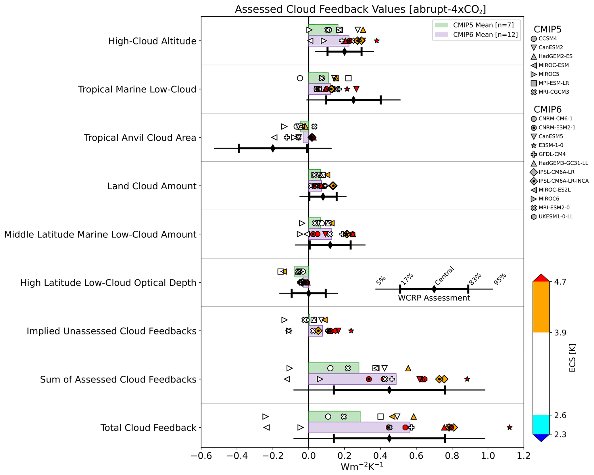
Figure 8 Cloud feedback components estimated in amip-p4K simulations from CMIP5 and CMIP6 models. Symbols indicate individual model values, while horizontal bars indicate multi-model means. Each model is color-coded by its equilibrium climate sensitivity (ECS), with color boundaries corresponding to the likely and very likely ranges of ECS, as determined in Sherwood et al. (2020). Each component's expert-assessed likely and very likely confidence intervals is indicated with black error bars. An illustrative model (GFDL-CM4) is highlighted.

In addition to evaluating the ability of models to match the assessed cloud feedback components, Zelinka et al. (2022) investigated whether models with fewer erroneous mean-state clouds tend to have smaller errors in their overall cloud feedback RMSE. This involved computing the mean state cloud property error metric developed by Klein et al. (2013). This error metric quantifies the spatiotemporal error in climatological cloud properties for clouds with optical depths greater than 3.6, weighted by their net top-of-atmosphere (TOA) radiative impact. The observational baseline against which the models are compared comes from the International Satellite Cloud Climatology Project H-series Gridded Global (ISCCP HGG) dataset (Young et al., 2018). Zelinka et al. (2022) showed that models with smaller mean state cloud errors tend to have stronger but not necessarily better (less erroneous) cloud feedback, which suggests that improving mean state cloud properties does not guarantee improvement in the cloud response to warming. However, the models with the smallest errors in cloud feedback tend also to have fewer erroneous mean state cloud properties, and no models with poor mean state cloud properties have feedback in good agreement with expert judgment.

The PMP implementation of this code computes cloud feedback by differentiating fields from amip-p4K and amip experiments and normalizing by the corresponding global mean surface temperature change rather than from differentiating abrupt-4xCO2 and PiControl experiments and computing feedback via regression (as was done in Zelinka et al., 2022). This choice is made to reduce the computational burden and also because cloud feedbacks derived from these simpler atmosphere-only simulations have been shown to closely match those derived from fully coupled quadrupled CO₂ simulations (Qin et al., 2022). The code produces figures in which the user-specified model results are highlighted and placed in the context of the CMIP5 and CMIP6 multi-model results (e.g., Fig. 8).

3.7 Precipitation

Recognizing the importance of accurately simulating precipitation in ESMs and a lack of objective and systematic benchmarking for it and being motivated by discussions with WGNE and WGCM working groups of WCRP, the DOE has initiated an effort to establish a pathway to help modelers gauge improvement (U.S. DOE, 2020). The 2019 DOE workshop “Benchmarking Simulated Precipitation in Earth System Models” generated two sets of precipitation metrics: baseline and exploratory metrics (Pendergrass et al., 2020). In the PMP, we have focused on implementing the baseline metrics for benchmarking simulated precipitation. In parallel, a set of exploratory metrics that could be added to metric suites, including PMP, in the future was illustrated by Leung et al. (2022) to extend the evaluation scope to include process-oriented and phenomena-based diagnostics and metrics.

The baseline metrics gauge the consistency between ESMs and observations, focusing on the holistic set of observed rainfall characteristics (Fig. 9). For example, the spatial distribution of mean state precipitation and seasonal cycle are outcomes of the PMP's climatology metrics (described in Sect. 3.1) which provide collective evaluation statistics such as RMSE, standard deviation, and pattern correlation over various domains (e.g., global, NH and SH extratropics, and tropics, with each domain as a whole, and over land and ocean, in separate domains). Evaluation of precipitation variability across many timescales with PMP is documented in Ahn et al. (2022); we summarize some of the findings here. The precipitation variability metric measures forced (diurnal and annual cycles) and internal variability across timescales (subdaily, synoptic, subseasonal, seasonal, and inter-annual) in a framework based on power spectra of 3 h total and anomaly precipitation. Overall, CMIP5 and CMIP6 models underestimate the internal variability, which is more pronounced in the higher-frequency variability, while they overestimate the forced variability (Fig. 10). For the diurnal cycle, PMP includes metrics from Covey et al. (2016). Additionally, the intensity and distribution of precipitation are assessed following Ahn et al. (2023). Extreme daily precipitation indices and their 20-year return values are calculated using a non-stationary generalized extreme value statistical method. From the CMIP5 and CMIP6 historical simulations, we evaluate model performance of these indices and their return values in comparison with gridded land-based daily observations. Using this approach, Wehner et al. (2020) found that at the models' standard resolutions, no meaningful differences were found between the two generations of CMIP models. Wehner et al. (2021) extended the evaluation of simulated extreme precipitation to seasonal 3 h precipitation extremes produced by available HighResMIP models and concluded that the improvement is minimal with the models' increased spatial resolutions. They also noted that the order of operations of regridding and calculating extremes affects the ability of models to reproduce observations. Drought metrics developed by Xue and Ullrich (2021) are not implemented in PMP directly but are wrapped by the Coordinated Model Evaluation Capabilities (CMEC; Ordonez et al., 2021), which is a parallel framework for supporting community-developed evaluation packages. Together, these metrics provide a streamlined workflow for running the entire baseline metrics via the PMP and CMEC that is ready for use by operational centers and in the CMIP7.

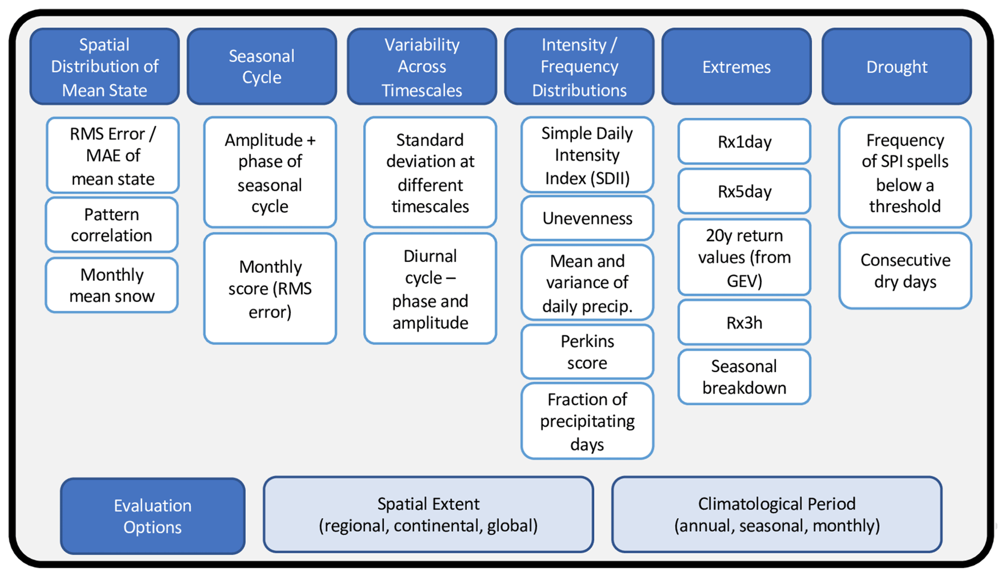
Figure 9 Proposed suite of baseline metrics for simulated precipitation benchmarking (figure reprinted from workshop report; U.S. DOE, 2020).

3.8 Relating metrics to underlying diagnostics

Considering the extensive collection of information generated from the PMP, efforts have supported improved visualizations of metrics using interactive graphical user interfaces. These capabilities can facilitate the interpretation and synthesis of vast amounts of information associated with the diverse metrics and the underlying diagnostics from which they were derived. Via the interactive navigation interface, we can explore the underlying diagnostics behind the PMP's summary plots. On the PCMDI website, we provide interactive graphical interfaces to enable navigating the supporting plots to the underlying diagnostics of each model's ensemble members and their average. For example, for the interactive mean climate plots (https://pcmdi.llnl.gov/metrics/mean_clim/, last access: 8 May 2024), hovering the mouse cursor over a square or triangle in the portrait plot, or over the markers or lines in the parallel coordinate plot, reveals the diagnostic plot from which the metrics were generated. It allows the user to toggle between several metrics (e.g., RMSE, bias, and correlation) and regions (e.g., global, Northern/Southern hemispheres, and tropics), along with relevant provenance information. Users can click on the interactive plots to get dive-down diagnostics information for the model of interest which provides detailed analysis to better understand how the metric was calculated. As with the PMP's mean climate metrics output, we currently provide interactive summary graphics for ENSO (https://pcmdi.llnl.gov/metrics/enso/, last access: 8 May 2024), extratropical modes of variability (https://pcmdi.llnl.gov/metrics/variability_modes/, last access: 8 May 2024), monsoon (https://pcmdi.llnl.gov/metrics/monsoon/, last access: 8 May 2024), MJO (https://pcmdi.llnl.gov/metrics/mjo/, last access: 8 May 2024), and precipitation benchmarking (https://pcmdi.llnl.gov/metrics/precip/, last access: 8 May 2024). We plan to expand this capability to other metrics in the PMP, such as the cloud feedback analysis. The majority of the PMP's interactive plots have been developed using Bokeh (https://bokeh.org/, last access: 8 May 2024), a Python data visualization library that enables the creation of interactive plots and applications for web browsers.

4 Model benchmarking

While the PMP originally focused on evaluating multiple models (e.g., Gleckler et al., 2008), in parallel there has been increasing interest from model developers and modeling centers to leverage the PMP to track performance evolution in the model development cycle, as discussed in Gleckler et al. (2016). For example, metrics from the PMP have been used to document performance of ESMs developed in the U.S. DOE Exascale Earth System Model (E3SM; Caldwell et al., 2019; Golaz et al., 2019; Rasch et al., 2019; Hannah et al., 2021; Tang et al., 2021), NOAA Geophysical Fluid Dynamics Laboratory (GFDL; Zhao et al., 2018), Institut Pierre-Simon Laplace (IPSL; Boucher et al., 2020; Planton et al., 2021), National Institute of Meteorological Sciences–Korea Meteorological Administration (NIMS–KMA; Sung et al., 2021), University of California, Los Angeles (Lee et al., 2019b), and the Community Integrated Earth System Model (CIESM) project (Lin et al., 2020).

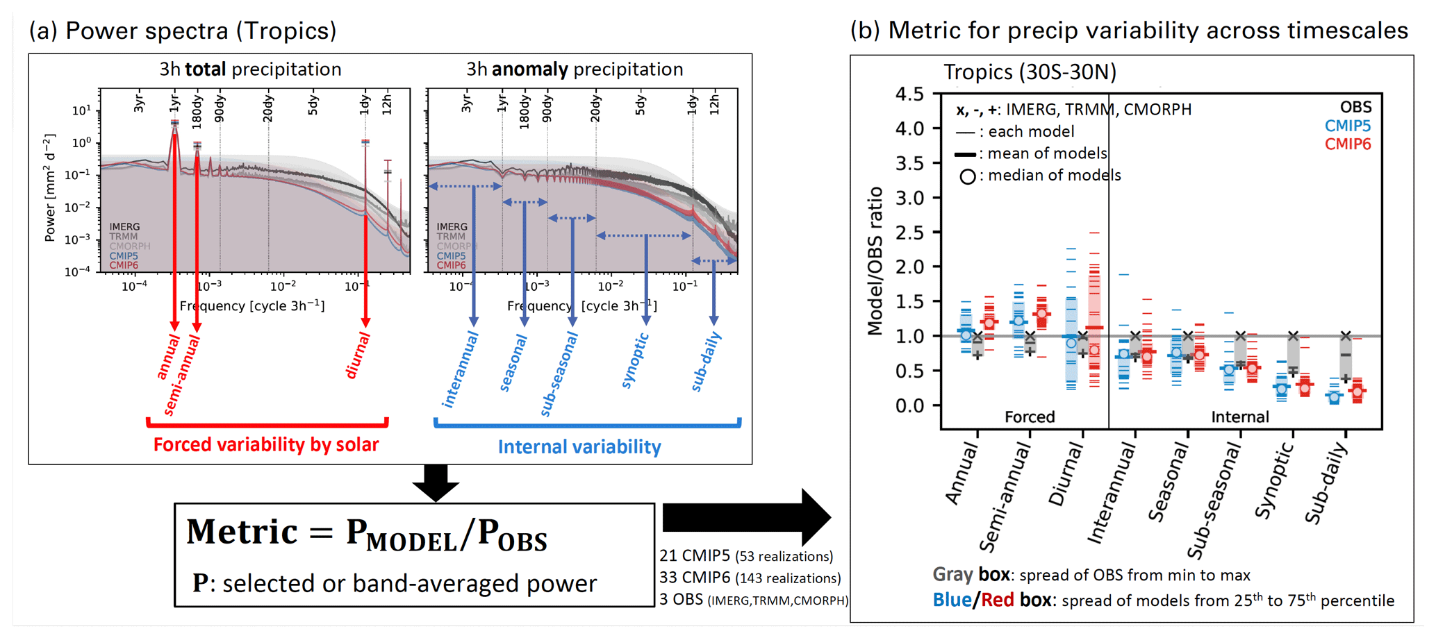
Figure 10 Example of (a) an underlying diagnostic and (b) its resulting metrics for precipitation variability across timescales. (a) Power spectra of 3 h total (left) and anomaly (right) precipitation from IMERG (black), TRMM (gray), CMORPH (silver), CMIP5 (blue), and CMIP6 (red) averaged over the tropics (30° S–30° N). The colored shading indicates the 95 % confidence interval for each observational product and for the CMIP5 and CMIP6 means. (b) Metrics for forced and internal precipitation variability are based on power spectra. The reference observational product displayed is GPM IMERG (Huffman et al., 2015). The gray boxes represent the spread of the three observational products (“X” for IMERG, “−” for TRMM, and “+” for CMORPH) from the minimum to maximum values. Blue and red boxes indicate the 25th to the 75th percentile of CMIP models as a measure of spread. Individual models are shown as thin dashes, the multi-model mean as a thick dash, and the multi-model median as an open circle. Details of the diagnostics and metrics are described in Ahn et al. (2022).

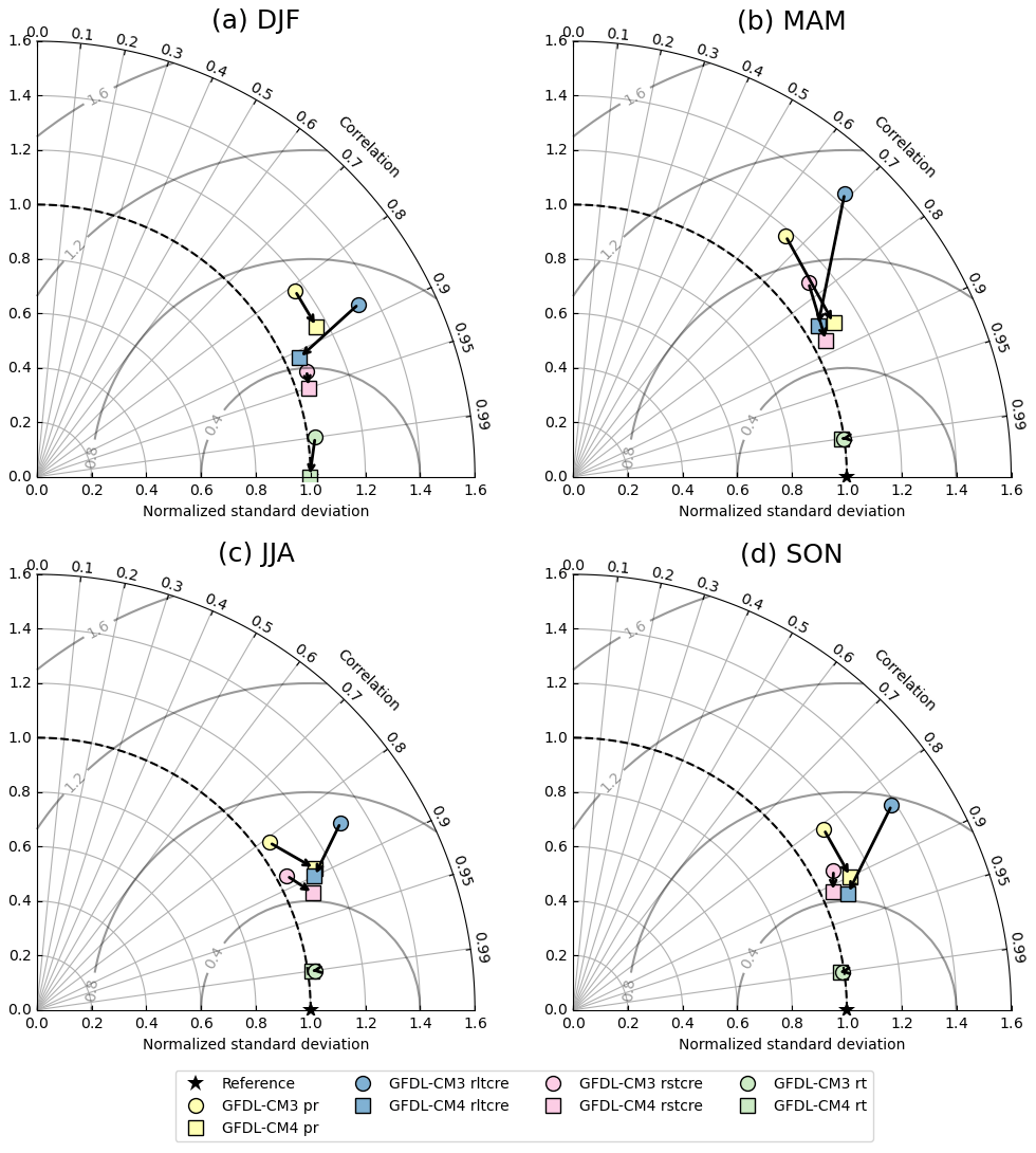
Figure 11 Taylor diagram contrasting performance of an ESM in their two different versions (i.e., GFDL-CM3 from CMIP5 and GFDL-CM4 from CMIP6) in its Historical simulation for multiple variables (precipitation [pr], longwave cloud radiative effect [rltcre], shortwave cloud radiative effect [rstcre], and total radiation flux [rt]) in their climatology over the globe for (a) December–February (DJF), (b) March–May (MAM), (c) June–August (JJA), and (d) September–November (SON) seasons. The arrow is directed toward the newer version of the model from the older version (i.e., GFDL-CM3 → GFDL-CM4).

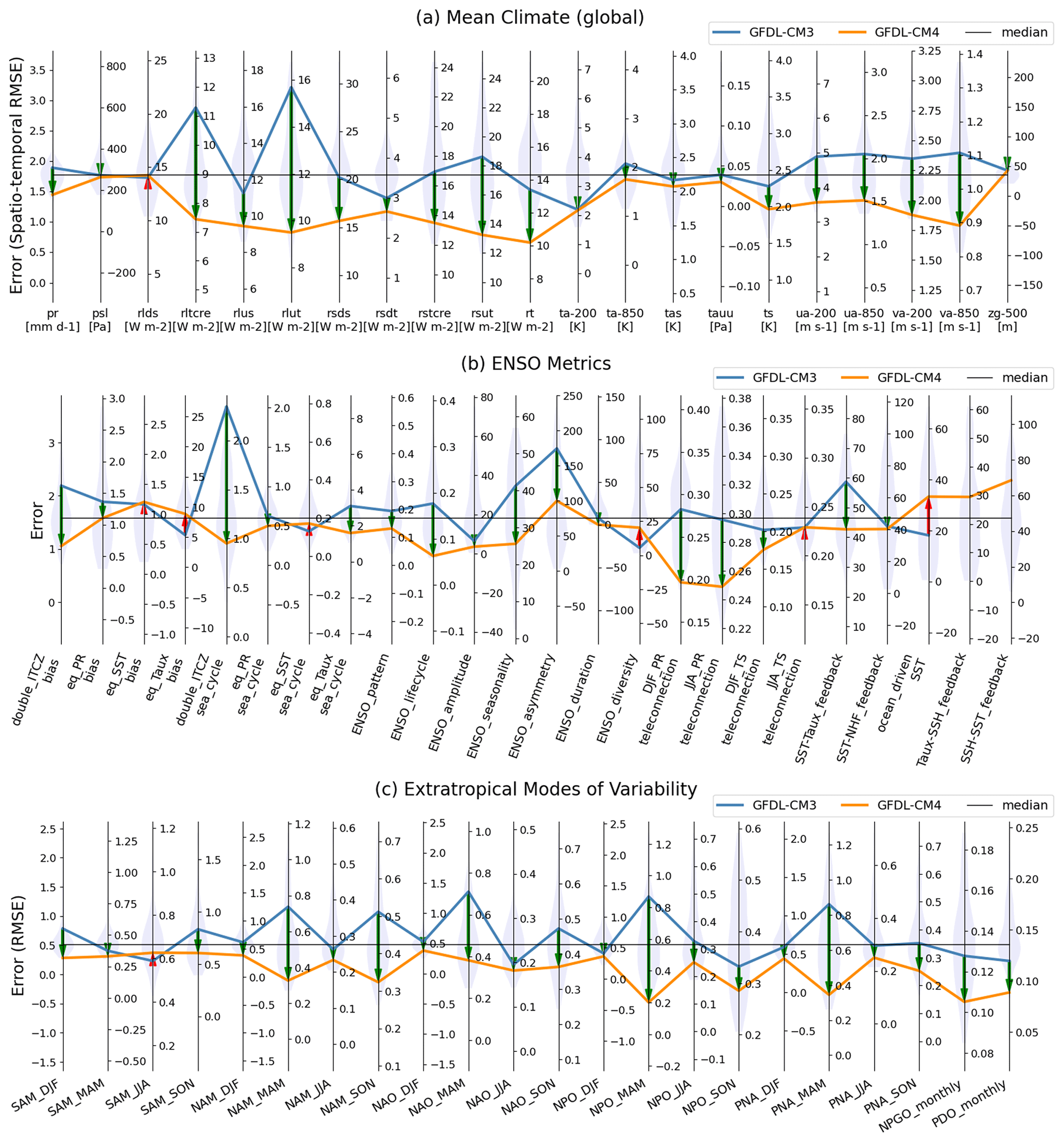
Figure 12 Parallel coordinate plot contrasting the performance of two different versions of the GFDL model (i.e., GFDL-CM3 from CMIP5 and GFDL-CM4 from CMIP6) in their Historical experiment for errors from (a) mean climate, (b) ENSO, and (c) extratropical modes of variability. Improvement (degradation) in the later version of the model is highlighted as a downward green (upward red) arrow between lines. The middle of each vertical axis is set to the median of the group of benchmarking models (i.e., CMIP5 and CMIP6), with the axis range stretched to maximum distance to either minimum or maximum from the median for visual consistency. The inter-model distributions of model performance are shown as shaded violin plots along each vertical axis.

To make the PMP more accessible and useful for modeling groups, efforts are underway to broaden workflow options. Currently, a typical application involves computing a particular class of performance metrics (e.g., mean climate) for all CMIP simulations available via ESGF. To facilitate the ability of modeling groups to routinely use the PMP during their development process, we are working to provide a customized workflow option to run all the PMP metrics more seamlessly on a single model and to compare these results with a database of PMP results obtained from CMIP simulations (see the “Code and data availability” section). Via the PMP-documented and pre-calculated metrics from simulations in the CMIP archive, it is possible to readily incorporate CMIP results into the assessment of new simulations without retrieving all CMIP simulations and recomputing the results. The resulting quick-look feedback can highlight model improvement (or deterioration) and can assist in determining development priorities or in the selection of a new model version.

As an example, here, we show PMP results obtained from GFDL-CM3 from CMIP5 and GFDL-CM4 from CMIP6 for a demonstration using the Taylor diagram to compare versions of a given model (Fig. 11). One advantage of the Taylor diagram is that it collectively represents three statistics (i.e., centered RMSE, standard deviation, and correlation) in a single plot (Taylor, 2001), which synthesizes the performance intercomparison of multiple models (or different versions of a model). In this example, four variables were selected to summarize performance evolution (shown by arrows) in multiple seasons. Except for boreal winter, both model versions are nearly identical in terms of net TOA radiation; however, in all seasons the longwave cloud radiative effect is clearly improved in the newer model version. The TOA flux improvements likely contributed to the precipitation improvements by improving the balances of radiative cooling and latent heating. The improvement in the newer model version is consistent with that documented by Held et al. (2019) and evident via the arrow directions pointing to the observational reference point.

Parallel coordinate plots can also be used to summarize the comparison of two simulations for their performance. In Fig. 12, we demonstrate the comparison of selected metrics: the mean climate (see Sect. 3.1), ENSO (Sect. 3.2), and ETMoV (Sect. 3.3). To facilitate comparison of a subset of models, a few models can be selected and highlighted as connected lines across individual vertical axes on the plot. A proposed application of it from PMP is to select two models or two versions of a model to contrast their performance (solid lines) against the backdrop of results from other models, which are shown as violin plots for the distribution of statistics from other models on each vertical axis. In this example, we contrast the performance of two GFDL models: GFDL-CM3 and GFDL-CM4. Figure 12a is a modified version of Fig. 2 that is designed to highlight the difference in performance more efficiently. Each vertical axis indicates performance for each metric defined for the climatology of variables (i.e., temporally averaged spatial RMSE of annual cycle climatology patterns; Fig. 12a), ENSO characteristics (Fig. 12b), or inter-annual variability mode obtained from seasonal or monthly averaged time series (Fig. 12c). It is shown that GFDL-CM4 is superior to GFDL-CM3 for most cases across selected metrics (downward arrows in green), while inferior for a few cases (upward arrows in red), which is consistent with previous findings (Held et al., 2019; Planton et al., 2021; Chen et al., 2021). Such applications of the parallel coordinate plot can enable quick overall assessment and tracking of the ESM performance evolution during its development cycle. More examples showing other models are available in the Supplement (Figs. S1 to S3).

It is worth noting that there have been efforts to coalesce objective model evaluation concepts used in the research community (e.g., Knutti et al., 2010). However, the field continues to evolve rapidly with definitions still being debated and finessed. Via the PMP, we produce hundreds of summary statistics, enabling a broad net to be cast in the objective characterization of a simulation, at times helping modelers identify previously unknown deficiencies. For benchmarking, efforts are underway to establish a more targeted path which likely involves a consolidated set of carefully selected metrics.

5 Discussion

Efforts are underway to include new metrics into the PMP to advance the systematic objective evaluation of ESMs. For example, in coordination with the World Meteorological Organization (WMO)'s WGNE MJO Task Force, additional candidate MJO metrics for PMP inclusion have been identified to facilitate more comprehensive assessments of the MJO. Implementation of metrics for MJO amplitude, periodicity, and structure into the PMP is planned. An ongoing collaboration with NCAR aims to incorporate metrics related to the upper atmosphere, specifically the Quasi-Biennial Oscillation (QBO) and QBO–MJO metrics (e.g., Kim et al., 2020). We also have plans to grow the scope of PMP beyond its traditional atmospheric realm, for example, including the ocean and polar regions through collaboration with the U.S. DOE's project entitled High Latitude Application and Testing of ESMs (HiLAT, https://www.hilat.org/, last access: 8 May 2024). In addition, the PMP framework is also well poised to contribute to high-resolution climate modeling activities, such as the High-Resolution Model Intercomparison Project (HighResMIP; Haarsma et al., 2016) and the DYnamics of the Atmospheric general circulation Modeled On Non-hydrostatic Domains (DYAMOND; Stevens et al., 2019). This motivates the development of specialized metrics for high-resolution models, targeting the simulation features enabled by high-resolution models. Another potential avenue for the PMP involves leveraging machine learning (ML) techniques and other state-of-the-art data science techniques being used for process-oriented ESM evaluation works (e.g., Nowack et al., 2020; Labe and Barnes, 2022; Dalelane et al., 2023). Applications of ML detection, such as for storms, using TempestExtremes (Ullrich and Zarzycki 2017; Ullrich et al., 2021), and fronts (e.g., Biard and Kunkel, 2019), can enable additional specialized storm metrics for high-resolution simulations. For convection-permitting models, yet more storm metrics can be applied such as mesoscale convective systems. Atmospheric blocking metrics and atmospheric river evaluation metrics using the ML pattern detection capabilities in the latest TempestExtremes (Ullrich et al., 2021) are currently under development to be implemented into the PMP. These example enhancements of the PMP are indicative of an increasing priority to target regional simulation characteristics. With a deliberate emphasis on processes intrinsic to specific regions, this may lead to enabling potential applications of the PMP within the regional climate modeling activities such as the COordinated Regional climate Downscaling EXperiment (CORDEX; Gutowski et al., 2016).

The comprehensive database of PMP results offers a resource for exploring the range of structural errors in CMIP class models and their interrelationships. For example, examination of cross-metric relationships between mean state and variability biases can shed additional light on the propagation of errors (e.g., Kang et al., 2020; Lee et al., 2021b). There continues to be interest in ranking models for specific applications (e.g., Ashfaq et al., 2022; Goldenson et al., 2023; Longmate et al., 2023; Papalexiou et al., 2020; Singh and AchutaRao, 2020) or to “move beyond one model one vote” in multi-model analysis to reduce uncertainties in the spread of multi-model projections (e.g., Knutti, 2010; Knutti et al., 2017; Sanderson et al., 2017; Herger et al., 2018; Hausfather et al., 2022; Merrifield et al., 2023). While we acknowledge potential interests in using the results of the PMP or equivalent to rank models or identify performance outliers (e.g., Sanderson and Wehner, 2017), we believe the many challenges associated with model weighting are application-dependent and thus leave it up to users of the PMP to make those judgments.

In addition to the scientific challenges associated with diversifying objective summaries of model performance, there is potential to leverage rapidly evolving technologies, including new open-source tools and methods available to scientists. We expect that the ongoing PMP code modernization effort to fully adapt the xCDAT and xarray will facilitate greater community involvement. As the PMP evolves with these technologies, we will continue to maintain rigor in the calculation of statistics for the PMP metrics, for example, by incorporating the latest advancements in the field. A prominent example in the objective comparison of models and observations involves the methodology of horizontal interpolation, and in future versions of the PMP, we are planning a more stringent conservation method (Taylor, 2024). To improve the clarity of key messages from multivariate PMP metrics data, we will consider implementing the advances in high-dimensional data visualization, e.g., the circular plot discussed in J. Lee et al. (2018) and variations in the parallel coordinate plots proposed in this paper and by Hassan et al. (2019) and Lu et al. (2020).

Current progress towards systematic model evaluation is exemplified by the diversity of tools being developed (e.g., the PMP, ESMValTool, MDTF, ILAMB, IOMB, and other packages). Each of these tools has its own scientific priorities and technical approaches. We believe that this diversity has made, and will continue to make, the model evaluation process even more comprehensive and successful. The fact that there is some overlap in a few cases is advantageous because it enables the cross-verification of results, which is particularly useful in more complex analyses. Despite possible advantages, having no single best or widely accepted approach for the community to follow does introduce complexity to the coordination of model evaluation. To facilitate the collective usage of individual evaluation tools, the CMEC has initiated the development of a unified code base that technically coordinates the operation of distinct but complementary tools (Ordonez et al., 2021). Currently, the PMP, ILAMB, MDTF, and ASoP have become CMEC compliant by adopting common interface standards that define how evaluation tools interact with observational data and climate model output. We expect that CMEC can also help the model evaluation community to establish standards for archiving the metrics output, similar to what the community did for the conventions to describe climate model data (e.g., CMIP application of CF Metadata Conventions (http://cfconventions.org/, last access: 8 May 2024); Hassell et al., 2017; Eaton et al., 2022).

6 Summary and conclusion

The PCMDI has actively developed the PMP with support from the U.S. DOE to improve the understanding of ESMs and to provide systematic and objective ESM evaluation capabilities. With its focus on physical climate, the current evaluation categories enabled in the PMP include seasonal and annual climatology of multiple variables, ENSO, various variability modes in the climate system, MJO, monsoon, cloud feedback and mean state, and simulated precipitation characteristics. The PMP provides quasi-operational ESM evaluation capabilities that can be rapidly deployed to objectively summarize a diverse suite of model behavior with results made publicly available. This can be of value in the assessment of community intercomparisons like CMIP, the evaluation of large ensembles, or the model development process. By documenting objective performance summaries produced by the PMP and making them available via detailed version control, additional research is made possible beyond the baseline model evaluation, model intercomparison, and benchmarking. The outcomes of PMP's calculations applied to the CMIP archive culminate in the PCMDI Simulation Summary (https://pcmdi.llnl.gov/metrics/, last access: 8 May 2024) that has served as a comprehensive data portal for objective model-to-observation comparisons and model-to-model benchmarking and intercomparisons. Special attention is dedicated to the most recent ensemble of models contributing to CMIP6. By offering a diverse and comprehensive suite of evaluation capabilities, the PMP framework equips model developers with quantifiable benchmarks to validate and enhance model performance.

We expect that the PMP will continue to play a crucial role in benchmarking ESMs. Improvements in the PMP, along with progress in interconnected model intercomparison project (MIP) community projects, will greatly contribute to advancing the evaluation of ESMs, including connection to the community efforts (e.g., the CMIP Benchmarking Task Team). Enhancements in version control and transparency within obs4MIPs are set to enhance the provenance and reproducibility of the PMP results, thereby strengthening the foundation for rigorous and repeatable performance benchmarking. The PMP's collaboration with the CMIP Forcing Task Team, through the Input4MIPs (Durack et al., 2018) and the CMIP6Plus projects, will further expand the utility of performance metrics in identifying problems associated with the forcing dataset and their application and use in reproducing the observed record of historical climate. Furthermore, as ESMs advance towards more operationalized configurations to meet the demands of decision-making processes (Jakob et al., 2023), the PMP holds significant potential to provide interoperable ESM evaluation and benchmarking capabilities to the community.

Appendix A: Table of acronyms

Acronym	Description
AMIP	Atmospheric Model Intercomparison Project
AMO	Atlantic Multi-decadal Oscillation
ARM	Atmospheric Radiation Measurement
ASoP	Analyzing Scales of Precipitation
CBF	Common basis function
CDAT	Community Data Analysis Tools
CIESM	Community Integrated Earth System Model
CLIVAR	Climate and Ocean Variability, Predictability and Change
CMEC	Coordinated Model Evaluation Capabilities
CMIP	Coupled Model Intercomparison Project
CMOR	Climate Model Output Rewriter
CVDP	Climate Variability Diagnostics Package
DOE	U.S. Department of Energy
ENSO	El Niño–Southern Oscillation
EOF	Empirical orthogonal function
EOR	East power normalized by observation
ESGF	Earth System Grid Federation
ESM	Earth system model
ESMAC Diags	Earth System Model Aerosol–Cloud Diagnostics
ETMoV	Extratropical modes of variability
EWR	East : west power ratio
GFDL	Geophysical Fluid Dynamics Laboratory
ILAMB	International Land Model Benchmarking
IOMB	International Ocean Model Benchmarking
IPCC	Intergovernmental Panel on Climate Change
IPSL	Institut Pierre-Simon Laplace
ISCCP HGG	International Satellite Cloud Climatology Project H-series Gridded Global
ITCZ	Intertropical Convergence Zone
JSON	JavaScript Object Notation
MAE	Mean absolute error
MDTF	Model Diagnostics Task Force
MIPs	Model Intercomparison Projects
MJO	Madden–Julian Oscillation
NAM	Northern Annular Mode
NAO	North Atlantic Oscillation
NASA	National Aeronautics and Space Administration
NCAR	National Center for Atmospheric Research
NetCDF	Network Common Data Form
NH	Northern Hemisphere
NIMS–KMA	National Institute of Meteorological Sciences–Korea Meteorological Administration
NOAA	National Oceanic and Atmospheric Administration
NPGO	North Pacific Gyre Oscillation
NPO	North Pacific Oscillation
PCMDI	Program for Climate Model Diagnosis and Intercomparison
PDO	Pacific Decadal Oscillation
PMP	PCMDI Metrics Package
PNA	Pacific North America pattern
RCMES	Regional Climate Model Evaluation System
RMSE	Root mean square error
SAM	Southern Annular Mode
SH	Southern Hemisphere
SST	Sea surface temperature
TOA	Top of atmosphere
WCRP	World Climate Research Programme
WGCM	Working Group on Coupled Models
WGNE	Working Group on Numerical Experimentation
xCDAT	Xarray Climate Data Analysis Tools