the Creative Commons Attribution 4.0 License.
the Creative Commons Attribution 4.0 License.
 | 15 May 2024
Three-dimensional variational assimilation with a multivariate background error covariance for the Model for Prediction Across Scales – Atmosphere with the Joint Effort for Data assimilation Integration (JEDI-MPAS 2.0.0-beta)
Benjamin Ménétrier
Chris Snyder
Zhiquan Liu
Jonathan J. Guerrette
Junmei Ban
Ivette Hernández Baños
Yonggang G. Yu
William C. Skamarock
This paper describes the three-dimensional variational (3D-Var) data assimilation (DA) system for the Model for Prediction Across Scales – Atmosphere with the Joint Effort for Data assimilation Integration (JEDI-MPAS). Its core element is a multivariate background error covariance implemented through multiple linear variable changes, including a wind variable change from stream function and velocity potential to zonal- and meridional-wind components, a vertical linear regression representing wind–mass balance, and multiplication by a diagonal matrix of error standard deviations. The univariate spatial correlations for the “unbalanced” variables utilize the Background error on Unstructured Mesh Package (BUMP), which is one of the generic components in the JEDI framework. The variable changes and univariate correlations are modeled directly on the native MPAS unstructured mesh. BUMP provides utilities to diagnose parameters of the covariance model, such as correlation lengths, from an ensemble of forecast differences, though some manual adjustment of the parameters is necessary because of mismatches between the univariate correlation function assumed by BUMP and the correlation structure in the sample of forecast differences. The resulting multivariate covariances, as revealed by single-observation tests, are qualitatively similar to those found in previous global 3D-Var systems. Month-long cycling DA experiments using a global quasi-uniform 60 km mesh demonstrate that 3D-Var, as expected, performs somewhat worse than a pure ensemble-based covariance, while a hybrid covariance, which combines that used in 3D-Var with the ensemble covariance, significantly outperforms both 3D-Var and the pure ensemble covariance. Due to its simple workflow and minimal computational requirements, the JEDI-MPAS 3D-Var system can be useful for the research community.
- Article
(4072 KB) - Full-text XML
- BibTeX
- EndNote


In the 1990s, three-dimensional variational (3D-Var) data assimilation (DA) became the algorithm of choice in operational numerical weather prediction centers (Parrish and Derber, 1992; Andersson et al., 1998; Gauthier et al., 1999; Lorenc et al., 2000), owing to its numerous advantages relative to earlier optimal-interpolation assimilation schemes. The 3D-Var system is no longer widely used operationally, both because its natural development path is to four-dimensional variational assimilation (Rabier et al., 2000; Rawlins et al., 2007) and because of the rapid development of ensemble data assimilation in the last 2 decades, including ensemble-variational techniques that employ sample covariances from a forecast ensemble within the variational framework (Lorenc, 2003; Buehner, 2005). The central components of 3D-Var systems, however, are so-called static covariance models (Bannister, 2008) that provide computationally tractable representations of complex spatial and multivariate covariances, and these remain in wide use to provide background covariances for 4D-Var and as part of hybrid techniques that consider background covariance matrices that are the sum of a static covariance and an ensemble-based covariance (Hamill and Snyder, 2000).
This paper documents 3D-Var and its associated static background covariance model for JEDI-MPAS, a data assimilation system using software infrastructure from the Joint Effort for Data assimilation Integration (JEDI; Trémolet and Auligné, 2020) and the Model for Prediction Across Scales – Atmosphere (MPAS; Skamarock et al., 2012). Two companion papers are Liu et al. (2022), which gives an overview of JEDI-MPAS and initial results from a three-dimensional ensemble-variational (3DEnVar) scheme, and Guerrette et al. (2023), which documents an ensemble of data assimilations (EDA) for JEDI-MPAS.
Our motivation for implementing 3D-Var is twofold. First, JEDI-MPAS is intended for use not only in our research, but also by the broader research community. The minimal computational cost of 3D-Var and its simple workflow make it well suited where computing is a strong constraint and when introducing new users to the system. Experience with WRFDA (Barker et al., 2012), our existing community DA system, has shown that 3D-Var is often preferred by users. Equally importantly, the static covariance model from 3D-Var can be used in hybrid ensemble-variational assimilation schemes that are known to outperform 3DEnVar alone (Wang et al., 2008; Buehner et al., 2013; Clayton et al., 2013; Kuhl et al., 2013). We show the same result for JEDI-MPAS here (see also Guerrette et al., 2023).
The formulation of the static covariance model employed here has both familiar and novel elements. We generally follow Wu et al. (2002), including (i) our choice of analysis variables, (ii) the use of linear regression from a training data set to define the approximate mass-wind balances that implicitly determine the multivariate structure of the covariances (see also Derber and Bouttier, 1999), and (iii) representing univariate correlations directly on the forecast model's grid (or mesh, in the case of MPAS). Products of vectors with the univariate spatial correlation matrices, however, are computed directly on a thinned subset of the MPAS mesh and interpolated to the full-resolution mesh using the Background error on Unstructured Mesh package (BUMP; Ménétrier, 2020). This study is the first evaluation of BUMP for use in atmospheric DA.
The outline of the paper is as follows. In the next section, we give an overview of JEDI-MPAS as configured for 3D-Var. Section 3 describes the formulation of the static background covariances and their tuning using BUMP capabilities and a training data set of forecast differences. Section 4 presents single-observation tests that illustrate the structure of the implied multivariate covariances. In Sect. 5, we summarize results from cycling DA experiments with 3D-Var and a hybrid scheme, which provide an overall evaluation of the effectiveness of the JEDI-MPAS static covariances. Section 6 concludes and offers ideas for further refinements of the static covariances.
2.1 The forecast model
MPAS is described in detail in Skamarock et al. (2012), or see Liu et al. (2022) for a more concise summary. Briefly, MPAS integrates the nonhydrostatic equations of motion cast in a height-based, terrain-following vertical coordinate and using dry density and a modified moist potential temperature as thermodynamic variables. The equations are discretized on an unstructured mesh with the normal component of horizontal velocity defined on the edges of mesh cells and other prognostic variables defined at the cell centers. MPAS supports global and regional meshes, as well as meshes with quasi-uniform or variable resolution.
In all experiments presented here, MPAS is configured with a global quasi-uniform mesh of 60 km resolution and 55 vertical levels up to a model top of 30 km. The physical parameterizations are those of the “mesoscale reference” suite, as listed in Table 2 of Liu et al. (2022).
2.2 The DA system
JEDI-MPAS implements various abstract classes for MPAS within the JEDI framework (Trémolet, 2020). Those abstract classes reside in object-oriented prediction systems (OOPS) and comprise all the building blocks and operations on them necessary for data assimilation algorithms. JEDI also contains generic (model independent) implementations of some building blocks, including observation operators and quality control (the Unified Forward Operator, UFO), observation storage and access (the Interface for Observation Data Access, IODA), and the background error covariance matrix (the System-Agnostic Background Error Representation, SABER).
The variational application of OOPS minimizes a cost function given in Eq. (3) of Liu et al. (2022). Denoting by x the concatenation of the analysis variables across all model levels and mesh locations, the cost function measures the simultaneous fit of x to a background state xb, which is our best estimate of x before considering the observations, and to the observations y (also concatenated into a single vector) via an observation operator h(x) that maps a given state to the observation variables.
The minimization proceeds iteratively by linearizing the observation operator in the neighborhood of the latest iterate xg and computing the next iterate as the minimizer of the resulting quadratic cost function,
where is the increment relative to xg, . is the observation departure from xg; H is the linearization of h near xg; and B and R are the background and observational error covariance matrices, respectively. This incremental formulation is central to the architecture of OOPS and distinguishes increments, which can be operated on by B and H, from the full state, which is an argument to h. In what follows, increments will be indicated by variables preceded with δ.
All the minimization schemes for Eq. (1) and preconditioners available in OOPS involve only the application of B to increments, rather than its square root or inverse. For the single-observation test and cycling experiments shown later, we employ the B-preconditioned incremental variational application of OOPS and the Derber–Rosati Inexact Preconditioned Conjugate Gradient algorithm (Golub and Ye, 1999; Derber and Rosati, 1989).
2.3 Analysis variables and variable change
The analysis variables are the horizontal velocity (v), temperature (T), specific humidity (q), and surface pressure ps at the MPAS cell centers, as described in Liu et al. (2022). Transformations to other variables are necessary for some observation operators and for initial conditions for MPAS forecasts. Those transformations also follow Liu et al. (2022) but with one significant improvement when computing the dry density ρd and potential temperature θd for MPAS initial conditions.
In Liu et al. (2022), ρd and θd are computed from the analyzed T, ps, and q by assuming hydrostatic balance. Here, we instead compute increments for ρd and θd (i.e., δρd and δθd) from the increments δT, δps, and δq. This approach, which is implemented by linearizing the corresponding calculations of Liu et al. (2022, steps 3 and 4 of their Sect. 3.3), assumes hydrostatic balance only for the increments and not the full analyzed fields.
Assuming hydrostatic balance just for the increments is preferable because that balance is only approximate and, moreover, the discretized form of hydrostatic balance used in the variable transformation is not precisely equivalent to that implied by the discrete MPAS equations. Since the hydrostatic integral is computed from the surface upward, differences between the incremental and full-field formulations can be expected to accumulate with height. Consistently with this, JEDI-MPAS cycling experiments (not shown) using the new incremental update for ρd and θd exhibit reduced temperature bias in the stratosphere, especially near the model top.
The state (x) and increment (δx) objects in JEDI-MPAS are basically inherited from MPAS's “pool type” data structure. Thus, it is natural to choose the existing mesh decomposition and communication utilities of MPAS to handle the parallelism of the state and increment of JEDI-MPAS. The state and increment objects in JEDI-MPAS only contain their values on their own grid point without a halo region. The halo exchange (and its adjoint) is performed when needed, such as horizontal interpolation of the state or increment to the observation location and a linear variation transform containing the spatial derivatives.
In this section, we will present how the multivariate static background error covariance is designed for JEDI-MPAS. With a series of linear variable changes, the JEDI-MPAS analysis variables are transferred into a set of variables that are independent of each other. Then, we will describe how the B statistics (or parameters) can be trained from samples. The characteristics of diagnosed B statistics at the MPAS 60 km uniform mesh will be discussed. Lastly, we will discuss what modification is made to the diagnosed B statistics to resolve the discrepancy between the assumption and actual sample data set.
3.1 Multivariate background error covariance design
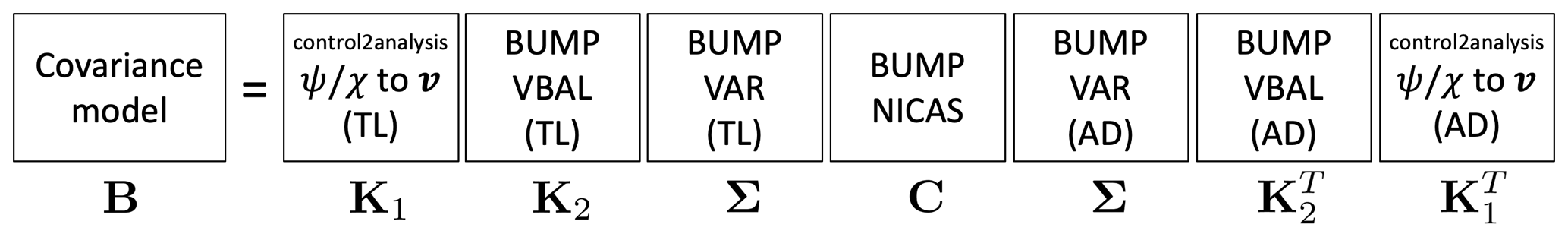
The basic design of the JEDI-MPAS multivariate background error covariance follows that of the Gridpoint Statistical Interpolation (GSI; Wu et al., 2002) system, except in our use of BUMP Normalized Interpolated Convolution from an Adaptive Subgrid (NICAS; Ménétrier, 2020), rather than recursive filters, to model the univariate spatial correlations (see further description at the end of this section). The multivariate covariances are implemented as two linear variable changes, K1 and K2, applied to a block-diagonal covariance matrix
where the block-diagonal covariance matrix has been written as the product of a block-diagonal correlation matrix C and a diagonal matrix Σ of standard deviations.
The linear variable changes K1 and K2 can be expressed in the following matrix forms.
and
Here, K1 computes increments for v from spatial derivatives (indicated schematically by the gradient terms in the upper-left block) of increments of stream function ψ and velocity potential χ. K1 and the corresponding adjoint operator, , are model-dependent JEDI components that operate on the MPAS native mesh and are implemented in Control2Analysis, a linear variable change class. Details of the calculation of v from ψ and χ are given in the Appendix.
K2 is a linear variable change that computes δχ, δT, and δps from δψ and the residual or “unbalanced” increments δχu, δTu, and δps,u (for velocity potential, temperature, and surface pressure, respectively), so called because they are by assumption independent of δψ. The relation of δχ, δT, and δps to δψ is based on linear regression from a training data set, following Derber and Bouttier (1999). As in Derber and Bouttier (1999), we choose to use δψ at a given mesh cell and on the full set of vertical levels as predictors for δT and δps at the same mesh cell and on any specific level, which makes M and N block diagonal with blocks corresponding to mesh cells and full matrices in each block. We retain δψ only on the same level as a predictor for δχ, which makes L a diagonal matrix.
Lastly, ΣCΣT is the covariance matrix for δψ; δq; and the unbalanced increments δχu, δTu, and δps,u. We assume these variables are mutually independent, so C is block diagonal with blocks that give the univariate spatial (horizontal and vertical) correlation for each variable. The matrix Σ is a diagonal matrix with elements that specify the standard deviation for δψ, δχu, δTu, dq, and δps,u.
The operations K2, , Σ, ΣT, and C use the Background error on Unstructured Mesh Package (BUMP) in the System-Agnostic Background-Error Representation (SABER) repository, which is a generic component within JEDI, through the MPAS model interfaces. The BUMP Vertical BALance (VBAL) driver is used for K2 and . It is based on the explicit vertical covariance matrices defined for a set of latitudes and is interpolated at the model grid points' latitude. The BUMP VARiance (VAR) driver is used for Σ and ΣT. It simply applies the pre-computed error standard deviations. The spatial correlation matrix is pre-computed from the given correlation lengths with BUMP–NICAS. Similarly to the GSI recursive filters, NICAS works in the grid-point space. However, it applies the convolution function explicitly, instead of recursively for GSI. Thus, the choice of the convolution function in NICAS is free, as long as it is positive definite. We choose a widely used fifth-order piecewise function of Gaspari and Cohn (1999), which resembles the Gaussian function but is compactly supported. To make the explicit convolution affordable for high-dimensional systems, it is actually performed on a low-resolution unstructured mesh. A linear interpolation is required to go from the unstructured mesh to the full model grid. Finally, an exact normalization factor is pre-computed and applied to ensure that the whole NICAS correlation operator is normalized (i.e., diagonal elements of the equivalent correlation matrix are “1”). Thus, the NICAS correlation matrix can be written as , where is the convolution operator on the low-resolution mesh, S is the interpolation from the mesh to the full model grid, and N is the diagonal normalization operator. The low-resolution mesh density can be locally adjusted depending on the diagnosed correlation lengths (or provided by the user). Figure 1 shows a diagram for Eq. (2), with corresponding BUMP drivers and MPAS-specific linear variable change.
3.2 Training the covariance model
The designed multivariate background error covariance has several parameters to be determined. These parameters are diagnosed from 366 samples of National Centers for Environmental Prediction (NCEP) Global Forecast System (GFS) 48 and 24 h forecast differences, valid at the same time of day and spanning the months of March, April, and May 2018. Here, the 24 h forecast lead time difference is chosen to remove the effect of the diurnal cycle in the perturbation samples. The GFS forecast files of 0.25° resolution on the pressure levels are interpolated to the 60 km MPAS mesh with 55 vertical levels for the following training procedures. With a recent (early June 2023) version of JEDI-MPAS source code after initial submission of this paper, we have trained the static B parameters from MPAS model's own forecast with the same methodology described here. The overall B statistics diagnosed from MPAS-based samples were similar to that from GFS-based samples reported here, except for the error standard deviations in the stratosphere, which were larger for MPAS-based samples. In the 1-month cycling experiment, this led to a reduction in temperature and wind root mean square errors (RMSEs) in 6 h forecasts in the stratosphere.
Since ΣCΣT depends on the statistics of δψ and δχ, we first need to calculate perturbations of ψ and χ from δv of each forecast difference. This is essentially the inverse operation of K1 and can be expressed as solving a Poisson equation with vorticity or divergence as a source term. Because solving a Poisson equation efficiently on the unstructured grid is not an easy task, we have adopted a spherical-harmonics-based function from the NCAR Command Language (NCL, 2019) that operates on an intermediate latitude–longitude grid. We begin by interpolating δv fields to the intermediate grid and then calculate δψ and δχ through the uv2sfvpf function of NCL and interpolate back to the MPAS mesh. Note that because the definition of δχ (shown in Eq. 3) is opposite in sign to that assumed in the NCL function, multiplying δχ (from NCL) by −1 is required.
For K2, the BUMP VBAL driver calculates the cross-variable linear regression coefficients, which are denoted as L, M, and N in Eq. (4). The vertical autocovariance matrix of δψ and the vertical cross-covariance matrices between δψ and each of δχ, δT, and δps are computed and averaged over latitude bands of ±10°. The desired matrices of regression coefficients are obtained in the standard way by right-multiplying the cross-variable covariance by the inverse autocovariance of the predictor variable (δψ in our design). The vertical autocovariance matrices are usually poorly conditioned, and thus direct computation of their inverses will yield noisy results in the presence of sampling error. To overcome this, we apply a pseudo-inverse, which only includes some dominant eigenmodes to calculate the inverse matrix. We have chosen the 20 leading modes (among a total of 55 modes) for the pseudo-inverse of the δψ autocovariance matrix.
For Σ, the BUMP VAR driver calculates variances for δψ, δχu, δTu, δq, and δps,u from the samples and filters them horizontally to damp the sampling noise. The horizontal smoother is also based on NICAS, with an appropriate mean-preserving normalization factor.
The correlation matrix, C, consists of blocks that specify the univariate spatial correlation for δψ, δχu, δTu, δq, and δps,u. The BUMP Hybrid DIAGnostic (HDIAG) driver diagnoses the horizontal and vertical correlation lengths used in modeling C parameters. HDIAG can diagnose the horizontal and vertical spatial correlations from the samples. First, it defines a low-resolution unstructured mesh. Around each mesh node, diagnostic points are randomly and isotropically drawn for different horizontal separation classes. Second, HDIAG calculates the horizontal correlation between each mesh node and its own diagnostic points from the samples, at all levels. The vertical correlation is also calculated at each mesh node, between each level and the neighboring levels. The third step is a horizontal averaging of these raw correlations, either over all the mesh nodes or over local neighborhoods. The average is binned depending on the level and the horizontal separation for the horizontal correlation and depending on the levels concerned for the vertical correlation. As a final step, HDIAG fits a Gaspari and Cohn (1999) function for each averaged correlation curve. Thus, we obtain horizontal and vertical correlation length values for each level. If the averaging and curve-fitting steps are performed over local neighborhoods, an extra interpolation step is necessary to obtain 3D fields of length scales on the model grid. These length-scale profiles or 3D fields can be stored and provided to NICAS in order to model the spatial correlation operator. In this study, the local correlation lengths were obtained from raw statistics within a 3000 km radius for a given diagnostic point.
3.3 Diagnosed statistics
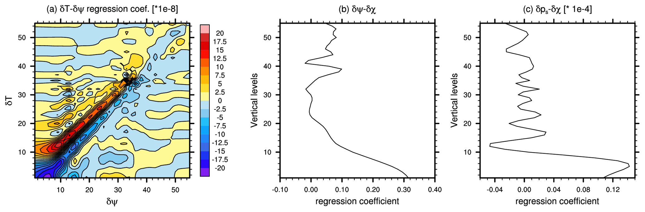
The regression coefficients that appear in the definition (4) of K2, which are computed by BUMP VBAL, are shown in Fig. 2 for a location near 34.8° N latitude. Considering first Fig. 2a, the δT–δψ coefficients are largest at small separations. Their structure is dipolar, with δT at a given level positively related to δψ at nearby but higher levels, and negatively related to δψ at nearby but lower levels. The δT–δψ coefficients are generally consistent with approximate geostrophic and hydrostatic balance, which together relate ψ to the mass field and the vertical derivative of the mass field to buoyancy. The coefficient structure is different for model levels lower than 10, perhaps due to the effects of the boundary layer and terrain. Figure 2b shows δχ–δψ coefficients, which relate δχ at a given level to δψ at the same level. The balanced part of δχ depends positively on δψ near the surface, consistent with Ekman balance, under which vertical vorticity near the surface drives horizontal convergence in the boundary layer. Finally and not unexpectedly, δps has a positive dependence on δψ in the lower troposphere (Fig. 2c).
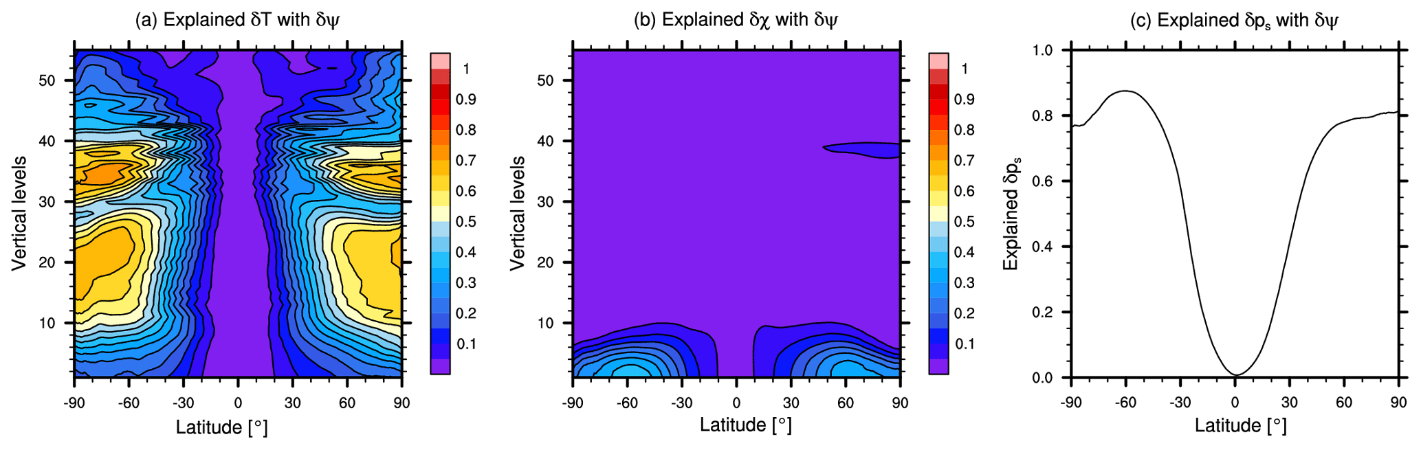
Figure 3Ratio of balanced variance (i.e., that predicted by δψ) to total variance for (a) δT, (b) δχ, and (c) δps.
Figure 3 shows the variance that can be predicted knowing δψ normalized by the total variance, for δT, δχ, and δps. There are substantial variations with latitude and height. For δT, the δT–δψ regression can explain up to 70 % of the total variance in mid-latitude and high-latitude regions in the troposphere. For δχ, the regression explains up to 35 % of the total variance in the mid-latitudes near the surface (below model level 10), while for δps, the regression explains substantial variance everywhere except the tropics. These balanced ratios are similar to those found in Wu et al. (2002) (their Fig. 1) and Barker et al. (2012) (their Fig. 5), and their geographic variations confirm that the regressions primarily reflect dynamical balances characteristic of mid-latitudes and high latitudes.
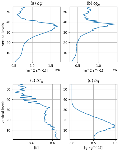
Figure 4Horizontally averaged standard deviations for (a) δψ, (b) δχu, (c) δTu, and (d) δq. The horizontally averaged standard deviation for δps,u is 53.05 Pa.
The other quantities that must be estimated from the training data set are the standard deviations that form the diagonal of Σ and the fields of horizontal and vertical correlation scales for each of the variables δψ, δχu, δTu, δq, and δps,u, which together specify the correlation matrix C. Figure 4 shows the vertical profiles of horizontally averaged standard deviations for each variable. For δψ and δχu, the standard deviation increases upward from the surface to a peak near the tropopause. The standard deviation of δTu, in contrast, generally decreases upward from a peak at the surface. For δq, the profile of standard deviations has a shape similar to that for q itself, peaked in the lower troposphere and decreasing steadily with height above.
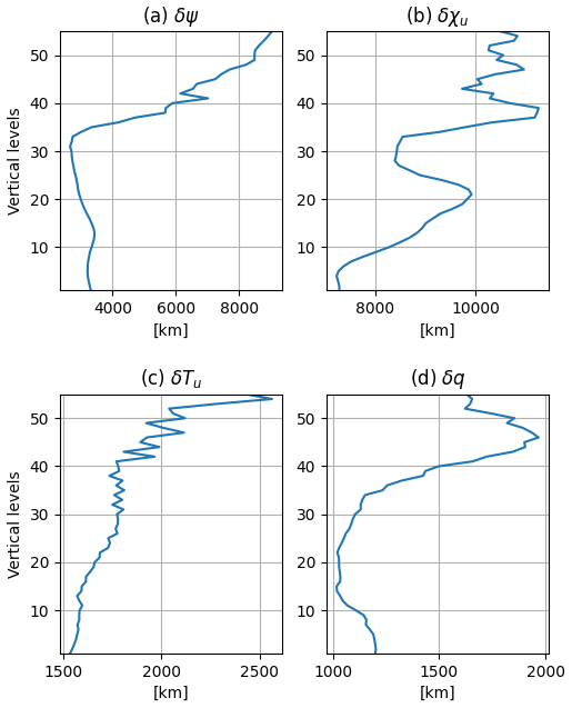
Figure 5Horizontally averaged horizontal correlation lengths [km] for (a) δψ, (b) δχu, (c) δTu, and (d) δq. The horizontally averaged length for δps,u is 3702.3 km.

Figure 6Horizontally averaged vertical correlation lengths [km] for (a) δψ, (b) δχu, (c) δTu, and (d) δq.
Figures 5 and 6 show the vertical profiles of horizontally averaged horizontal and vertical correlation lengths, respectively. The horizontal correlation lengths generally increase with height in the stratosphere and are nearly constant in the troposphere, though δχu has substantial variations in horizontal length scale throughout the profile. The horizontal correlation lengths for δψ and δχu are larger than those for δTu and δq, while the horizontal correlation length for δps,u is roughly 3700 km, much larger than the horizontal correlation lengths for δTu and δq near the surface. The vertical correlation lengths have minima near the surface for all variables and then increase with height toward a peak near the model top. The vertical correlation lengths for δψ and δχu are again larger than those for δTu and δq.
3.4 Additional tuning
The parameters shown in the previous section are the raw statistics from the BUMP training applications. We have applied two additional modifications to these raw statistics. Without these modifications, the resulting static B performs poorly in 3D-Var and is unable to improve on 3DEnVar in hybrid applications (not shown).
First, the background error standard deviation for all variables (Σ) is scaled by a factor of . While the cycling interval shown later in this study is 6 h, which is typical, the forecast differences used in the training reflect forecast-error evolution over 24 h. Thus, it is reasonable to scale the diagnosed background error standard deviation to match the error growth for a 6 h interval. Here, we choose the single scaling factor of for all variables, based on a limited set of sensitivity tests of cycling experiments with different scaling factors.
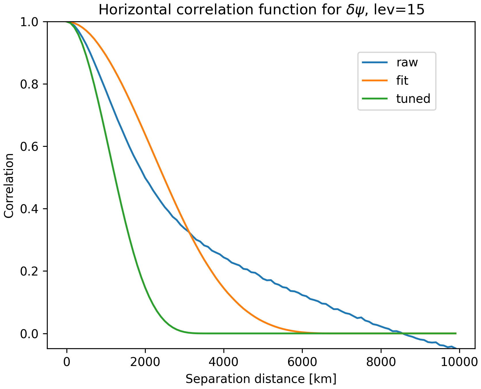
Figure 7The isotropic correlation function for δψ on the 15th model level, based on the sample of forecast differences (blue). Also shown are the correlation function assumed in BUMP (orange) using the length scale that gives the best fit to the sample-derived correlation, as well as the tuned correlation function (green).
We also reduce the diagnosed horizontal correlation lengths for δψ and δχu by half. Figure 7 shows the raw horizontal correlation function for δψ on model level 15 together with the best-fit correlation function, which is diagnosed by BUMP by adjusting the length scale of the fifth-order, compactly supported function from Gaspari and Cohn (1999). There is a clear discrepancy between the sample correlation function and that assumed in BUMP – the raw correlation decreases more rapidly for small separations and has larger correlations at large separations. The implied velocity variance in the modeled covariance (Eq. 2) is proportional to the second derivative at the origin of the δψ (and δχ) correlation (Lorenc, 1981; Daley, 1985). That is, δψ correlations that more strongly peak at the origin will produce larger velocity variance even if the δψ variance is fixed. Thus, the modeled covariances greatly underestimate the velocity variance relative to the statistics of the original training data. Reducing the horizontal correlation length for δψ and δχu by a factor of 2 increases the second derivative of their correlation, and therefore the velocity variance, by a factor of 4, leading to a better fit to the velocity variance in the training data. Ideally, the mismatch between the assumed correlation structure and that of the training data would be addressed by a more flexible correlation model in BUMP. A capability for this is now available, and we hope to report on its use in the future. In other systems, the necessary flexibility has been achieved using sums of recursive filters with different length scales (Wu et al., 2002; Kleist et al., 2009) or modeling the correlations in spectral space (Parrish and Derber, 1992; Lorenc et al., 2000).
To explore the structure of diagnosed and tuned multivariate B, two sets of a single-observation test were performed; one for assimilating a single zonal-wind observation with 1 m s−1 innovation and 1 m s−1 observation-error standard deviation and the other for assimilating a single temperature observation with 1 K innovation and 1 K observation-error standard deviation. Both single observations are placed at (40.4113° N, 38.68° W) and at roughly 800 hPa, a location that corresponds to one of the MPAS cell centers and vertical level 15.
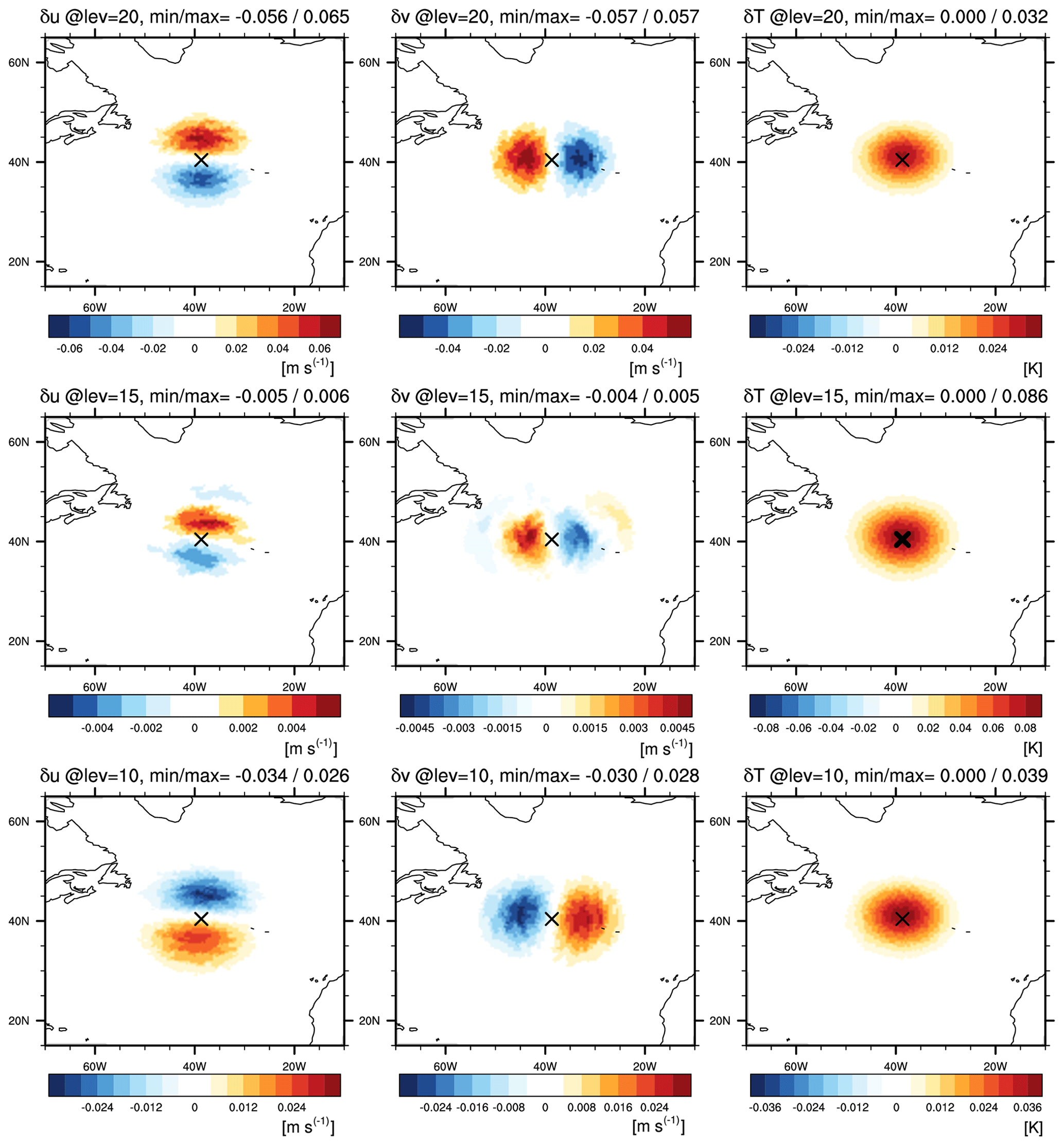
Figure 8Analysis increments for the (left column) zonal component of v [m s−1], (center column) meridional component of v [m s−1], and (right column) T [K] on model level (upper row) 20, (middle row) 15, and (lower row) 10, from a single temperature observation with 1 K innovation and 1 K observation-error standard deviation, located at (40.41° N, 38.68° W) on model level 15 with a marker ×.
Figure 8 shows the analysis increments from the single temperature observation, for the zonal and meridional components of v (left and center columns, respectively) and for T (right column), on the three different vertical levels (10, 15, and 20, shown in the bottom, middle, and top rows). The T increments have a horizontally isotropic structure with maximum values at level 15, where the observation is located. The wind increments are, to a first approximation, linked to the T increment through the thermal-wind relation: cyclonic circulation is introduced on level 10, below the maximum temperature increment, and an anti-cyclonic circulation appears above, on level 20. This reflects the approximate geostrophic and hydrostatic relations captured by K2 and is consistent with Parrish and Derber (1992) (their Fig. 2), which uses the linear balance equation between mass and momentum variables.
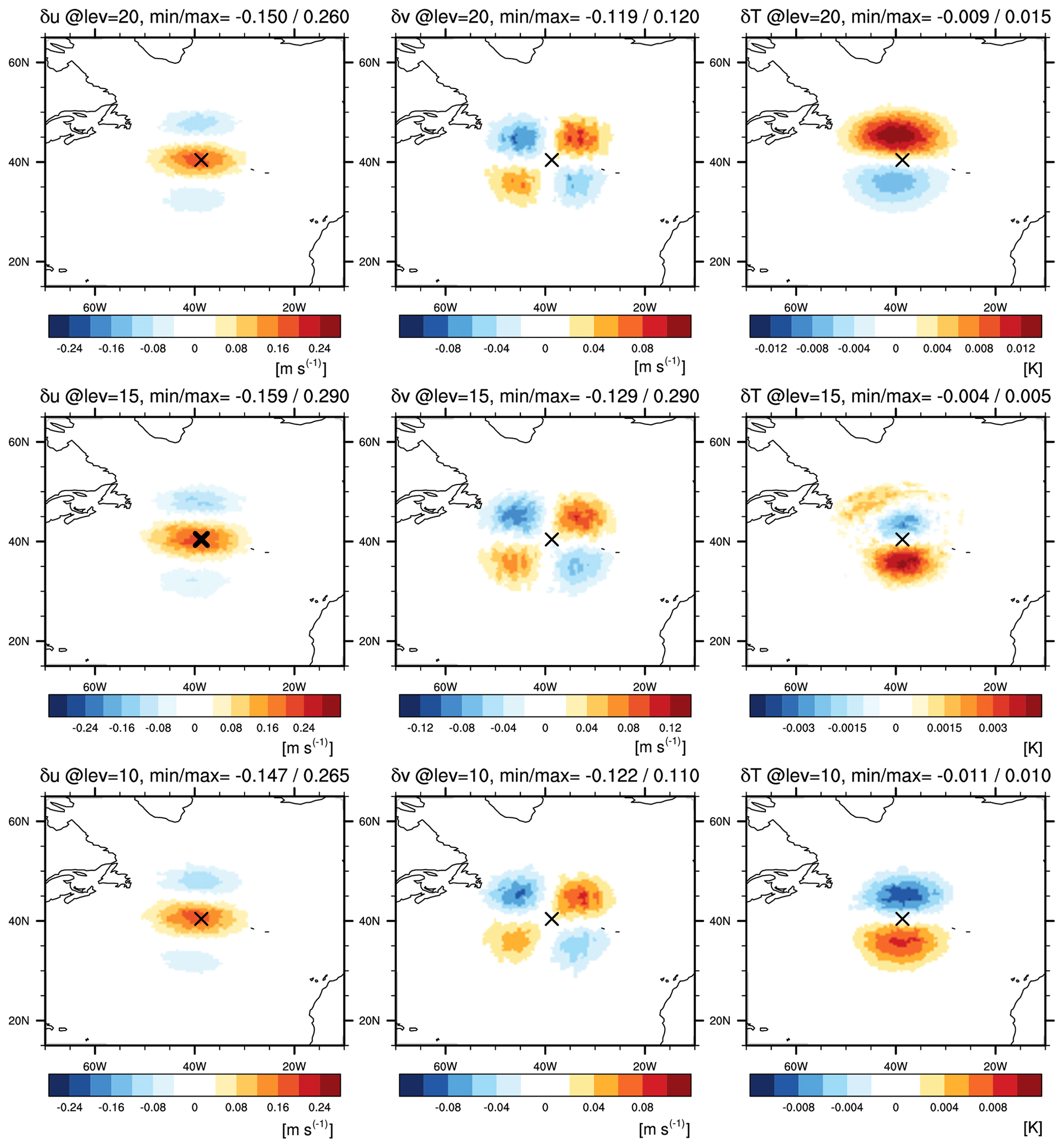
Figure 9Same as Fig. 8, except from a single zonal-wind observation with 1 m s−1 innovation and 1 m s−1 observation-error standard deviation, located at (40.41° N, 38.68° W) on model level 15 with a marker ×.
Similarly, Fig. 9 shows the analysis increments from the single zonal-wind observation. The positive zonal-wind increment is maximized at the observation location on the 15th model level. To the north and south of the observation location, negative zonal-wind increments are introduced, which – together with the increments of meridional winds – represent a cyclonic circulation to the north of the observation and an anti-cyclonic circulation to the south. Temperature increments are negative below the cyclonic circulation (i.e., on level 10) and positive above (on level 20) and vice versa for the anti-cyclonic circulation. The structure of the increments again reflects thermal-wind balance, and in this case is consistent with Wu et al. (2002) (their Fig. 9) or Kleist et al. (2009) (their Fig. 3).
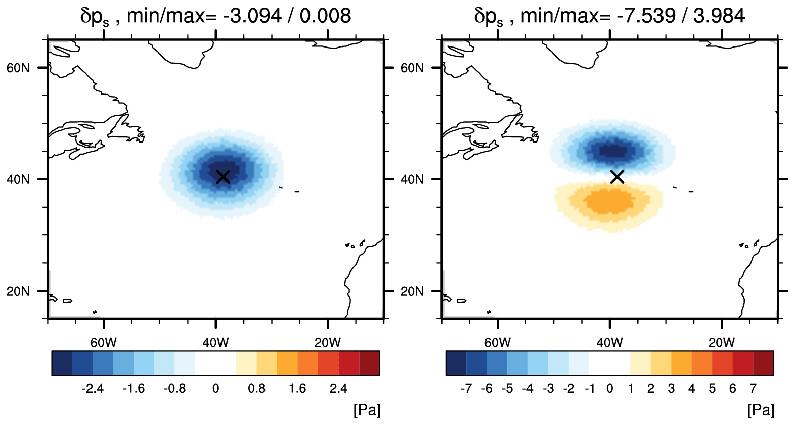
Figure 10Analysis increments for ps [Pa] (left) from a single temperature observation with 1 K innovation and 1 K observation-error standard deviation and (right) from a single zonal-wind observation with 1 m s−1 innovation and 1 m s−1 observation-error standard deviation. The observation location is marked with ×.
Figure 10 shows the surface pressure increments from two single-observation tests. When the single temperature observation is assimilated, cyclonic circulation is introduced into the lower troposphere. The negative surface pressure increment is approximately geostrophically related to this cyclonic circulation. When the single zonal-wind observation is assimilated, the zonal-wind increments extend throughout the troposphere, including to the surface. The dipole of positive and negative surface pressure increments, south and north, respectively, of the observation location, is geostrophically related to the increment of the surface wind.
5.1 Experimental design and assimilated observations
For further evaluation of the multivariate static B for JEDI-MPAS, three sets of 1-month (15 April–14 May 2018) cycling experiments were performed on NCAR's high-performance computing system, Cheyenne. As a reference experiment, the “3DEnVar” experiment was performed using the pure ensemble covariances, as in Liu et al. (2022). At each cycle, a 20-member ensemble of 6 h MPAS forecasts was made using initial conditions from the Global Ensemble Forecast System (GEFS; Zhou et al., 2017). Covariance localization was applied to the ensemble covariances via BUMP's generic localization scheme, using globally constant localization scales of 1200 km horizontally and 6 km vertically. To demonstrate the static covariances, the “3D-Var” experiment was performed with the static B formulated and tuned as described in the preceding sections. Lastly, the “Hybrid-3DEnVar” experiment was performed using a hybrid covariance given by a weighted sum of static and ensemble B (Hamill and Snyder, 2000). Here, we choose a weight of 0.5 for each component, similarly to Wang et al. (2013), Clayton et al. (2013), and Kuhl et al. (2013). This final experiment evaluates the effectiveness of our static B for hybrid applications. In all three experiments, the same global MPAS quasi-uniform 60 km mesh is used both for analysis and background fields and for analysis increment. For the minimization, two outer loops are used, with 60 inner iterations for each outer loop.
The observation files are converted from GSI's ncdiag files, which contain the observation location, observation value, observation error, GSI's quality control, and satellite bias correction information. The observation quality control basically follows the GSI's quality control (called “PREQC”), and the background innovation check is added, which filters out the observation when the absolute value of observation departure is larger than 3 times the given observation error. In all three experiments, the surface pressure, radiosondes (wind, temperature or virtual temperature, and specific humidity), aircraft (wind, temperature, specific humidity), atmospheric motion vectors, Global Navigation Satellite System Radio Occultation (GNSS RO) refractivity, and clear-sky Advanced Microwave Sounding Unit-A (AMSU-A) radiances from NOAA-15, NOAA-18, and NOAA-19; MetOp-A and MetOp-B; and Aqua satellites are assimilated. The AMSU-A radiances are bias-corrected from GSI's information and pre-thinned with a 145 km mesh.
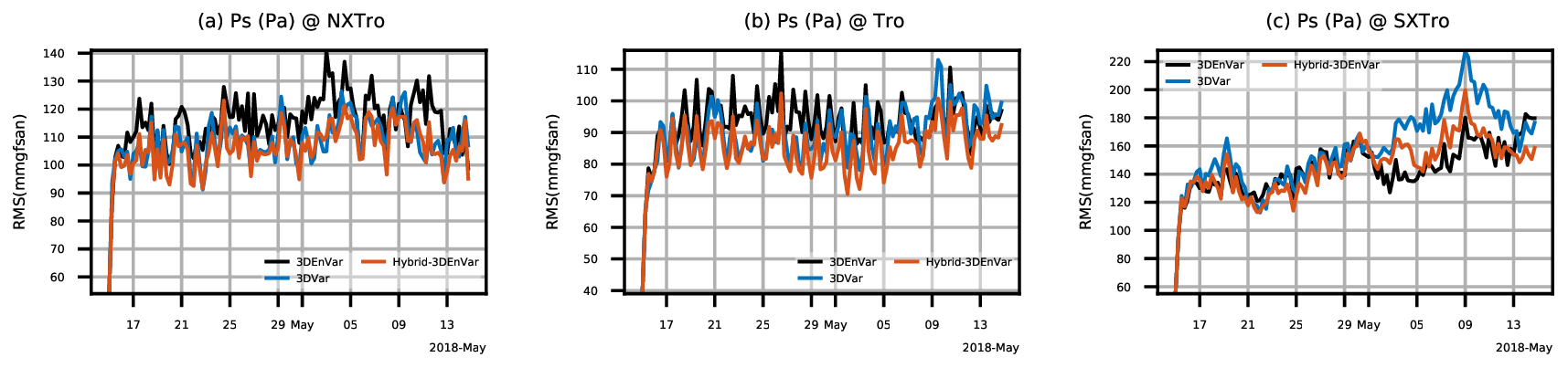
Figure 11Time series (00:00 UTC, 15 April, to 18:00 UTC, 14 May 2018) of background RMSEs for ps verified with GFS analysis over (a) northern extratropical (30–90° N; NXTro), (b) tropical (30° S–30° N; Tro), and (c) southern extratropical (30–90° S; SXTro) regions.
5.2 Results
Figure 11 shows the time series of background RMSEs for surface pressure during the cycling period. The RMSEs are calculated with respect to GFS analysis at the valid time as a reference. For surface pressure, 3D-Var gives somewhat smaller RMSEs compared to the 3DEnVar experiment, except for the southern extratropical region. Hybrid-3DEnVar gives smaller RMSEs compared to 3D-Var. Figure 12 shows the vertical profiles of relative RMSE changes for background fields during the cycling period, with the RMSE of 3DEnVar as reference. The confidence intervals with 95 % significant level are also shown as error bars, from a bootstrap resampling method with a resampling size of 10 000. Compared to 3DEnVar, the 3D-Var experiment shows some degradation in the troposphere and some improvement in the stratosphere in general. Hybrid-3DEnVar shows overall improvement over both 3DEnVar and 3D-Var experiments and throughout levels in both the troposphere and the stratosphere.
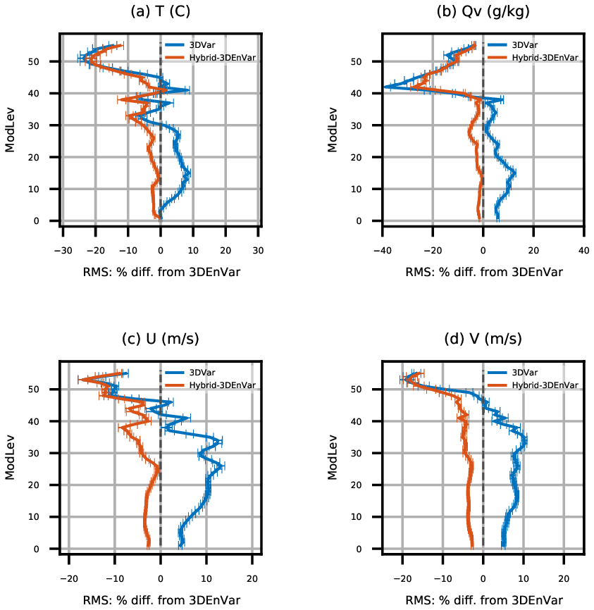
Figure 12Vertical profiles of relative background RMSE changes (with respect to GFS analysis) for (a) T, (b) Qv, (c) zonal wind, and (d) meridional wind, compared to the 3DEnVar experiment. Statistics are aggregated for the period from 00:00 UTC, 18 April, to 18:00 UTC, 14 May 2018, with 95 % confidence intervals.
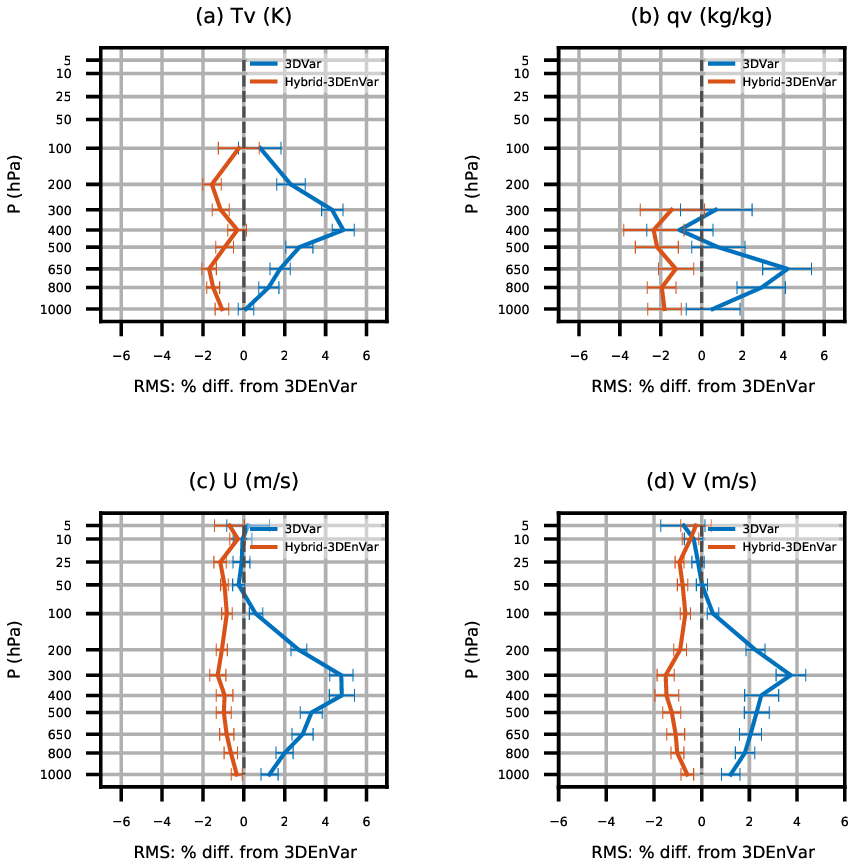
Figure 13Vertical distribution of relative rms changes of observation minus background, or first-guess departure, for the (a) virtual temperature Tv, (b) specific humidity (c) zonal wind, and (d) meridional wind of radiosonde observations. Statistics are aggregated for the period from 00:00 UTC, 18 April, to 18:00 UTC, 14 May 2018, with 95 % confidence intervals.
Figure 13 shows the observation space verification for radiosondes. The relative changes of the root mean square (rms) first-guess departure (OMB, observation minus background) are mostly consistent with the model space verification in Fig. 12. Compared to the RMSEs of 3DEnVar, the RMSEs of Hybrid-3DEnVar are significantly improved, except for temperature observation. The RMSEs of 3D-Var are degraded by ∼5 %. In the observation space verification for AMSU-A radiance observations (not shown), which assimilates the channels sensitive to the atmospheric temperature profile, Hybrid-3DEnVar shows neutral to slightly improved impact in the RMSEs for channels 5 and 6. For channels 7, 8, and 9, both 3D-Var and Hybrid-3DEnVar show significant improvement over 3DEnVar. Larger improvement is shown over both high latitudes. This is consistent with the large temperature RMSE reduction in the model space verification (Fig. 12a).
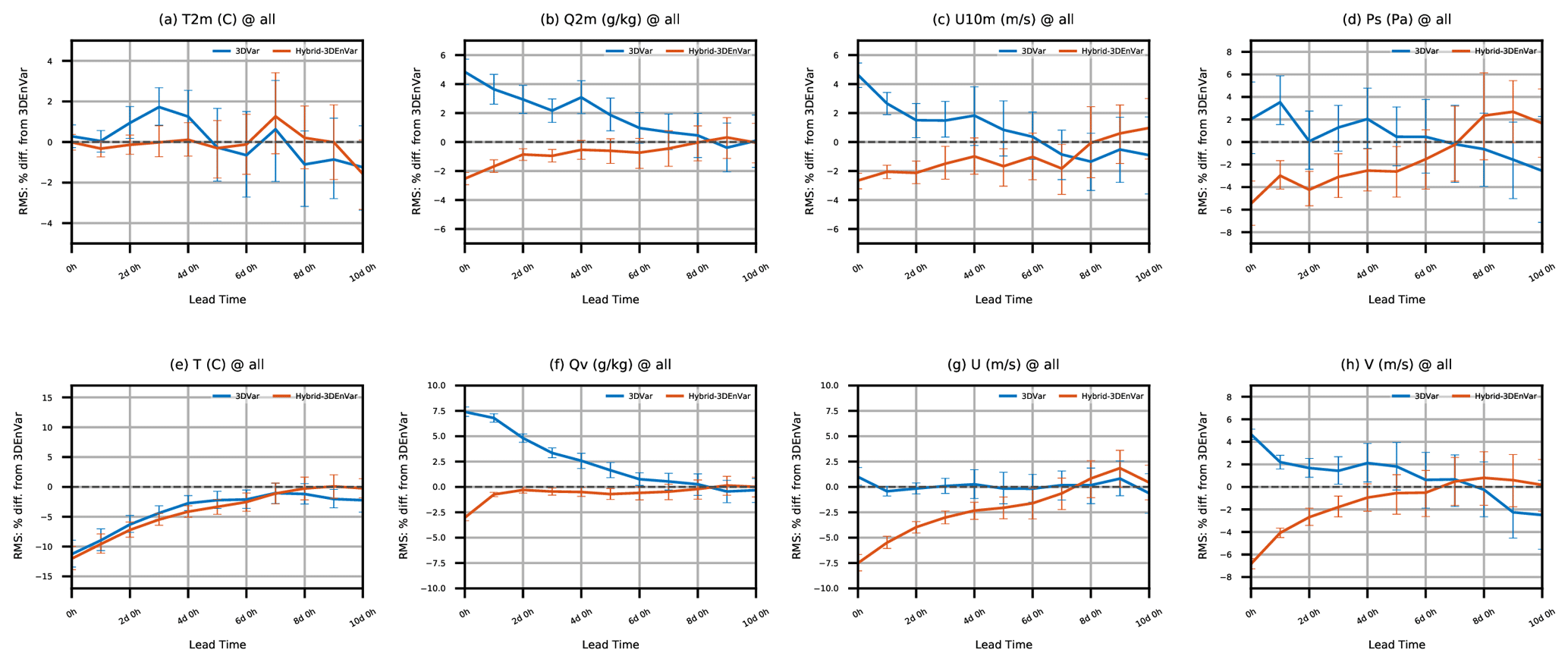
Figure 14Relative RMSE changes as a function of forecast lead time for (a–d) near-surface and (e–h) three-dimensional variables, compared to the 3DEnVar experiment. Shown are (a) T at 2 m, (b) q at 2 m, (c) zonal wind at 10 m, (d) ps, (e) T, (f) Qv, (g) zonal wind, and (h) meridional wind. Statistics are aggregated over 27 extended forecasts with 95 % confidence intervals.
Additional 10 d extended forecasts were conducted at each 00:00 UTC initialization time to evaluate the impact of analysis on the longer forecast lengths. The changes in RMSE for 3D-Var and Hybrid-3DEnVar relative to 3DEnVar are shown in Fig. 14. At short forecast lead times, the relative RMSEs look similar to the relative RMSEs for the 6 h background forecasts shown in Figs. 11 and 12. It is notable that the larger water vapor mixing ratio (Qv) RMSE for 3D-Var lasts until 6 d forecasts (Fig. 14f). This might be because the moisture variable is univariate in the current B design (Sect. 3.1), while the moisture analysis in 3DEnVar or Hybrid-3DEnVar can be done through the multivariate ensemble covariances. The benefit of hybrid background error covariance can be found for up to 5 d lead times for surface pressure, temperature, and zonal- and meridional-wind fields. The benefit of hybrid covariance is only kept for ∼2 d lead times for humidity fields.
This study has described the multivariate static background error covariances for JEDI-MPAS 3D-Var. Similarly to Liu et al. (2022), JEDI-MPAS 3D-Var utilizes generic JEDI components through interfaces that are specific to MPAS.
The formulation of the JEDI-MPAS static B generally follows Wu et al. (2002) but with the novel use of BUMP for multiple elements of the covariance model. Two linear variable transforms represent the multivariate relationship. One transform is a variable change from stream function ψ and velocity potential χ to v, which directly operates on the MPAS native mesh. The other transform, which uses the BUMP driver VBAL from JEDI's SABER repository, is based on linear regression over vertical columns of increments in other variables against increments in ψ. The full multivariate covariances are then given by these linear transforms (and their adjoints) applied to a univariate covariance. The univariate correlation matrix employs BUMP–NICAS, which efficiently computes the three-dimensional convolution of an input vector with a specified spatial correlation function on an optimally subsampled mesh and then interpolates back to the full MPAS mesh.
For the experiments presented here, we estimated various parameters in the covariance model from a training data set of 366 differences between 48 and 24 h forecasts on the 60 km MPAS mesh. In general, the regression coefficients capture the linear, approximately geostrophic balance between mass and momentum variables that holds outside the tropics. While the error standard deviations for ψ and χu become larger at higher vertical levels, up to a peak near the tropopause, the error standard deviations for Tu and q are larger in the middle to lower troposphere. The horizontal and vertical correlation lengths for errors in ψ and χu are, in general, larger than those for errors in Tu and q. We also made two modifications to the parameters objectively estimated by BUMP. The error standard deviation is scaled by a factor of to match the 24 h time differences (i.e., 48 h forecast and 24 forecast pairs) in the training samples to the typical 6 h DA cycling interval. In addition, the horizontal correlation lengths for increments of ψ and χu are reduced by half to compensate for the discrepancy between the raw correlation structure from the training data set and the correlation function assumed in BUMP, which has much less curvature at small separations.
We evaluated the JEDI-MPAS static B in cycling data assimilation experiments extending over a month and assimilating observations from a significant fraction of the global observing network, including GNSS RO, AMSU-A, and conventional observations. The 3D-Var system using this static B generally performs close to, but worse than, EnVar using pure ensemble covariances as in Liu et al. (2022), while using a hybrid background covariance that is a weighted sum of the static B and ensemble covariances improves significantly on both 3D-Var and EnVar. Neither of these results is novel, as numerous studies have shown the advantage of EnVar over 3D-Var and of the hybrid algorithm over EnVar, but they do demonstrate clearly the effectiveness of the static B.
The static background covariances presented here are an initial implementation, with plenty of room for further refinements. Two extensions that are already underway are training the covariance model based on an ensemble from JEDI-MPAS, such as that provided by the EDA of Guerrette et al. (2023), and including hydrometeor increments, which will be especially important for all-sky assimilation of radiances. There are also BUMP capabilities that we have yet to exercise, including more general correlation functions that should remove the need for manual retuning of correlation lengths diagnosed by BUMP and joint estimation of hybridization and localization coefficients (Ménétrier and Auligné, 2015). In the current B design, the moisture variable is univariate, which may limit the performance of moisture analysis even with Hybrid-3DEnVar configuration. To this end, we will explore more sophisticated moisture variables, such as pseudo-relative humidity (Dee and da Silva, 2003) or normalized relative humidity (Hólm et al., 2002).
To compute horizontal velocity v from ψ and χ on the MPAS mesh, we rely on the fact that the irrotational component of velocity is given by (minus) the gradient of χ, while the nondivergent component of velocity is given by the cross-product of the vertical unit vector and the gradient of ψ. The edge-normal component of velocity u on the MPAS mesh is oriented parallel to the segment connecting the centers of adjacent cells and, naturally, normal to the edge itself. The natural finite difference relation is then
where, in an abuse of our previous notation, δc is the difference operator between the centers of the mesh cells adjoining the edge and δv is the difference operator between the cell vertices at either end of the edge.
Implementing Eq. (A1) is straightforward given the MPAS mesh conventions and the mesh information in MPAS initialization files (MPAS Mesh Specification, 2015). The difference operators are defined as
where Δc is the distance between cell centers sharing the edge and Δv is the distance between vertices on the edge. The ordering of the cells and vertices is such that this formula will give the correct signs for the velocities on the MPAS mesh. For a given edge in the files, the lengths Δc and Δv are in the variables dcEdge(edge) and dvEdge(edge), respectively. The cells sharing an edge are cellsOnEdge(2,edge) and cellsOnEdge(1,edge), and the vertices are verticesOnEdge(2,edge) and verticesOnEdge(1,edge).
Although Eqs. (A1) and (A2) use the full variables (i.e., ψ and χ), they are also applicable to the incremental variables (i.e., δψ and δχ) because of their linear form. The computation begins with δψ and δχ at the cell centers. Values of δψ at the cell vertices are computed by interpolating δψ from the centers of the three cells containing each vertex, before applying Eq. (A1). MPAS provides a utility that employs radial basis functions to reconstruct the vector wind at a cell center from δu on the edges of the cell (following Bonaventura et al., 2011), which provides the final δv. Because these three steps involve a different subset of the MPAS mesh (i.e., cells, vertices, and edges), a halo exchange routine from MPAS is required and called between each step. We have also implemented the adjoint operator of the halo exchange, which is needed when applying .
JEDI-MPAS 2.0.0-beta has been publicly released on GitHub, accessible in the release/2.0.0-beta branch of mpas-bundle (https://github.com/JCSDA/mpas-bundle/tree/release/2.0.0-beta, last access: 6 May 2024). It is also available from Zenodo at https://doi.org/10.5281/zenodo.7630054 (Joint Center For Satellite Data Assimilation and National Center For Atmospheric Research, 2022). Global Forecast System analysis data were downloaded from the NCAR Research Data Archive: https://doi.org/10.5065/D65D8PWK (last access: 1 June 2023; National Centers for Environmental Prediction/National Weather Service/NOAA/U.S. Department of Commerce, 2015). Global Ensemble Forecast System ensemble analysis data were downloaded from https://www.ncei.noaa.gov/products/weather-climate-models/global-ensemble-forecast (last access: 1 June 2023; NOAA, 2023). Conventional and satellite observations assimilated were downloaded from https://doi.org/10.5065/Z83F-N512 (last access: 1 June 2023; National Centers for Environmental Prediction/National Weather Service/NOAA/U.S. Department of Commerce, 2008) and https://doi.org/10.5065/DWYZ-Q852 (last access: 1 June 2023; National Centers for Environmental Prediction/National Weather Service/NOAA/U.S. Department of Commerce, 2009).
BJJ designed, conducted, and analyzed all experiments and wrote the manuscript. BM gave feedback on configuring the BUMP drivers and developed the necessary component in BUMP. CS and ZL contributed the design of multivariate covariance formulation and analysis of experimental results. WCS provided the discretized equation for wind transform shown in the Appendix. All co-authors contributed to the development of the JEDI-MPAS source code and experimental workflow, preparation of externally sourced data, design of experiments, and preparation of the manuscript.
The contact author has declared that none of the authors has any competing interests.
Publisher's note: Copernicus Publications remains neutral with regard to jurisdictional claims made in the text, published maps, institutional affiliations, or any other geographical representation in this paper. While Copernicus Publications makes every effort to include appropriate place names, the final responsibility lies with the authors.
The National Center for Atmospheric Research is sponsored by the National Science Foundation of the United States. We would like to acknowledge high-performance computing support from Cheyenne (https://doi.org/10.5065/D6RX99HX; NCAR, 2023) provided by NCAR's Computational and Information Systems Laboratory, sponsored by the National Science Foundation. Michael Duda in the Mesoscale and Microscale Meteorology (MMM) laboratory provided guidance on modifying MPAS-A for JEDI-MPAS applications.
This research has been supported by the United States Air Force (grant no. NA21OAR4310383).
This paper was edited by Shu-Chih Yang and reviewed by Ting-Chi Wu and one anonymous referee.
Andersson, E., Haseler, J., Undén, P., Courtier, P., Kelly, G., Vasiljevic, D., Brankovic, C., Gaffard, C., Hollingsworth, A., Jakob, C., Janssen, P., Klinker, E., Lanzinger, A., Miller, M., Rabier, F., Simmons, A., Strauss, B., Viterbo, P., Cardinali, C., and Thépaut, J.-N.: The ECMWF implementation of three-dimensional variational assimilation (3D-Var). III: Experimental results, Q. J. Roy. Meteor. Soc., 124, 1831–1860, https://doi.org/10.1002/qj.49712455004, 1998. a
Bannister, R. N.: A review of forecast error covariance statistics in atmospheric variational data assimilation. II: Modelling the forecast error covariance statistics, Q. J. Roy. Meteor. Soc., 134, 1971–1996, https://doi.org/10.1002/qj.340, 2008. a
Barker, D., Huang, X.-Y., Liu, Z., Auligné, T., Zhang, X., Rugg, S., Ajjaji, R., Bourgeois, A., Bray, J., Chen, Y., Demirtas, M., Guo, Y.-R., Henderson, T., Huang, W., Lin, H.-C., Michalakes, J., Rizvi, S., and Zhang, X.: The Weather Research and Forecasting Model's Community Variational/Ensemble Data Assimilation System: WRFDA, B. Am. Meteorol. Soc., 93, 831–843, https://doi.org/10.1175/BAMS-D-11-00167.1, 2012. a, b
Bonaventura, L., Iske, A., and Miglio, E.: Kernel-based vector field reconstruction in computational fluid dynamic models, Int. J. Numer. Meth. Fluids, 66, 714–729, https://doi.org/10.1002/fld.2279, 2011. a
Buehner, M.: Ensemble-derived stationary and flow-dependent background-error covariances: Evaluation in a quasi-operational NWP setting, Q. J. Roy. Meteor. Soc., 131, 1013–1043, https://doi.org/10.1256/qj.04.15, 2005. a
Buehner, M., Morneau, J., and Charette, C.: Four-dimensional ensemble-variational data assimilation for global deterministic weather prediction, Nonlin. Processes Geophys., 20, 669–682, https://doi.org/10.5194/npg-20-669-2013, 2013. a
Clayton, A. M., Lorenc, A. C., and Barker, D. M.: Operational implementation of a hybrid ensemble/4D-Var global data assimilation system at the Met Office, Q. J. Roy. Meteor. Soc., 139, 1445–1461, https://doi.org/10.1002/qj.2054, 2013. a, b
Daley, R.: The Analysis of Synoptic Scale Divergence by a Statistical Interpolation Procedure, Mon. Weather Rev., 113, 1066–1080, https://doi.org/10.1175/1520-0493(1985)113<1066:TAOSSD>2.0.CO;2, 1985. a
Dee, D. P. and da Silva, A. M.: The Choice of Variable for Atmospheric Moisture Analysis, Mon. Weather Rev., 131, 155–171, https://doi.org/10.1175/1520-0493(2003)131<0155:TCOVFA>2.0.CO;2, 2003. a
Derber, J. and Bouttier, F.: A reformulation of the background error covariance in the ECMWF global data assimilation system, Tellus A, 51, 195–221, https://doi.org/10.3402/tellusa.v51i2.12316, 1999. a, b, c
Derber, J. and Rosati, A.: A Global Oceanic Data Assimilation System, J. Phys. Oceanogr., 19, 1333–1347, https://doi.org/10.1175/1520-0485(1989)019<1333:AGODAS>2.0.CO;2, 1989. a
Gaspari, G. and Cohn, S. E.: Construction of correlation functions in two and three dimensions, Q. J. Roy. Meteor. Soc., 125, 723–757, https://doi.org/10.1002/qj.49712555417, 1999. a, b, c
Gauthier, P., Charette, C., Fillion, L., Koclas, P., and Laroche, S.: Implementation of a 3D variational data assimilation system at the Canadian Meteorological Centre. Part I: The global analysis, Atmosphere-Ocean, 37, 103–156, https://doi.org/10.1080/07055900.1999.9649623, 1999. a
Golub, G. H. and Ye, Q.: Inexact Preconditioned Conjugate Gradient Method with Inner-Outer Iteration, SIAM J. Sci. Comput., 21, 1305–1320, 1999. a
Guerrette, J. J., Liu, Z., Snyder, C., Jung, B.-J., Schwartz, C. S., Ban, J., Vahl, S., Wu, Y., Baños, I. H., Yu, Y. G., Ha, S., Trémolet, Y., Auligné, T., Gas, C., Ménétrier, B., Shlyaeva, A., Miesch, M., Herbener, S., Liu, E., Holdaway, D., and Johnson, B. T.: Data assimilation for the Model for Prediction Across Scales – Atmosphere with the Joint Effort for Data assimilation Integration (JEDI-MPAS 2.0.0-beta): ensemble of 3D ensemble-variational (En-3DEnVar) assimilations, Geosci. Model Dev., 16, 7123–7142, https://doi.org/10.5194/gmd-16-7123-2023, 2023. a, b, c
Hamill, T. M. and Snyder, C.: A Hybrid Ensemble Kalman Filter–3D Variational Analysis Scheme, Mon. Weather Rev., 128, 2905–2919, https://doi.org/10.1175/1520-0493(2000)128<2905:AHEKFV>2.0.CO;2, 2000. a, b
Hólm, E., Andersson, E., Beljaars, A., Lopez, P., Mahfouf, J.-F., Simmons, A., and Thépaut, J.-N.: Assimilation and Modelling of the Hydrological Cycle: ECMWF's Status and Plans, ECMWF Technical Memoranda, 55, https://doi.org/10.21957/kry8prwuq, 2002. a
Joint Center For Satellite Data Assimilation and National Center For Atmospheric Research: JEDI-MPAS Data Assimilation System v2.0.0-beta, Zenodo [code], https://doi.org/10.5281/ZENODO.7630054, 2022. a
Kleist, D. T., Parrish, D. F., Derber, J. C., Treadon, R., Wu, W.-S., and Lord, S.: Introduction of the GSI into the NCEP Global Data Assimilation System, Weather Forecast., 24, 1691–1705, https://doi.org/10.1175/2009WAF2222201.1, 2009. a, b
Kuhl, D. D., Rosmond, T. E., Bishop, C. H., McLay, J., and Baker, N. L.: Comparison of Hybrid Ensemble/4DVar and 4DVar within the NAVDAS-AR Data Assimilation Framework, Mon. Weather Rev., 141, 2740–2758, https://doi.org/10.1175/MWR-D-12-00182.1, 2013. a, b
Liu, Z., Snyder, C., Guerrette, J. J., Jung, B.-J., Ban, J., Vahl, S., Wu, Y., Trémolet, Y., Auligné, T., Ménétrier, B., Shlyaeva, A., Herbener, S., Liu, E., Holdaway, D., and Johnson, B. T.: Data assimilation for the Model for Prediction Across Scales – Atmosphere with the Joint Effort for Data assimilation Integration (JEDI-MPAS 1.0.0): EnVar implementation and evaluation, Geosci. Model Dev., 15, 7859–7878, https://doi.org/10.5194/gmd-15-7859-2022, 2022. a, b, c, d, e, f, g, h, i, j, k
Lorenc, A. C.: A Global Three-Dimensional Multivariate Statistical Interpolation Scheme, Mon. Weather Rev., 109, 701–721, https://doi.org/10.1175/1520-0493(1981)109<0701:AGTDMS>2.0.CO;2, 1981. a
Lorenc, A. C.: The potential of the ensemble Kalman filter for NWP – a comparison with 4D-Var, Q. J. Roy. Meteor. Soc., 129, 3183–3203, https://doi.org/10.1256/qj.02.132, 2003. a
Lorenc, A. C., Ballard, S. P., Bell, R. S., Ingleby, N. B., Andrews, P. L. F., Barker, D. M., Bray, J. R., Clayton, A. M., Dalby, T., Li, D., Payne, T. J., and Saunders, F. W.: The Met. Office global three-dimensional variational data assimilation scheme, Q. J. Roy. Meteor. Soc., 126, 2991–3012, https://doi.org/10.1002/qj.49712657002, 2000. a, b
Ménétrier, B.: Normalized Interpolated Convolution from an Adaptive Subgrid documentation, https://github.com/benjaminmenetrier/nicas_doc/blob/master/nicas_doc.pdf (last access: 6 May 2024), 2020. a, b
Ménétrier, B. and Auligné, T.: Optimized Localization and Hybridization to Filter Ensemble-Based Covariances, Mon. Weather Rev., 143, 3931–3947, https://doi.org/10.1175/MWR-D-15-0057.1, 2015. a
MPAS Mesh Specification: MPAS Mesh Specification, https://mpas-dev.github.io/files/documents/MPAS-MeshSpec.pdf (last access: 19 May 2023), 2015. a
National Centers for Environmental Prediction/National Weather Service/NOAA/U.S. Department of Commerce: NCEP ADP Global Upper Air and Surface Weather Observations (PREPBUFR format), Research Data Archive at the National Center for Atmospheric Research, Computational and Information Systems Laboratory [data set], https://doi.org/10.5065/Z83F-N512 (last access: 1 June 2023), 2008, updated daily. a
National Centers for Environmental Prediction/National Weather Service/NOAA/U.S. Department of Commerce: NCEP GDAS Satellite Data 2004–continuing, Research Data Archive at the National Center for Atmospheric Research, Computational and Information Systems Laboratory [data set], https://doi.org/10.5065/DWYZ-Q852 (last access: 1 June 2023), 2009, updated daily. a
National Centers for Environmental Prediction/National Weather Service/NOAA/U.S. Department of Commerce: NCEP GFS 0.25 Degree Global Forecast Grids Historical Archive, Research Data Archive at the National Center for Atmospheric Research, Computational and Information Systems Laboratory [data set], https://doi.org/10.5065/D65D8PWK (last access: 1 June 2023), 2015, updated daily. a
NCAR: HPE SGI ICE XA – Cheyenne, https://doi.org/10.5065/D6RX99HX, 2023. a
NCL: The NCAR Command Language (Version 6.6.2), NCL [software], https://doi.org/10.5065/D6WD3XH5, 2019. a
NOAA: Global Ensemble Forecast System (GEFS), NOAA [data set], https://www.ncei.noaa.gov/products/weather-climate-models/global-ensemble-forecast, last access: 1 June 2023. a
Parrish, D. F. and Derber, J. C.: The National Meteorological Center's Spectral Statistical-Interpolation Analysis System, Mon. Weather Rev., 120, 1747–1763, https://doi.org/10.1175/1520-0493(1992)120<1747:TNMCSS>2.0.CO;2, 1992. a, b, c
Rabier, F., Järvinen, H., Klinker, E., Mahfouf, J.-F., and Simmons, A.: The ECMWF operational implementation of four-dimensional variational assimilation. I: Experimental results with simplified physics, Q. J. Roy. Meteor. Soc., 126, 1143–1170, https://doi.org/10.1002/qj.49712656415, 2000. a
Rawlins, F., Ballard, S. P., Bovis, K. J., Clayton, A. M., Li, D., Inverarity, G. W., Lorenc, A. C., and Payne, T. J.: The Met Office global four-dimensional variational data assimilation scheme, Q. J. Roy. Meteor. Soc., 133, 347–362, https://doi.org/10.1002/qj.32, 2007. a
Skamarock, W. C., Klemp, J. B., Duda, M. G., Fowler, L. D., Park, S.-H., and Ringler, T. D.: A Multiscale Nonhydrostatic Atmospheric Model Using Centroidal Voronoi Tesselations and C-Grid Staggering, Mon. Weather Rev., 140, 3090–3105, https://doi.org/10.1175/mwr-d-11-00215.1, 2012. a, b
Trémolet, Y.: Joint Effort for Data Assimilation Integration (JEDI) Design and Structure, JCSDA Quarterly Newsletter, 66, 6–14, https://doi.org/10.25923/RB19-0Q26, 2020. a
Trémolet, Y. and Auligné, T.: The Joint Effort for Data Assimilation Integration (JEDI), JCSDA Quarterly Newsletter, 66, 1–5, https://doi.org/10.25923/RB19-0Q26, 2020. a
Wang, X., Barker, D. M., Snyder, C., and Hamill, T. M.: A hybrid ETKF–3DVAR data assimilation scheme for the WRF Model. Part II: Real observation experiments, Mon. Weather Rev., 136, 5132–5147, https://doi.org/10.1175/2008MWR2445.1, 2008. a
Wang, X., Parrish, D., Kleist, D., and Whitaker, J.: GSI 3DVar-Based Ensemble–Variational Hybrid Data Assimilation for NCEP Global Forecast System: Single-Resolution Experiments, Mon. Weather Rev., 141, 4098–4117, https://doi.org/10.1175/MWR-D-12-00141.1, 2013. a
Wu, W.-S., Purser, R. J., and Parrish, D. F.: Three-dimensional variational analysis with spatially inhomogeneous covariances, Mon. Weather Rev., 130, 2905–2916, https://doi.org/10.1175/1520-0493(2002)130<2905:TDVAWS>2.0.CO;2, 2002. a, b, c, d, e, f
Zhou, X., Zhu, Y., Hou, D., Luo, Y., Peng, J., and Wobus, R.: Performance of the New NCEP Global Ensemble Forecast System in a Parallel Experiment, Weather Forecast., 32, 1989–2004, https://doi.org/10.1175/WAF-D-17-0023.1, 2017. a
- Abstract
- Introduction
- JEDI-MPAS 3D-Var configuration
- Multivariate background error covariance
- Single-observation tests
- Cycling experiments
- Conclusions
- Appendix A: Diagnosing velocity from the stream function and velocity potential in MPAS
- Code and data availability
- Author contributions
- Competing interests
- Disclaimer
- Acknowledgements
- Financial support
- Review statement
- References