Balloon drift estimation and improved position estimates for radiosondes

When comparing model output with historical radiosonde observations, it is usually assumed that a radiosonde has risen exactly above its starting point and has not been displaced by wind. This changed only relatively recently with the availability of Global Navigation Satellite System (GNSS) receivers aboard radiosondes in the late 1990s, but even then the balloon trajectory data were often not transmitted, although this information was the basis for estimating the wind in the first place. Depending on the conditions and time of year, radiosondes can sometimes drift a few hundred kilometres, particularly at the middle latitudes during the winter months. The position errors can lead to non-negligible representation errors when the corresponding observations are assimilated.

This paper presents a methodology to compute changes in the balloon position during its vertical ascent, using only limited information, such as the vertical profile of wind contained in the historical observation reports. The sensitivity of the method to various parameters is investigated, such as the vertical resolution of the input data, the assumption about the vertical ascent speed of the balloon, and the departure of the surface of Earth from a sphere. The paper considers modern GNSS sonde data reports for validation, for which the full trajectory of the balloon is available, alongside the reported wind. Evaluation is also conducted by comparison with ERA5 and by conducting low-resolution data assimilation experiments. Overall, the results indicate that the trajectory of the radiosondes can be accurately reconstructed from original data of varying vertical resolutions and that the more accurate balloon position reduces representation errors and, in some cases, systematic errors.

1 Introduction

Prior to the availability of remote sensing techniques, upper-air measurements of air motions were widely collected with weather balloons using Lagrangian perspectives (e.g. Dutton, 1986). The uncertainty of such upper-air observations depends not only on the measurements themselves, but also on the availability and quality of the associated metadata and measurement position: this is generally associated with so-called representation errors (e.g. Kitchen, 1989). As weather balloons drift with the wind during their travel, including ascent, they can thus be displaced over large distances (Fig. 1), in some cases more than 400 km from their launch base (e.g. Seidel et al., 2011). Precise knowledge of a balloon's position is particularly important in regions of sharp horizontal gradients, e.g. near mountain ranges or near jet streams. Tschannett (2003) and Richner et al. (2005) noted that apparent superadiabatic vertical lapse rates in foehn events disappeared after the balloon displacement had been taken into account. For operational monitoring, detailed information regarding the balloon trajectory was generally not recorded or not transferred via the data distribution networks until the advent of the Global Navigation Satellite System (GNSS). Even later, when GNSS sensors became available, the information collected was often not transmitted, although the wind data were calculated directly from it (WMO, 2021), as there was no available space in the alphanumeric codes. This became possible with the (ongoing) migration from alphanumeric codes to binary universal form for the representation of meteorological data (BUFR), allowing also for the reporting of many more levels in the vertical (Ingleby et al., 2016). Only since the 2000s have efforts been made to take into account the balloon drift in modern observation processing of GNSS sondes, with beneficial results (e.g. Keyser, 2000; Laroche and Sarrazin, 2013; Ingleby et al., 2018).

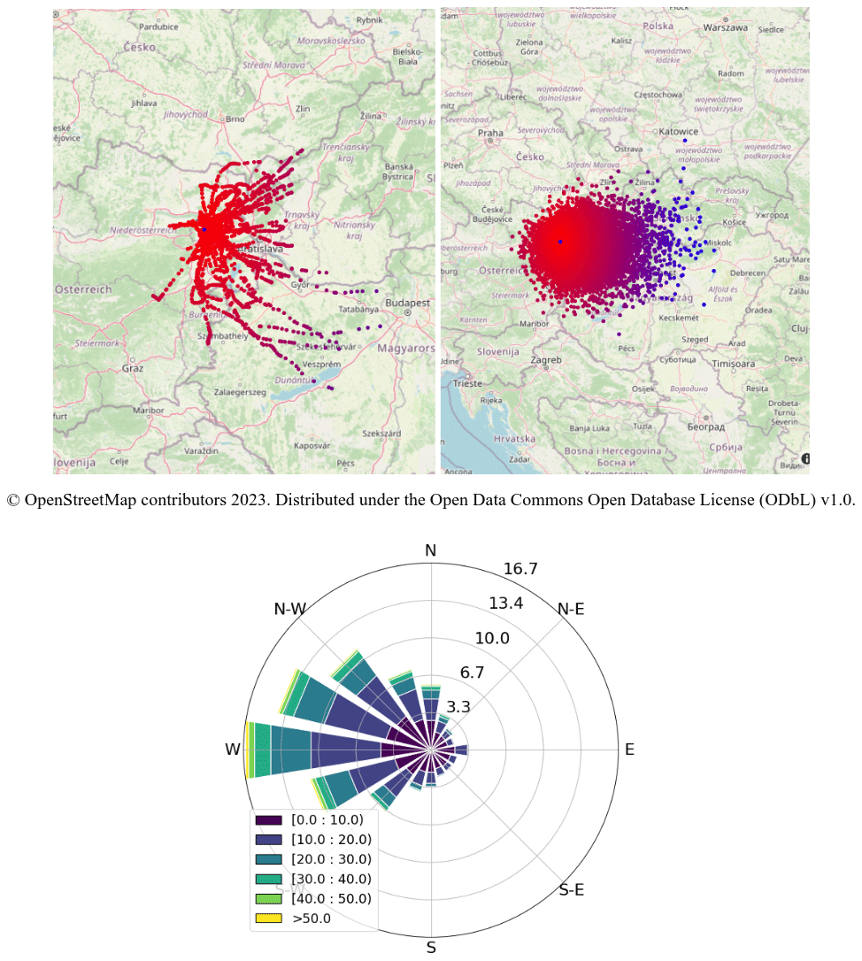
Figure 1 Upper panels: balloon displacements for station Vienna Hohe Warte, Austria (WIGOS ID 0-20001-0-11035). The central blue dot denotes the station's location, and the other dots are balloon positions calculated from wind data as explained in the text, coloured red to blue with increasing distance. Note that the area covered is non-isotropic around the launch site. Left panel: trajectories of all radiosonde ascents during the year 2000. Right panel: maximum displacements of all available ascents for all years between 1950 and 2021. Lower panel: wind rose of the Vienna Hohe Warte station for all available wind data. Colour indicates wind speed (m s⁻¹) and radius indicates the frequency distribution (%) of the direction, from where the wind (sectors) and wind speed (colours) come.

Radiosonde measurements are used in a variety of applications, including near real time by forecasters and numerical weather prediction (NWP), but also for air pollution or other scientific investigations, including climate monitoring (e.g. Dabberdt and Turtiainen, 2015). The production of climate reanalyses that directly assimilate radiosonde observations, such as ERA5 (Hersbach et al., 2020), is expected to benefit from more accurate historical balloon position data, similarly to NWP. In this regard, the location precision of the assimilated measurements should be commensurate with the horizontal resolution of next-generation reanalyses (∼ 10 to 20 km globally, e.g. Hersbach et al., 2022). At such resolutions, assuming vertical ascents for a balloon that is displaced by a couple of hundred kilometres would amount to comparing the balloon measurements with model values that are 10 or more grid boxes away, which is clearly suboptimal. Resolving this situation requires, for historical soundings, reconstruction of the balloon trajectories from the little information that is available (Stohl, 1998). In many cases, this information only consists of the vertical profile of wind, as discussed later in the paper.

Section 2 describes the data and a method to calculate the balloon drift from historical radiosonde ascent data. Details of the technical implementation, with Python code and test data, are provided in Sect. 3. Section 4 presents validation results, including several sensitivity analyses to explore the robustness and accuracy of the approach. Sections 5 and 6 show evaluation results, using two different approaches, whereby the beneficial impact of the more accurate balloon position is demonstrated. Section 7 includes a discussion and conclusions.

2 Data and methodology

2.1 Radiosonde data

Radiosonde data used in this work are obtained from the Integrated Global Radiosonde Archive (IGRA) Version 2 (Durre et al., 2016) and the Copernicus Climate Change Service (C3S) Climate Data Store (CDS). High-resolution radiosonde data used for validation are obtained in BUFR format from the National Centers for Environmental Information Radiosonde Archive (NOAA NCEI).

The quality of the available wind data depends on their encoding and the method used to track the balloons. Measuring techniques for upper-air winds have changed significantly over time, with a clear general trend towards improvements in quality thanks to removal of procedural errors in particular (e.g. Crutcher, 1979), noting also improvements in the accuracy of encoding, with evolution of the data formats. All these changes are described in the WMO Publication Nr. 8 Guide to Meteorological Instruments and Methods of Observation, published since 1954 by the WMO Commission for Instruments and Methods of Observation (CIMO; WMO, 2021). Regarding changes in the measurements of wind and balloon positions, there are three important distinctions to be made.

The first distinction concerns the sensing apparatus: non-GNSS versus GNSS sondes. Early observations used only ground-based tracking, e.g. by theodolite, which was fairly accurate but could lose the balloon early during cloudy or high-wind-speed conditions and relied on an assumed ascent rate if, like in most cases, a single theodolite was used (e.g. Favà et al., 2021). From the mid-1950s onward, radar tracking or radio positioning of the radiosonde became standard. Wind components were then calculated from the measured position and time differences.

In the 1990s, GNSS modules were introduced to track the horizontal and vertical positions of the sensor at high frequency, thanks to improvements and miniaturisation of the electronics. The resulting data were then used to calculate the wind variables, but the position data were not transmitted to the global network and are therefore not available in global databases in most cases until 2014.

The higher frequency of observations exchanged in recent years can expose the pendulum motion of the sonde beneath the balloon in its observed position (Ingleby et al., 2022). In our experimental cases, we did not observe any significant effect of the pendulum motion, its magnitude being generally much smaller than the wind advection displacements, suggesting it does not appear to need to be taken into account to first order.

The second aspect is the determination of altitude. Prior to GNSS observations, altitude was determined by three different methods: ascent speed estimation, pressure sensors, and vertical radar or radio positioning, with continued efforts to increase the quality of observations over time. Ascent speed can be affected by many factors, and Murillo et al. (2005) estimated a scatter in linear ascent rates of about 5 % about the mean value for pilot balloons after using double theodolites to conduct measurements to measure the balloon height during ascent.

The third aspect is the data format used for transmission. Essentially, two main message systems have been used to transmit the observed radiosonde data: Traditional Alphanumeric Code (TAC) and BUFR. The main difference is that BUFR allows not only for a much higher vertical resolution (up to 1 s frequency, corresponding to approximately 5 m altitude difference) but also for a higher coding precision. The BUFR messages report wind direction with a resolution of 1°, whereas TAC messages report wind direction to the nearest 5°. In addition, time and three-dimensional position information is only transmitted via BUFR but not via TAC. TAC messages typically also include data only on mandatory and significant levels. Mandatory levels are a set of predefined pressure levels. Significant levels for wind are added as needed before transmission so that the wind speed does not deviate by more than 5 m s⁻¹ from linearly interpolated values, according to the above-cited WMO CIMO guide.

There are also thermodynamically significant levels, which refer to specific levels of atmospheric pressure at which significant changes in temperature, humidity, or other thermodynamic properties occur. Most transmitted radiosonde profiles include some of these.

2.2 Quality control

The following steps are taken to exclude outliers.

• For wind speed, we applied a range check, with wind speed limited to 150 m s⁻¹, a value that is rarely reached, even in strong upper-level jets.

• For temperature, needed for geopotential calculations, we relied on the IGRA2 quality control (Durre et al. 2018) that already removes gross errors. A range check was also applied, with temperature limited to between 173 and 373 K, to verify that the data were read correctly and to avoid possible encoding errors in the messages.

Observations that fall outside these limits are not processed further to avoid degrading the quality of the output (balloon trajectory).

We investigated whether additional quality control measures would improve the performance and validation of the RMSE differences discussed in Sect. 5. To improve outlier removal, we filtered the observations based on the 1st and 99th percentiles of the difference observations minus ERA5 forecast (these differences are called background departures afterwards). This was completed in two stages: once for each level and then again for the entire set of available wind speed and temperature data. However, neither of the two versions improved the RMSE differences. Rather, we found that the background departures were often large enough to be discarded just in the interesting cases of strong but plausible displacements. The reason was not always the displacements themselves but also the fact that large lateral displacements can lead to large height errors in profiles from non-GNSS Russian radiosondes, since those have no pressure sensor but rely on radar heights (Kats et al., 2005). However, even for these sondes, we found that taking into account the balloon drift reduces the differences to the ERA5 background forecasts.

The results presented in Sect. 6 include the standard quality controls applied during data assimilation experiments, as detailed in the technical documentation published by ECMWF (2023).

Filtering radiosonde data before the displacement calculation based on the number of available observations per profile is recommended. A profile should not be too coarse and should not start too high above the ground. For the experiments conducted in this study, the limit for the initial observation was set at 1500 m above the release station height.

2.3 Estimation of the balloon trajectory

The balloon position is calculated relative to the launch position (so-called base coordinates) as latitude displacement and longitude displacement (decimal degrees). For each vertical level, these two values can be added to the base coordinates to obtain the new (latitude, longitude) position at the given level. The same approach applies to the reconstruction of the measurement times at all levels. This practice conforms to the BUFR encoding standard.

For the position calculation, the same simple physical laws that have been used to derive the reported wind components are applied. Only a few initial parameters are necessary for this.

• Station coordinates or the starting point of the sonde (latitude and longitude)

• Wind vector (zonal and meridional components denoted respectively as u and v), measured by the sonde at different pressure levels

• Measurement time (t) at different pressure levels

These variables enable calculation of how long the sonde was exposed to horizontal wind and therefore can be used to estimate the displacement of the sonde.

Older datasets especially often only contain the starting time of the ascent; time information is not available for any of the reported pressure levels.

To estimate the time elapsed since the release of the balloon, three variables are needed.

• The reported pressure levels (generally available from radiosondes) or heights (generally available from so-called PILOT balloons, also called PIBAL)

• The sonde ascent speed

• The surface pressure or station height (not strictly needed for displacement calculation since the first level is typically reported quite close to the surface)

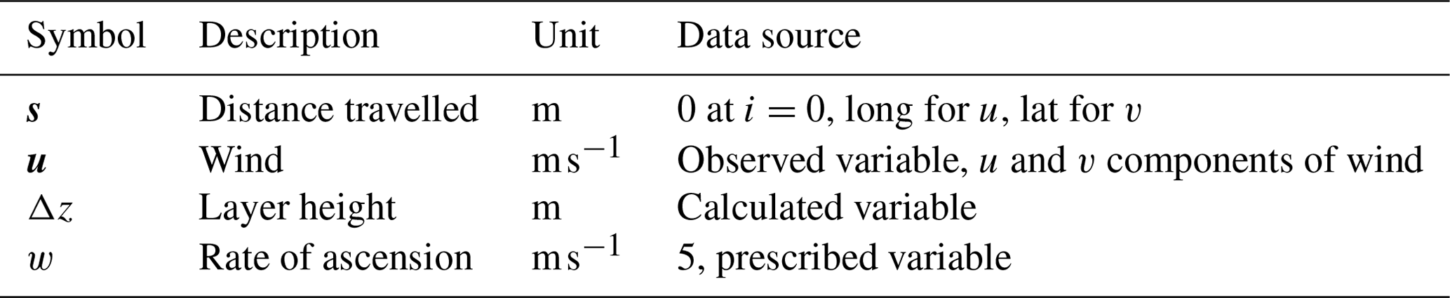
PILOT or PIBAL profiles provide an estimate of the height at each level, from which the time at each level can be reconstructed, assuming a given ascent speed. However, for multivariate soundings (radiosondes reporting temperature and wind), observed pressure is often the only information available regarding the radiosonde vertical position. In such a case, the pressure profile needs to be transformed to a height profile. This can be done by assuming a piecewise constant temperature gradient between the levels in the profile. The calculation of the vertical gradient of temperature with respect to altitude from the vertical gradient of temperature with respect to pressure is shown below in Eqs. (1) and (2). Subsequently, Eq. (3) indicates how this information is used to determine the heights of all the pressure levels. If the height information is already available (e.g. PILOT data), those steps can be skipped.

Table 1 Height profile calculation. Explanation of all used variables.

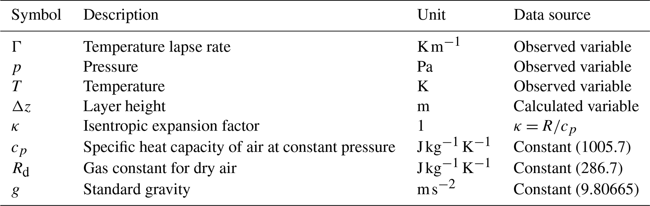
Equations (1) and (2) calculate the vertical gradient of temperature. See Table 1.

$$\begin{array}{}\text{(1)}& {\displaystyle }& {\displaystyle }{\mathrm{\Gamma }}_{\left(p\right)}={\displaystyle \frac{\mathit{\delta }T}{\mathit{\delta }z}}={\displaystyle \frac{\mathit{\delta }T}{\mathit{\delta }p}}{\displaystyle \frac{\mathit{\delta }p}{\mathit{\delta }z}}=-{\displaystyle \frac{\mathit{\delta }T}{\mathit{\delta }{p}^{\mathit{\kappa }}}}{\displaystyle \frac{\mathit{\delta }{p}^{\mathit{\kappa }}}{\mathit{\delta }p}}{\displaystyle \frac{\mathit{\delta }p}{\mathit{\delta }z}}\text{(2)}& {\displaystyle }& {\displaystyle }{\mathrm{\Gamma }}_{\left(p\right)}=-{\displaystyle \frac{\mathit{\delta }T}{\mathit{\delta }{p}^{\mathit{\kappa }}}}{\displaystyle \frac{p^{\mathit{\kappa }}}{T}}{\displaystyle \frac{\mathit{\kappa }g}{R_{\mathrm{d}}}}\end{array}$$

Equation (3) calculates the layer height. See Table 1.

$$\begin{array}{}\text{(3)}& \mathrm{\Delta }{z}_{(i\to i+\mathrm{1})}={\displaystyle \frac{T_i}{{\mathrm{\Gamma }}_i}}{\left({\displaystyle \frac{p_{i+\mathrm{1}}}{p_i}}\right)}^{-\frac{{\mathrm{\Gamma }}_i{R}_{\mathrm{d}}}{g}-\mathrm{1}}\end{array}$$

The vertical resolution of the available data varies. While early ascents often contain even less than the mandatory levels (16 levels), recent data in high-resolution BUFR are available on 3000 levels or more. The sensitivity of displacement calculations to vertical resolution is investigated later in this paper.

If a single mandatory level is missing within the ascent range, then the displacements are not calculated; we consider that too much information is missing in such a case. If a level was not mandatory in historical data (e.g. 70, 250, or 925 hPa), this rule does not apply to the data. However, an early termination of the vertical ascent is not an issue, and then the displacements are only calculated up to the highest available level.

The determination of the sonde's ascent speed is more uncertain. It depends on some variables that are poorly determined or unknown, such as the air vertical wind speed and the weight-to-buoyancy ratio of the probe and the balloon. Deviations in the filling level of the balloon, the air resistance of the balloon skin, as well as the ambient temperature and the balloon gas temperature further influence the ascent speed. A review of some of these factors was done by Favà et al. (2021).

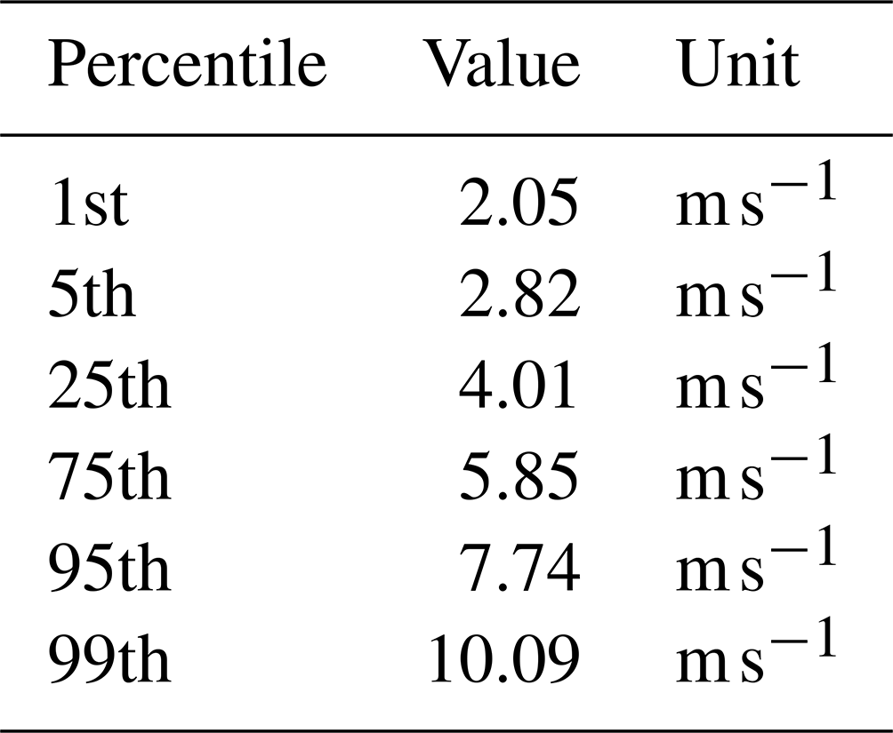
Using data from recent sondes, our study of the data with known altitude time series indicates that the rate of ascent varies mostly between 2 and 10 m s⁻¹. Within this large range, Fig. 2 shows that the mode of the distribution of ascent speeds is around 5 m s⁻¹. Table 2 further indicates that the interquartile range is 2 m s⁻¹ (i.e. from 4 to 6 m s⁻¹). These findings are consistent with other sources (e.g. Seidel et al., 2011). These statistics represent global fluctuations in the ascent speed of weather balloons.

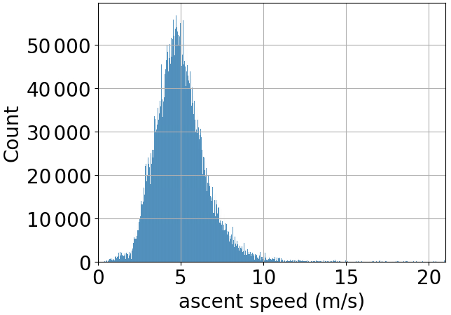
Figure 2 The observed ascent speeds from a sample of approximately 1010 000 000 BUFR-encoded observations with known altitude time series in 2020.

Table 2 Ascent speed percentiles for a sample of 10 000 000 observations with known altitude time series in 2020.

Over short timescales, Fig. 3 indicates that the vertical velocity of the probe fluctuates substantially. This is true both within a single ascent and also between different ascents. Near the ground and above the tropopause, the fluctuations are largest.

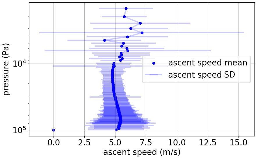
Figure 3 Mean ascent speed with standard deviation bars for all radiosonde ascents from Riverton, USA, in 2020, derived from high-resolution BUFR data.

Given the considerations above for historical balloons, one must recognize that the vertical speed can only be estimated in most cases and will always lead to significant deviations as compared with measurements obtained from high-resolution data. Note that the high vertical resolution shown in Fig. 3 is hardly reached in ascents before the year 2000. This also means that, if only mandatory levels are available, the fluctuations in the average ascent speed at each available level are smaller due to the longer averaging intervals.

Figures 2 and 3 show that an assumed ascent rate of 5 m s⁻¹ agrees well with the observed mean value. To counteract the effects of this fluctuating parameter, an attempt was made to use a height-dependent function instead of a constant speed, which represents the annual average over more than 100 stations.

As part of this experiment, a polynomial model was also tried in an attempt to improve the accuracy of the average ascent speed. The resulting displacements showed, however, very little improvement (i.e. smaller differences to GNSS-measured displacements), indicating that the assumed vertically constant ascent rate of 5 m s⁻¹ is a sufficient approximation.

As a next step, it is necessary to calculate the height profile from temperature and pressure information. For this step, we use the equation for a dry atmosphere with a piecewise constant lapse rate (Alexander and de la Torre, 2011). Relative humidity could also be considered by using the virtual temperature, but it is often not available for early ascents, and we also found that the differences in the resulting displacements were small. For the first level, the International Civil Aviation Organization (ICAO; Tahler, 2019) standard atmosphere lapse rate of −0.0065 K m⁻¹ is used. For all subsequent steps, the temperature gradient is calculated directly from the temperature and pressure profile (mean values for each layer “i”).

The height profile is then used to calculate the time interval spent by the sonde between the noted levels. It can be estimated using the estimated vertical velocity mentioned earlier.

These time intervals are then used to determine the transport of the balloon according to the mean wind inside the layer between the levels i and i+1: see Eq. (4).

Table 3 Time interval calculations and explanations of all the used variables.

Equation (4) shows the transport of the balloon with the wind. See Table 3.

$$\begin{array}{}\text{(4)}& {\mathit{s}}_{(i+\mathrm{1})}={\mathit{u}}_{(i\to i+\mathrm{1})}\cdot {\displaystyle \frac{\mathrm{\Delta }{z}_{(i\to i+\mathrm{1})}}{w_{\text{balloon}}}}\end{array}$$

Afterwards, this distance is converted into latitude and longitude using either the inverse Haversine method on an assumed sphere or the forward transport function on the WGS84 ellipsoid. The difference between the two transport functions is found to be practically invisible for smaller observed displacements (see Fig. 4). Nevertheless, the ellipsoid option is used as it should deliver higher-accuracy results. Finally, the resulting latitudes and longitudes are subtracted from the base coordinates to obtain the displacements.

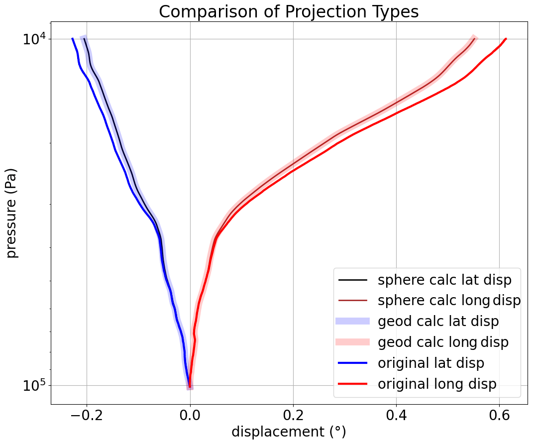
Figure 4 Calculated displacements (black and brown for spherical earth, thick light blue and red for WGS84). Observed displacements stored in BUFR displacements (blue and red) are included for comparison. Tallahassee, Florida, USA, 31 May 2020, 23:19:00 UTC.

Particular care is required when using reported wind directions near the North Pole or South Pole. For example, when crossing the North Pole, a radiosonde in a southerly airflow (prior to the crossing) finds itself in a northerly airflow (afterwards). So far, only TAC has been used at the South Pole station, which means that the wind components are reported according to the launch position, not the actual position, and are thus constant during the ascent. We calculate the displacements in the x and y directions valid at this position and then convert them back to latitude–longitude positions and displacements.

The WMO Manual on Codes states that, for stations within 1° of either pole, wind direction shall be reported in such a way that the azimuth ring shall be aligned with its zero coinciding with the Greenwich 0° meridian. There is currently an attempt to update this advice for BUFR reports, such that wind direction should be reported relative to the current reported longitude – to help in NWP use of such winds. Before comparing winds from the South Pole station with NWP fields, they should have their direction adjusted when the drift positions are calculated, but note that this was not done in the present work.

Although the principle of displacement calculation is similar to the method presented in earlier work on this topic (Laroche and Sarrazin, 2013), we use different input data for height information. Instead of using the average ascent time for each standard level, we calculate the times for each available level using the mean lapse rate for the representative layer.

Aberson et al. (2017) applied a similar approach for dropsondes, albeit with a different way of calculating the vertical velocity.

Both of these methods are successful and promising, and for the purpose of this method they have been used as the basis for reconstructing the trajectories as well as possible.

3 Implementation and availability

The software necessary for the creation of calculated balloon trajectories can be found in the Python package rs-drift.

• https://doi.org/10.5281/zenodo.10663306 (Voggenberger, 2024)

• https://pypi.org/project/rs-drift/ (last access: 6 May 2024)

Examples of how to use it are available in all the repositories as the IPython notebook rs_drift_example.ipynb.

In addition to the coordinates of the launch site or station in degrees latitude and longitude, the trajectory function requires profiles of four input variables in the right units: temperature (K), pressure (Pa), zonal wind (u; m s⁻¹), and meridional wind (v; m s⁻¹). It accepts only input which is sorted in ascending order.

$$\begin{array}{rl}\text{trajectory }=& \text{ rs\_drift.drift.trajectory(lat,lon,temperature,}\\ & \text{ u,v,pressure)}\end{array}$$

The function returns the following output.

$$\begin{array}{rl}\text{trajectory }==& \text{[latitude\_displacement, }\\ & \text{longitude\_displacement, seconds\_since\_start]}\end{array}$$

All those output variables are numpy arrays, with one element for each pressure level – with the same length as the input data. For PIBAL ascents, the geopotential height must be provided as an additional keyword parameter.

It is possible to experiment with input data. If humidity information is available, the virtual temperature can be used instead of the observed air temperature. Also, if more information on the balloon's mean ascent rate is present, this should be used as input in the additional arguments. Any approach including proper quality control of input data that are available should be used to create the best possible estimation of the balloon drift.

The drift of the balloon and sonde compounds is introduced as a “displacement” from the starting point (launch site). For simplicity, the displacements can be added to the base coordinates to obtain the vertical profiles of positions of the balloon.

4 Validation with GNSS radiosondes

Validation per se is only possible when a trusted source can provide a good reference. Such is the case for modern sondes equipped with GNSS receivers when it comes to the recovery of balloon trajectories. For pre-GNSS radiosondes, a similar validation would be possible only if one had available the information about the balloon trajectory. Unfortunately, this information is only available in rare cases.

The data from the modern GNSS radiosonde data encoded in the recent high-resolution BUFR files are used to verify the systematic and random errors of the calculated displacements at different pressure levels. This dataset contains second-by-second records of actual positions of the sonde measured by the GNSS in the form of displacements, thus enabling the direct comparison with the calculated displacements.

Figure 4 also shows that the displacements obtained from the GNSS and the displacements calculated from the wind data agree quite well. The small deviations likely come from differences between the actual (unknown) and assumed (5 m s⁻¹) ascent rates.

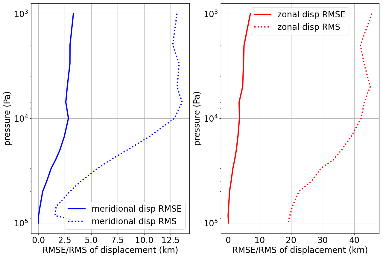
Figure 5 The rms of meridional (blue dotted) and zonal (red dotted) displacements and the RMSE between observed (from GPS) and modelled displacements (solid blue and solid red respectively). The samples contain all BUFR-encoded ascents in the summer months of 2020 (more than 10 000).

Figure 5 provides an overview of how large the displacements typically are and shows profiles of uncertainty estimates for the calculated displacements. In the troposphere the RMSE is mostly below 0.02° (2.5 km), and in the stratosphere it can be up to 0.1° (12 km). These numbers amount to uncertainties of about 1 part in 5 to 10, of the observed variations (rms), in the example shown. Still, this is much better than just ignoring the displacement.

These results were obtained by using as input the high-resolution data. For historical radiosondes, only comparatively low-resolution information is available (in the form of mandatory plus significant levels).

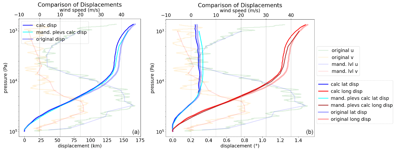
Figure 6 Vertical profiles of displacements (starting at zero at the surface), calculated from observed winds (thin lines) or taken from BUFR thick light lines. The profiles of observed wind (thin light colours) are plotted to the upper x axis – Peachtree City, Georgia, USA, on 31 January 2021, 23:24:00 UTC. (a) Overall displacements (km). (b) Latitude and longitude displacements (°) as encoded in BUFR.

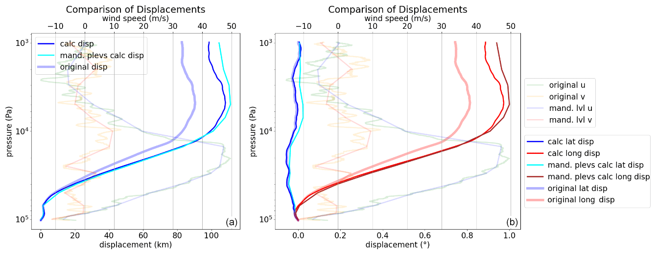
Figure 7 Vertical profiles of displacements (starting at zero at the surface), calculated from observed winds (thin lines) or taken from BUFR thick light lines. The profiles of observed wind (thin light colours) are plotted on the upper x axis – Ishigaki, Okinawa, Japan, on 31 December 2019, 23:31:00 UTC. (a) Overall displacements (km). (b) Latitude and longitude displacements (°) as encoded in BUFR.

In Figs. 6 and 7, the impact of using only mandatory and significant level information is shown. The difference of displacements in Fig. 6 is minimal, although the displacement is relatively large.

Figure 7 shows a case of larger differences in relative terms. The overall zonal displacements are large and the winds vary strongly with altitude. An issue arises when selecting data points with low representativeness from the ascent, particularly those that are far from the layer average. This can result in less accurate outcomes compared with using averages from less detailed data. Figure 7 provides a good example of this issue with the v component of wind at the original resolution and mandatory pressure levels only. The method for calculating the displacements themselves uses mean wind speeds on the considered levels. Thus, if the observations are also means of larger vertical height differences, more or less randomly observed peaks become a smaller source of error.

Figures 6 and 7 respectively show the range of accuracy of the calculated trajectories quite well. The final displacements may differ in quality, depending on the quality of the observations, the representativeness of the available levels, and the vertical resolution. All ascents in the validation examples had displacements, which added value in bringing the observation closer to the true position. The accuracy may vary based on the aforementioned input variables. However, we did not find any cases where using the displacements would lead to a worse position estimate.

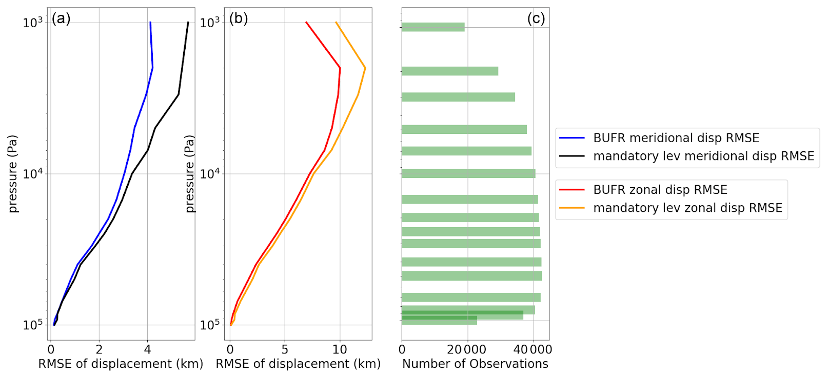
Figure 8 RMSE between observed and modelled displacements of meridional (a) and zonal (c) components, averaged over all stations available in October 2014, one of the first months with a sizable number of high-resolution BUFR-encoded profiles. Blue and red are RMSE profiles obtained by using the full vertical resolution of BUFR observations, and black and orange are RMSE profiles and obtained by using only mandatory level information.

Figure 8 shows the comparison between the displacements of two different datasets – on the one hand on high-resolution BUFR levels and on the other hand on mandatory levels only. It can be seen that for this subset of ascents there is still much value in the displacements for the mandatory-level-only version. However, it should be noted that more available levels always lead to better results and that the highest possible number should be used in any case.

Many of the older observational reports contain temperature and wind data on different levels. Only at mandatory levels are both variables available. In this case, interpolation can be performed for the points in between. When applied to IGRA data, wind data are interpolated to the levels of the temperature observations. This allows the input to be maximised to calculate the best possible displacements.

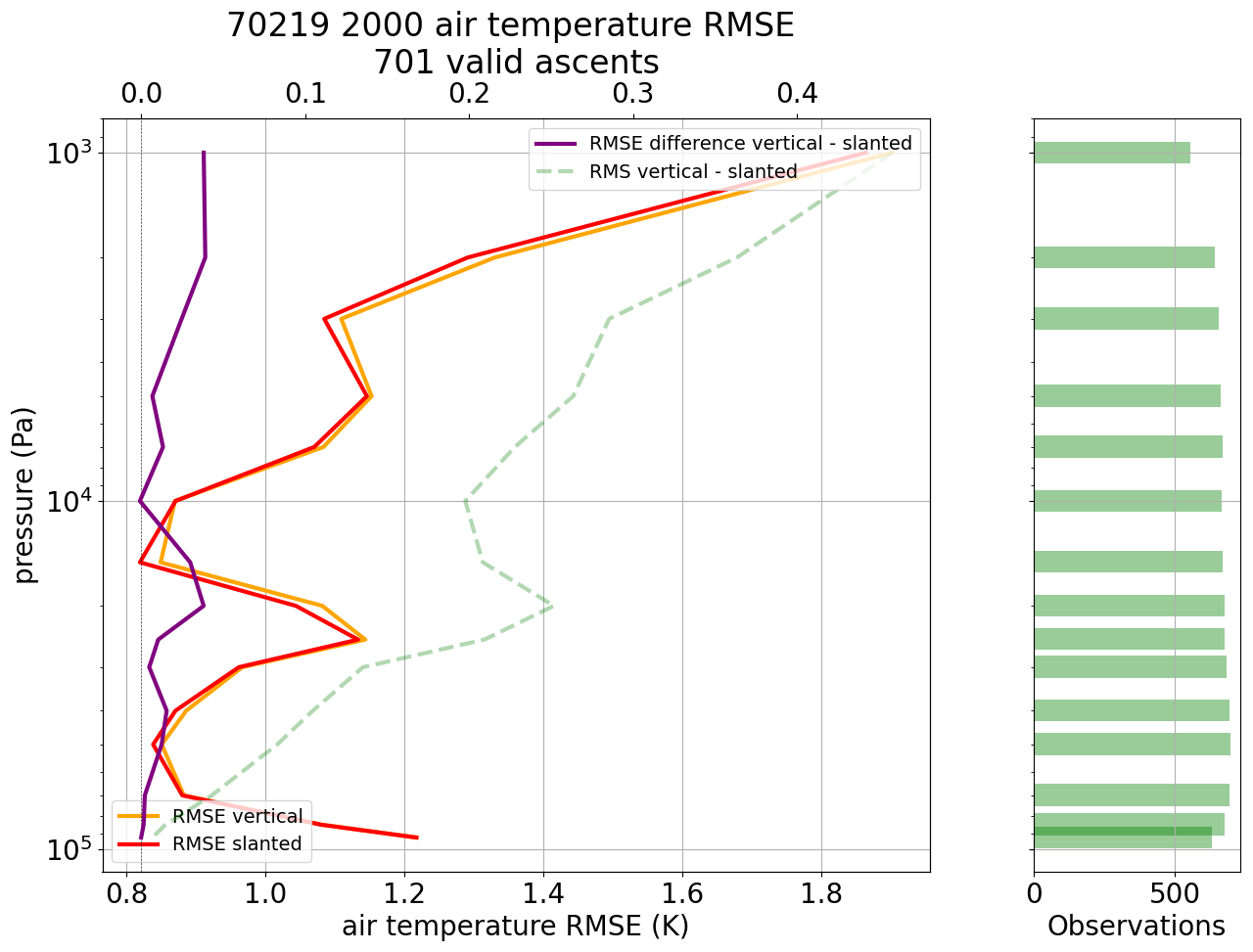
Figure 9 Bethel Airport, Alaska: all 2020 ascents. RMSE (obs − ERA5) of base coordinate temperatures minus sonde temperatures (orange) and RMSE (obs − ERA5) of displaced temperatures minus sonde temperatures (red) as well as the rms of displaced minus base (green dashed line) to show the magnitude of the difference between base and displaced temperatures. A positive difference between the orange and red graphs (purple line, upper x axis) shows improvement due to more accurate balloon positions. The green bars on the right indicate sample sizes at different levels.

5 Evaluation with ERA5

To evaluate the impact of taking the displacements into account, we compared the observed values from the radiosondes with the gridded ERA5 data, in one case assuming a strictly vertical ascent and in the other case assuming an ascent along the calculated (slanted) trajectory defined by the displacements. The ERA5 fields at hourly resolution and 1° × 1° horizontal resolution were interpolated linearly horizontally to the observations locations defined in either of the two cases mentioned earlier (vertical or slanted).

These tests and comparisons used the short-term forecast of the ERA5 assimilating model, also referred to as the “background”. This choice, instead of using ERA5 analyses, was made to try to maintain as much independence as possible with respect to the observations. This choice should largely avoid possible problems resulting from the fact that the observations are also assimilated into the ERA5 data, given that many other observations were assimilated alongside radiosondes and also influenced the analysis state. Experimental comparisons with the ERA5 analyses (in contrast to the background forecasts) showed that the analysis data fit significantly better with the vertical trajectory of the observations than with the slanted version. This is to be expected, since radiosondes were assimilated as vertical profiles in ERA5.

Figure 9 shows the benefit of comparing the radiosonde observations with the background forecasts as slanted profiles instead of vertical profiles. In low layers (below 700 hPa), the displacements are relatively smaller than at higher levels and therefore hardly lead to deviations for temperature. In most cases, there is an improvement at levels located above 750 hPa, though at some stations the improvement is already visible as soon as the sonde reaches 850 hPa, depending on the wind speed and topography around the station. Typically, the effect is largest in regions with high upper-level wind speeds. Taking the displacements into account improves the background departure statistics between the measurements and ERA5, not only for temperature, but also for wind and relative humidity.

For relative humidity, the improvement is confined to levels located below 250 hPa. Above this level, the relative humidity is generally very low, making it difficult to detect any meaningful difference with respect to the ERA5 background.

It is also important to note that some stations, where the RMSEs of the ascents do not show signs of improvement in temperature, often still show improvement in humidity or wind (or vice versa).

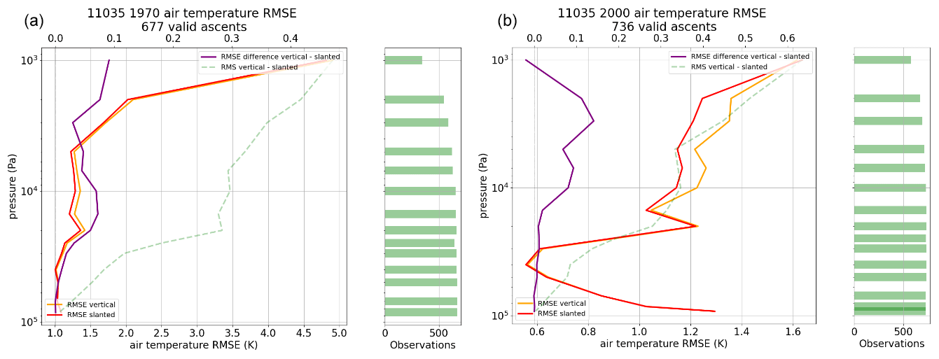
Figure 10 Vienna Hohe Warte, Austria – (a) all 1970 ascents; (b) all 2020 ascents. Different x-axis scales are used. RMSE (obs − ERA5) of temperature assuming vertical ascents (orange, lower x axis) and RMSE (obs − ERA5) of temperature from slanted ascents, taking balloon drift into account (red, lower x axis). A positive difference between the orange and red graphs (purple line, upper x axis) shows improvement due to a more accurate balloon position.

Considering that radiosonde observations make up the larger part of the total number of observations for the reanalysis in earlier years, one might think that, especially for these years, the displacements are more relevant. The data investigation reveals that improvements in the departure statistics are not greater for earlier ascents than for more recent ascents. The reason might be that reanalysis fields before the satellite era are more strongly dependent on radiosondes. At these times few other upper-air observations were available, and radiosonde data were assimilated assuming vertically straight ascents. However, the density of the input data and the general quality of the reanalysis increased over time, while the bias in measurements of the uppermost levels decreased over time. Therefore, the relative importance of representation uncertainties, with respect to the two other sources of uncertainties in the comparison (radiosonde instrumental uncertainties and ERA5 background uncertainties), is greater for more recent ascents. Figure 10 shows that considering the displacements is also beneficial, although to a lesser extent, in the early days, when little upper-air information other than from radiosondes was available.

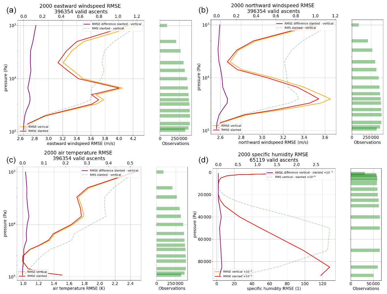
Figure 11 Finally, in Fig. 11 there are the results of a global comparison for the year 2000 – like the previous ones but calculated for all the available stations. A positive difference again indicates improvement due to taking the displacements into account.

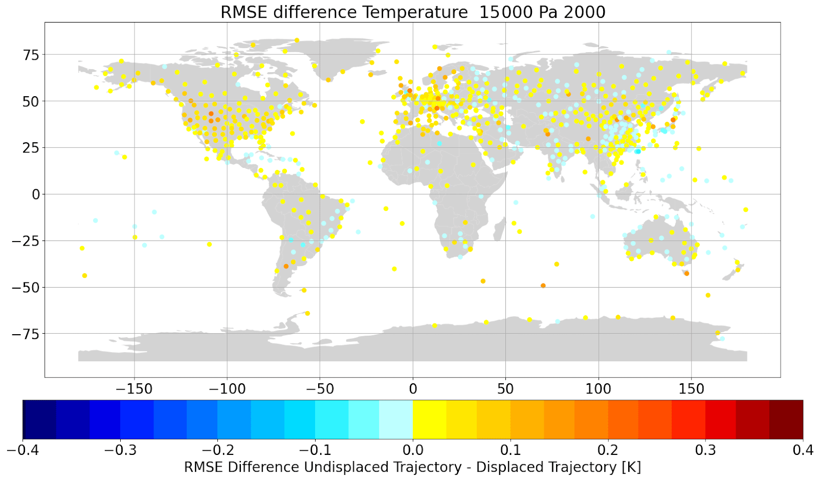
Figure 12 Global station difference of temperature (K) observation RMSE (obs − ERA5) when compared with the background at station coordinates minus the temperature observation RMSE (obs − ERA5) when compared with the background at a displaced position. Positive values indicate improvement due to a more accurate balloon position. All available observations at 150 hPa averaged over all ascents in the year 2000.

Finally, in Fig. 11 there are the results of a global comparison for the year 2000 – like the previous ones but calculated for all the available stations. A positive difference again indicates improvement due to taking the displacements into account.

To give a better insight, the differences of the RMSE are also plotted on a map for the 150 hPa level in Fig. 12. Warm colours show improvement for the respective station by applying the displacements, and cold colours show a deterioration. Improvement clearly predominates for the majority of the stations. Deteriorations in quality appear less frequent and of smaller magnitudes than improvements.

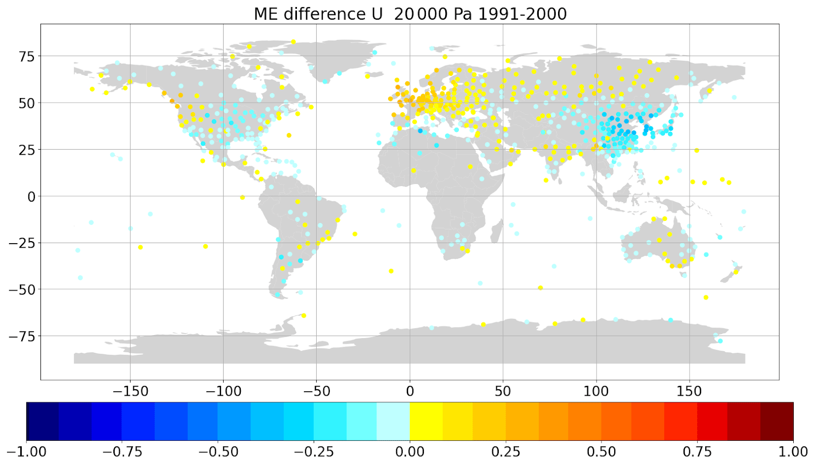
Figure 13 Mean zonal (u) wind (m s⁻¹) difference obs − ERA5 background at the station position minus the obs − ERA5 background at a displaced position. All available values at 200 hPa of years 1991–2000.

Figure 13 shows the difference of the ERA5 background eastward wind speed in the 1990s at the station location minus the same wind speed at the displaced location. The differences are sizable in some regions. For example, the weaker wind speeds above the station locations in China would indicate systematically too high observed wind speeds. This effect is large enough to explain some of the radiosonde wind–background wind differences, as pointed out by Tenenbaum et al. (2022). This stresses again the importance of avoiding position errors in historical radiosonde ascents. Without the adjustments, artificial trends in wind speed from radiosondes would be introduced in some regions when switching from traditional to GNSS radiosondes.

6 Evaluation with data assimilation experiments

Desroziers et al. (2005) proposed a method to diagnose uncertainty statistics of observations in a data assimilation framework. As indicated in their work, there are important assumptions associated with the approach. Bias contributions aside, the overall level of uncertainty may be incorrect if, for example, there is a significant correlation between observation random uncertainties and random uncertainties of the background that is used in the data assimilation. A separation of scales is indeed required in order to disentangle these two uncertainty components. Given the unique importance of radiosondes for informing the state of the stratosphere in a background obtained from data assimilation, such as in a reanalysis (e.g. Hersbach et al., 2020), there may be some components of the uncertainties (such as radiation) that are present, and possibly correlated, in the background and the observations. For these reasons, we do not use Desroziers' diagnostics in order to assign indisputable uncertainties to the radiosonde uncertainties. Instead, we use these diagnostics in order to detect any changes in the observation uncertainties, which include instrument and representativity uncertainties, owing to the effect of balloon drift.

To this end, we run two data assimilation experiments using a simplified data assimilation setup. Simplifications are required in order to make such an undertaking numerically affordable. Otherwise, so-called “full” data assimilation experiments, using all observations at the maximum resolution, are indeed too costly to conduct, if only for such an evaluation. The simplified data assimilation setup is based on the ECMWF Integrated Forecasting System (IFS) cycle 48R1 configuration (ECMWF, 2023) using an octahedral reduced Gaussian grid with 159 wavenumbers, or a horizontal resolution of approximately 69 km, instead of the ECMWF operational configuration which has a resolution of approximately 9 km at present. Also, similarly for affordability reasons, the experiments only assimilate conventional observations (no satellite observations), the number of four-dimensional variational (4D-Var) minimisations is reduced from three to two, and the analysis increments are at a resolution of approximately 210 km (instead of 39 km for ECMWF operations). The simplified data assimilation setup enables us to run data assimilation experiments for a duration of 2 months, 1 June–31 July 1980.

The first experiment is the control. It assimilates the radiosonde observations as vertical profiles. The second experiment assimilates the radiosonde observations following the balloon trajectory when this information is available (otherwise the data are assimilated as vertical profiles). The balloon drift in the assimilation is handled by dividing the whole ascent into 15 min sub-profiles (Ingleby et al., 2018). In each sub-profile, the latitudes, longitudes, and times are invariant. In spite of this arrangement, which only partially reflects the true slanted nature of the profiles, we retain the terminology of “slanted profiles” when discussing the results, for clarity within this paper.

Table 4 Statistics for the radiosonde observations actively used by both data assimilation experiments (vertical and slanted), distinguishing between radiosondes launched from land stations and radiosondes launched from ships. P indicates the pressure (hPa), RSD indicates the robust standard deviation of background departures (i.e. before assimilation), SIGO indicates the estimated observation uncertainty (see the text for details), and N indicates the data count. Results that differ between the two experiments are shown in bold. Observations that were used by only one of the two experiments are excluded from these statistics.

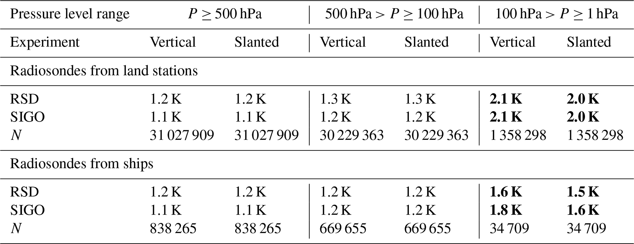
Here we consider the radiosonde observations that were assimilated in both experiments to ensure that no difference in the results may be caused by sampling differences. Table 4 shows the statistics for these data. For the reasons mentioned earlier, the interpretation of the table focuses on differences between the two experiments and not on the absolute level of observation uncertainties determined by Desroziers' diagnostics. At 0.1 K, we find no detectable difference between the two experiments for the levels located below the 100 hPa pressure level. For levels located higher, i.e. at pressures lower than 100 hPa, we find that background departures and estimated observation uncertainties are reduced in the experiment that assimilated the data along slanted profiles. This result is obtained for radiosondes launched from land stations as well as radiosondes launched from ships.

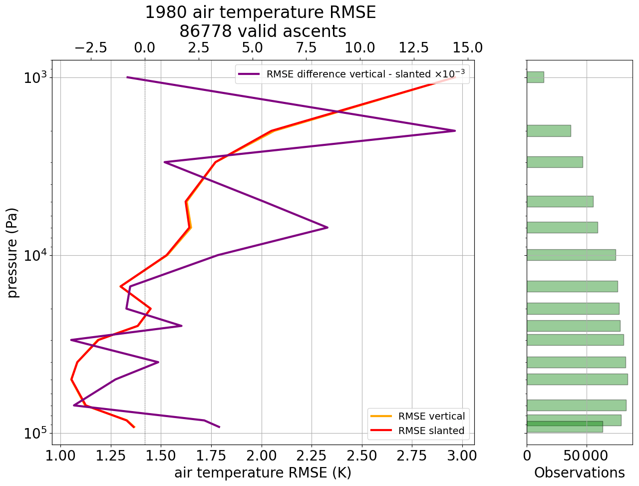
Figure 14 Air temperature obs − bg RMSE difference for experiment “vertical” (orange) and for experiment “slanted” (red). The difference of differences (orange − red) yields the purple line on the upper x axis: note the scaling factor 10⁻³. Positive values indicate improvement due to a more accurate balloon position. All available stations are at mandatory pressure levels between 1 June 1980 and 31 July 1980.

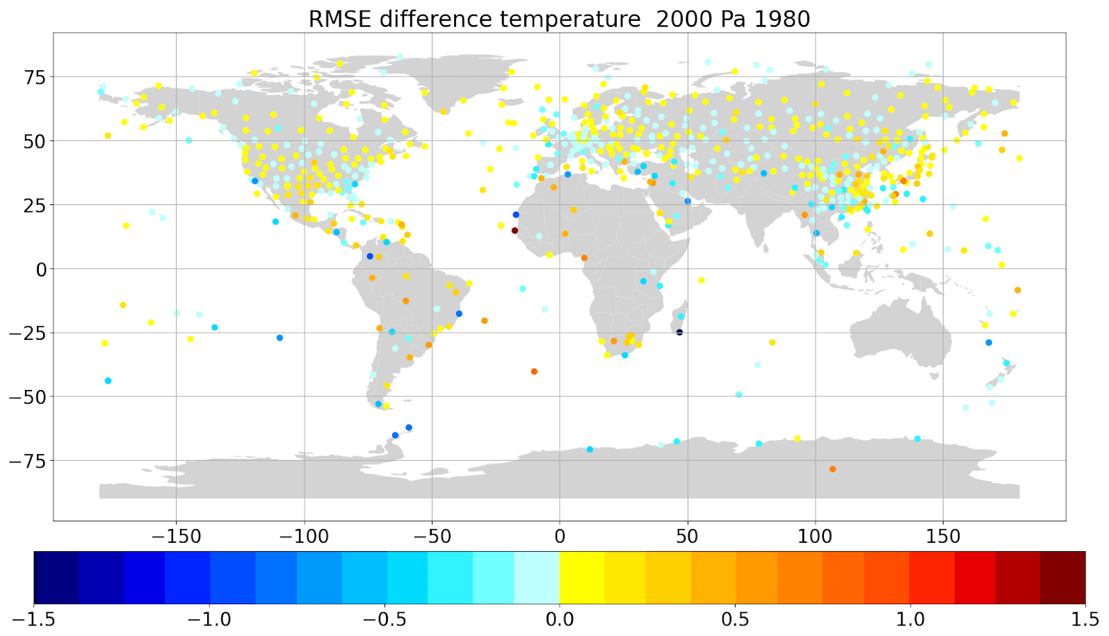
Figure 15 Air temperature obs − bg RMSE (K) difference of experiment “vertical” minus the RMSE of experiment “slanted”. Positive values indicate improvement due to usage of a more accurate balloon position. All available stations at 20 hPa between 1 June 1980 and 31 July 1980.

The differences may appear to be very small and could be discarded as unimportant if it was not for the fact that reducing observation and representation uncertainties is generally an impossible task once observations have been collected and already processed once. The present findings demonstrate that it is possible to generate a greater return in terms of information content through reprocessing of the observations. The reprocessing here enables us to assimilate observations along a slanted trajectory. Furthermore, these are global statistics – see Fig. 14. The previous sections indicated that the results may vary by launch site. Consequently, the improvements shown here, for global statistics, must hide some greater improvements at some particular sites – see Fig. 15.

Given previous results indicating a larger effect of the balloon drift during winter seasons (e.g. McGrath et al., 2006) and given the much greater number of radiosonde stations in the Northern Hemisphere as compared with the Southern Hemisphere (e.g. Fig. 12), the present choice of the data assimilation season (Northern Hemisphere summer, as in Choi et al., 2015) represents a conservative approach. An impact of larger magnitude may be expected at different time periods, in particular during Northern Hemisphere winter.

7 Discussion and conclusions

The verification and evaluation results have shown quite clearly that, if at all possible, balloon displacements should be taken into account for all relevant data assimilation applications to minimize representation errors. Ignoring the possibility of accounting for observation location errors on the 100 km scale would be anachronistic, when global or regional reanalysis datasets approach spatial resolutions finer than 20 km.

The method to reconstruct the balloon position presented in this work is limited by a few assumptions and depends on the vertical resolution of the available profiles and the conformance of the weather balloons to modern ascent speeds. For the applications tested, an attempt was made to obtain the best results globally, and a clear positive impact was found, particularly when compared with ERA5 in the early 2000s, although positive results were also found at other times (e.g. the 1980s). This is also consistent with other findings in similar settings where trajectory data are used to reduce representation errors (e.g. Laroche and Sarrazin, 2013).

The data assimilation experimental setup employed here is a simplified one as compared with what may be used in a present-day reanalysis configuration such as ERA5. However, we observe a positive impact of the balloon drift in terms of reducing the background departures and the observation uncertainty, using Desroziers' diagnostics, for temperatures in the stratosphere. We expect that the quality of the corrections made to use radiosondes at a displaced horizontal position, as compared with using them at a vertical position, will increase when the background resolution and/or the background quality are increased. In addition, assessing the impact of the balloon drift sensitivity to the assimilation of other observations alongside radiosondes would be worth analysing. However, owing to time and computational constraints, it was not possible to investigate further these effects with full data assimilation experiments at higher horizontal resolution and using all available information, but we note that this would be a useful pursuit.

The results of the tests have shown that the method is successful in reconstructing displacements and improving the accuracy of the atmospheric data. Whilst the additional information provided by the method may not always be a visible improvement for individual comparisons, it is of significant value when the displacement changes the grid box of the model being compared. This has been demonstrated by improved means in the plots and better agreement between observations and ERA5.

The value of improving radiosonde observations by reprocessing of the positions was evaluated by conducting reduced-resolution data assimilation experiments covering a 2-month period in summer 1980. In the future, it would be desirable that the impact of similar activities that seek to improve the observational record be more regularly evaluated in the generation of downstream climate products. Such an evaluation should consider a longer time period and include the impact on low-frequency variability in the products. For products such as reanalyses, obtained via data assimilation, this should entail full-resolution observing system experiments (OSEs). For other types of climate products, including those powered by new opportunities such as artificial intelligence or machine learning (e.g. Singh et al., 2022), it is important that mechanisms be found to evaluate the impact of using the observations and how changes made in their handling affect the outcome.

Further experimentation using observation data from the period 2000–2020 is crucial and is likely to produce more compelling outcomes. The effective use of this method for informing future climate reanalysis is one of the main objectives.

As the world faces increasing challenges related to climate change, the importance of accurate atmospheric data and the potential of new methods to improve them cannot be overstated. The use of improved position metadata with radiosonde observations can account for previously unexplainable phenomena, demonstrating the potential of this method to shed new light on atmospheric data analysis. In addition, the method has the potential to improve the accuracy of reanalyses and climate predictions, which are crucial for many socio-economic sectors.

To achieve the optimal representation of the data, precise details regarding time and location must be available for every observation. One significant issue concerns the TAC format's transmission and storage of data, which often only include a nominal timestamp such as 00:00 UTC or 12:00 UTC. However, the actual launch of the respective balloon in most of the cases took place 30–60 min earlier. The precise time difference from the nominal time is frequently unknown, and therefore the displacement information cannot be utilised to its fullest extent. Since temperature can vary by more than 1 K h⁻¹ in the boundary layer just due to the diurnal cycle, this issue should be addressed. There are well-known examples where changes in the sampling of the diurnal cycle introduced spurious trends into climate data products (Mears and Wentz, 2005). Whenever possible, the precise launch time should be used. In cases where this information is not available for individual ascents, the time difference between the nominal and actual launches can often be determined from earlier or later ascents. Operators are normally advised to minimise the variation throughout the launch procedure and, therefore, launch balloon sondes at the same time every day.

Additional work to better understand the causes of variation in balloon ascent speeds (e.g. Zhang et al., 2019) could help further improve the results. Also, given all the uncertainty sources, it could be possible to generate an ensemble of trajectories for each ascent. Pendulum motion is an effect that would need to be better understood, as it could be of importance, e.g. in geographical locations where wind advection leads to small horizontal displacements.

The same approach as presented in this paper can be used to reprocess rocketsondes, dropsondes, ozonesondes, or any other in situ sonde advected by the wind, provided the necessary information is available. Taking into account the accurate balloon position would also be beneficial when comparing radiosonde observations with GNSS radio occultation (RO) observations (Gilpin et al., 2018). Indeed, while it is established practice to consider the tangent point drift of the RO data (e.g. Poli and Joiner, 2004), radiosonde data are frequently presumed to move vertically only.

In conclusion, the development and testing of the method for reconstructing displacements based on the wind profile shows promising results. The results presented in this paper suggest taking balloon displacements into account when producing meteorological or climatological data based on upper-air in situ balloon-borne observations.