What is the relative impact of nudging and online coupling on meteorological variables, pollutant concentrations and aerosol optical properties?

Meteorological and chemical modelling at the regional scale often involve the nudging of the modelled meteorology towards reanalysis fields and meteo-chemical coupling to properly consider the interactions between aerosols, clouds and radiation. Both types of processes can change the meteorology, but not for the same reasons and not necessarily in the same way. To assess the possible interactions between nudging and online coupling, several simulations are carried out with the WRF–CHIMERE (Weather Research and Forecasting) model in its offline and online configurations. Through comparison with measurements, we show that the use of nudging significantly improves the model performances. We also show that coupling changes the results much less than nudging. Finally, we show that when nudging is used, it limits the variability in the results due to coupling.

1 Introduction

The regional modelling of atmospheric pollution includes the modelling of meteorology and chemistry transport. If the chemistry-transport model (CTM) receives information from the meteorological model but does not send it back, it is an offline model. If, on the other hand, the two models exchange information, we are in an online modelling mode. Being regional, the models need forcing at the boundaries of the domain (the lateral and top boundaries) and inside the domain. For the meteorological part and inside the domain, the technique used is called nudging, and it can be “grid” or “spectral” (von Storch and Zwiers, 2001; Kruse et al., 2022). With spectral nudging, the meteorology can evolve due to mesoscale turbulence, but large-scale atmospheric circulations remain consistent with the global modelling that serves as forcing. Given that the global model has been corrected by data assimilation, the meteorological fields already implicitly contain the effects of aerosols on meteorology (Fig. 1).

On the other hand, for chemistry-transport modelling in online mode (which is increasingly used today and corresponds to the direct and indirect effects of aerosols on the meteorology), aerosols will modify the meteorology within the simulation domain. These changes are performed at higher spatial and temporal scales than the global forcing, which is intrinsically a large-scale process. Above all, they are completely independent of the large-scale circulation. It is therefore possible to have a contradiction between the scales: aerosols will modify the meteorology on the small scale, while, at the same time, nudging will constrain the large scale to remain close to the initial global forcing.

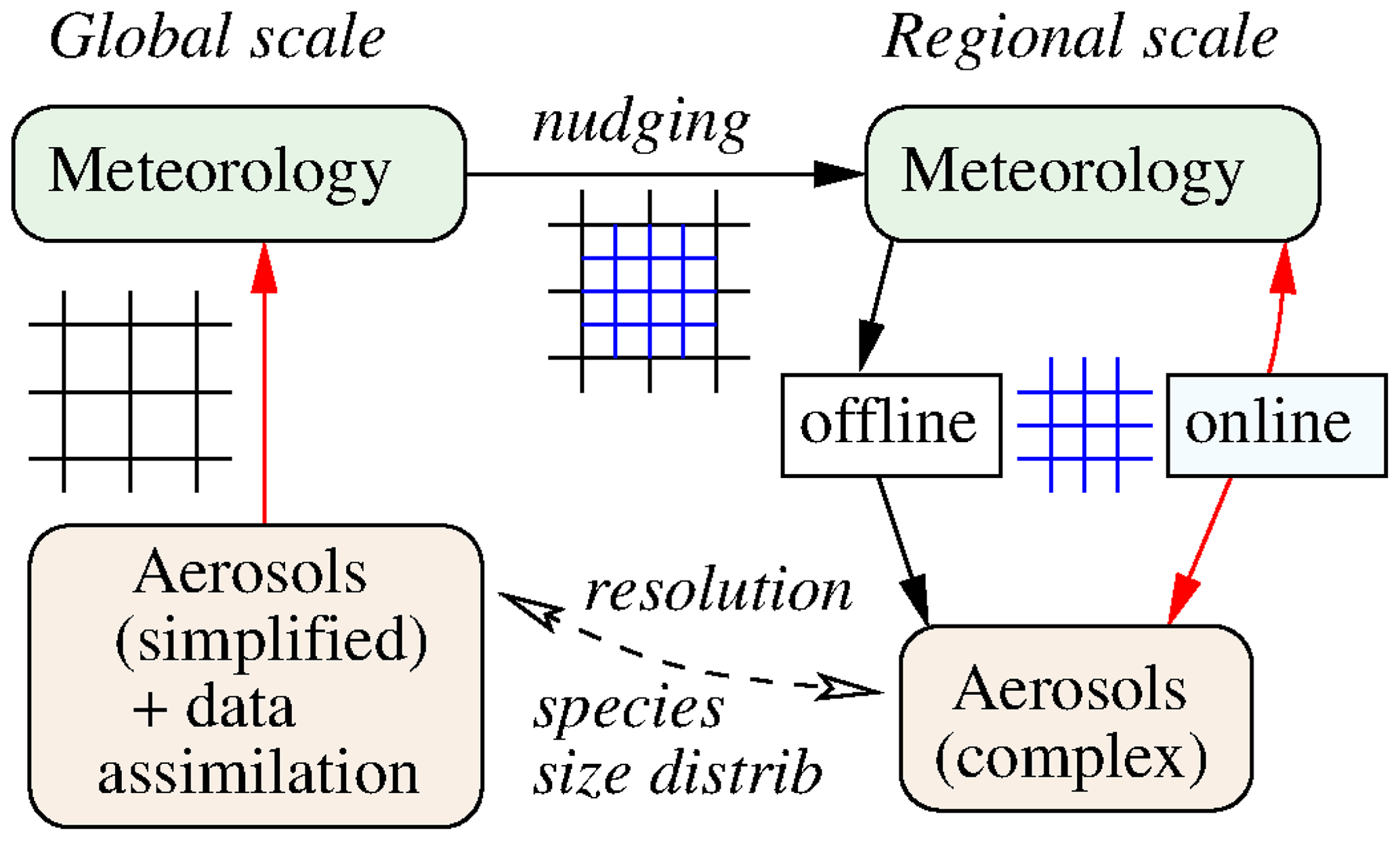
Figure 1 The paradox of a regional model nudged by a global model. The global model performs a meteorological simulation, which generally includes aerosol climatology to take into account the direct and indirect effects of aerosols. If the simulation is a reanalysis, there may also be data assimilation, such as the optical thickness estimated from satellite observations. But the overall simulation will have included aerosols in the meteorological calculation. This global simulation will serve as a forcing for the regional simulation. The regional meteorological model will serve as a forcing tool or will be coupled to the CTM calculating aerosols. Aerosols are also taken into account, but at a different resolution. The black grid is the global model, and the blue grid is the regional model. The dotted arrow indicates that aerosols may not be the same species or have the same size distribution, depending on the chemistry-transport and climatology models used.

The effect of nudging on the modelling of regional meteorology is paradoxical: nudging improves the realism of simulations by forcing them to stay close to the observed reality, but this is achieved by introducing unrealistic inconsistencies between the dynamics and the physics of the model, thereby possibly limiting or distorting (Lin et al., 2016) our understanding of processes by dampening the effect of model parameterizations. As presented in Fig. 1, the global scale (used for nudging) and the regional scale are supposed to represent the same physical reality, but they rely on different aerosol forcings, spatial resolutions and parameterizations, thereby leading to divergent meteorologies for the same location. We therefore have two processes acting in parallel: data assimilation on large-scale fields (global forcing, for example) and meteorological and chemical-transport coupling at a smaller scale. This paradox leaves the modeller with a methodological choice: either avoid nudging and let model physics operate freely, ensuring consistency between the physics and the dynamics, or use nudging and ensure that the model stays close enough to observations, but at the cost of introducing inconsistencies between the dynamics and the physics.

This methodological alternative has already been reported in regional and global climate modelling, particularly when discussing the good use of nudging to evaluate model sensitivity to a forcing or to parameterization choices. It is already well known in that field that the use of nudging techniques, while indispensable for the representation of individual events in a realistic way, can dampen the response of models to other effects such as air–sea coupling (Berthou et al., 2016) or convective parameterizations (Song et al., 2011). While it improves the representation of individual events, nudging forces a model to reproduce a large-scale variability that is not necessarily in equilibrium with its physical parameterizations, thereby introducing inconsistency between the dynamics and physics (Pohl and Crétat, 2013). On the bright side, nudging reduces the internal variability in the model and therefore the spread between several different realizations, such as the sensitivity studies performed to evaluate the effect of a particular process or parameterization, permitting the robust detection of such effects from shorter simulations (Sun et al., 2019). For example, Kooperman et al. (2012) show that, by attenuating the “natural variability” between two sensitivity simulations, nudging permits the isolation of the direct effect of a physical process from natural variability. In summary, the effect of nudging on sensitivity studies is twofold. On the one hand, it dampens the effect of a change in processes or parameterizations (Song et al., 2011; Pohl and Crétat, 2013; Lin et al., 2016; Berthou et al., 2016) and introduces inconsistencies between the dynamics and the physics (Pohl and Crétat, 2013; Lin et al., 2016); on the other hand, it strongly reduces the internal (chaotic) variability of meteorology in the numerical simulations and thereby permits sensitivity effects to be observed in a more robust way (Kooperman et al., 2012; Lin et al., 2016; Sun et al., 2019), even in relatively short simulations, as is the case in the present study.

The effect of nudging on regional simulation has been studied mainly in relation to meteorological variables such as temperature and precipitation. Using the WRF (Weather Research and Forecasting) model (Powers et al., 2017), Glisan et al. (2013) studied the effect of nudging on arctic temperature and precipitation. They showed that the results are not sensitive to the strength of the nudging. Spero et al. (2014) proposed changes in the spectral nudging to improve clouds, radiation and precipitation in their WRF simulations. He et al. (2017) studied the climatological timescale; more specifically, they studied possible changes in temperature due to the combined effects of large-scale forcing and regional aerosol–radiation interactions. They concluded that it is possible and realistic to use nudging in aerosol radiative effect studies, but with increased caution as the spatial scale decreases. Rizza et al. (2020) explored the sensitivity of the WRF model to various configurations, including spectral nudging. They compared their results to meteorological (wind, temperature) surface measurements and concluded that there is no benefit from nudging the meteorology inside the boundary layer.

Studies of the impact of this methodology on pollutant concentrations, the focus of the present study, are very rare. In these cases, they are more dedicated to regional climate (trends, long-term scenarios) than to regional atmospheric pollution cases. One of the first studies was done by (Hogrefe et al., 2015), who performed simulation tests in the framework of the AQMEII2 (Air Quality Model Evaluation International Initiative) project and showed that nudging reduces the bias for temperature with or without aerosol effects. They showed that, for temperature, the effect of nudging is larger than the effect of the feedback of aerosols on meteorology. The same question arises in He et al. (2017) about the relative impact of temperature nudging compared to aerosol radiative effects. They showed that nudging has less effect than aerosol–radiation interactions at global and regional scales but could be more important at the local scale.

In the present study, we will focus on regional-scale modelling and the impact of spectral nudging on both the meteorology and pollutant concentrations for a limited temporal scale. Simulations of the same case are carried out to evaluate the weight of nudging on cloud–radiative–aerosol interactions. The key question here is to determine whether nudging or coupling is most important for pollutant concentrations on a regional scale and how nudging and coupling interact. Even if they are not the same kind of processes and not directly comparable, they are often “free parameters” that are up to the user, making it important to understand well their relative weights for modelled surface concentrations of pollutants. Section 2 describes the models used and the simulation configurations. Section 3 presents the results of various simulations performed with the WRF and CHIMERE models. Section 4 presents refined results in the case of online coupling. Finally, conclusions are presented.

2 The modelling system

The two models used in this study are WRF 3.7.1 (Powers et al., 2017) and CHIMERE 2020r3 (Menut et al., 2021). The simulations are done over a single domain with a horizontal resolution of 50 km × 50 km, as presented in Fig. 2. Simulations are performed from 1 July to 31 August 2022. This corresponds to the same domain and the same period as presented in Menut et al. (2023).

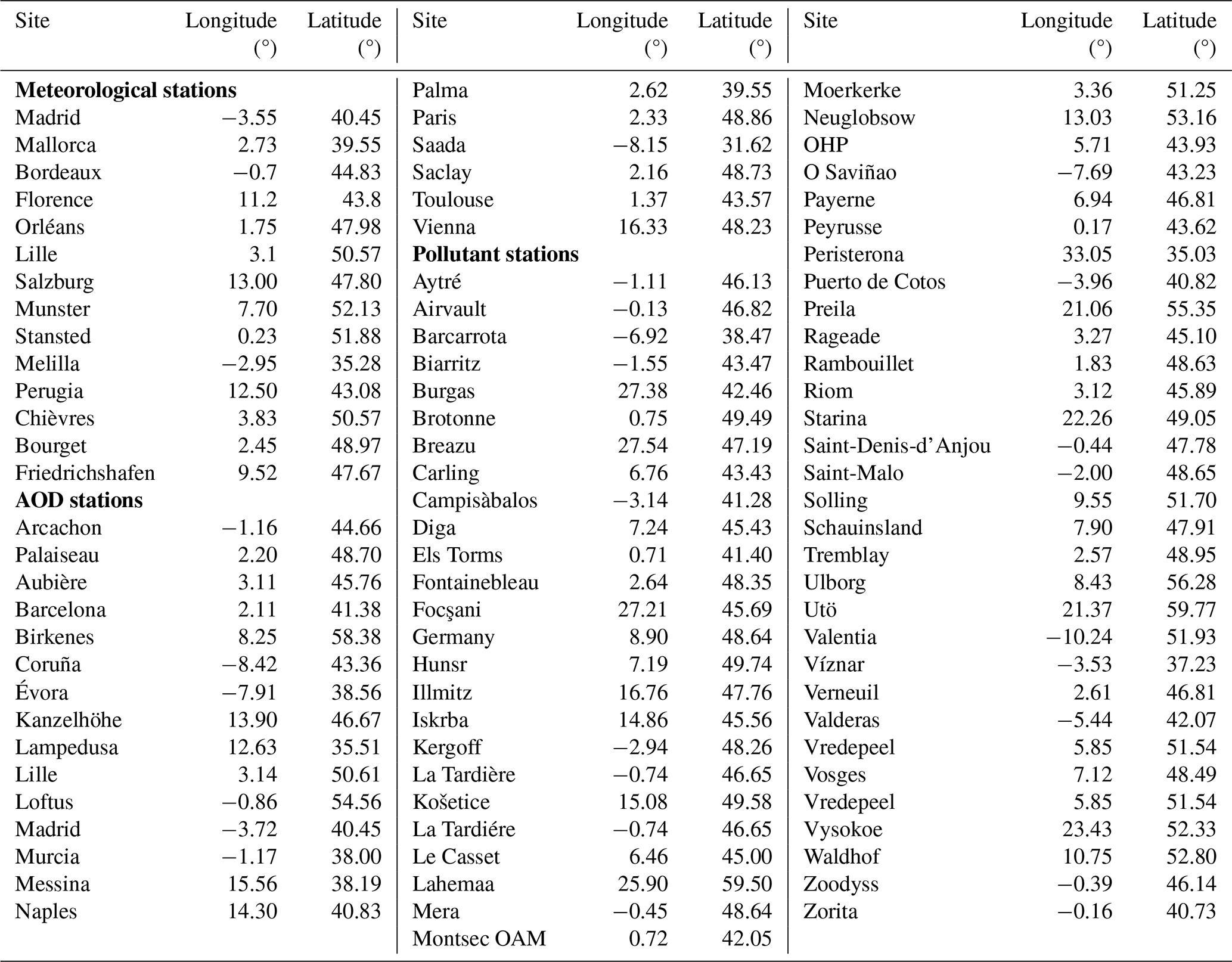
Figure 2 Maps of measurement stations, including meteorological (blue points), EEA (European Environment Agency; green points) and AERONET (AErosol RObotic NETwork; red points) stations. A zoom of western Europe, where stations are more numerous, is presented. For readability, only two letters of each name are reported. The complete list of stations, along with their coordinates, is presented in Table A1. Meteorological stations are represented with blue squares, AERONET stations with red diamonds and pollution stations with green circles.

The model was configured with and without spectral nudging in WRF and with and without taking into account direct and indirect aerosol effects. This leads to four different simulations, as explained in Table 1.

Table 1 Simulations performed for this study.

2.1 The WRF model set-up

2.1.1 The main schemes used

Many physical schemes are available in WRF, and many studies have quantified the impact of several combinations on the results (Cohen et al., 2015). The model is used with a constant horizontal resolution of 50 km × 50 km on a horizontal grid of 103 × 106 cells and with 28 vertical levels from the surface to 50 hPa. The single-moment 5-class microphysics scheme is used, allowing for mixed-phase processes and supercooled water (Hong et al., 2004). The radiation scheme is the RRTMG (Rapid Radiative Transfer Model for general circulation models) scheme with the McICA (Monte Carlo Independent Column Approximation) random cloud overlap method (Mlawer et al., 1997). The surface layer scheme is based on Monin–Obukhov theory with a Carlson–Boland viscous sub-layer. The surface physics is calculated using the Noah land surface model scheme with four soil temperature and moisture layers (Chen and Dudhia, 2001). The planetary boundary layer physics is processed using the Yonsei University scheme (Hong et al., 2006), and the cumulus parameterization uses the ensemble scheme of Grell and Dévényi (2002).

2.1.2 The nudging choices

Several studies have been devoted to the comparison between grid and spectral nudging (Liu et al., 2012; Vincent and Hahmann, 2015; Ma et al., 2016; Zittis et al., 2018). The two approaches have strengths and weaknesses. Grid nudging has the characteristic that it is applied over all grid cells, while spectral nudging is applied only in zonal and meridional directions and only for some predefined wavenumbers. Grid nudging seems more appropriate for precipitation intensity (Ma et al., 2016). On the other hand, spectral nudging is less intrusive at a small scale and gives the regional model more freedom than large-scale forcing. One can also note that spectral nudging has a greater numerical cost than grid nudging (Zittis et al., 2018). In this study, we prefer to use spectral nudging to get more variability at the regional scale.

Usually, spectral nudging is applied to four meteorological variables: the wind components u and v, the temperature, and the geopotential height. The nudging of specific humidity is avoided, as it is considered to be badly represented at the largest scale by the forcing model (Heikkila et al., 2010; Otte et al., 2012). The nudging of water vapour (or moisture) is also avoided by Liu et al. (2012), considering that this variable has no large-scale features that are as strong as those of the other meteorological fields. In addition, nudging temperature and humidity at the same time may produce inconsistencies (Sun et al., 2019). However, Spero et al. (2014) consider that not nudging this variable may be the reason for the overestimation of precipitation when using spectral nudging compared to grid nudging. They considered that nudging moisture guarantees that thermodynamical fields (the potential temperature and the water mixing ratio) are treated consistently. But this nudging should only be done below the tropopause, as excessively large values occur in the stratosphere with some global models. They also note that for moisture, the best coefficient is 4.5 × 10⁻⁵ s⁻¹ to be consistent with the input data fields that have a frequency of 6 h. Using a lower value (3 × 10⁻⁴ s⁻¹ and therefore 1 h) induces an overprediction of precipitation. For all these studies, there is no nudging in the boundary layer.

An important parameter is the nudging coefficient (in s⁻¹), denoted g. This coefficient may have different values depending on the meteorological variable: the wind components u and v (coefficient: guv), the temperature (gt), and the water vapour (gq). When using spectral nudging in WRF, it is also possible to nudge geopotential height perturbations (gph). With the WRF model, the default value is equal to 0.0003 s⁻¹, corresponding to a value found in many studies such as Liu et al. (2012), Otte et al. (2012), Ma et al. (2016), Gomez and Miguez-Macho (2017), Zittis et al. (2018), and Huang et al. (2021). Some other studies, such as Choi et al. (2009), Cha et al. (2011), Glisan et al. (2013), Spero et al. (2014), He et al. (2017) and Spero et al. (2018), have performed sensitivity experiments to quantify the impact of this value on the results, and no significant impact was found. This value corresponds to a 1 h frequency for the use of nudging and is highly representative of the large-scale fields used as forcing as well as the frequency of the data used for the analysis of the global fields. In this study, this value is used for all simulations with nudging. The wind components, the potential temperature perturbation and the water vapour mixing ratio are nudged using spectral nudging with a coefficient g of 0.0003 s⁻¹. There is no nudging in the planetary boundary layer (PBL).

The calculation frequency is set to have active nudging every time step. The wavenumbers are calculated with the hypothesis that features greater than 1000 km in size are sufficiently well resolved in a global model (Gomez and Miguez-Macho, 2017). Then, the following equation is applied (for the x direction, for example):

$$\begin{array}{}\text{(1)}& x_{\mathrm{wn}}=\mathrm{int}\left({\displaystyle \frac{\mathrm{\Delta }x\times N_x}{R}}\right),\end{array}$$

where Δx is the horizontal resolution (in metres), N_x is the number of grid cells and R is the Rossby radius value (da Silva and de Camargo, 2018; Mai et al., 2020). For this study and a horizontal resolution of 50 km (in both the zonal and meridional directions), this leads to a wavenumber of x_wn=5. The same value is found for y_wn, as the grid size is the same and the number of cells is similar in the two directions.

2.2 The CHIMERE model configuration

This v2020r3 version of CHIMERE is currently the latest-distributed one and is designed to either take into account the direct and indirect effects of aerosols on cloud and radiation (the online mode) or not (the offline mode). The way these effects are taken into account is described in Briant et al. (2017) (for the direct effect) and Tuccella et al. (2019) (for the indirect effect). Mainly, the direct effect corresponds to the attenuation of radiation by aerosol layers, and the indirect effect corresponds to cloud formation caused by the presence of fine particles. When used with the meteorological model WRF, CHIMERE and WRF are coupled using the OASIS–MCT (Ocean Atmosphere Sea Ice Soil–Model Coupling Toolkit) coupler. In offline mode, WRF sends hourly meteorological fields for chemistry transport to CHIMERE, and CHIMERE sends aerosols and aerosol optical depth fields to WRF for the radiation attenuation and microphysics in WRF.

The model configuration is exactly the same as in Menut et al. (2023): it includes emissions from anthropogenic, biogenic, sea-salt, biomass-burning, lightning NO_x and mineral dust sources. It also includes gaseous and aerosol chemistry for tens of chemical species. For gases, the MELCHIOR 2 scheme is used as described in Menut et al. (2013) and Mailler et al. (2017). For aerosols, 10 bins from 0.01 to 40 µm are used. The anthropogenic emissions are those from CAMS (Granier et al., 2019). The dry deposition is modelled following the Zhang et al. (2001) scheme, and the wet deposition follows Wang et al. (2014). The biomass-burning emissions are those from CAMS as described in Kaiser et al. (2012) but with an additional term, burned area, as presented in Menut et al. (2022, 2023); this is designed to calculate the impact of fires on additional mineral dust emissions, change of LAI (leaf area index) and biogenic emissions. The mineral dust emissions are parameterized following Alfaro and Gomes (2001) and modified following Menut et al. (2005). Vertical fluxes of emission are calculated such that the size distribution of the emission depends on the magnitude of the friction velocity, the soil distribution and its mineral characteristics. The humidity is taken into account via the soil moisture with the parameterization from Fecan et al. (1999). The effects of precipitation and soil recovery on emissions are also taken into account following Mailler et al. (2017).

2.3 The measurement data

For the surface pollutant concentrations, the European Environment Agency (EEA, https://www.eea.europa.eu, last access: 3 May 2024) provides a full set of hourly data for particulate matter (PM_2.5 and PM₁₀), ozone (O₃) and nitrogen dioxide (NO₂) from a large number of stations in western Europe. Only urban, rural and suburban background stations are used in this study, considering that the industrial and traffic ones provide inadequate spatial representativity for the present model outputs. For the aerosol optical depth (AOD) and the Ångström exponent (ANG), AErosol RObotic NETwork (AERONET, https://aeronet.gsfc.nasa.gov/, last access: 3 May 2024) level 1.5 measurements are used (Holben et al., 2001). The AOD at a wavelength of λ=675 nm is averaged daily and compared to daily averaged modelled values. The available measurement values are averaged over a 24 h period from midnight to midnight. Only the corresponding values are considered with the model. For the 2 m temperature and 10 m wind speed, the measurements are provided by the weather information website of the University of Wyoming (UWYO) (http://www.weather.uwyo.edu/, last access: 3 May 2024). Data are provided as integer values, restraining the accuracy of the comparison to the model results. A complete list of measurement stations is displayed in Table A1. Maps of the stations for which the measurements were used are presented in Fig. 2.

The results will be presented in two different formats: general statistics (to show the trend of impacts on simulated values) and examples of time series and maps (to illustrate these statistics more precisely). The measurement stations chosen as examples were selected for their representativeness in relation to the other stations as well as for their geographical positions in relation to the processes studied.

3 Results

3.1 Statistical scores

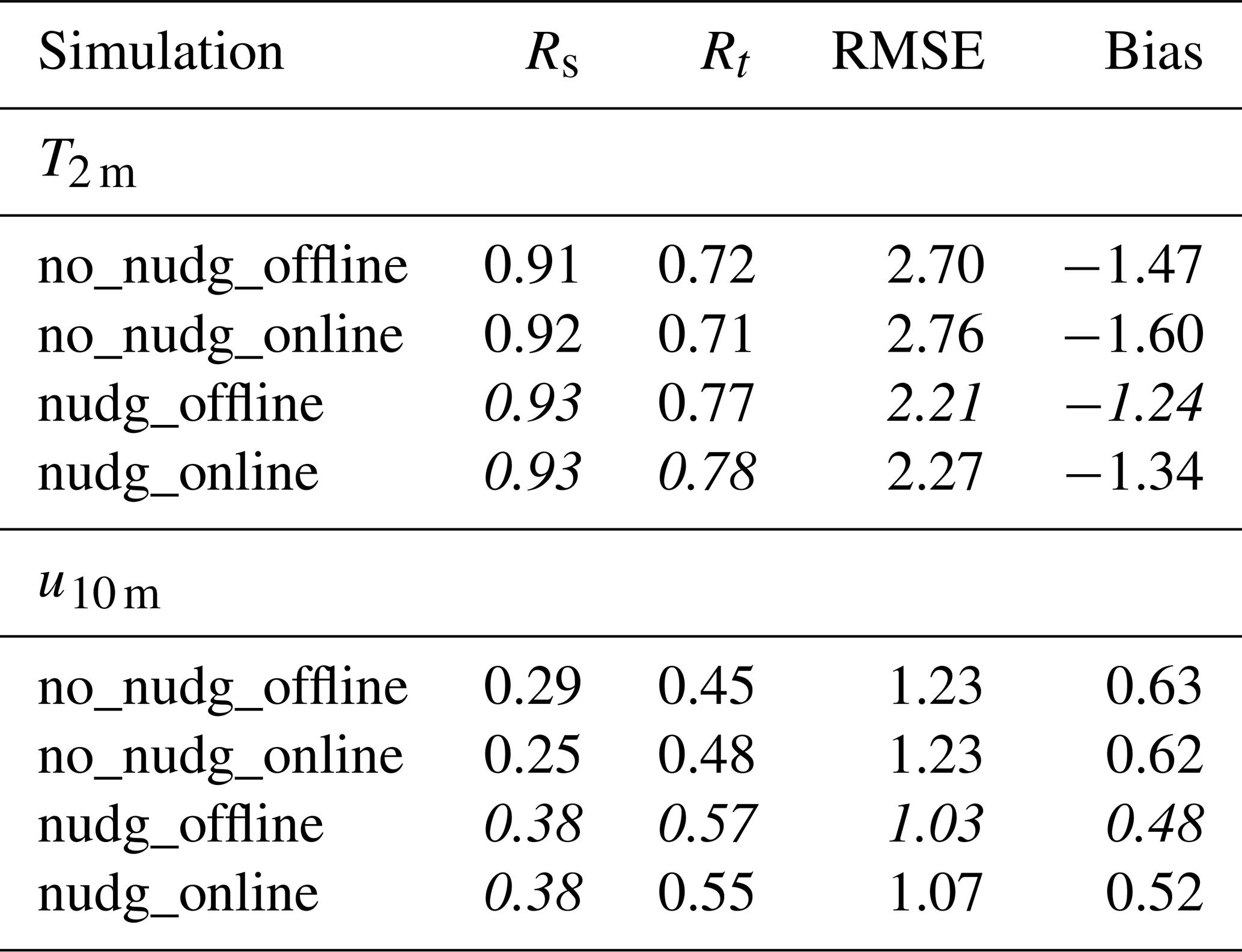
For meteorological variables such as 2 m temperature (°C) and 10 m wind speed (m s⁻¹), measured by surface stations, statistical scores are presented in Table 2. These scores are calculated using all hourly data from the meteorological stations. They are defined as follows.

The variables O_t and M_t stand for the observed and modelled values, respectively, at time t. The mean value $\stackrel{\mathrm{‾}}{X_N}$ is defined as

$$\begin{array}{}\text{(2)}& \stackrel{\mathrm{‾}}{X_N}={\displaystyle \frac{\mathrm{1}}{N}}\sum _{t=\mathrm{1}}^N{X}_t,\end{array}$$

where N is the total number of hours of the simulation. To quantify the temporal variability, the Pearson product moment correlation coefficient R is calculated as

$$\begin{array}{}\text{(3)}& R={\displaystyle \frac{\frac{\mathrm{1}}{N}{\sum }_{t=\mathrm{1}}^N(M_t-\stackrel{\mathrm{‾}}{M_t})\times (O_t-\stackrel{\mathrm{‾}}{O_t})}{\sqrt{\frac{\mathrm{1}}{N}{\sum }_{t=\mathrm{1}}^N(M_t-\stackrel{\mathrm{‾}}{M_t}{)}^{\mathrm{2}}\times \frac{\mathrm{1}}{N}{\sum }_{t=\mathrm{1}}^N(O_t-\stackrel{\mathrm{‾}}{O_t}{)}^{\mathrm{2}}}}}.\end{array}$$

The spatial correlation, denoted R_s, uses the same formula type, except that it is calculated from the temporal mean averaged values of the observations and the model for each location where observations are available.

$$\begin{array}{}\text{(4)}& R_{\mathrm{s}}={\displaystyle \frac{{\sum }_{i=\mathrm{1}}^I(\stackrel{\mathrm{‾}}{M_i}-\stackrel{\mathrm{‾}}{\stackrel{\mathrm{‾}}{M}})(\stackrel{\mathrm{‾}}{O_i}-\stackrel{\mathrm{‾}}{\stackrel{\mathrm{‾}}{O}})}{\sqrt{{\sum }_{i=\mathrm{1}}^I(\stackrel{\mathrm{‾}}{M_i}-\stackrel{\mathrm{‾}}{\stackrel{\mathrm{‾}}{M}}{)}^{\mathrm{2}}{\sum }_{i=\mathrm{1}}^I(\stackrel{\mathrm{‾}}{O_i}-\stackrel{\mathrm{‾}}{\stackrel{\mathrm{‾}}{O}}{)}^{\mathrm{2}}}}},\end{array}$$

where I is the number of stations. The root mean square error (RMSE) is expressed as

$$\begin{array}{}\text{(5)}& \mathrm{RMSE}=\sqrt{{\displaystyle \frac{\mathrm{1}}{T}}\sum _{t=\mathrm{1}}^T{\left(O_{t,i}-M_{t,i}\right)}^{\mathrm{2}}}.\end{array}$$

To quantify the mean differences between the several leads, the bias is also quantified as

$$\begin{array}{}\text{(6)}& \mathrm{bias}={\displaystyle \frac{\mathrm{1}}{N}}\sum _{t=\mathrm{1}}^N(M_t-O_t).\end{array}$$

For these two variables, 2 m temperature (T_2 m) and 10 m wind speed (u_10 m), the best scores are obtained for the simulations with spectral nudging, but not systematically for the simulation with the coupling. The scores reflect the spatial and temporal representativeness of the variables. Temperature at 2 m is more representative of the large scale than wind speed at 10 m, which is more local. Given the resolution of the model, the wind scores are logically lower. Globally, it is noticeable that for meteorological variables, the nudging configurations always have better statistical scores, which is logical given that these variables are directly nudged. The offline configuration gives the best results, even if differences between online and offline are low.

Table 2 Statistical scores for 2 m temperature (K) and 10 m wind speed (m s⁻¹). Scores are calculated for all stations and over the entire modelled period (July and August 2022). The best score values are in italic.

For surface concentrations and optical properties, results are presented in Table 3 as statistical scores in order to quantify the relative impacts of the coupling and the spectral nudging. These scores are calculated by comparison between the modelled outputs and the measured surface concentrations and optical properties for the corresponding location and hour.

Table 3 Statistical scores for the surface ozone, PM_2.5 and PM₁₀ (µg m⁻³) concentrations; AOD (no dim.); and Ångström exponent (no dim.) in comparison with EEA and AERONET measurements and the four simulations. Scores are calculated for all stations and over the entire modelled period (July and August 2022). The best score values are in italic.

For the surface concentrations, the three modelled chemical concentrations (ozone, PM_2.5 and PM₁₀) are compared against measurements. The spatial correlation is always the same or better when the nudging is used. In the case of nudging, the spatial correlation is more or less the same for the simulation with or without coupling. For the temporal correlation, the same type of result is observed: statistical scores are systematically better with the nudging. The impact of the coupling is less important, and the scores are lower with and without the coupling. The RMSE is systematically lower with the nudging as well as the bias for the three variables.

For the optical properties, the conclusion is close to that for the surface concentrations. The statistical scores are systematically better with the nudging than without it. This is true for the AOD and the Ångström exponent. The spatial and temporal correlations are better, and the bias and the RMSE are reduced. For the surface concentrations, there is no clear impact of the use of the coupling (with direct and indirect effects) on the scores. The correlations are better in the case of no nudging and less good with nudging. However, the impact remains low.

The conclusion based on these results is that the differences between the simulations with and without coupling are not significant. But the differences depending on whether nudging is used are significant, and the use of nudging always improves the simulation scores for all variables, the spatial and temporal correlations, the bias, and the RMSE.

3.2 Time series of meteorological variables

As this study is based on nudging and coupling, it is important to compare the impacts of the several simulation configurations on the meteorological variables. Simulation results are compared with surface measurements from meteorological stations in Europe and Africa. A list of the stations used is displayed in Table A1. Here, we present examples for two stations in France, Orléans and Bordeaux, located close to the studied fires. Bordeaux was the closest station to the studied Landes fires and was directly under the fire plume. Orléans is located at 400 km to the northeast of Bordeaux but was also under the fire plume. Time series of daily averaged 2 m temperature and 10 m wind speed for these two stations in France are presented in Fig. 3. Note that this type of comparison was also made for many other stations, and the results were of the same kind. For the 2 m temperature, simulation results are close to the measurements during the whole period. The simulations are grouped into two sets: with and without nudging. The simulations with and without coupling are very close. One can note that lower values around 20 July are correctly modelled for Orléans by the nudging simulations, whereas the no-nudging simulations overestimate the values. Other differences are noted for the period from 10 to 20 August: the simulations differ in both temperature and wind speed.

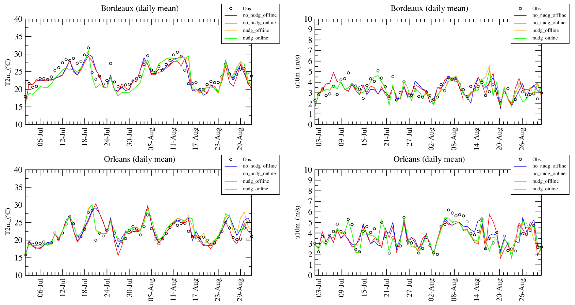
Figure 3 Time series of daily mean 2 m temperature (°C) and 10 m wind speed (m s⁻¹) for the stations of Bordeaux and Orléans over the months of July and August 2022.

To better discuss these differences observed in August, a temporal zoom is done for 13 to 20 August, and the results are displayed in Fig. 4. Data and model outputs at an hourly frequency are now presented. For the temperature, the first 3 d shows a large diurnal cycle with values ranging from 18 to 40 °C, in contrast to the last 3 d, which shows a reduced diurnal cycle with values of between 16 and 25 °C. The model is able to follow this weather change except around the day of 15 August, when the model continues to have a large diurnal cycle, which is not observed. Except for 15 August in Bordeaux and 16 August in Orléans, the four simulations provide close values of temperature. This is not the case for the 10 m wind speed, where all four simulations provide very different values for the 6 consecutive days. For example, in Orléans, the variability of the wind speed is important; it ranges from 1 to 10 m s⁻¹, depending on the simulation configuration. Finally, for the whole modelled period, there is no evidence as to which simulation best reproduces the observations, but the statistical scores (Table 2) show that the simulations with nudging perform better.

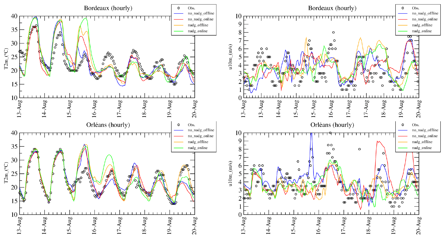
Figure 4 Time series of hourly 2 m temperature (°C) and 10 m wind speed (m s⁻¹) for the stations of Bordeaux and Orléans for the period from 13 to 20 August 2022.

3.3 Time series of surface concentrations

In order to have a more detailed look at the results, time series of surface concentrations of ozone and PM_2.5 (in µg m⁻³) are presented in Fig. 5. Results are presented for two sites, Biarritz and Fontainebleau. As already discussed in Menut et al. (2023), Biarritz, located in the south of France, was under the plumes from biomass burning that came from Spain in mid-July and mid-August 2022. Fontainebleau, near Paris, was not close to the Landes fires but was under their plume between 12 and 18 July 2022.

Figure 5 Daily mean surface concentrations (in µg m⁻³) in Biarritz (a, c) and Fontainebleau (b, d) for ozone (O₃) and particulate matter with a mean mass median diameter less than 2.5 µm (PM_2.5).

In Biarritz, two main peaks are recorded at the same time for ozone and PM_2.5 on 16 July and 14 August 2022. For the four simulations, the magnitudes and the variability of the modelled concentrations are realistic and comparable to the surface observations. It is difficult to disentangle the several simulations and to diagnose the best scores without statistical calculations. The time series exhibits notable day-to-day variability for all simulations. A third peak is modelled but not measured on 30 July, but only for the configurations without nudging. With nudging, the model removes this peak and is therefore closer to the observations.

In Fontainebleau, the time variability is not the same for ozone and PM₁₀. But, for all simulations, the model is close to the observations and the day-to-day variability is reproduced well. For ozone, the largest differences are seen for the simulation nudg_online, with the largest values occurring on 13 and 19 July, representing the best correspondence to the measurements. For the same simulation, on 21 July, the PM₁₀ concentrations are lower, making them closer to the observations, than in the other simulations. Note that a peak is observed for ozone around 13 August, but this is not modelled by any of the four simulations. This probably corresponds to long-range transport and an error in the synoptic flow and hence long-range ozone transport. This is because the configurations tested correspond to meteorological perturbations on a regional scale and within the study area. The fact that none of the four configurations simulate this peak shows that it is not due to a local or regional event.

In conclusion, the model simulations with nudging enable some non-observed peaks to be avoided (such as those for ozone in Biarritz and PM₁₀ in Fontainebleau). The four simulations all have a large day-to-day variability, and there is no systematic bias between the simulations which could indicate a persistent effect of a process. The four simulations are comparable to the observations; there is no configuration that is very false. This means that the use of nudging and the use of coupling are not mutually exclusive and that using spectral nudging outside of the boundary layer probably does not interfere with coupling, which has more a local or regional effect.

3.4 Time series of optical depth

Time series of daily mean values are presented in Fig. 6 for the Ångström exponent (ANG) and aerosol optical depth (AOD) in Birkenes, Barcelona and Toulouse. We can expect greater differences between simulations than for surface concentrations. ANG and AOD incorporate changes throughout the simulated atmospheric column, the troposphere. Therefore, we take into account more possible changes between simulations, including changes on larger spatial scales, such as in long-range aerosol transport.

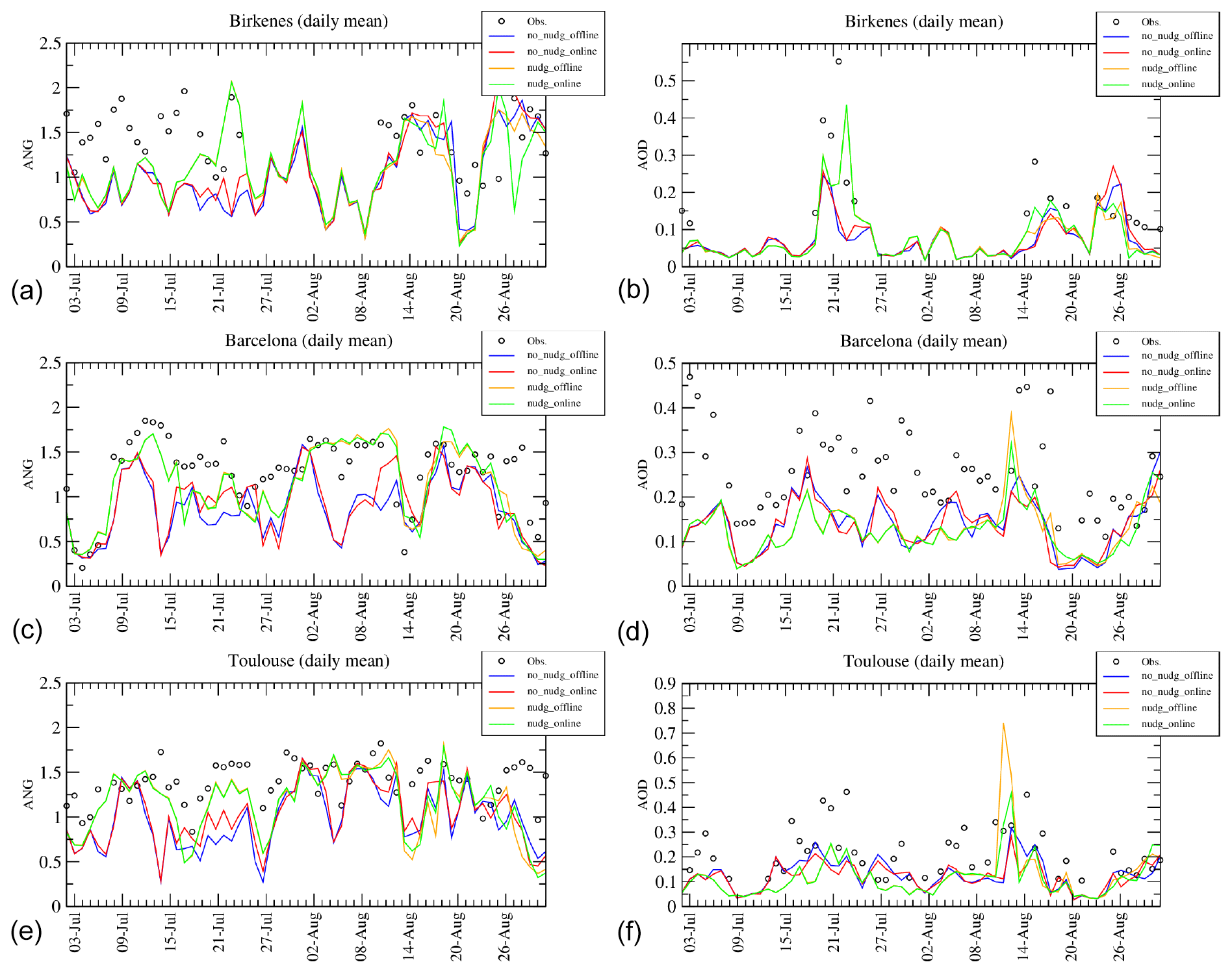
Figure 6 Time series of the Ångström exponent (ANG, a, c, e) and aerosol optical depth (AOD, b, d, f) in Birkenes, Barcelona and Toulouse.

For the three sites and the two variables, one observes the same as for the surface concentrations. The two simulations with no nudging are close, and the two simulations with nudging are also close. But the simulations with no nudging are very different from the simulations with nudging. This means that the direct or indirect effects are less dominant than nudging.

In Birkenes, the ANG time series shows that the model overestimates the aerosol size by simulating coarse-mode aerosols (low values of ANG) when the measurements are between 1.5 and 2 and thus representative of the fine mode. This bias is mitigated by simulations with nudging, which better simulate the fine mode around 21 July. The simulations with nudging also better simulate a notable AOD peak on this day, with observed values around 0.5. For the rest of the period, the four simulations are relatively close, for both ANG and AOD. As Birkenes is close to desert areas where dust is emitted, the bias is reduced with the nudg_online configuration because these two forcings are able to better represent the wind speed and direction.

In Barcelona, the best capacity of the model to retrieve the observed ANG and AOD is observed for the simulations with nudging. This is clear for the period from 9 to 16 July, when only the nudged simulations are able to simulate the high ANG values. The nudging will help the regional model to have a better wind speed. The mineral dust scheme used is the one from Alfaro and Gomes (2001). This scheme has wind-speed-dependent dust emission, both for the intensity of the emitted flux and for the size distribution. By changing the wind speed, the size distribution of dust is changed for all the aerosols. The same behaviour is observed during the period from 2 to 10 August, when the model correctly calculates an ANG of around 1.5 but the non-nudged simulation calculates low values (between 0.5 and 1). One can note that the simulations without nudging show non-negligible differences between them. For the AOD, the four simulations underestimate the values compared to the observations. For 13 August, the two configurations with nudging are able to simulate the observed peak in AOD, in contrast to the simulations without nudging.

In Toulouse, the ANG values are between 1 and 1.5, indicating relatively small particles. The day-to-day variability is close to that in Barcelona, with the same peaks occurring during the same periods. All model configurations are close, except during the period from 13 to 19 July for ANG: only the configurations with nudging are able to simulate high values of ANG that are close to the measurements. Also, for AOD, only the nudged configurations are able to reproduce a peak representative of the measurements.

In conclusion, simulations with nudging give consistently better results, especially when ANG or AOD peaks are observed. Differences can be seen between simulations without nudging and those with or without coupling. For simulations with nudging, there are no real differences between simulations with and without coupling. So, we can see that nudging gives better scores but leaves less variability than for the online configurations.

3.5 Time-averaged maps

Time-averaged maps are presented in this section. The averaging period is 1 month from 1 to 31 August 2022. Differences are calculated between these averaged maps. Since there are four different configurations, the following differences are calculated:

• (nonudg_online − nonudg_offline) – impact of the coupling in the case of no spectral nudging

• (nudg_online − nudg_offline) – impact of the coupling in the case of spectral nudging

• (nudg_offline − nonudg_offline) – impact of the nudging with no direct/indirect effects

• (nudg_online − nonudg_online) – impact of the nudging with direct/indirect effects.

Figure 7 Differences in the vertically averaged water vapour mixing ratio (g kg⁻¹) time-averaged over the period from 1 to 31 August 2022.

Results are presented in Fig. 7 for the water vapour mixing ratio. This variable is particularly important for the radiative transfer (specifically at night). Water vapour as a radiative forcer contributes significantly to the greenhouse effect: between 35 % and 65 % for clear-sky conditions and between 65 % and 85 % for a cloudy day, as reported in Bessagnet et al. (2020) and references therein. The water vapour concentration fluctuates regionally and locally, as shown in particular in the land-to-water transition bands and in mountainous areas. In these latter regions, at night, the long-wave radiation is one of the most important variables governing the radiative budget. A change of water mixing ratio initiated at valley bottoms by small motions immediately modifies the radiative balance. First of all, we note that the spatial structures of the difference values differ between the four figures. The top figures show the impact of coupling, while the bottom figures show the impact of nudging. Depending on the location, the differences may be negative or positive. Large spatial structures exist, showing that changes may affect large areas or may be transported. There is no systematic location for the negative or positive changes. The impact of the coupling is less important than the impact of nudging. The spatial structures are negative or positive and are not linked to vegetation or mountainous areas or urbanized areas. The positive changes are more important than the negative ones.

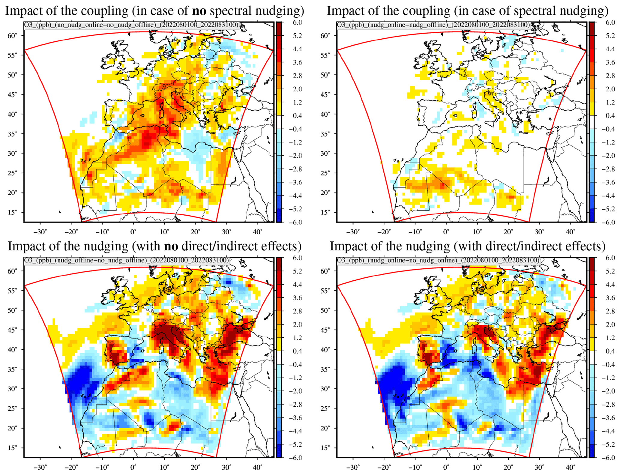
Figure 8 Differences in surface ozone concentrations time-averaged over the period from 1 to 31 August 2022.

The same difference calculations are done for surface ozone concentrations (Fig. 8). Just as for the water vapour, the differences are more significant with nudging. The spatial structure is not directly comparable between the two variables. This is normal, as we are representing a surface quantity – a secondary pollutant that is potentially produced and transported in a completely different way to water vapour (which is presented vertically integrated). For the effects of coupling, the differences are more significant and positive over North Africa, with a maximum of +3 µg m⁻³. Over western Europe, the differences alternate between negative and positive values but never exceed ±1 µg m⁻³. Non-zero differences are spatially very rare, and the majority of the differences are below the low value of ±0.4 µg m⁻³. Figure 8 for nudg_online also shows much larger differences over the whole simulation domain. Positive and negative differences can occur over sea or over land; no specific patterns are visible. Depending on the location and averaged over a month, the differences due to nudging can reach ±6 µg m⁻³ for surface ozone concentrations.

The previous results are summarized in Fig. 9 as distributions of the values displayed in the previous maps. The comparison of all differences presented as distributions enables us to see the spread of these differences over the domain. For all variables, the peak in the distribution is seen for the differences (nudg_online − nudg_offline, green curve) and (nonudg_online − nonudg_offline, red curve). These curves correspond to the simulations of the variability due to the coupling. The peaks indicate that these model configurations are those with the smallest differences. In addition, one can see that the differences are smaller with the green curve (nudging) than the red curve (no nudging). This means that the nudging reduces the variability of the simulations when comparing simulations with and without coupling. The two other types of differences, (nudg_offline − nonudg_offline, blue curve) and (nudg_online − nonudg_online, orange curve), express the sensitivity of the model results to the nudging. In this case, the peak representing small differences is reduced, and numerous large differences are calculated, both negative and positive. It means that, independently of the coupling, the nudging causes many more differences than the coupling. This is the case for meteorological variables and surface pollutant concentrations.

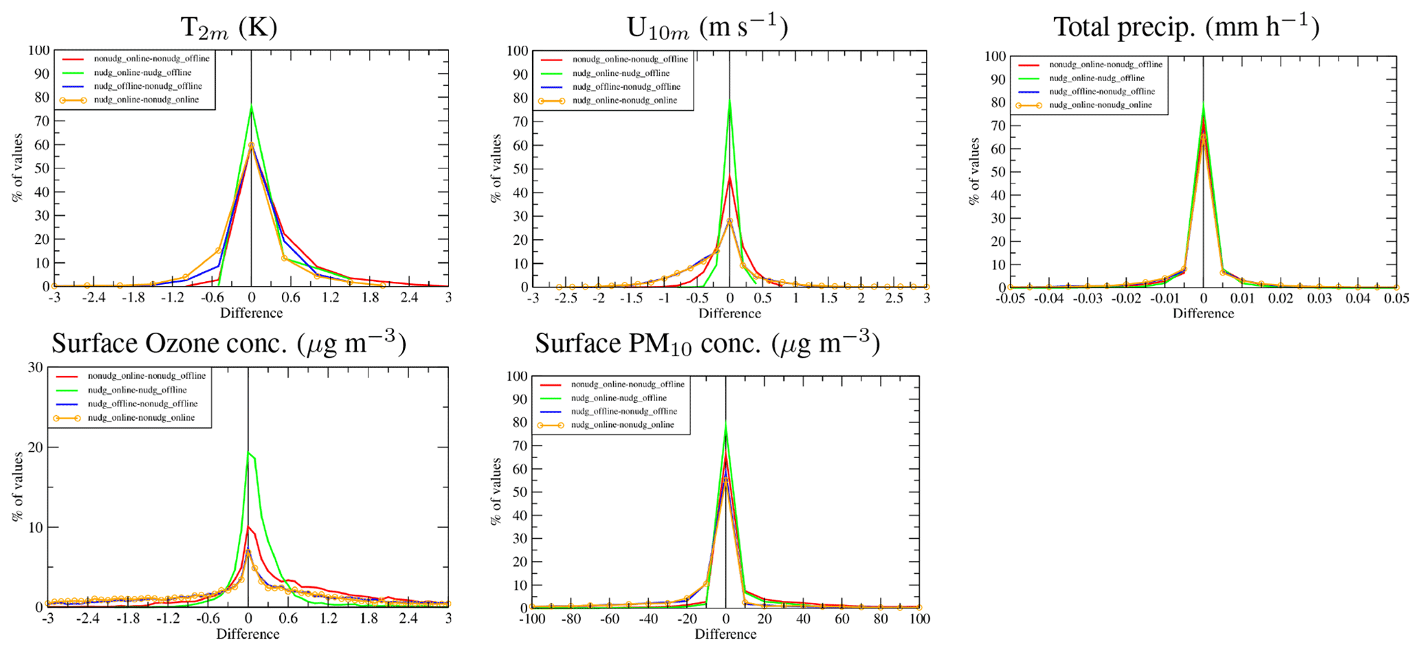
Figure 9 Histogram of difference values that are time-averaged over the period from 1 to 31 August 2022.

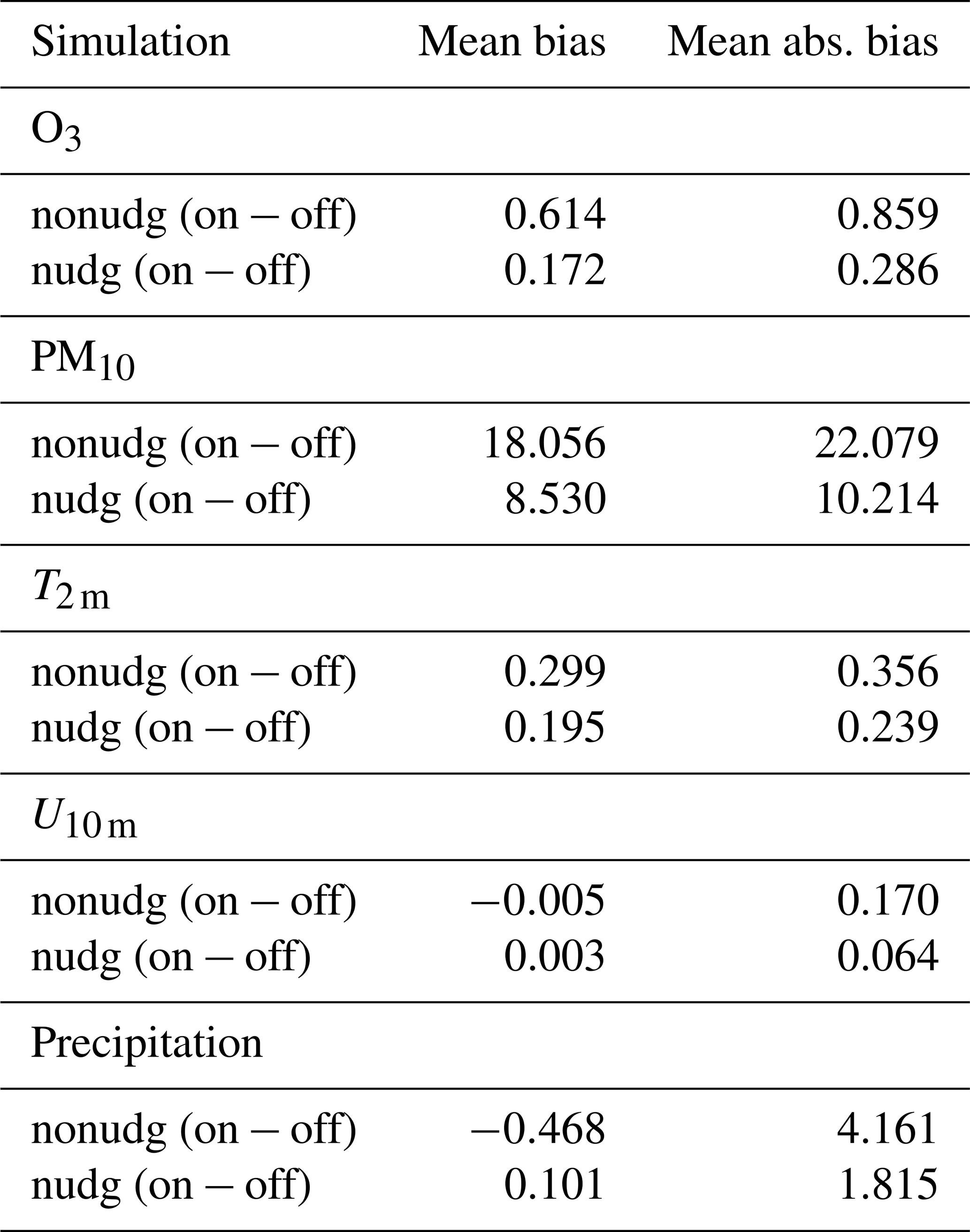
Additionally, results are also synthesized as mean averaged differences extracted from the maps of differences presented in the previous figures. The results are shown in Table 4, and the goal is to try to extract information about the variability of the coupling in the case of nudging and in the case of no nudging. The time series and the distributions previously showed that the differences between the offline and online simulations are larger when there is no nudging than when there is nudging. The values in the table quantify this. The mean differences are first calculated using the sign values. But, as the distributions showed that there is large variability between negative and positive differences over the entire domain, we also add the mean differences calculated using the absolute values of the differences.

For each variable, it is interesting to compare the two lines: in each case, the difference is between offline and online simulations, and this difference is given for the case of no nudging and the case of nudging. For all variables, the differences obtained with no nudging are larger than the differences obtained with nudging. This is observed for both the simple differences and the differences calculated with the absolute values. This means that the nudging reduces the variability of the simulations when they are online compared to those offline.

Table 4 Mean averaged differences for the entire month of August 2022 over the whole domain. Mean differences are calculated with either the signed values or the absolute values in order to avoid the effect of the presence of negative and positive values, which could reduce the mean average.

3.6 Vertical cross-sections

Another point of view for the meteorological variables is displayed in Fig. 10 with temperature vertical cross-sections. Values are displayed for latitudes from 15 to 55° N and the iso-longitude value of 5° E. This longitude corresponds to the middle of France, the place where the fire plumes passed over the Landes (where the emissions were), and Belgium and Germany (after transport). Data are time-averaged between 10 August 00:00 UTC and 12 August 00:00 UTC. For the impact of the coupling, changes are more significant in the case of no spectral nudging. The largest differences occur between 5000 and 8000 m, where changes range approximately between ±1.5 °C. For the impact of the nudging, the changes are much larger, but similar values are seen with or without online effects. The changes are not located in the same place as for the impact of the coupling: negative values of $\approx -\mathrm{1.8}$ °C occur where they were positive in the other case. Large positive values occur in the boundary layer and in the free troposphere.

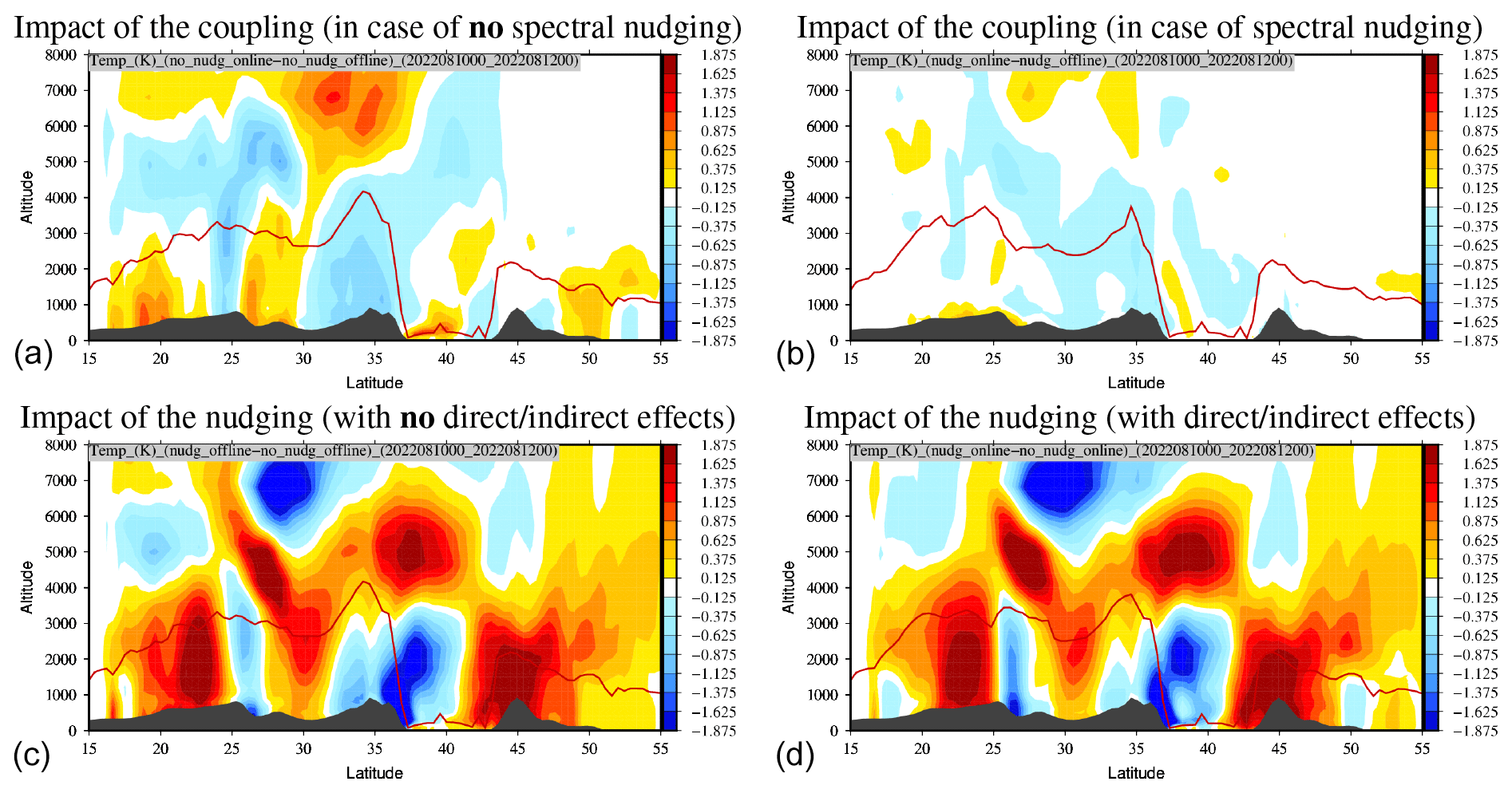
Figure 10 Vertical cross-section of differences in temperature (°C) between spectral nudging and no spectral nudging and between coupling and no coupling. The data were time-averaged over the period from 10 to 12 August 2022. The boundary layer height (m) superimposed in red corresponds to simulation X if the difference is X − Y.

Vertical cross-sections of ozone concentrations at a constant longitude are displayed in Fig. 11 (for the same place and period as in the previous figure). Just as for the temperature, changes are greater in the case of the impact of the nudging than in the case of the impact of the coupling. Changes occur mostly above the boundary layer and are both negative and positive, with an amplitude range of ±20 µg m⁻³. The vertical structures are different than those for temperature, which shows that there is no direct link between the two variables. The smallest changes occur in the case of coupling and spectral nudging, the most realistic configuration, where ozone varies by less than ±10 µg m⁻³ across the whole modelled atmospheric column, with very low values occurring close to the surface.

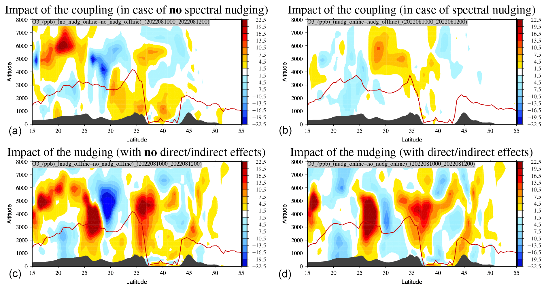
Figure 11 Vertical cross-section of differences in O₃ (µg m⁻³) between spectral nudging and no spectral nudging and between coupling and no coupling. The data were time-averaged over the period from 10 to 12 August 2022. The red line represents the boundary layer height (m) of the simulation (a) if the difference is (a)–(b).

Vertical cross-sections are also presented for PM₁₀ concentrations in Fig. 12. Differences between the four configurations are smaller than for the previously studied variables. The largest differences are still seen for the impact of the nudging. Absolute differences are limited to the boundary layer, with maximum difference values of ±300 µg m⁻³. The location shows that these differences are mainly at latitudes lower than 30° N, indicating desert areas, so these differences are driven by mineral dust concentrations. Negative values are found at altitudes between 1000 and 3000 m and above the Mediterranean Sea (latitude 40° N), showing that the nudging reduces the concentrations. These negative values are collocated with an increase in ozone, which can be explained by the fact that less aerosol means higher radiative fluxes and therefore more photochemistry.

Figure 12 Vertical cross-section of differences in PM₁₀ (µg m⁻³) between spectral nudging and no spectral nudging and between coupling and no coupling. The data were time-averaged over the period from 10 to 12 August 2022. The red line represents the boundary layer height (m) of the simulation (a) if the difference is (a)–(b).

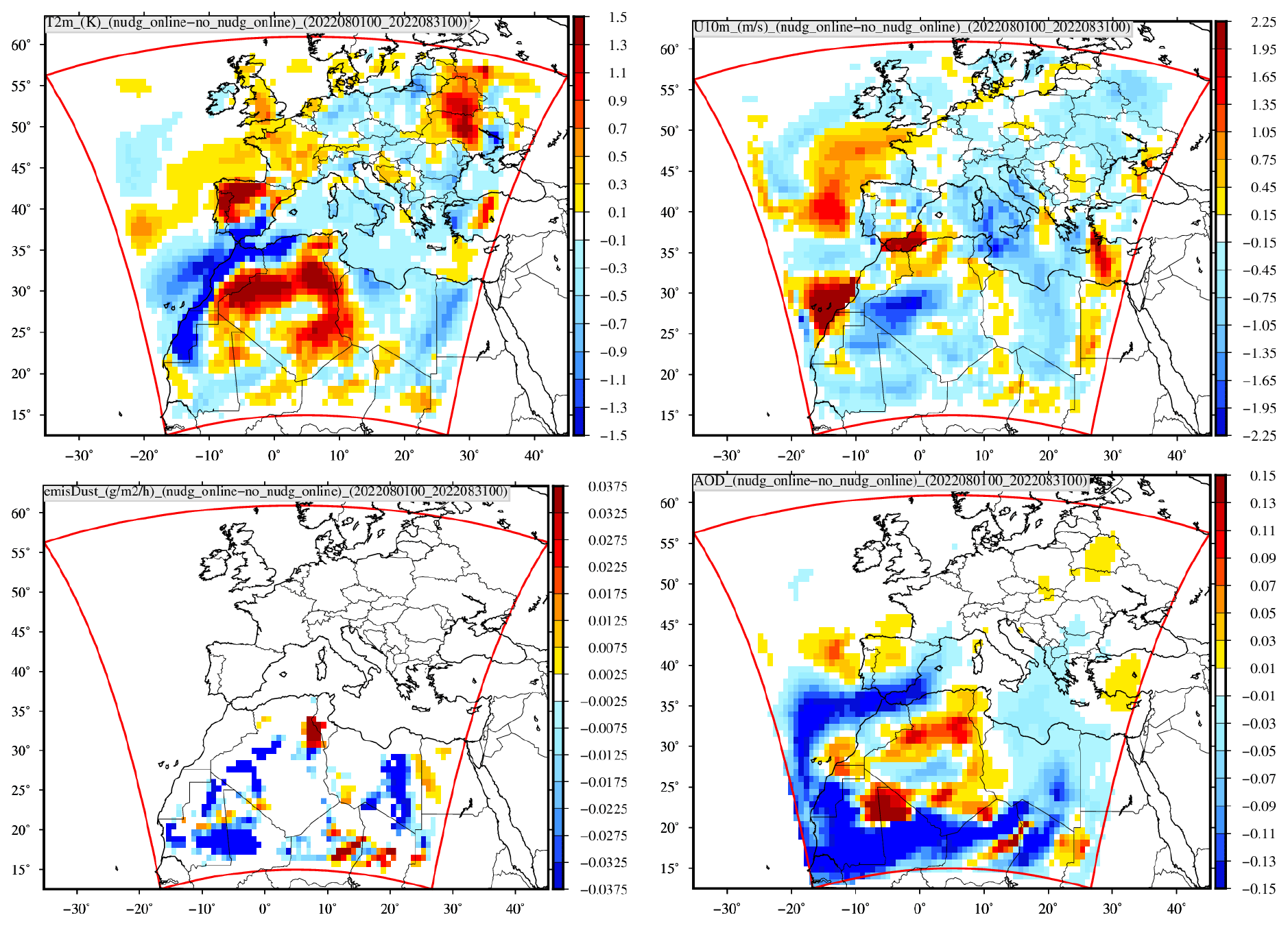
Figure 13 Differences in 2 m temperature (K), 10 m wind speed (m s⁻¹), mineral dust emissions (g m⁻² h⁻¹) and AOD (no dim.) between the spectral-nudging and no-spectral-nudging cases. The data were obtained in online coupling mode and were time-averaged over the period from 1 to 31 August 2022.

4 Online coupling: impact of the spectral nudging

It has already been shown that the impact of nudging is far greater than that of online vs. offline coupling. In the following, we will therefore only present results for the online configuration, which corresponds to the most realistic processes. Only the differences between the cases with spectral nudging and no spectral nudging will be calculated and presented here.

Results are presented in Fig. 13 for the 2 m temperature (K), 10 m wind speed (m s⁻¹), mineral dust emissions (g m⁻² h⁻¹) and AOD (no dim.) between the spectral-nudging and no-spectral-nudging cases, where the data were obtained in online coupling mode and were time-averaged over the period from 1 to 31 August 2022. Just as for the previously presented variables, there are no systematic spatial patterns or coherent structures. This effect is always due to the fact that the results are presented as averages over a month, incorporating local changes and their transport. But the important task is to assess their magnitudes in terms of differences.

For temperature, the differences are both negative and positive and can reach ±1.5 K. For the 10 m wind speed, these differences are mainly negative (a reduction in wind), except over the sea, where local positive maxima can reach 2 m s⁻¹. Due to the geophysics equations, there is no reason to have a direct link between temperature and wind speed at the surface when the nudging is used: the differences are not due to the geophysics but to the forcing exerted by the large scale on the regional scale by the two different models. For mineral dust emissions, the differences are localized to where these emissions occur, i.e. mainly in North Africa. The main trend is for negative differences, showing that, on average, nudging tends to reduce these emissions. The differences in AOD represent a synthesis of the previous differences. This variable represents the aerosol load in the atmosphere and therefore reflects changes in temperature and wind speed; it also therefore reflects dust emissions, their concentrations and therefore their optical thickness. There are wide spatial variations in AOD, with large positive structures over Africa but also large negative structures over the southwestern part of the domain, including a maritime area. The differences are large: around ±0.15. For the large area in the southwest of the domain where AOD is lower, this could be mostly due to the difference in the 10 m wind speed, which is also negative. Since the AOD is representative of the whole atmospheric column and the 10 m wind speed is only representative of the surface, no further link between the differences for these two variables can be established.

5 Conclusions

In this study, we have investigated the impact of the spectral nudging and coupling (aerosol cloud radiation) on regional simulations of atmospheric pollutants. These two processes are able to modify the meteorology, but not necessarily in the same way. Their effects can be double-counted or contradictory; however, in both cases, they should better represent the reality we try to simulate.

To quantify this impact, we carried out four simulations, each lasting 2 months (during the summer of 2022) and covering Europe and part of Africa. These four simulations were combinations with or without nudging and with or without coupling. The results show, first of all, that the four simulations differ from one another. For the pollutants studied (O₃, PM₁₀) and for AOD, and in comparison with measurements, the simulations with nudging give the best results, showing that, as expected, applying nudging leads to simulation outputs that are closer to the observed data. At this point, the conclusions of the present study align with what is already known for climate models and extend them to chemistry-transport modelling.

We also observed that the use of nudging reduces the sensitivity of the outputs to the model configuration (in our case, the application of online coupling). As a consequence, the effect of coupling on the meteorological variables is smaller when nudging is applied, which was expected from previous studies (Pohl and Crétat, 2013), but we saw that the effect of coupling on the concentrations of gas-phase and particulate species is also smaller when nudging is applied (Table 4). In our case, the sensitivity of the model outputs to coupling is reduced by a factor ranging from 30 % to 70 %, depending on the variables. While this might suggest that nudging could lead to an underestimation of the model sensitivity to coupling, it has been shown in climate modelling that applying nudging also gives more significance to the simulated sensitivity by dampening the internal variability of the meteorological model.

The results of our study, summarized in Table 4, can be interpreted as ranges of the sensitivity of the key variables in meteorology and chemistry-transport models to aerosol–meteorology feedback, with the sensitivity in the presence (or absence) of nudging giving an lower (or upper) boundary for the sensitivity of each variable to aerosol–meteorology feedback. The sensitivity determined in the absence of nudging includes not only the effect of the feedbacks themselves but also that of the internal variability of the meteorological model, while the sensitivity in the presence of nudging essentially includes the effect of the feedbacks, which is possibly dampened by nudging. For example, in the present study, the sensitivity of PM₁₀ concentration to these feedbacks ranges between 10 and 22 µg m⁻³, the sensitivity of ozone to these feedbacks ranges between 0.29 and 0.862 µg m⁻³, and the sensitivity of 2 m temperature to these feedbacks ranges between 0.24 and 0.36 K. This conclusion is of course limited to the models used; to the simulation domain and period studied; and to the parameters chosen, particularly the nudging constants. An important outcome of this study is the fact that the use of nudging and coupling options can have counterintuitive impacts when CTMs are used to analyse the impact of emission reduction scenarios. For instance, it is very important to keep in mind that in the case of an online meteorological system, concentrations change not only because emissions change but also because of feedbacks of aerosols to meteorology. In a follow-up to this study, the simulations should be repeated with nested domains to address one other dimension of the problem: the impact of the horizontal resolution.

Appendix A: List of measurement stations

Table A1 Names and locations of measurement stations used in this study.