Emission ensemble approach to improve the development of multi-scale emission inventories

Many studies have shown that emission inventories are one of the inputs with the most critical influences on the results of air quality modelling. Comparing emission inventories among themselves is, therefore, essential to build confidence in emission estimates. In this work, we extend the approach of Thunis et al. (2022) to compare emission inventories by building a benchmark that serves as a reference for comparisons. This benchmark is an ensemble that is based on three state-of-the-art EU-wide inventories: CAMS-REG, EMEP and EDGAR. The ensemble-based methodology screens differences between inventories and the ensemble. It excludes differences that are not relevant and identifies among the remaining ones those that need special attention. We applied the ensemble-based screening to both an EU-wide and a local (Poland) inventory.

The EU-wide analysis highlighted a large number of inconsistencies. While the origin of some differences between EDGAR and the ensemble can be identified, their magnitude remains to be explained. These differences mostly occur for SO₂ (sulfur oxides), PM (particulate matter) and NMVOC (non-methane volatile organic carbon) for the industrial and residential sectors and reach a factor of 10 in some instances. Spatial inconsistencies mostly occur for the industry and other sectors.

At the local scale, inconsistencies relate mostly to differences in country sectorial shares that result from different sectors/activities being accounted for in the two types of inventories. This is explained by the fact that some emission sources are omitted in the local inventory due to a lack of appropriate geographically allocated activity data. We identified sectors and pollutants for which discussion between local and EU-wide emission compilers would be needed in order to reduce the magnitude of the observed differences (e.g. in the residential and industrial sectors).

The ensemble-based screening proved to be a useful approach to spot inconsistencies by reducing the number of necessary inventory comparisons. With the progressive resolution of inconsistencies and associated inventory improvements, the ensemble will improve. In this sense, we see the ensemble as a useful tool to motivate the community around a single common benchmark and monitor progress towards the improvement of regionally and locally developed emission inventories.

1 Introduction

Many studies have shown that emission inventories are one of the inputs with the most critical influences on the results of air quality modelling (Kryza et al., 2015; Zhang et al., 2015). Even more concerning, certain studies have shown that important uncertainties affect emission inventories, which may impeach conclusions based on air quality model results (Trombetti et al., 2018; Markakis et al., 2015). These uncertainties result from the need to compile a wide variety of information to develop an emission inventory. For the many pollutants and activity sectors to cover, the spatial and temporal distribution of emissions is typically based on proxies that can be estimated through different methods.

In Thunis et al. (2022), we showed that comparing emission inventories is an effective way to detect inconsistencies when differences are very large. A methodology was designed to compare two emission inventories, one against the other. This methodology identifies disparities between the two inventories by assessing country totals, their sectorial share and the proportion of the country emissions attributed to the urban areas. In this work, we adhere to the same principle of analysing differences while introducing a novel ensemble concept to facilitate the simultaneous comparison of a larger number of inventories.

Ensemble modelling has widely been used in climate (Kotlarski et al., 2014) and air quality modelling fields throughout the world (Stevenson et al., 2006; Vautard et al., 2009; Marécal et al., 2015; Brasseur et al., 2019) as they generally provide better and more robust results. While in some instances reference values (e.g. measurements) exist against which models can be compared, this is unfortunately not the case for emissions, and, hence, the emission ensemble is not necessarily better than any of its members. The emission ensemble is therefore not a more accurate inventory. This is, however, not an issue as the ensemble is used here as a common benchmark for comparison. Moreover, our focus is on the differences between emission estimates rather than on their absolute values, for which accuracy and robustness are of secondary importance. The underlying concept is that above a certain threshold, the differences are so large that one or both inventories can be considered wrong. The choice of this vocabulary, i.e. wrong, is intentional and is meant here to foster the process of reviewing the data when differences exceed a given threshold. In other words, a difference by a factor of 100 between inventories for a given sector/pollutant most likely reveals one or more significant errors (or inconsistencies), which are relatively straightforward to identify and must be addressed in either one or both inventories. The methodology screens differences between inventories, excludes differences that are not relevant (i.e. large differences on low emission values are disregarded) and identifies among the remaining ones those that need special attention.

In addition to this key advantage, several other objectives are pursued by introducing the ensemble for EU-wide emission inventories, namely (1) to create a unique common benchmark to monitor and quantify the current level of agreement among the ensemble members, (2) to identify and characterise the largest mismatches in terms of pollutant or sector among them, (3) to foster interactions between EU-wide emission inventory developers around identified inconsistencies, and (4) to allow for comparing additional inventories (e.g. bottom-up inventories) with the ensemble. A comparison of the ensemble with local (intended here as national or sub-national) inventories can indeed be helpful as they are independent estimates, since methods are based on local knowledge and understanding of the activities and processes that result in emissions.

This work is structured as follows. In Sect. 2, we review the screening methodology proposed in Thunis et al. (2022) and discuss the construction of the ensemble in the frame of this screening approach. In Sect. 3, we apply the ensemble-based screening approach to one EU-wide inventory, whereas in Sect. 4 we illustrate how this ensemble can then be compared to local inventories in a bilateral manner. For the latter, a local inventory developed for Poland is used. In Sect. 5, we discuss the main findings from both types of comparisons and conclude in Sect. 6.

2 Description of the methodology

2.1 Overview of the screening methodology

In this section, we provide a brief summary of the screening method detailed in Thunis et al. (2022). The approach aims at comparing two emission inventories over a series of urban areas over which the consistency is assessed for all sectors and pollutants. Based on gridded annual emissions detailed in terms of pollutants (“p”) and sectors of activity (“s”), the data required for each pollutant and sector (p–s couple) are twofold and consist of (1) emissions aggregated over specific urban areas (lowercase notation e_p,s) and (2) country-scale emissions (uppercase notation E_p,s).

The consistency between emissions in both inventories is assessed around three aspects: (1) the total pollutant emissions assigned at country level; (2) the way these country emissions are distributed across sector; and (3) the way country emissions are distributed spatially and, therefore, allocated to main urban areas. To address these three aspects, we decompose the ratio of the known pollutant–sector emissions for each city as follows:

$$\begin{array}{}\text{(1)}& {\displaystyle \frac{e_{\mathrm{p},\mathrm{s}}^{\mathrm{1}}}{e_{\mathrm{p},\mathrm{s}}^{\mathrm{2}}}}={\displaystyle \frac{\frac{e_{\mathrm{p},\mathrm{s}}^{\mathrm{1}}}{E_{\mathrm{p},\mathrm{s}}^{\mathrm{1}}}}{\frac{e_{\mathrm{p},\mathrm{s}}^{\mathrm{2}}}{E_{\mathrm{p},\mathrm{s}}^{\mathrm{2}}}}}\cdot {\displaystyle \frac{\frac{E_{\mathrm{p},\mathrm{s}}^{\mathrm{1}}}{{\overline{E}}_{\mathrm{p}}^{\mathrm{1}}}}{\frac{E_{\mathrm{p},\mathrm{s}}^{\mathrm{2}}}{{\overline{E}}_{\mathrm{p}}^{\mathrm{2}}}}}\cdot {\displaystyle \frac{{\overline{E}}_{\mathrm{p}}^{\mathrm{1}}}{{\overline{E}}_{\mathrm{p}}^{\mathrm{2}}}},\end{array}$$

where ${\overline{E}}_{\mathrm{p}}$ represents the country-scale emissions summed over all sectors for a given pollutant. Superscripts refer to the two inventories used for the screening. Equation (1) is an identity where all terms are known from input quantities, i.e. the city and country-scale emissions detailed in terms of pollutants and sectors. The three terms on the right-hand side of the identity provide information on spatial distribution (FAS, focus area share), on the country sectorial share (LSS, large-scale sectorial share) and on the country pollutant totals (LPT, large-scale pollutant total).

For convenience, we rewrite Eq. (2) in logarithm form as

$$\begin{array}{}\text{(2)}& \log \left({\displaystyle \frac{e_{\mathrm{p},\mathrm{s}}^{\mathrm{1}}}{e_{\mathrm{p},\mathrm{s}}^{\mathrm{2}}}}\right)=\log \left({\displaystyle \frac{\frac{e_{\mathrm{p},\mathrm{s}}^{\mathrm{1}}}{E_{\mathrm{p},\mathrm{s}}^{\mathrm{1}}}}{\frac{e_{\mathrm{p},\mathrm{s}}^{\mathrm{2}}}{E_{\mathrm{p},\mathrm{s}}^{\mathrm{2}}}}}\right)+\log \left({\displaystyle \frac{\frac{E_{\mathrm{p},\mathrm{s}}^{\mathrm{1}}}{{\overline{E}}_{\mathrm{p}}^{\mathrm{1}}}}{\frac{E_{\mathrm{p},\mathrm{s}}^{\mathrm{2}}}{{\overline{E}}_{\mathrm{p}}^{\mathrm{2}}}}}\right)+\log \left({\displaystyle \frac{{\overline{E}}_{\mathrm{p}}^{\mathrm{1}}}{{\overline{E}}_{\mathrm{p}}^{\mathrm{2}}}}\right),\end{array}$$

which can be rewritten as Eq. (3) with simplified notations as

$$\begin{array}{}\text{(3)}& \widehat{e}=\widehat{\text{FAS}}+\widehat{\text{LSS}}+\widehat{\text{LPT}},\end{array}$$

where the hat symbol ( $\widehat{}$ ) indicates that quantities are expressed as logarithmic ratios. These three quantities form the basis of the screening methodology and serve as input information for a graphical representation that facilitates the interpretation of the results.

As the number of p–s points under screening, equivalent to the product of the number of pollutants and sectors further multiplied by the number of urban areas (i.e. $N\times N_{\mathrm{p}}\times N_{\mathrm{s}}$), may become overwhelming, we adopt a series of steps to concentrate the screening on priority aspects. First, we restrict the screening to emissions that are relevant, i.e. large enough. As shown in Thunis et al. (2022), this exclusion step leads to eliminating a large fraction of the p–s couples from the screening process (between 80 % and 90 %). Second, we flag, among the remaining emissions, only those for which inventory emission ratios are larger than a given threshold (β_t).

When differences are small, it is not possible to tell whether they originate from methodological choices or from errors. We refer to these small differences as “uncertainty”. Although very large differences may result from methodological choices as well (e.g. inclusion or not of particulate matter condensable emissions for the residential sector), they are more likely to be associated with errors. Given the magnitude of the differences, it will in most cases be possible to identify one best value out of the two inventory estimates, even though the true emissions are unknown. These large differences are named “inconsistencies”. In the proposed screening methodology, a β_t of 2 (free parameter) is introduced to distinguish inconsistencies from uncertainties.

As a follow-up step, all p–s couples that remain after the relevance test and inconsistency detection steps (${\mathit{\beta }}_{\mathrm{p},\mathrm{s}}>{\mathit{\beta }}_{\mathrm{t}}$) are used to calculate an emission consistency indicator (ECI) as follows:

$$\begin{array}{}\text{(4)}& \text{ECI}={\displaystyle \frac{\log \left({\mathit{\beta }}_{\mathrm{p},\mathrm{s}}\right)}{\log \left({\mathit{\beta }}_{\mathrm{t}}\right)}}.\end{array}$$

The ECI quantifies the maximum difference among all relevant p–s, normalised by the inconsistency threshold. It therefore quantifies the ratio between the maximum inconsistency and the assumed level of uncertainty. A value of an ECI less than 1 means that all differences are considered as uncertainty (in other words, none of the inventory can be identified as best performing). Together with the ECI, which quantifies this maximum difference, we associate the percentage of inconsistent p–s with respect to the total number of relevant data, in order to provide information on the number of detected inconsistencies.

Finally, we prioritise inconsistencies following the LPT–LSS–FAS hierarchy. In other words, if large-scale inconsistencies are spotted for LPT, they are flagged as the priority, regardless of the magnitude of inconsistencies calculated for LSS and/or FAS. If no inconsistency is flagged for LPT, the same holds for LSS regardless of the level of inconsistency calculated for FAS. Consequently, the inconsistency flagged as the priority might not be the largest inconsistency. This hierarchy is motivated by the fact that addressing large-scale inconsistencies will lead to potentially resolving several issues at once (e.g. all urban areas within a given country). Inconsistencies are counted not only when the individual terms in Eq. (3) are larger than β_t but also when the indicator sums (i.e. $\widehat{\text{FAS}}+\widehat{\text{LSS}}+\widehat{\text{LPT}}$, $\widehat{\text{LSS}}+\widehat{\text{LPT}}$) exceed this threshold.

It is important to note that the method follows a bottom-up approach; i.e. we assess the three types of inconsistencies for each city, pollutant and sector. This means that the same LPT inconsistency is counted for all cities within a given country or for all sectors for a given pollutant. Similarly, an LSS inconsistency is counted for each city belonging to the same country. While this might be seen as double counting of some inconsistencies, the approach allows for the comparison of local- vs. country-scale indicators.

2.2 Construction of an ensemble as reference

This work aims at applying a novel ensemble concept to extend the methodology from Thunis et al. (2022) to several inventories. The ensemble is calculated from EU-wide inventories that have been developed and regularly updated over several years within the EU¹. While either the mean or the median of these inventories could be used to calculate the ensemble, we choose to use the median as it has been shown to be a more robust indicator compared to the mean (Riccio et al., 2007). Indeed, if one of the inventories is a strong outlier (i.e. much larger or much smaller values), then the mean would be strongly influenced by these extreme values and would differ from the values of most of the inventories. On the other hand, the median is not affected by extreme values and therefore takes a value closer to the values taken by most of the inventories. It therefore remains further away from the outliers, which become easier to identify.

In this work, the ensemble is created from three state-of-the-art EU-wide inventories: CAMS-REG (Copernicus Atmosphere Monitoring Service-regional; all other abbreviations can be found in “Appendix A: list of abbreviations”), EMEP and EDGAR.

EDGAR is a comprehensive global emission inventory providing country and sector-specific greenhouse gas and air pollutant emissions from 1970 until present. EDGAR is becoming a global reference for anthropogenic emissions, in particular contributing to the IPCC-AR6 (Sixth Assessment Report) and to the annual UNEP emissions gap reports (UNEP, 2023) tackling global climate change issues. In the context of air pollution, EDGAR is also widely used by air quality modellers, playing an important role as gap-filling inventory in the Hemispheric Transport of Air Pollution mosaic compilation. Emissions are computed using a consistent methodology for all world countries, following the IPCC guidelines (IPCC, 2006, 2019) and the EMEP/EEA guidebook (EMEP/EEA; 2016, 2019) for greenhouse gases (GHGs) and air pollutants, respectively. Emissions are calculated for all anthropogenic sectors outlined by the IPCC excluding land use, land-use change and forestry. This computation utilises international statistics and default emission factors complemented with state-of-the-art information. Subsequently, annual emissions specific to each sector and country are downscaled globally at a resolution of 0.1×0.1° employing a multitude of spatial proxies. Comprehensive insights into the EDGAR methodology and the underlying assumptions regarding the spatial data used for downscaling national emissions are available in several scientific publications (Janssens-Maenhout et al., 2015, 2019; Crippa et al., 2018, 2021, 2020; Oreggioni et al., 2022). Additionally, the yearly emission data are further disaggregated into monthly emissions to further support atmospheric modellers in capturing the seasonality of anthropogenic emissions (Crippa et al., 2020).

CAMS-REG version 5.1 is an emission inventory developed as part of CAMS to support EU-scale air quality modelling (Kuenen et al., 2022). The inventory builds on the officially reported emission data to EMEP in the year 2020, which are complemented by other sources where reported data are not available or deemed of insufficient quality. The data are spatially distributed consistently across the entire domain at a resolution of 0.05×0.1° (latitude–longitude). The spatial distribution takes into account specific point source emissions as reported in the European Pollutant Release and Transfer Register (E-PRTR, 2022) to correctly represent point source emissions to the extent possible. The emissions are provided in GNFR (Gridded Nomenclature for Reporting) format. The emission dataset is used in support of the CAMS regional modelling activities but is also publicly available to support air quality assessment at the EU level. CAMS-REG version 5.1 is an update of version 4.2 that includes official national emission submissions for the year 2020.

The EMEP–GNFR emissions (Mareckova et al., 2017), based on the 2017 reporting, are compiled within the UNECE co-operative programme for monitoring and evaluation of the long-range transmission of air pollutants in the EU, or also known as EMEP. EMEP is a scientifically based and policy-driven programme under the Convention on Long-Range Transboundary Air Pollution (CLRTAP) for international co-operation that has the final aim of solving transboundary air pollution problems. Emissions are built from officially reported data provided to the CEIP (Centre on Emission Inventories and Projections) by the Member States in Europe and follow the EMEP/EEA guidebook guidelines (EMEP/EEA, 2019) to define the annual totals. The emissions are gap-filled with gridded TNO data from CAMS and EDGAR. The dataset consists of gridded emissions for SO_x, NO_x, NMVOC, NH₃, CO, PM_2.5, PM₁₀ and PMcoarse at a 0.1 × 0.1° resolution. More information on the emissions and where to download them can be found in the user guide (https://emep-ctm.readthedocs.io/en/latest/, last access: 30 April 2024) and in Mareckova et al. (2017). The EMEP domain covers the geographic area between 30–82° N latitude and 30° W–90° E longitude.

Based on these three inventories, the ensemble is defined on a yearly basis (here 2018). Urban (e_p,s) and country emissions (E_p,s) for the selected year are required as input. Independent ensemble values for E and e are defined for each pollutant–sector couple as the median of the three inventory values. For a given area, the urban- and country-scale emission ensembles for a given year read as

$$\begin{array}{}\text{(5)}& \begin{array}{rl}{e}_{\mathrm{p},\mathrm{s}}^{\mathrm{ens}}& =\text{median}\left\{e_{\mathrm{p},\mathrm{s}}^{\mathrm{CAMS}},e_{\mathrm{p},\mathrm{s}}^{\mathrm{EMEP}},e_{\mathrm{p},\mathrm{s}}^{\mathrm{EDGAR}}\right\}\\ E_{\mathrm{p},\mathrm{s}}^{\mathrm{ens}}& =\text{median}\left\{E_{\mathrm{p},\mathrm{s}}^{\mathrm{CAMS}},E_{\mathrm{p},\mathrm{s}}^{\mathrm{EMEP}},E_{\mathrm{p},\mathrm{s}}^{\mathrm{EDGAR}}\right\}.\end{array}\end{array}$$

Note that this calculation implies that $e_{\mathrm{p},\mathrm{s}}^{\mathrm{ens}}$ and $E_{\mathrm{p},\mathrm{s}}^{\mathrm{ens}}$ might not belong to the same inventory for a given area and pollutant–sector couple. It is also worth mentioning that should one inventory pollutant–sector value behave as an outlier, its value will not be selected in the ensemble.

As the three emission inventories are characterised by different grid resolutions and sector aggregations, harmonisation is required to construct the ensemble. This is done in two steps:

• The first step is the grouping of the initial emission categories into common categories based on the GNFR classification (Table S1 in the Supplement). The original GNFR sectors have been aggregated in five categories: road transport (F), residential (C), power plants (A), industry (B) and others. The latter category includes fugitive emissions (D), solvents (E), shipping (G), aviation (H), off-road transport (I), waste (J) and agriculture (K–L).

• The second step is the aggregation of gridded emissions on common polygons that delineate the area covered by an urban area or by a country. Urban area emissions (e_p,s) are calculated over functional urban areas (FUAs; OECD; 2012) composed of a core city and its wider commuting zone, consisting of the surrounding travel-to-work areas. About 150 FUAs across the EU are selected for this screening. Details on these urban areas are provided in Thunis et al. (2018). The larger-scale emissions (E_p,s) are defined at the country level, which is a level at which emissions are initially reported for these emission inventories.

In terms of pollutants, we consider NO_x, NMVOC, PM_2.5, PM_co (coarse PM, calculated as the difference between PM₁₀ and PM_2.5 emissions), SO₂ and NH₃.

The approach then consists in comparing a given inventory with the ensemble to identify inconsistencies. It is important to note that while the approach likely highlights errors in the inventory under screening, it is, however, not possible to exclude that the inconsistency originates from the ensemble (i.e. being present in all other inventories). Despite this inconvenience, the method remains an efficient way to identify, among the large amount of data from several inventories, those that are most likely to be problematic and therefore need to be verified as priority.

3 Application to EU-wide inventories

The first objective of the ensemble-based screening is to systematically monitor and quantify existing uncertainties and inconsistencies within EU-wide inventories. It aims to identify the sources of discrepancies in terms of pollutant, sector and location. To perform this task, we bilaterally compare each of the three inventories to the ensemble and present the findings in Fig. 1 (left). This figure provides for all ensemble members an overview of existing inconsistencies, i.e. for emissions that are relevant (i.e. large enough values) and that differ from the ensemble by more than a factor of 2 (β_t=2). Each inconsistent emission p–s is represented by a point that has larger-scale emissions ($\widehat{\text{LSS}}+\widehat{\text{LPT}}$) as the abscissa and a spatial distribution of emissions ($\widehat{\text{FAS}}$) as the ordinate. The sum of these two terms is equal for points that lie on “−1” slope diagonals. The diamond shape (in the middle of the diagram) delineates the inconsistency limits. Therefore, each p–s point lying outside this shape is an inconsistency. In this diamond diagram, shapes are used to differentiate activity sectors, while colours indicate pollutants. The size of the symbol is proportional to the relevance of the emission contribution. Finally, we use symbol filling to distinguish the type of inconsistencies (i.e. LPT, LSS and FAS). We refer to Thunis et al. (2022) for details.

The summary report (bottom part of Fig. 1) provides overview information about inconsistencies. More than 21 % (the number within brackets beside the ECI) of the relevant emission ratios show inconsistencies. The ECI is equal to 132, meaning that the largest inconsistency is more than 2 orders of magnitude larger than the level associated with uncertainties. The EDGAR inventory is flagged for two-thirds of them (the total number of inconsistencies, denoted as NI, is 227 out of 357), with the largest part of them associated with industry for SO₂ and PM_co (see numbers within brackets besides the sectors and pollutants in the bottom legend of Fig. 1). Most of the inconsistencies are obtained within the allocation of emissions at the urban scale (218), although an important number of them also occur at the country scale (LSS + LPT = 80 + 59). The diagram also shows that EDGAR reports larger residential and industrial emissions at the country level (yellow squares on the right of the x axis). It is important to remember that flagging one particular inventory does not necessarily indicate that this inventory is the problematic one. But this flagging means that this inventory and/or the others show an important inconsistency for that city, pollutant and sector, which requires further checking.

In addition to providing a useful summary that details the current state of variability, the diagram can also serve as a basis to monitor progress through the ECI and associated percentage.

Figure 1 Overview diamonds. Panel (a) shows the comparison of the three ensemble members (CAMS-REG, EDGAR and EMEP) with the ensemble for 2018. Panel (b) isolates the bilateral comparison between EDGAR and the ensemble. Symbols and colours are as specified in the legend. Please note that symbols and colours differ between panels (a) and (b). In both diagrams, only inconsistencies are displayed. For visualisation purposes, we limit the axis to a factor of 2 in terms of magnitude (from −2 to 2) and bound the ECI to 100 (e.g. values of an ECI larger than 100 are plotted with a value of 2). Numbers within brackets in the bottom legend are the total number of inconsistencies for a given pollutant, sector or type.

The ensemble-based screening methodology also serves as a benchmark to compare individual inventories. It is applied here (Fig. 1, right) to one of the three state-of-the-art inventories used to build the ensemble, EDGAR v.6.1 (Crippa et al., 2022). Results for the two other ensemble members, CAMS-REG v5.1 and EMEP (2022 gridding), are discussed in Sect. S1 in the Supplement.

The ECI (>100) indicates that the maximum inconsistency is at least a factor of 100 larger than the estimated level of uncertainty. Moreover, about 41 % of the relevant emission points show an inconsistency. As indicated in the overview table, these 41 % amount to 227 inconsistencies (NI) which are shared into about 35 % within the spatial distribution of emissions (FAS = 84) and 65 % at the country scale (LPT + LSS = 83 + 80). Most of the inconsistencies are identified, as for SO₂, PM_co and PM_2.5 from the industry sector, in line with the findings of De Meij et al. (2024). There are also an important number of inconsistencies related to the other (46), residential (35) and public power sectors (32). In general, for all inconsistencies, EDGAR estimates are larger than those represented by the ensemble (all points on the right and/or top of the diagram).

To prioritise the inconsistency analysis, Fig. 2 (right) shows the largest differences for LPT (large-scale pollutant total), LSS (large-scale sectorial share) and FAS (focus area share), which are also identified on the map (Fig. 2 left).

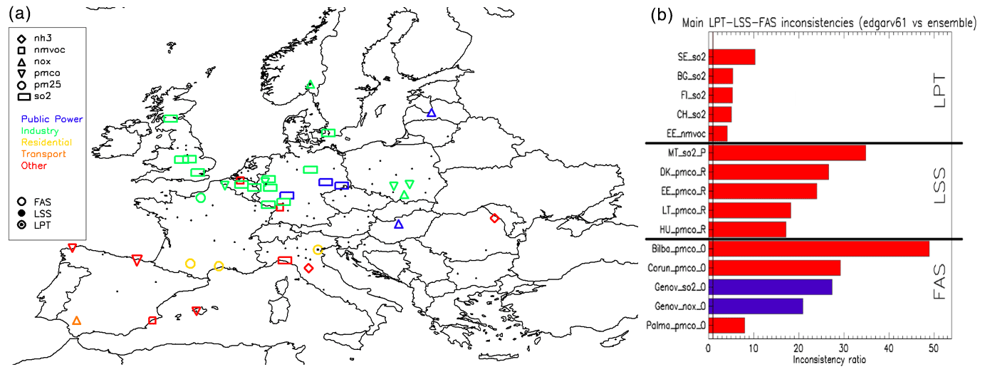
Figure 2 (a) Main inconsistencies spotted at the urban scale for EDGAR when compared to the ensemble. Only the main spatial inconsistency (FAS) for each city is plotted. See the explanation of symbols in the top left of the figure. (b) Major LPT (top five), LSS (middle five) and FAS (lower five) inconsistencies. The first two letters indicate the country code for LSS and LPT, whereas the first four city letters are given for FAS. The red shading indicates an overestimation and the blue shading indicates an underestimation for the EDGAR inventory.

The following main issues can be extracted from Fig. 2 for EDGAR:

• Inconsistencies in SO₂ country totals (LPT) are notably observed in Sweden (factor of 10), Bulgaria, Finland and Switzerland (factor of 5). In the case of Sweden and Finland, we could identify that the main difference comes from the industry sector, particularly the pulp, paper and print sub-sector, for which the inclusion of black liquor use for energy purposes in EDGAR needs to be revised. For Bulgaria, the SO₂ total is dominated by the public power sector for which the activity data, sourced from IEA energy balances, subject to regular updates, influence the magnitude of the differences. According to the Bulgarian Informative Inventory Report (IIR) of emissions in 2022 (IIR, 2022), SO₂ emissions are regularly updated with measurements, which is not the case for the EDGAR emissions estimates; this explains part of the differences. Work is in progress to update SO₂ abatement measures in EDGAR. Another issue that can explain these inconsistencies relates to the different emission factors applied for SO₂ that are based on the sulfur content of fuels, which are not usually reported regularly by countries and are values which are integral to CAMS-REG and EMEP². As a follow-up to this analysis, the SO₂ emission factors for the power sector in EDGAR have been revised taking into account the limits established by the implementation of the Large Combustion Plant Directive (2001/80/EC).

• A large-scale sectorial share (LSS) is found at the country level for SO₂ in Malta for public power (factor of 30) and for residential PMco emissions in Denmark and Estonia (above a factor of 20) and Lithuania and Hungary (about a factor of 10). The large differences in the residential sector are related to biomass burning emissions, both in terms of technology allocation and emission factors applied. Given the large differences with the ensemble, the review of the EDGAR methodology led to the indication that EDGAR estimates needed to be updated, especially in terms of technology allocation. This adjustment is important in order to accurately reflect the current technological structure within that sector. Although the filter on low emission values (relevance test) is applied, it is not effective in the case of Malta because it is a small country where national totals are composed of only a few power plants. The LSS ratios obtained there are not significant as the values estimated for the power plant sector appear to be very small.

• A few large inconsistencies also appear at the local scale (FAS) due to the use of different proxies to spatially distribute emissions. The largest inconsistencies occur for the other sector (likely originating from the waste treatment installations). This can probably be explained by the approach followed by EDGAR for the waste sector for which all emissions are distributed over a few locations only, using E-PRTR locations for landfilling and incineration and population in case of missing information. This results in large differences with other inventories due to the proportion of the emissions being placed within the city area (see Fig. S7 and Sect. S3). A similar issue appears in many north-west EU cities for SO₂ for public power (green rectangles, Fig. 2 left). Work is in progress to update the spatial allocation of the public power and waste sector emissions (Monica Crippa, personal communication, 2023).

The ensemble-based comparison highlights an important number of inconsistencies at the country level. It is important to note that two ensemble members (EMEP and CAMS-REG) use officially reported emissions and therefore rely on similar total emissions per country. On the other hand, EDGAR estimates emissions in an independent bottom-up approach, starting from activity levels and emission factors from international agencies and bodies (Crippa et al., 2018; Oreggioni et al., 2022). This difference in approach can explain a large number of inconsistencies identified for EDGAR, but some of them are very large, especially for SO₂ and PM in the industrial sector. For this particular sector, estimates mostly come from the LPS and E-PRTR databases in EMEP/CAMS-REG, with emissions being mostly based on measurements or facility-level estimates. Such information is not used in EDGAR, where estimates are based on fuel consumption and emission factors that are very general and not plant specific.

4 Application to local inventories: a case study over Poland

4.1 The high-resolution Poland emission inventory

The ensemble-based screening methodology also serves as a benchmark to compare local inventories. In this section, it is applied to the inventory for Poland.

The Central Emission Database (CED) is a local emission inventory designed for Polish national air quality modelling. The CED is based on source location and provides accurate resolution-free data, which can be gridded depending on the requested target resolution for different computational grid configurations over Poland (typically 2.5 km over the entire country and 0.5 km for agglomeration zones). The majority of data are processed with respect to their exact geographical location. Priority is given to the most critical sectors, like residential combustion (described in detail in Gawuc et al., 2021) and road transport. The road transport data presented in this paper (relative to 2019) were based on a traffic model for the major roads in the country. Emissions on minor roads were distributed using the residue values taken from subtracting emissions on major roads from the national totals. The current methodology is based on a smartphone car navigation app, which provides GPS data on road traffic and annual average car speed.

One of the essential components of the CED is the national database on greenhouse gases and other substances emission (called the national database, NB). The NB consists of information on installation and source locations responsible for emissions into the atmosphere. The NB has similarities to the E-PRTR, but, unlike it, it covers all emission sources regardless of type, power or production level. Registered NB users provide information on emission volumes resulting directly from the exploitation of their installations, as well as ancillary processes, which may cause fugitive emissions. To be applied for the CED and air quality modelling, the reported data are categorised into SNAP (Selected Nomenclature for Air Pollution) and converted to the GNFR if needed (Table S1).

The NB is a basis for the GNFR A (public power), B (industry), D (fugitive), E (solvents) and J (waste) emission estimations contributing to the CED. Two approaches are applied to evaluating the CED data. Firstly, as part of each modelling stream (i.e. operational air quality forecast, annual air quality assessment and station representativeness analysis), a comprehensive evaluation is undertaken (a station-by-station time series for over 100 monitoring sites for each pollutant). Moreover, spatial patterns of the increments calculated in the assimilation procedure led to the identity and improvement of the assumptions behind the CED. The database is updated every year, and there is a continuous attempt to improve emission estimates both for the total load and spatial distribution of sources. Modelling results helped to identify missing sources (e.g. resuspension, underestimated agriculture sector and domestic water heating). All sectors in the CED are constantly improved using the best available activity data.

Note that the CED reference year (2019) differs from the ensemble year (2018). Inconsistencies are, however, generally large enough to justify explanations other than those originating from the difference in terms of reference year.

4.2 Comparison of the CED inventory with the ensemble

The ensemble-based screening applied to Poland is performed for 14 cities (see city locations in Fig. 5), five sectors and six pollutants, leading to 420 emission ratios being tested.

Before proceeding with the screening of the local data, we first analyse the level of consistency among the EU-wide inventory over Poland (Fig. 3 is a zoomed-in view of Fig. 1 over Poland). Among the 420 available data, 84 remain after the relevance test (γ_t>0.5). These 84 p–s points serve as a basis to identify inconsistencies (β_t>2). Inconsistencies occur for about 13 % of the relevant p–s points, with a maximum inconsistency (ECI) 2.5 times larger than the assumed level of uncertainty. As seen from the overview table, most of the issues are related to the EDGAR (20) and EMEP (6) inventories, in particular to the residential sector for EDGAR, to the industry sector for CAMS-REG and to the other sector for EMEP. Additional details are provided in Sect. S2.

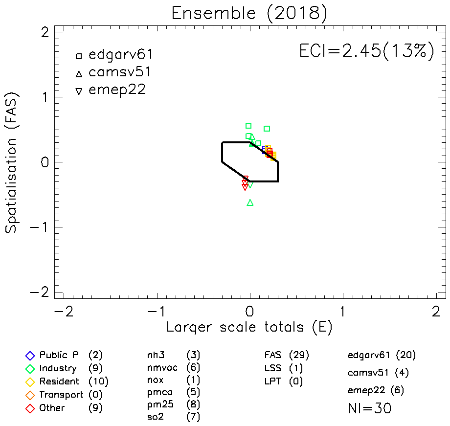
Figure 3 Overview diamonds. The diagram shows the comparison of the three ensemble members (CAMS-REG, EDGAR and EMEP) with the ensemble inventory over Poland. Symbols and colours are as specified in the legend. In all diagrams, only inconsistencies are displayed.

The overview diamond diagram (Fig. 4, left) shows the comparison of the CED local inventory with the ensemble. It indicates that out of the 420 emission ratios being tested, only 73 are associated with relevant emissions, among which 49 (i.e. 67 %) are identified as inconsistencies. The emission consistency indicator (ECI) is around 14, indicating that the maximum inconsistency is larger than the assumed level of uncertainty by a factor of 14. The summary table (at the bottom of Fig. 4) points to the residential and other sectors as having the main issues with NMVOC and PM_2.5 in terms of pollutants. Most inconsistencies originate at the country level and are mostly related to the country sectorial share.

PM residential emissions are systematically larger in the CED than in the ensemble for PM_2.5, whereas they are smaller for PM_co. This can be partially explained by the inclusion of condensable emissions in the CED (not included in EU-wide ensemble). Note that including or not including condensable emissions leads to doubling the total PM_2.5 emissions over Poland due to the importance of residential wood combustion. Also note that in this case, the CED inventory likely performs better than the ensemble, highlighting the fact that ensemble estimates are not necessarily more accurate. Despite this, inconsistencies are flagged and paths for improvements are identified.

Relatively less important, but yet about a factor between 2 and 5, low values occur for SO₂ emissions from the power-generation sector (blue rectangles, Fig. 4). As none of the three EU-wide inventories show an inconsistency for this sector and pollutant, this indicates a general issue between local and EU-wide inventories. This might be explained by the fact that the CED is solely based on the NB, supplied directly with users' data, while EU-wide inventories (EMEP) likely include additional emissions as they are based on overall fuel sales. In addition, point source emissions from the E-PRTR may be different from point source emissions used in national inventories.

The transport and industry sectors show the lowest number of inconsistencies, which is observed by a few points related to those sectors in the diagram (Fig. 4, left). While this is expected for transport which is a diffuse source, this is surprising for the industry as this sector was the main source of inconsistencies at the EU-wide level (see Fig. 3).

Figure 4 (a) Diamond comparison of the local Polish vs. ensemble inventory and (b) comparison of the ensemble top-down members vs. the ensemble restricted to the Polish territory.

Figure 4 (right) highlights the priorities for the analysis. At the country scale, the largest inconsistency occurs for the industrial share of PM_2.5 (a factor of 6 larger in the Polish inventory; LSS; Fig. 4), for PMco and NMVOC from the residential sector by a factor of 5 lower and a factor of 3 larger in the Polish inventory, respectively, as well as for PMco from the other sector (a factor of 3 lower in the Polish inventory). In the case of PM_2.5, the difference can be explained by the fact that the reports provided to the NB are based on user-specific permits, which specify the list of pollutants to be reported, whereas in EU-wide inventories, emissions are generally calculated using official EMEP/EEA emission factors. A comparison of EMEP and CED country totals per pollutant and GNFR sector is available in Table S2.

At the local scale (Fig. 5), the spatial allocation of NMVOC emissions for the other sector leads to important differences in cities like Katowice (a factor of 8; Fig. 4, right), Czestochowa and Krakow. A similar situation is found for PM in Kielce. We see from Fig. 4 that this issue occurs for many cities in the southern part of Poland. The large differences spotted in some cities (e.g. Kielce) are likely caused by emissions from heaps and excavations. While emissions from these sources are accounted for in the CED, only emissions from brown coal excavations (part of the NFR 1B1a) are included in the EMEP inventory. Hence, including all emissions from heaps and excavations in EU-wide inventories would be advisable.

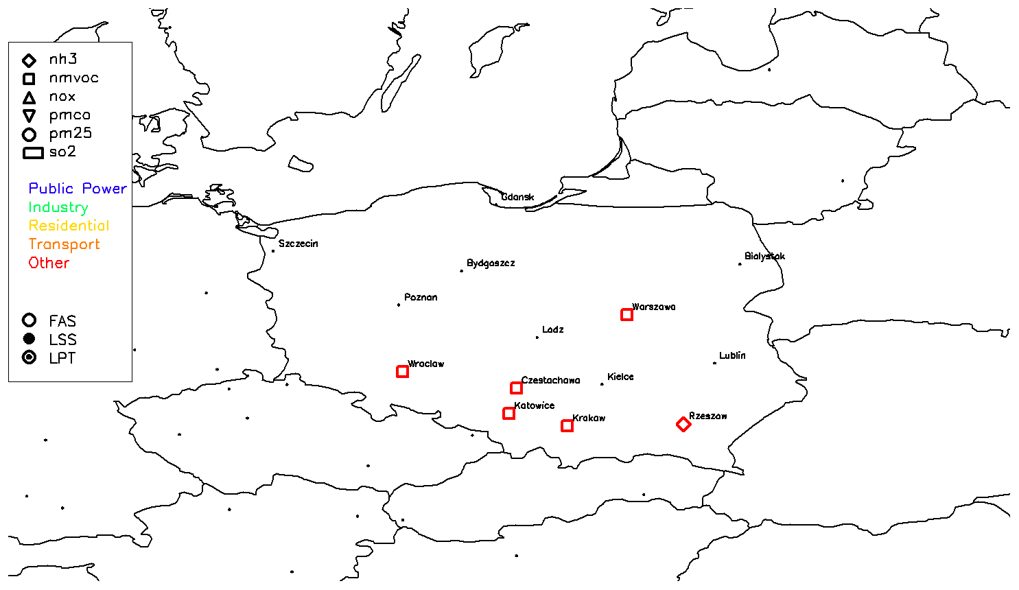
Figure 5 Overview of the inconsistencies for the comparison between local emission inventory in Poland and the EU-wide emission inventory ensemble.

In conclusion, the comparison of the Polish inventory with the ensemble mostly spots issues that are related to a difference in terms of the sectorial share at the country level, explained by the accounting of different sources in the two types of inventories. A similar argumentation can explain part of the large discrepancies observed in some cities. Most of the issues occur for the residential and other sectors and mostly for PM and NMVOC. Although the number of inconsistencies may seem large, many of these are similar for all cities.

Inconsistencies in the spatial distribution of the emissions are relatively minor. This is due to the fact that the EMEP reports for Poland, used in two out of three EU-wide inventories in the ensemble, are gridded by Polish experts, utilising spatial proxies based on the CED activity data for several sectors like stationary combustion, road transport and livestock (last updated in 2021; Bebkiewicz et al., 2022).

5 Added value and limitations of the ensemble approach

EU-wide inventories are not totally independent of each other. The interlinkage between CAMS-REG, EDGAR and EMEP inventories exists. For example, the link between EMEP and CAMS-REG is that both inventories rely on country-reported data and may use the same spatial proxies when the country does not report. EMEP is also linked to EDGAR as it uses, in some cases, EDGAR distribution as a proxy for gridding in case a country is not reporting (CEIP, 2022). Consequently, this interlinkage hides some of the inconsistencies when all inventories behave similarly. It is, however, expected that repeated screenings lead to improvements and to a progressive convergence among inventories, hence reducing the number of flagged inconsistencies.

In our work, the number of members of the ensemble is limited to three. This would be an issue if the goal were to obtain more accurate and robust results with the ensemble. In such a case, the more members, the more robust the results of the ensemble. Our goal is, however, different and consists of creating a benchmark for comparison. Rather than looking at absolute values, we assess differences (between an inventory and the ensemble) for which the accuracy and robustness of the absolute values are of secondary importance.

As emission inventories are characterised by different grid resolutions and sector aggregations, harmonisation is required prior to the screening process for a meaningful comparison. Conversion to a common grid resolution might result in point sources shifting by one grid cell and being in the urban area in one inventory and not in another, although they have the same geographical coordinates in both inventories. However, city-specific diamond diagrams can be used to check if this issue occurs.

While it is more effective for inventory teams to meet and compare approaches in detail to understand and correct differences between inventories, this can be challenging at times, especially in the absence of a specific project to support the work. It must, however, be noted that in many instances, the reporting of an inconsistency, especially when it is very large, leads to a generally straightforward identification of the underlying cause without requiring information that is too detailed regarding the inventories.

The settings used in this work, e.g. the choice of 150 urban areas or the way sectors are aggregated, are arbitrarily fixed. The method allows for flexible choices and could be applied to areas other than urban areas (e.g. complex industrial areas or intensive agriculture land) to assess the consistency with respect to other types of emissions. In terms of sectors, a further disaggregation of the other sector will be performed in the future to better understand where inconsistencies originate from.

6 Conclusions

The approach presented in this work supports the screening and flagging of inconsistencies among inventories through the construction of an ensemble benchmark. This ensemble is created not only to monitor the status and progress made with the development of EU-wide inventories but also to facilitate the comparison among inventories in a relatively simple manner.

The analysis of the EU-wide ensemble and the comparison with its individual members highlighted a large number of inconsistencies. While two out of the three inventories constituting the ensemble behave more closely to each other (CAMS-REG and EMEP), they show inconsistencies in terms of the spatial distribution of emissions. The origin of some differences between these inventories and EDGAR can be identified, but their magnitude remains to be explained. These differences mostly occur for SO₂, PM and NMVOC, for the industrial and residential sectors, and reach a factor of 10 in some instances. The results of the screening provided useful information that allowed identifying necessary improvements of the estimation of air pollutant emissions, in particular for EDGAR, with the PM emissions from the small-scale combustion sector and SO₂ from the industry and power plant sectors. Spatial inconsistencies mostly occur for the industry and other sectors. The fact that the largest inconsistencies are found for sectors where point sources play a major role was expected. Indeed, while a diffuse sector like transport may be distributed quite differently, outliers would not appear as strongly as for point sources.

The application of the ensemble-screening approach to the local inventory for Poland leads to identifying other types of inconsistencies. While we would intuitively expect differences between local and EU-wide inventories to be driven mainly by the spatial distribution of the emissions, this is not always the case in our analysis. Inconsistencies indeed relate mostly to differences in country sectorial shares that result from different sectors/activities being accounted for in the two types of inventories. This can be explained by the fact that some emission sources are omitted in the local inventory due to a lack of appropriate geographically allocated activity data. We identified sectors and pollutants for which discussions between local and EU-wide emission compilers would be needed in order to reduce the magnitude of the observed differences (e.g. in the residential and industrial sectors mostly for NMVOC, PM_2.5 and PM₁₀).

It is also interesting to note that the comparison at the local and EU-wide scale leads to different types of inconsistencies. While the comparison with one local inventory is presented in this work as an example, these comparisons can be systematised to improve the quality of the ensemble.

The ensemble is not meant to be a static entity. It will evolve as inconsistencies are progressively discussed and solved and emission inventories are improved. The ensemble is therefore associated with reference inventory versions as well as with a reference year. In this sense, the ensemble represents a useful tool to motivate the community around a single common benchmark and monitor progress towards the improvement of regional and locally developed emission inventories. It also ensures that improvements become permanent, as forgotten improvements would indeed be flagged again by the system.

Appendix A: List of abbreviations

CAMS-REG	Copernicus Atmosphere Monitoring Services-regional
CED	Central Emission Database
CEIP	Centre on Emission Inventories and Projections
CLRTAP	Convention on Long-Range Transboundary Air Pollution
CO	carbon oxides
ECI	emission consistency indicator
EEA	European Environment Agency
E-PRTR	European Pollutant Release and Transfer Register
EU	European Union
FAS	focus area share
FUAs	functional urban areas
GHGs	greenhouse gases
GNFR	Gridded Nomenclature for Reporting
GPS	Global Positioning System
IIR	Informative Inventory Report
IPCC-AR6	Intergovernmental Panel on Climate Change-Sixth Assessment Report
LPT	large-scale pollutant total
LSS	large-scale sectorial share
NMVOC	non-methane volatile organic carbon
NFR	Nomenclature for Reporting
NH3	ammonia
NOx	nitrogen oxides
OECD	Organisation for Economic Co-operation and Development
NB	national database
PM	particulate matter
PM2.5	particulate matter with a diameter less than 2.5 µm
PM10	particulate matter with a diameter less than 10 µm
PMcoarse	particulate matter with a diameter between 2.5 and 10 µm
SNAP	Selected Nomenclature for Air Pollution
SOx	sulfur oxides
TNO	Netherlands Organisation for Applied Scientific Research
UNECE	United Nations Economic Commission for Europe
UNEP	United Nations Environment Programme