the Creative Commons Attribution 4.0 License.
the Creative Commons Attribution 4.0 License.
 | 03 May 2024
Validation and analysis of the Polair3D v1.11 chemical transport model over Quebec
Shoma Yamanouchi
Shayamilla Mahagammulla Gamage
Sara Torbatian
Jad Zalzal
Laura Minet
Audrey Smargiassi
Ying Liu
Ling Liu
Forood Azargoshasbi
Jinwoong Kim
Youngseob Kim
Daniel Yazgi
Marianne Hatzopoulou
Air pollution is a major health hazard, and while air quality overall has been improving in industrialized nations, pollution is still a major economic and public health issue, with some species, such as ozone (O3), still exceeding the standards set by governing agencies. Chemical transport models (CTMs) are valuable tools that aid in our understanding of the risks of air pollution both at local and regional scales. In this study, the Polair3D v1.11 CTM of the Polyphemus air quality modeling platform was set up over Quebec, Canada, to assess the model's capability in predicting key air pollutant species over the region, at seasonal temporal scales and at regional spatial scales. The simulation by the model included three nested domains, at horizontal resolutions of 9 km by 9 km and 3 km by 3 km, as well as two 1 km by 1 km domains covering the cities of Montréal and Québec. We find that the model captures the spatial variability and seasonal effects and, to a lesser extent, the hour-by-hour or day-to-day temporal variability for a fixed location. The model at both the 3 km and the 1 km resolution struggled to capture high-frequency temporal variability and showed large variabilities in correlation and bias from site to site. When comparing the biases and correlation at a site-wide scale, the 3 km domain showed slightly higher correlation for carbon monoxide (CO), nitrogen dioxide (NO2), and nitric oxide (NO), while ozone (O3), sulfur dioxide (SO2), and PM2.5 showed slight increases in correlation at the 1 km domain. The performance of the Polair3D model was in line with other models over Canada and comparable to Polair3D's performance over Europe.
- Article
(15846 KB) - Full-text XML
- BibTeX
- EndNote


Air pollution is a major health hazard that affects millions of lives globally and is seen as one of the largest contributors to global disability-adjusted life years (GBD 2015 Risk Factors Collaborators, 2016). While air quality overall has been improving in Canada, some species, such as ozone (O3), still regularly exceed the standards set by governing agencies (e.g., Ministry of the Environment and Climate Change, 2016). Furthermore, the Canadian government (Health Canada, 2022a) estimated in 2019 that the economic impacts of air-quality-related health risks are over CAD 100 billion per year and that air pollution is linked to 15 300 premature deaths every year in Canada.
Industrial and traffic emissions play a large role in determining urban air quality (e.g., Rai, 2016; Batisse et al., 2017; Wallington et al., 2022; Health Canada, 2022b). In the province of Quebec in Eastern Canada, 410 premature deaths were attributed to traffic-related air pollution in 2015 (Health Canada, 2022b). Quebec sees higher levels of particulate matter than the national average and similar results for nitrogen dioxide (NO2) and sulfur dioxide (SO2). Additionally, industrial emissions and proximity to industrial facilities in Quebec have been associated with adverse health outcomes such as asthma onset in childhood (Buteau et al., 2020), short-term risk of hospitalization in children (Brand et al., 2016) and a decrease in lung function (Smargiassi et al., 2014). As opposed to traffic emissions which mainly take place in densely populated areas, high-emitting industries in Canada are also found in rural areas (Jeong et al., 2011). These regions typically do not have other major sources of air pollution, which results in large gradients in pollution levels in nearby communities.
Environment and Climate Change Canada (ECCC) operates about 250 air pollutant monitoring stations as part of their National Air Pollution Surveillance (NAPS) program (NAPS, 2016), of which 131 are in Quebec (and some may only be reporting limited time periods and/or limited pollutant species). Given the size of the country and the province, this is far too sparse to be useful in conducting spatial variability analyses of air pollutants. Modeling the sources, chemistry, dynamic transport of atmospheric pollutants is crucial in understanding tropospheric pollution events and mitigating health impacts by identifying affected regions and sensitivity to various emissions. There are mainly two chemical transport models (CTMs) used in Canada, GEM-MACH run by ECCC and the US EPA's Community Multiscale Air Quality Modeling System (CMAQ). While the ECCC GEM-MACH has been used to model the atmosphere over Canada including Quebec (Chen et al., 2020; Health Canada, 2022b), we attempt to assess the performance of and validate the Polair3D CTM of the Polyphemus air quality modeling platform (Mallet et al., 2007) coupled with emissions derived from both ECCC and the United States emission inventories using the Sparse Matrix Operator Kernel Emissions (SMOKE) emissions-processing system, for key pollutant species: carbon monoxide (CO), O3, NO2, NO, SO2, and particulate matter smaller than 2.5 µm in diameter (PM2.5). The Polair3D model has seen little use over North America and particularly over Canada, aside from one example over Ontario, Canada (Minet et al., 2021), and a coarse-resolution study covering all of North America by Sartelet et al. (2012). Unlike CMAQ, which is mainly used at larger, regional scales at coarser resolutions (i.e., horizontal resolutions higher than ∼1 km2), Polair3D is known to be robust at these higher resolutions (Thouron et al., 2017), and we aim to assess the model performance at these higher resolutions as well as at coarser resolutions with larger modeling domains. In this study, we aim to present a novel use of this model over Quebec, Canada, using a longer modeling period and a larger modeling domain, to assess the ground (surface) level model performance at seasonal temporal scales and at regional spatial scales.
2.1 Model setup
The Polyphemus platform (Mallet et al., 2007) was used for this analysis. Polyphemus is an open-source suite of models developed at the Centre d'Enseignement et de Recherche en Environnement Atmosphérique (CEREA), and in this study, Polair3D (Sartelet et al., 2002; Mallet and Sportisse, 2004; Pourchet et al., 2005; Boutahar et al., 2004), a CTM within the Polyphemus platform, was utilized. The newest version (v1.11) of the model (Kim et al., 2023) was used, with an updated aerosol chemistry module called SSH-aerosol (Sartelet et al., 2020). This module combines SCRAM (Size-Composition Resolved Aerosol Model), which simulates the dynamics and the mixing state of atmospheric particles; SOAP (Secondary Organic Aerosol Processor), which models the partitioning of organic compounds; and H2O (hydrophilic/hydrophobic organics), which simulates the formation of semi-volatile organic compounds formed via the oxidation of volatile organic compounds (VOCs). Polair3D is a Eulerian atmospheric CTM and includes preprocessing modules for formatting and creating binary input files for meteorology, biogenic emissions, surface deposition, and initial/boundary conditions. Anthropogenic emissions inventories are discussed in Sect. 2.2. For calculating biogenic emissions and deposition at the surface, land-use data from GLC2000 were used (Bartholomé and Belward, 2005).
The meteorology field was taken from pre-run WRF data (NCAR, 2023). The modeling domain comprises four domains that have 27, 9, 3, and 1 km grid spacing, respectively, with two-way nesting. The number of vertical levels is 42, spanning from the surface to 100 hPa. Initial and lateral boundary conditions of meteorology were provided by the North American Regional Reanalysis (NARR) (Mesinger et al., 2006), which is available at a 32 km grid spacing with 30 vertical levels. Each 30 h forecast was initialized every 00:00 UTC and had a 6 h spin-up time. Thus, the first 6 h of forecasts are discarded and replaced with forecasts initiated with the previous cycle for overlapping times. Grid nudging was applied for horizontal wind, temperature, and humidity for vertical levels above the planetary boundary layer (PBL) height in the largest domain. Parameterization schemes used in the simulation are as follows: the Purdue Lin scheme (Chen and Sun, 2002) for microphysics, Rapid Radiative Transfer Model for GCMs (RRTMG) shortwave and longwave schemes (Iacono et al., 2008), Mellor–Yamada–Janjic PBL scheme (Janjić, 1994), Grell–Devenyi ensemble scheme (Grell and Dévényi, 2002) for cumulus parameterization which was applied only to domain 1 and 2, Unified Noah land surface model (Chen and Dudhia, 2001), and a three-category urban canopy model (Chen et al., 2011) for urban areas. WRF temperature, as well as wind speed/direction, was compared against observational data from meteorological stations operated by ECCC prior to using them in Polair3D.
From this WRF configuration, meteorology from the 9, 3, and 1 km domains was used. The model configuration is as follows: the model was run in three nested domains; the largest and coarsest-resolution domain was roughly 9 km by 9 km grid-cell resolution (edges), and within it, a smaller domain of about 3 km by 3 km resolution was run, and lastly, 1 km by 1 km resolution runs were performed over the cities of Montréal and Québec. The modeling domains are shown in Fig. 1 (note that parts of the 9 and 3 km domains include the United States (US)). The model was run for four seasons from 2018, with 4 weeks per season (January for winter, April for spring, July for summer, and October for fall), for a total of 16 weeks of model data. Spin-up was done for 1 week for each run. Boundary conditions for the outermost domain and the initial conditions for each of the runs were derived from CAM-Chem assimilated data (Tilmes et al., 2015).
The model was run with a 10 min time step, and output was averaged and saved hourly. The model was run with vertical grids going up to 6000 m, but only data from the lowermost layer (surface) were saved. The vertical resolution is as follows: 0, 20, 40, 90, 150, 250, 400, 800, 1500, 2400, 3500, and 6000 m. For 1 km resolution runs, the small domain size led to numerical instabilities, and the time steps were lowered to 5 and 1 min for the cities of Montréal and Québec, respectively. In this study, CO, O3, NO2, NO, SO2, and PM2.5 from the model were examined, although data for other species were also saved.
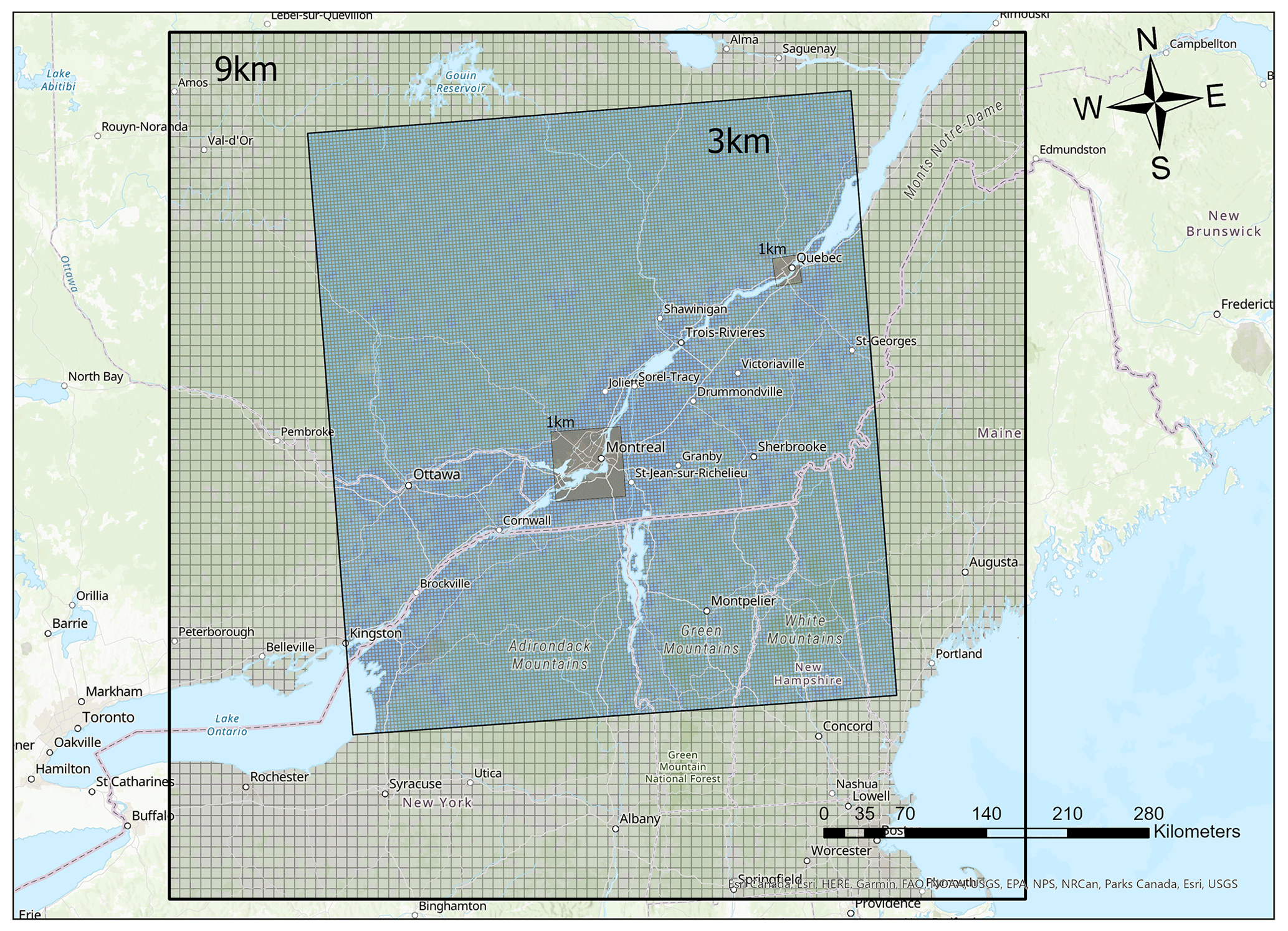
Figure 1The modeling domains used in this study.
2.2 Emissions
A Sparse Matrix Operator Kernel Emissions (SMOKE) emissions-processing system was used to prepare the Polair3D emissions input files (CMAS-SMOKE, 2023). Emission processing involves three major steps: spatial allocation, temporal allocation, and chemical speciation. Canadian and US emissions in the domain were calculated based on SMOKE-ready formats of the Canadian emission inventory (Sassi et al., 2021) and US National Emissions Inventory (EPA: Emissions Modeling Platforms, 2023), along with their temporal allocation and chemical speciation data. Spatial allocations for the three nested domains were generated using both Canadian and US spatial allocator inputs (CMAS-SA, 2023; CMAS-DB, 2023).
Canada's Air Pollutant Emissions Inventory (APEI) also known as the Canadian criteria-air-contaminants (CACs) emissions inventory, is prepared and published by ECCC. The APEI is a comprehensive inventory of anthropogenic emissions of 17 air pollutants including CO, ammonia (NH3), nitrogen oxides (NOx), PM2.5, particulate matter smaller than 10 µm in diameter (PM10), SO2, and VOCs at the national, provincial, and territorial levels. It is compiled from many different data sources. The APEI is developed by the Pollutant Inventories and Reporting Division (PIRD) of ECCC. The inventory databases compiled by PIRD are modified by the Air Quality Modeling Applications Section (AQMAS) of ECCC for emissions processing with SMOKE. For further details of the SMOKE-ready format of the Canadian 2015 APEI inventory, refer to Annex 2 of the 1990–2015 Air Pollutant Emission Inventory Report (Environment and Canada, 2017).
The US National Emissions Inventory (NEI) is the second inventory used in this study. NEI includes emissions for the six criteria air pollutants (CAPs) and 187 hazardous air pollutants. The CAP-related emissions are NH3, CO, Pb, NOx, particulate matter (PM2.5, PM10, organic carbon, and black carbon), SO2, and VOC. Data on US emissions are derived in several ways: continuous measurements, estimates based on infrequent source samples, and estimates based on average emission rates. In this study, we use a combination of SMOKE-ready formats of NEI 2014 and 2017 inventories from EPA (EPA: Emissions Modeling Platforms, 2023).
The emission sectors nonpoint, on road, and nonroad in both Canadian and US inventories were processed in SMOKE as area sources. The point source sectors in both inventories were processed as either two-dimension (2D) or three-dimension (3D) (layered) elevated point source emissions. Emissions from point sources such as airports and mines are considered 2D elevated sources. Industrial emissions (e.g., electric power generation, commercial facilities) are calculated as 3D layered emissions. SMOKE analyzes the stack parameters of each facility as well as the meteorology to determine the layers' emissions. SMOKE accesses the stack parameters such as the height, the diameter, and the temperature directly from the industrial emissions reported in the Canadian and US inventories. Meteorology-Chemistry Interface Processor (MCIP) was used to generate the necessary meteorology files (e.g., GRID_CRO_2D, MET_CRO_2D, MET_DOT_3D) for SMOKE volume emission processing (EPA-CMAQ, 2023). There are known aberrations in the ECCC off-road emissions in January. To correct for this, the off-road emissions in January were replaced by those of April (off-road emissions do not vary significantly by season). These aberrations were not seen in any of the other sectors nor in any of the other months.
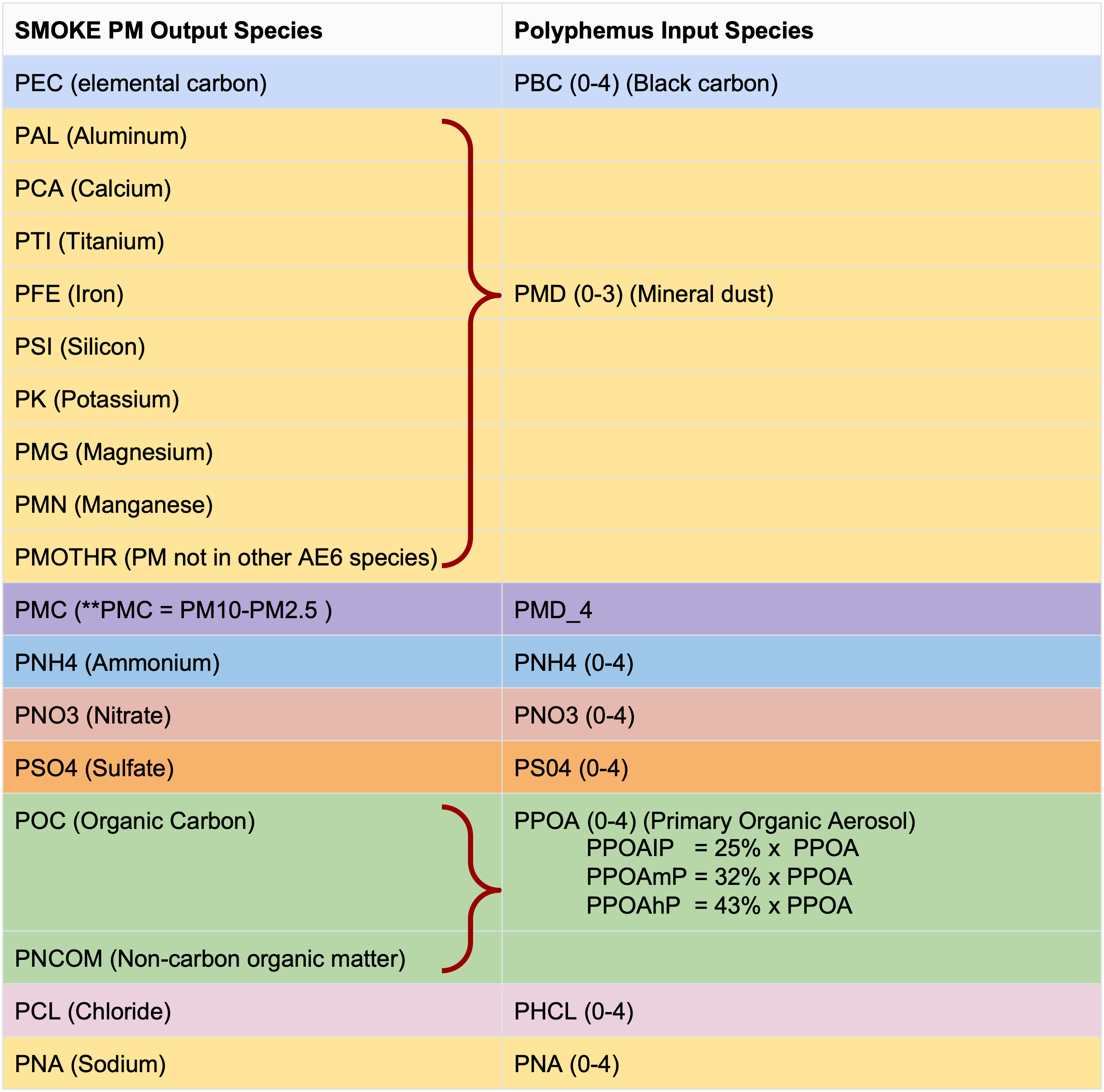
The Polair3D model contains a Size-Composition Resolved Aerosol Model (SCRAM). Thus, the PM AE6 speciated SMOKE output must be incorporated into an input for SCRAM. This conversion is shown in Table 1. The size distribution of the PM species was applied based on the SNAP (Selected Nomenclature for Air Pollution) sectors. The SNAP sectors include combustion in energy and transformation industries; non-industrial combustion plant; combustion in the manufacturing industry; production processes; extraction and distribution of fossil fuels and geothermal energy; solvent and other products; road transport, other mobile sources, and machinery; waste treatment and disposal; and agriculture (EMEP/EEA, 2019). A 5-bin size distribution was applied to each species that was derived from the 10-bin SNAP size distribution values consistent with the Polair3D inputs. For the Polair3D model, primary organic aerosol (POA) species also need to be divided into three categories based on volatility. Hence, first, the POA species were divided into low (POAlP), medium (POAmP), and high (POAhP) volatility, and then we applied the 5-bin size distribution for each subspecies.
2.3 Surface observations
Model results were compared against surface observations to validate the model and assess its performance in modeling key air pollutant species at the surface level. Surface observations collected as part of the National Air Pollution Surveillance (NAPS) program (NAPS, 2016) were used in this analysis.
The air pollution species examined in this study (CO, O3, NO2, NO, SO2, and PM2.5) are reported by some but not all NAPS sites; many NAPS sites only report some of the species, and some sites may not have data during the modeling time period.
To assess the modeling performance, several statistics were examined: Pearson correlation coefficient (R), mean relative difference (MRD), mean squared error (MSE), mean bias (MB), and normalized mean bias (NMB). MRD, MSE, NB, and NMB were calculated by subtracting NAPS from the model (i.e., , , , and ). These statistics were chosen following Emery et al. (2017).
Additionally, for NO2 and PM2.5, the model was compared against assimilated monthly ground level national LUR (land use regression) dataset products from the Canadian Urban Environmental Health Research Consortium (CANUE) (for NO2) (Hystad et al., 2011; Weichenthal et al., 2017; DMTI Spatial Inc., 2015) and Atmospheric Composition Analysis Group (ACAG) for (PM2.5) (van Donkelaar et al., 2021). The CANUE NO2 dataset was developed from 2006 NAPS data using the land use regression model taking into account various geographic variables (road length within 10 km, area of industrial land use within 2 km, and summer rainfall) and satellite data (from 2005 to 2011) (Hystad et al., 2011). In this dataset, monthly averages of NO2 are given for each Canadian postal code (DMTI Spatial Inc., 2015), and the comparison analysis with the model was done using the 3 km resolution model binned into the closest model grid cell. The 2018 monthly dataset was used. The ACAG PM2.5 dataset is derived by assimilating aerosol optical depth (AOD) retrievals from the NASA MODIS, MISR, SeaWiFS, and VIIRS instruments with the GEOS-Chem chemical transport model and was calibrated to global ground-based observations using a geographically weighted regression (van Donkelaar et al., 2021). The dataset has a resolution of 0.01° by 0.01°. The comparison analysis was done using the 3 km model resolution, and the ACAG dataset was binned into the Polair3D similar to the analysis done with the CANUE national LUR dataset. The 2018 monthly dataset was used.
2.4 Test scenarios
As discussed in Sect. 1, industrial emissions have been associated with adverse health outcomes. Understanding the behavior of the model under various emissions scenarios is important for performing pollution exposure analyses. To enrich the model validation findings and to qualitatively assess the behavior of the Polair3D model under varying emissions scenarios, a run with no industrial emissions was performed for the same domain and time frames. Other emissions (such as biogenic and traffic emissions) were kept the same. All other variables and input files, including the meteorology and the model configurations, were kept the same as the base case (i.e., with all emissions).
Additionally, two test scenarios, one with only the emissions from smelter, refinery, and foundry industries suppressed and another scenario with only the emissions from paper and pulp industry turned off, were run. These scenarios were adapted from a study by Liu et al. (2024). As with the no-industry scenario, all other variables and input files were kept the same as the base case.
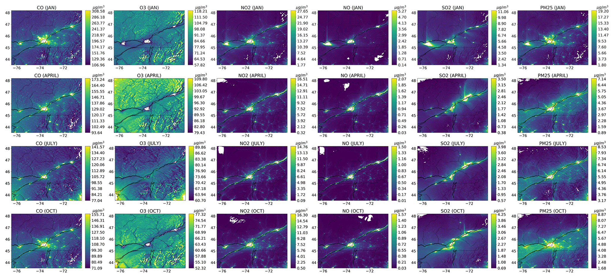
Figure 2Monthly averages (January, April, July, and October, from top to bottom) of the Polair3D model at the 3 km resolution for (from left to right) CO, O3, NO2, NO, SO2, and PM2.5. All units are in µg m−3. Note that if the concentrations are above or below the scale (chosen here to exclude the lowest and the highest percentile), the figures will show white; this was done to preserve important spatial details in the mid-range of the data.
3.1 3 km resolution
The 3 km modeled monthly averages (for January, April, July, and October) for the entire domain are presented in Fig. 2 for CO, O3, NO2, NO, SO2, and PM2.5 (a note about these figures is that if the concentrations are above or below the scale, chosen here to exclude the lowest and the highest percentile, the figures will show white; this was done to preserve important spatial details in the mid-range of the data). For O3, 8 h maximum daily average (MDA8) was examined as recommended by Emery et al. (2017).
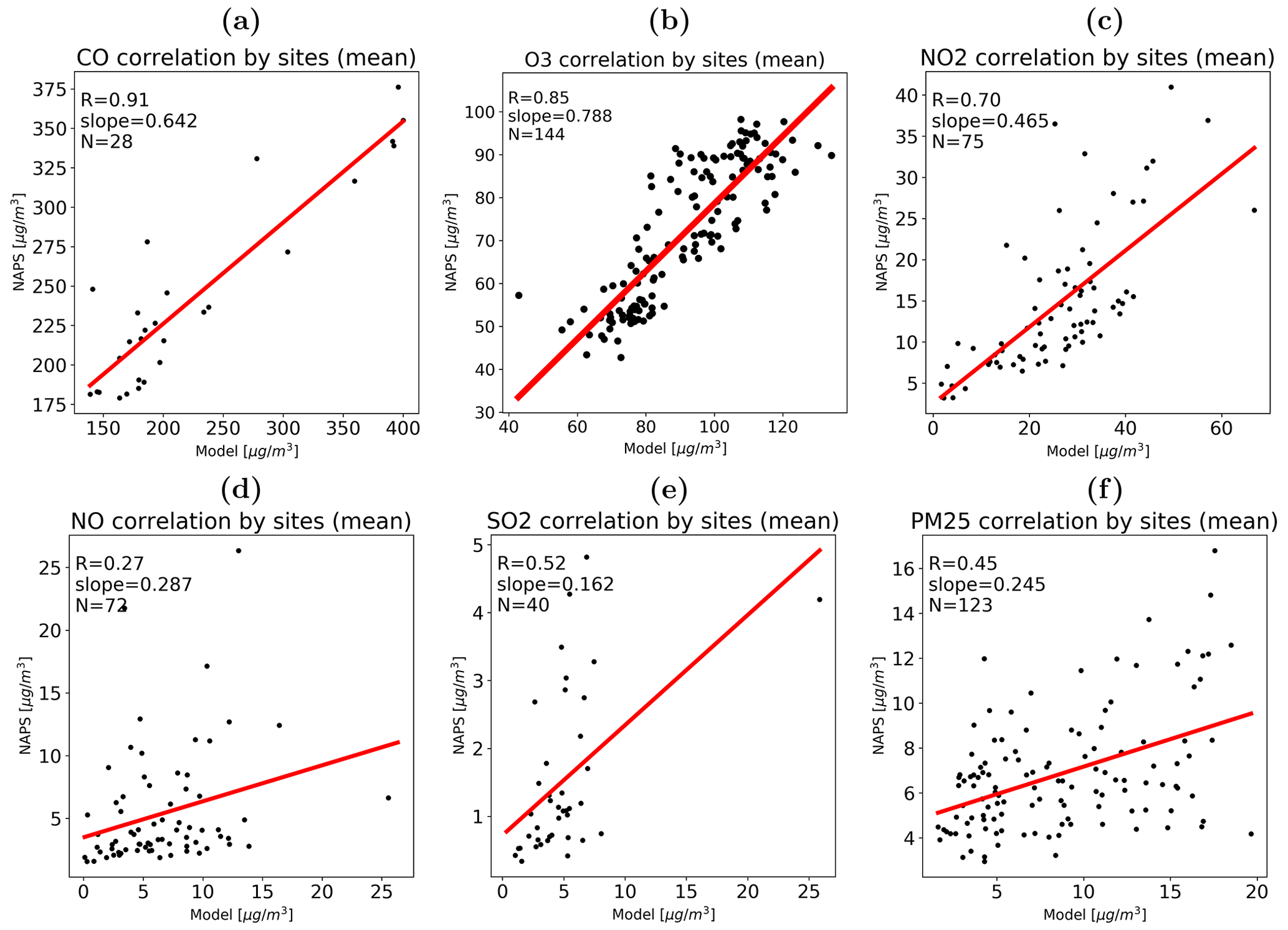
Figure 3Monthly average site-wide correlation plots at the 3 km resolution for CO, O3, NO2, NO, SO2, and PM2.5 for panels (a), (b), (c), (d), (e), and (f), respectively. For O3, MDA8 was first calculated and used for this analysis (see Sect. 3.1 for more detail). All units are in µg m−3.
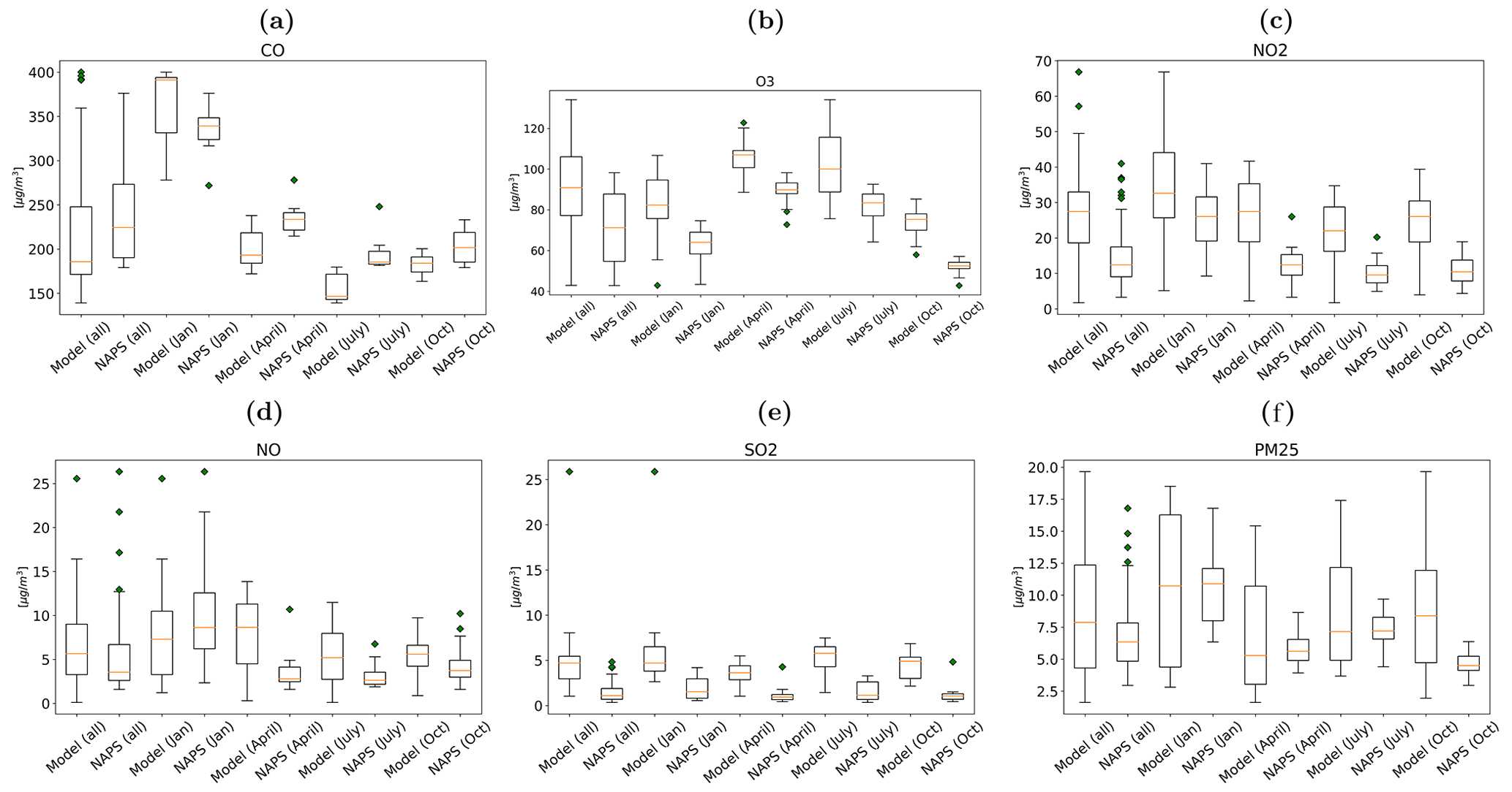
Figure 4Monthly average site-wide comparison box plots at the 3 km resolution for (a) CO, (b) O3, (c) NO2, (d) NO, (e) SO2, and (f) PM2.5. For O3, MDA8 was first calculated and used for this analysis (see Sect. 3.1 for more detail). All units are in µg m−3.
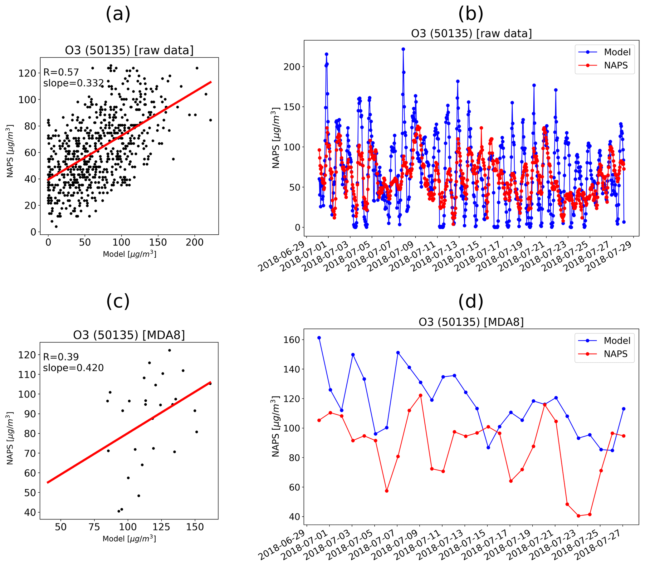
Figure 5Correlation ((a) for raw data and (c) for MDA8) and time series ((b) for raw data and (d) for MDA8) of NAPS data and the modeled O3 over a NAPS site in Montréal (NAPS ID: 50135) in July. All units are in µg m−3.
A site-wide analysis, that is, comparing monthly averages across all NAPS sites, resulted in higher correlation for CO, O3, and NO2 than NO, SO2, and PM2.5. CO exhibited a high correlation coefficient (R) of 0.91 across 28 data points, while NO showed the lowest correlation at R=0.27 (see Table 2). Correlation plots for all species at the 3 km resolution can be found in Fig. 3. Both O3 and NO showed higher correlation in winter than in the summer, going from R=0.83 in January down to 0.63 in July for O3 and from 0.27 to 0.03 for NO. While NO2 correlation did go down over the summer, it was not to this extent (R=0.69 in January, down to 0.53 in July). Sartelet et al. (2012) reported, in their study using the Polair3D model covering all of North America (at a coarser resolution of 0.25° by 0.25°), O3 correlation of 0.604, which is comparable to our overall correlation of 0.85. Both modeled O3 and NO2 showed some overestimation bias, with MRD = 21.4 % and 33.5 %, respectively (see Fig. 4). Indeed, NO2 and SO2 both showed overestimation biases, despite CAC emissions being thought to underestimate emissions of these species (Krzyzanowski, 2009). Minet et al. (2021) saw large overestimations of O3 in their Polair3D validation effort and attributed it to MOZART4 boundary conditions; the boundary conditions in this study were derived from CAM-Chem. Also of note is the result that MRD in O3, a photochemically reactive pollutant that typically peaks in summertime in the troposphere, was similar in both summer and winter (18.2 % and 23.5 % for July and January, respectively).
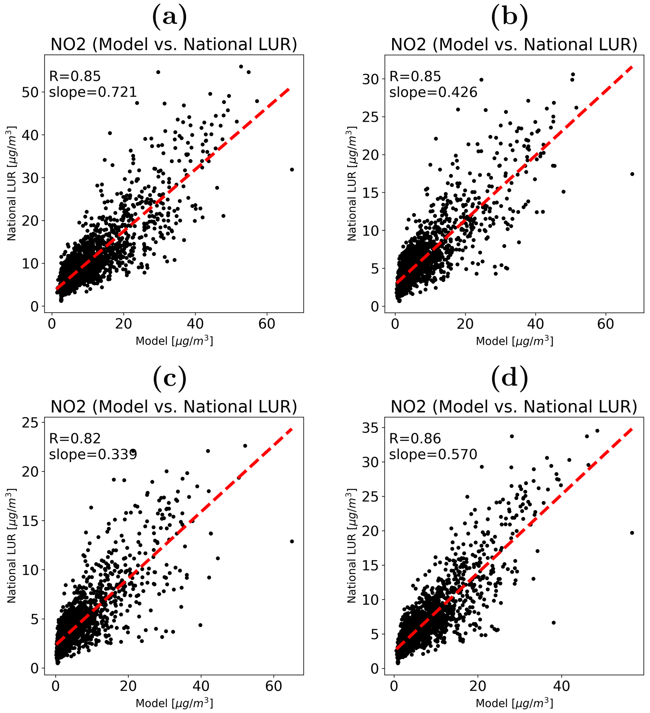
Figure 6Monthly model vs. CANUE national LUR NO2 correlation plots for (a) January, (b) April, (c) July, and (d) October. All units are in µg m−3.
NO, on the other hand, showed overestimation overall (see Fig. 3d), but the calculated MRD was −59.2 % (indicating underestimation), likely resulting from a few very high values seen in the NAPS data. This is similar to the GEM-MACH model over North America, which also overestimated CO, O3, NO2, and NO (Stroud et al., 2020; Makar et al., 2015). In fact, the GEM-MACH model over Toronto, Canada, was shown to overestimate NO2 to a larger extent than O3, much like the results presented here (Stroud et al., 2020).
PM2.5 performance showed mixed results; the bias was relatively small with an overall MRD of −3.9 %, but correlation varied significantly from R=0.82 in January to R=0.36 in July (and 0.45 overall). Minet et al. (2021) also noted the poor correlation for modeled PM2.5 in their study that examined Polair3D performance during a particular summer day (in August). The model performing worse in the summer was a common theme seen in all species except for SO2, which had the opposite trend with R=0.57 in January and 0.66 in July. The correlation is comparable to a study by Sartelet et al. (2012), who reported a correlation of 0.504 for PM2.5. Modeled SO2 showed overestimation as well, with MRD =66.5 %. Another noteworthy point here is that correlations of CO were, in most cases, better than those of other primary (emitted) pollutants like NO2, NO, and SO2; this may be explained by uncertainties in emissions (Kim et al., 2018).
The model performance was more challenging when looking at individual sites. An example of O3 time series and correlation plots from January is shown in Fig. 5; this plot shows the NAPS data and the modeled O3 over a NAPS site in Montréal (NAPS ID: 50135) in July (both the raw comparison and comparison using the MDA8 metric are shown). There was considerable variability in correlation from site to site; this site showed relatively good correlation, especially for the raw comparison. The model showed relatively small biases for O3 and captures the overall ranges seen in observational data (NAPS mean values were within the model mean ± 1 model standard deviation for most sites). MDA8 O3 comparison generally fared better in winter months (January), with worse correlation in other times of the year; the July plot shows worse correlation with the MDA8 than with the raw comparison.
For all species, there was considerable variability in correlation coefficients from site to site, and resampling (e.g., 6 h average) the dataset did not lead to improved correlation (up to 48 h averages were tried in this analysis), although as noted above, for O3, comparison using MDA8 did result in better correlation. NAPS data are reported to the nearest integer values, meaning the data are quite coarse, leading to discretization artifacts that can clearly be seen in Fig. 5a. These results suggest that the model is better at capturing the spatial variability and seasonal effects rather than hour-by-hour or day-to-day temporal variability for a fixed location. Furthermore, NAPS sites are categorized into several site types, including regional background (RB), general population exposure (PE), and transportation influenced (T), and when looking at correlations from this perspective, the highest O3 correlation was seen with the RB sites that indicate that the model is able to capture the overall amount of background O3 that is generated/destroyed. Correlations for NO2 and NO were poor for PE sites (generally in urban areas), suggesting that there are large uncertainties in emissions.
Comparisons with the national LUR monthly NO2 dataset show relatively good agreements for all 4 months. R ranged from 0.82 in July to 0.86 in October. The correlation plots can be seen in Fig. 6. Although the model mean was higher (i.e., the model is overestimating) for all months except for January, MRD ranged from −48 % to −22 %. This indicates that in places where the model is underestimating, the model underestimates by a large margin; because MRD calculation involves dividing by the model value, if the model values are small (and smaller than the national LUR values), the MRD becomes a large negative number. The collation against ACAG PM2.5 showed relatively worse correlations. The highest R was 0.59 in April, and the worse correlation was R=0.45 in October. The correlation plots can be seen in Fig. 7. MRD ranged from −80 % to −10 %, and the model mean was lower than the ACAG mean for all months except for October.
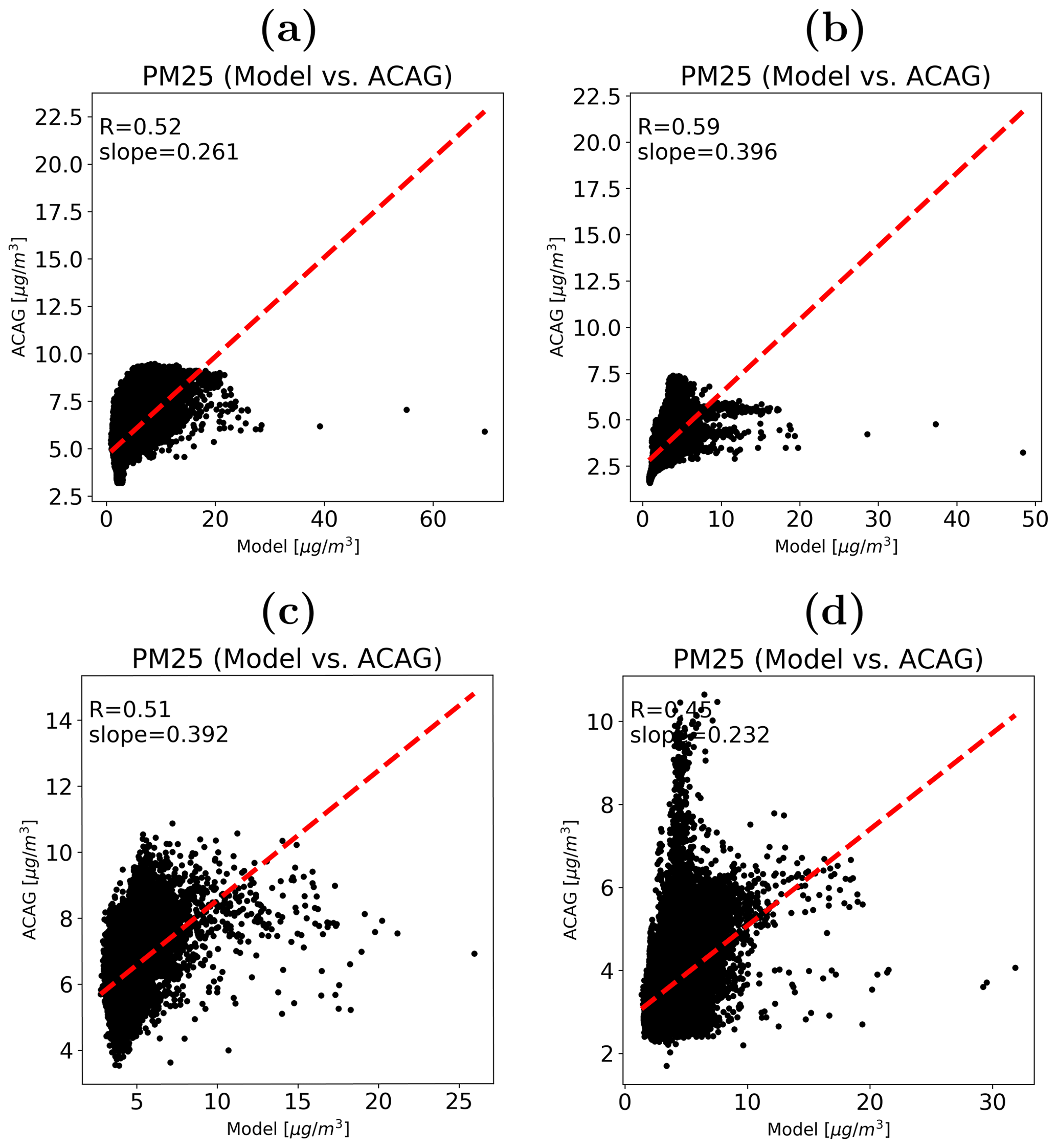
Figure 7Monthly model vs. ACAG PM2.5 correlation plots for (a) January, (b) April, (c) July, and (d) October. All units are in µg m−3.
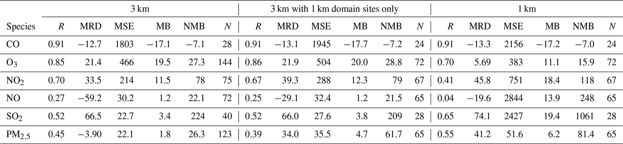
Table 2Site-wide comparison summary table showing correlation (R), mean relative difference (MRD), mean squared error (MSE) (µg m−3), mean bias (MB) (µg m−3), normalized mean bias (NMB) (see Sect. 2.3 for more detail), and number of data points (N), using data from all four simulation months (January, April, July and October) for the 3 km run, 3 km run with comparisons restricted to NAPS monitoring sites found in the 1 km domain only, and 1 km run. For O3, MDA8 was first calculated and used for this analysis (see Sect. 3.1 for more detail).
3.2 1 km resolution
The 1 km model was run over the cities of Montréal and Québec (see Fig. 1 for the domains). As noted in Sect. 2, the time step of the model was shortened to 5 and 1 min for the cities of Montréal and Québec, respectively, down from 10 min, to increase model stability at these small domains (see Sect. 2.1). The modeled monthly averages (for January, April, July, and October) for the entire domains are presented in Figs. 8 and 9 (for the cities of Montréal and Québec, respectively) for CO, O3, NO2, NO, SO2, and PM2.5.
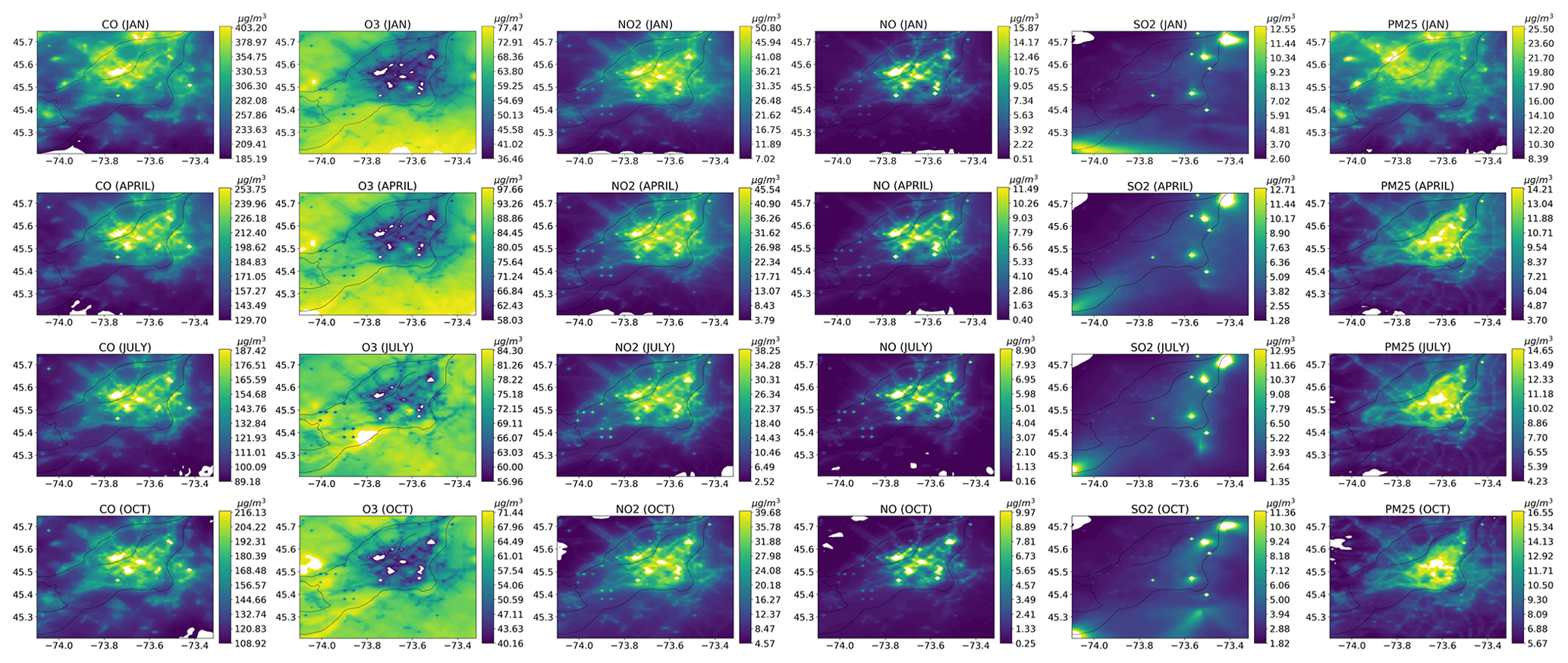
Figure 8Monthly averages (January, April, July, and October, from top to bottom) of the Polair3D model at the 1 km resolution over Montréal for (from left to right) CO, O3, NO2, NO, SO2, and PM2.5. All units are in µg m−3.
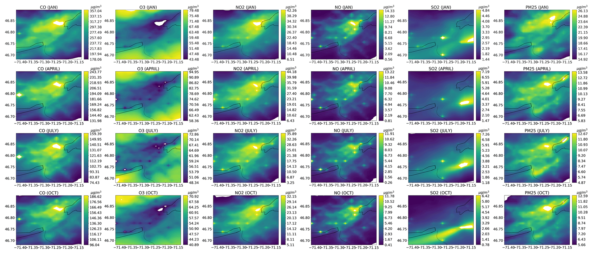
Figure 9Monthly averages (January, April, July, and October, from top to bottom) of the Polair3D model at the 1 km resolution over Québec for (from left to right) CO, O3, NO2, NO, SO2, and PM2.5. All units are in µg m−3.
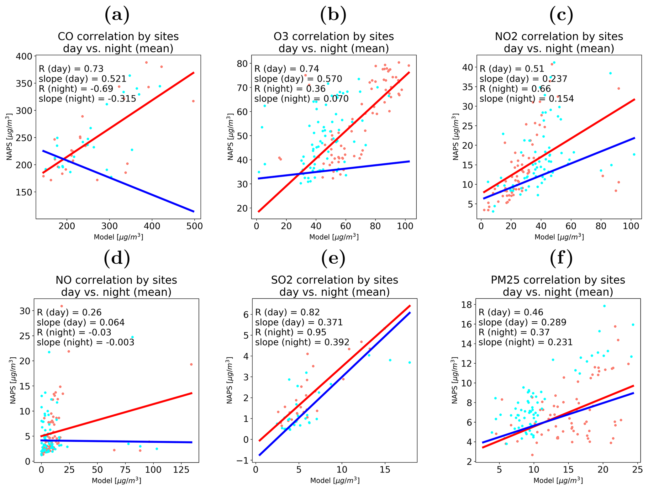
Figure 10Monthly average site-wide correlation plots, separated between day (red) and night (blue) data points, at the 1 km resolution for (a) CO, (b) O3, (c) NO2, (d) NO, (e) SO2, and (f) PM2.5. All units are in µg m−3.
When comparing the biases and correlation at a site-wide scale, the higher-resolution 1 km runs did not result in strictly better performance. Indeed, when analyzing the same sites (i.e., restricting the 3 km analysis to the NAPS sites seen in the smaller 1 km run), the coarser 3 km model showed slightly higher correlation for CO, NO2, and O3, and while SO2 and PM2.5 showed increases in correlation when running at the 1 km resolution, the differences were small, for example, going from 0.52 to 0.65 (for 3 and 1 km, respectively) for SO2 (see Table 2; note that MDA8 metric was used for O3). Examining the model performance site by site showed similar results. Running the model at an increased resolution may be an effective way to downscale the data, but it does not appear to make the simulation more temporally accurate. Similar results were reported by Russell et al. (2019). Their model (GEM-MACH) did not show improvements in standard scoring methodologies (such as correlation with surface observation sites) when increasing their model resolution from 2.5 to 1 km.
To assess the model performance during the daytime versus nighttime, a similar site-wide analysis was done but this time separating the daytime data and nighttime data. The results can be seen in Figs. 10 and 11, for correlation and box plots, respectively. One noteworthy result is that the slope was higher during the day for all species except SO2. Correlation was higher for CO, O3, NO, and PM2.5 and was slightly lower for NO2 and SO2. Furthermore, O3, a secondary pollutant that is created and destroyed photochemically and thus heavily affected by sunlight, showed higher correlation during the day than during the night (see Fig. 10 correlation plot) and at the same time showed large underestimation biases during the night (see Fig. 11 box plot). This suggests that the model is capable of modeling O3 during the day but struggles to simulate the background O3 during the night when photochemical reactions are low and/or nonexistent. For CO, correlation was significantly higher during the day than during the night (R=0.73 versus −0.69), although the difference was less extreme when looking at individual months.
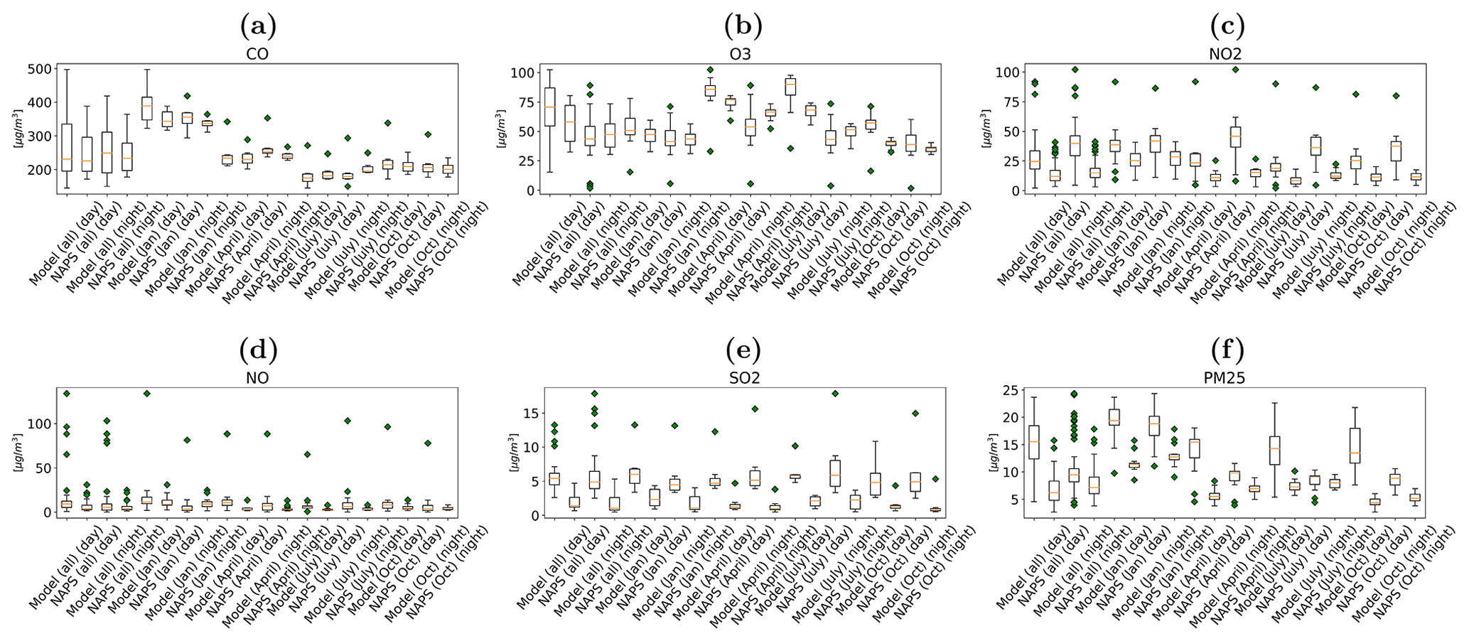
Figure 11Monthly average site-wide box plots, separated between day and night data points, at the 1 km resolution for (a) CO, (b) O3, (c) NO2, (d) NO, (e) SO2, and (f) PM2.5. All units are in µg m−3.
3.3 Comparison with other models
Polair3D performance over Canada is in line with models, such as GEM-MACH, over Canada. A study by Russell et al. (2019) which examined the performance of GEM-MACH over Alberta, Canada, at both 1 and 2.5 km resolutions saw similar correlations. In their study, they calculated correlation coefficients for O3, SO2, and PM2.5 to be 0.496 (0.506 for 1 km), 0.290 (0.230 for 1 km), and 0.201 (0.216 for 1 km), respectively, compared to 0.85 (0.70 for 1 km), 0.52 (0.65 for 1 km), and 0.45 (0.55 for 1 km) for our study (see Table 2). Russell et al. (2019) found normalized mean biases for O3, SO2, and PM2.5 to be 52.7 % (55.9 % for 1 km), 113 % (137.6 % for 1 km), and −26.8 % (−25.6 % for 1 km), respectively, compared to our NMB of 27.3 % (15.9 % for 1 km), 224 % (1061 % for 1 km), and 26.3 % (81.4 % for 1 km).
Comparing against a similar study by Stroud et al. (2020) that examined short-term GEM-MACH performance over Toronto, Ontario, Canada, for O3 and NO2 at both 10 and 2.5 km resolution using NAPS surface observations also shows comparable correlations. While their modeling duration was much shorter (limited to several days in July 2015) and thus a direct comparison could not be made, their study saw correlation coefficients of 0.62 and 0.77 for O3 and NO2, respectively, compared to 0.85 and 0.70 for our 3 km resolution runs. Similar to the comparison with Russell et al. (2019), our model showed higher biases; they saw O3 normalized mean biases of 5.4 % with their 2.5 km resolution run compared to 21.4 % for our 3 km run and 28.2 % for NO2 compared to 78 % for our 3 km run.
Our Polair3D runs can also be compared to other studies that used the same model over Europe. Lugon et al. (2020) found in their study that Polair3D, over Paris, France, at 1 km resolution, underestimated NO2, while our study overestimated it. A large-scale (spanning all of Europe), low-resolution (0.5° by 0.5°), and long-term (2000–2008) Polair3D study by Lecœur and Seigneur (2013) reported correlation coefficients of 0.629 and 0.591 for O3 and PM2.5, respectively, comparable to our 3 km values (0.85 and 0.45 for O3 and PM2.5, respectively).
3.4 Test scenarios: effects of industrial emissions
To assess the model behavior under varying emissions scenarios, a run with no industrial emissions was performed for the same domain and time frames. Monthly averages plots showing the full-emissions (regular) run subtracted from the no-industrial-emissions run are shown in Figs. 12, 13, and 14 for 3 km, Montréal 1 km, and Québec 1 km runs, respectively. Here, the negative values (the blue areas) indicate industrial emission hotspots, showing the local influences of these industrial sites. Locations corresponding to major industrial emitters (sites with the top 20 % and top 50 % emissions for the 3 and 1 km runs, respectively) from the National Pollutant Release Inventory (NPRI) are shown in the same figures; in these plots, the black X's indicate NPRI emissions corresponding to each species, except for O3, NO, and NO2, where NOx emission sites were used. In both 3 km and 1 km runs, O3 showed strong seasonal variation due to the photochemical nature of its creation and destruction.
The model generally captures the spatial variability of industrial emissions and captures spatial gradients related to proximity to industrial sources. Industrial contribution is not high overall (e.g., compare Figs. 2 and 12). However, large spatial gradients in emissions contributions are clearly visible, for example, over Montréal (Fig. 13), where clear hotspots can be distinguished even at the intracity level, and because of the large spatial gradients, it remains a concern for health issues in certain areas of Quebec with high industrial activities.
The test run with the smelter and refinery industry suppressed showed reductions mainly centered around Trois-Rivières. This can be seen in Fig. 15. Trois-Rivières is Canada's oldest industrial city. Comparing Figs. 12 and 15 shows that CO contribution from smelter and refinery industries are substantial. The scenario with only the emissions from the paper and pulp industry turned off showed similar results. Figure 16 shows the deltas in monthly averaged concentrations. Paper and pulp deltas were highest around Thurso, Sherbrooke, and Trois-Rivières.
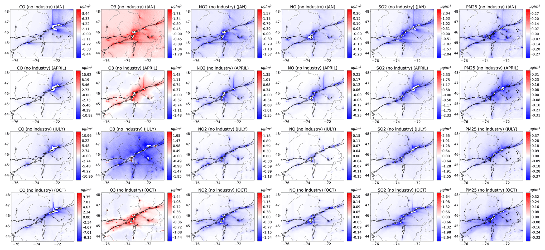
Figure 12Monthly averaged plots (January, April, July, and October, from top to bottom) showing the model with full emissions subtracted from a run with no industrial emissions at the 3 km resolution for (from left to right) CO, O3, NO2, NO, SO2, and PM2.5. The X's indicate NPRI emissions corresponding to each species, except for O3, NO, and NO2, where NOx emission sites were used. All units are in µg m−3.
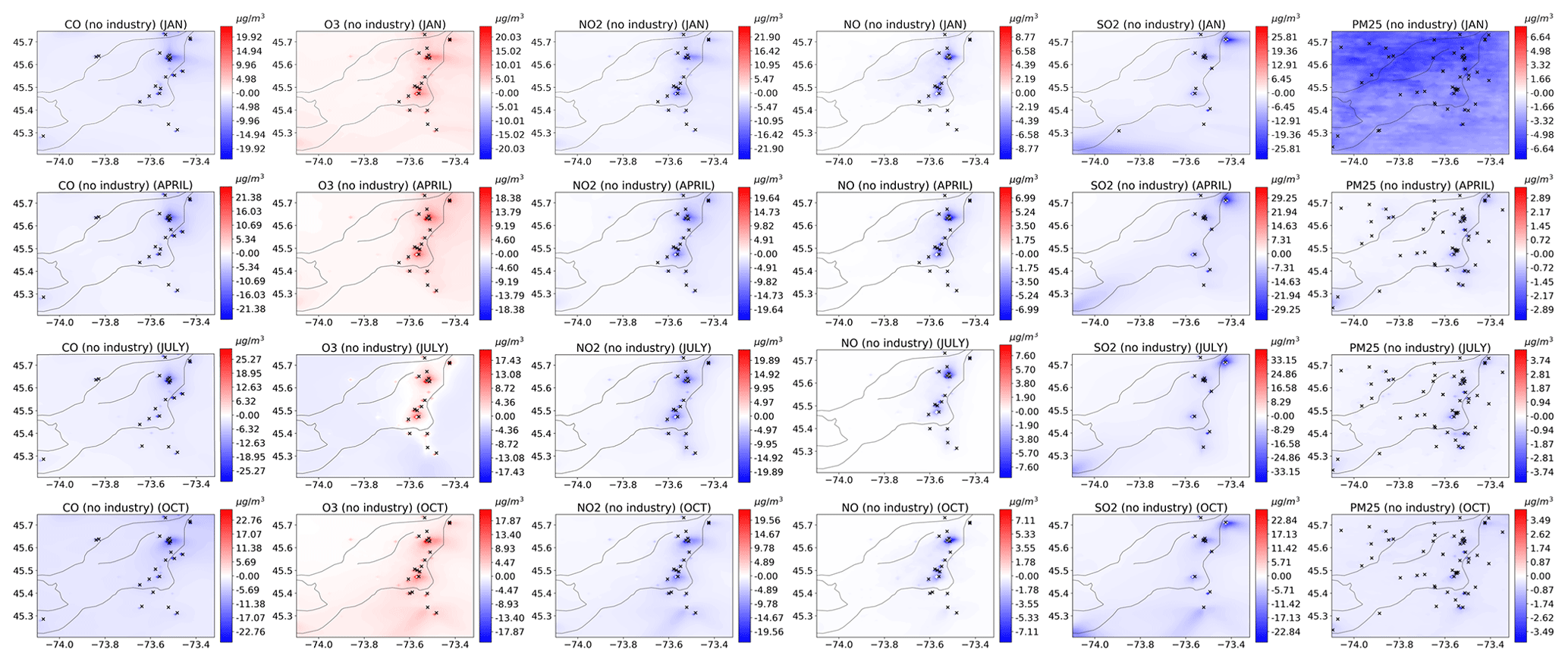
Figure 13Monthly averaged plots (January, April, July, and October, from top to bottom) showing the model with full emissions subtracted from a run with no industrial emissions at the 1 km resolution over Montréal for (from left to right) CO, O3, NO2, NO, SO2, and PM2.5. The X's indicate NPRI emissions corresponding to each species, except for O3, NO, and NO2, where NOx emission sites were used. All units are in µg m−3.
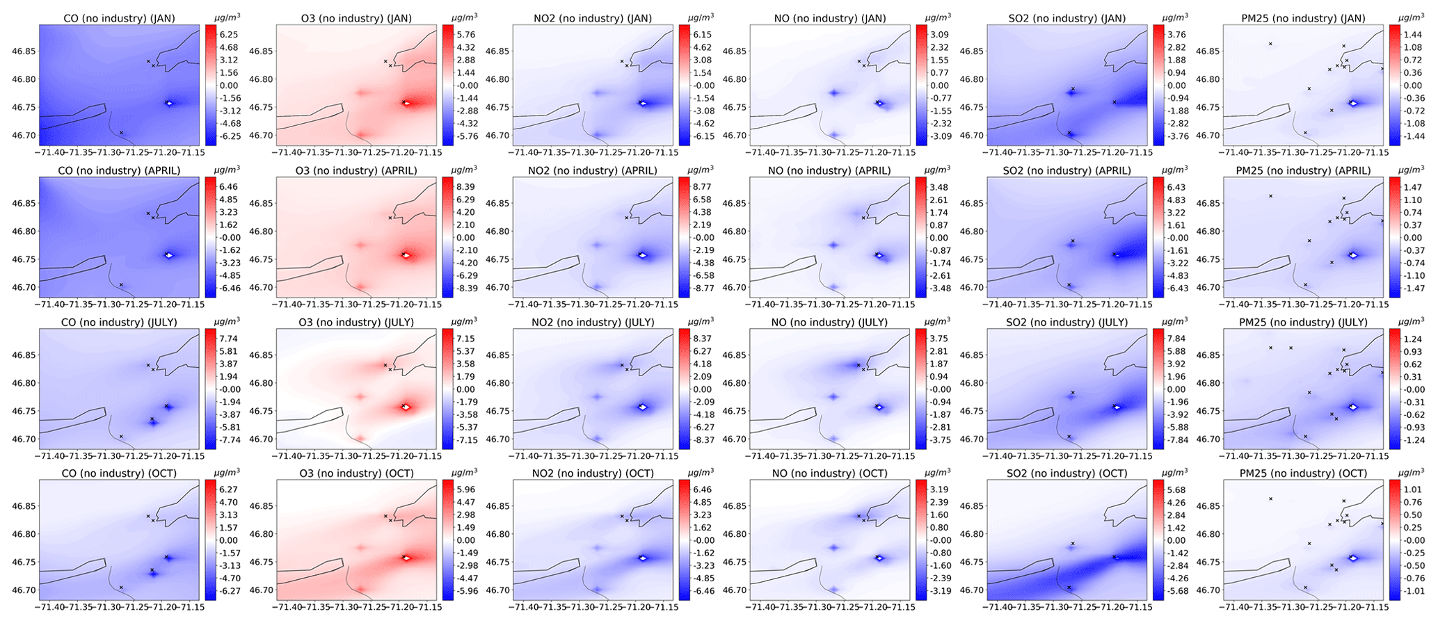
Figure 14Monthly averaged plots (January, April, July, and October, from top to bottom) showing the model with full emissions subtracted from a run with no industrial emissions at the 1 km resolution over Québec for (from left to right) CO, O3, NO2, NO, SO2, and PM2.5. The X's indicate NPRI emissions corresponding to each species, except for O3, NO, and NO2, where NOx emission sites were used. All units are in µg m−3.
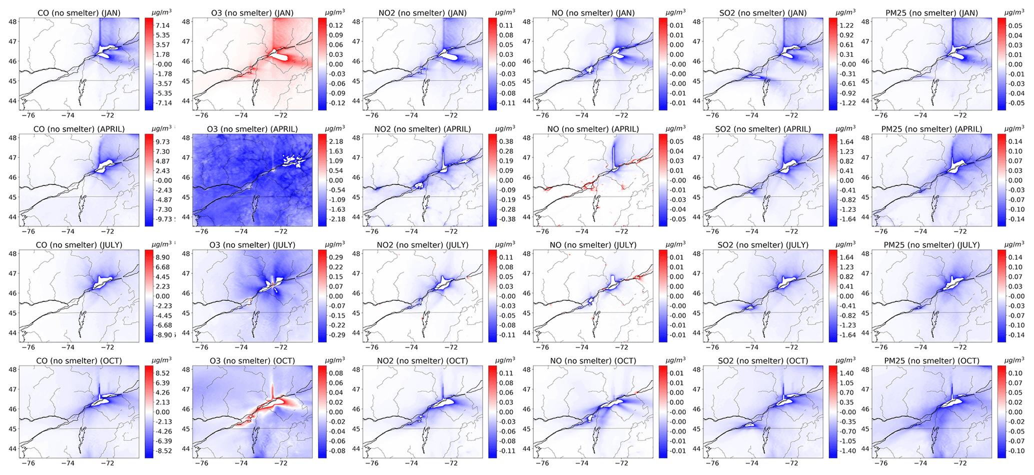
Figure 15Monthly averaged plots (January, April, July, and October, from top to bottom) showing the model with full emissions subtracted from a run with no emissions from smelter and refinery industries at the 3 km resolution for (from left to right) CO, O3, NO2, NO, SO2, and PM2.5. All units are in µg m−3.
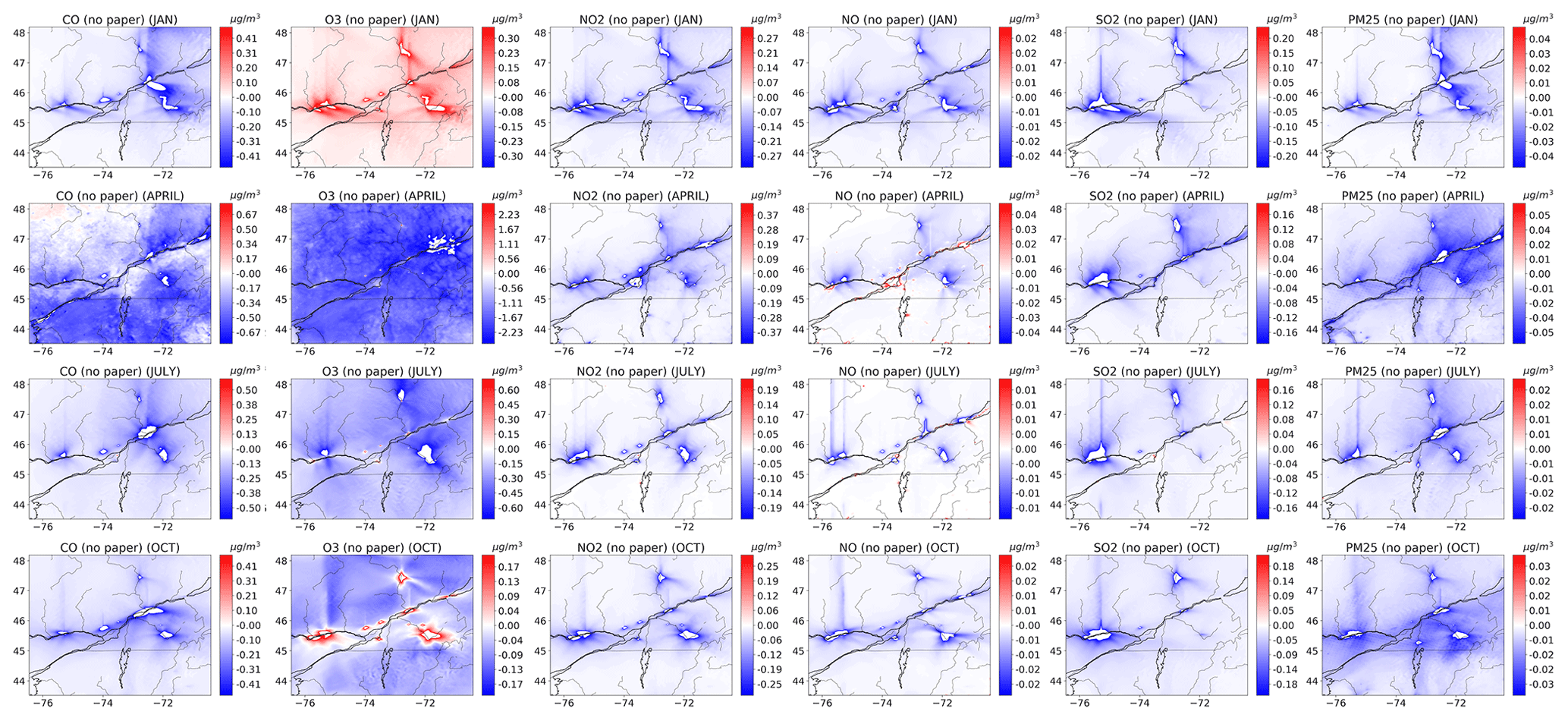
Figure 16Monthly averaged plots (January, April, July, and October, from top to bottom) showing the model with full emissions subtracted from a run with no emissions from paper and pulp industries at the 3 km resolution for (from left to right) CO, O3, NO2, NO, SO2, and PM2.5. All units are in µg m−3.
In this study, the Polyphemus Polair3D CTM was run over Quebec, Canada, to assess the model's capability in predicting key air pollutant species over the region at the ground (surface) level model, at seasonal temporal scales, and at regional spatial scales. This represents a novel use of the Polair3D model; this study presents, to the best of our knowledge, the first time the Polair3D model was used over Quebec, Canada, with a long-enough modeling period to capture seasonal effects and a large modeling domain spanning urban to rural areas.
The model was run in three nested domains; the largest and coarsest-resolution domain was roughly 9 km by 9 km grid-cell resolution (edges), and within it, a smaller 3 km by 3 km resolution was run, and lastly 1 km by 1 km resolution runs were performed over the cities of Montréal and Québec. The model was run with the meteorology field from the pre-run WRF, and the SMOKE emissions-processing system was used to prepare the emissions input files. Canadian and United States (US) emissions in the domain were calculated based on SMOKE-ready formats of the Canadian emission inventory and US National Emissions Inventory, along with their temporal allocation and chemical speciation data. Spatial allocations for the three nested domains were generated using both Canadian and US spatial allocator inputs. The model was run for four seasons from 2018, with 4 weeks per season (January for winter, April for spring, July for summer, and October for fall), for a total of 16 weeks of model data. Spin-up was done for 1 week for each run. Boundary conditions for the outermost domain and the initial conditions for each of the runs were derived from CAM-Chem assimilated data.
The model at the 3 km resolution showed varying levels of performance for different pollutant species. The model at both the 3 km and the 1 km resolution struggled to capture high-frequency temporal variability, at least at the surface, and showed large variabilities in correlation and bias from site to site. Doing a site-wide analysis (i.e., comparing monthly averages across all sites) suggested that the model is better at capturing the spatial variability and seasonal effects rather than hour-by-hour or day-to-day temporal variability for a fixed location.
When comparing the biases and correlation at a site-wide scale, the higher-resolution 1 km runs did not result in strictly better performance; when analyzing the same sites (i.e., restricting the 3 km analysis to the NAPS sites seen in the smaller 1 km run), the 3 km model showed slightly higher correlation for O3, NO2, and NO, and while SO2 and PM2.5 showed increases in correlation, the differences were not large (CO correlation was the same for both cases). Examining the model performance site by site showed similar results; running the model at an increased resolution may be an effective way to downscale the data, but it does not appear to make the simulation more temporally accurate. Comparing against CANUE national LUR NO2 showed high correlations, ranging between R=0.91 (in July) and 0.86 (in October). At the 1 km resolution, another analysis was conducted, separating daytime and nighttime data; one noteworthy result from this analysis is that the slope was higher during the day for all species except SO2. Correlation was higher for CO, O3, NO, and PM2.5 and was slightly lower for NO2 and SO2. Furthermore, O3, a secondary pollutant that is created and destroyed photochemically and thus heavily affected by sunlight, showed higher correlation during the day than during the night, while at the same time it showed large underestimation biases during the night. This suggests that the model is capable of modeling O3 during the day but struggles to simulate the background O3 during the night where photochemical reactions are low and/or nonexistent. For CO, correlation was significantly higher during the day than during the night (R=0.91 versus −0.69), although the difference was less extreme when looking at individual months.
A test scenario, where the model was run without industrial emissions, showed that the model generally captures the spatial variability of industrial emissions and captures spatial gradients related to proximity to industrial sources. While industrial contribution is not high overall, large spatial gradients were seen in its contributions, even at intracity scales.
The performance of the Polair3D model over Quebec was in line with other models like GEM-MACH over Canada, albeit with higher biases overall, and comparable to the performance of Polair3D over Europe, where the model was developed. For key air pollutants such as O3 and NO2, Polair3D showed similar correlations and comparable biases.
The Polyphemus platform, including the Polair3D CTM used in this study, is available at https://doi.org/10.5281/zenodo.10067062 (Kim et al., 2023).
SY ran the model with emissions inventories prepared by SMG. All authors contributed valuable discussions to this study. SY wrote the paper with input from all authors.
The contact author has declared that none of the authors has any competing interests.
Publisher's note: Copernicus Publications remains neutral with regard to jurisdictional claims made in the text, published maps, institutional affiliations, or any other geographical representation in this paper. While Copernicus Publications makes every effort to include appropriate place names, the final responsibility lies with the authors.
This work was funded by Health Canada's Addressing Air Pollution Horizontal Initiative.
This research has been supported by Health Canada (grant no. 4500416078).
This paper was edited by Jason Williams and reviewed by two anonymous referees.
Bartholomé, E. and Belward, A. S.: GLC2000: a new approach to global land cover mapping from Earth observation data, Int. J. Remote Sens., 26, 1959–1977, https://doi.org/10.1080/01431160412331291297, 2005. a
Batisse, E., Goudreau, S., Baumgartner, J., and Smargiassi, A.: Socio-economic inequalities in exposure to industrial air pollution emissions in Quebec public schools, Can. J. Publ. He., 108, e503–e509, https://doi.org/10.17269/CJPH.108.6166, 2017. a
Boutahar, J., Lacour, S., Mallet, V., Quélo, D., Roustan, Y., and Sportisse, B.: Development and validation of a fully modular platform for numerical modelling of air pollution: POLAIR, Int. J. Environ. Pollut., 22, 17–28, 2004. a
Brand, A., McLean, K. E., Henderson, S. B., Fournier, M., Liu, L., Kosatsky, T., and Smargiassi, A.: Respiratory hospital admissions in young children living near metal smelters, pulp mills and oil refineries in two Canadian provinces, Environ. Int., 94, 24–32, https://doi.org/10.1016/j.envint.2016.05.002, 2016. a
Buteau, S., Shekarrizfard, M., Hatzopolou, M., Gamache, P., Liu, L., and Smargiassi, A.: Air pollution from industries and asthma onset in childhood: A population-based birth cohort study using dispersion modeling, Environ. Res., 185, 109180, https://doi.org/10.1016/j.envres.2020.109180, 2020. a
Chen, F. and Dudhia, J.: Coupling an Advanced Land Surface–Hydrology Model with the Penn State–NCAR MM5 Modeling System. Part I: Model Implementation and Sensitivity, Mon. Weather Rev., 129, 569–585, https://doi.org/10.1175/1520-0493(2001)129<0569:CAALSH>2.0.CO;2, 2001. a
Chen, F., Kusaka, H., Bornstein, R., Ching, J., Grimmond, C. S. B., Grossman-Clarke, S., Loridan, T., Manning, K. W., Martilli, A., Miao, S., Sailor, D., Salamanca, F. P., Taha, H., Tewari, M., Wang, X., Wyszogrodzki, A. A., and Zhang, C.: The integrated WRF/urban modelling system: development, evaluation, and applications to urban environmental problems, Int. J. Climatol., 31, 273–288, https://doi.org/10.1002/joc.2158, 2011. a
Chen, J., Pendlebury, D., Gravel, S., Stroud, C., Ivanova, I., DeGranpré, J., and Plummer, D.: Development and Current Status of the GEM-MACH-Global Modelling System at the Environment and Climate Change Canada, in: Air Pollution Modeling and its Application XXVI, edited by: Mensink, C., Gong, W., and Hakami, A., 107–112, Springer International Publishing, Cham, 2020. a
Chen, S.-H. and Sun, W.-Y.: A One-dimensional Time Dependent Cloud Model, J. Meteorol. Soc. Jpn. Ser. II, 80, 99–118, https://doi.org/10.2151/jmsj.80.99, 2002. a
CMAS-DB: Surrogate Tools DB, https://www.cmascenter.org/surrogate_tools_db/, last access: 28 February 2023. a
CMAS-SA: SPATIAL ALLOCATOR- SA-TOOLS, https://www.cmascenter.org/sa-tools/, last access: 28 February 2023. a
CMAS-SMOKE: CMAS: Community Modeling and Analysis System, https://www.cmascenter.org/smoke/, last access: 20 February 2023. a
DMTI Spatial Inc.: CanMap Content Suite, [CanMap Postal Suite], v2015.3, https://doi.org/11272.1/AB2/WZOPIP, 2015. a, b
EMEP/EEA: EMEP/EEA air pollutant emission inventory guidebook, https://www.eea.europa.eu//publications/emep-eea-guidebook-2019 (last access: 28 February 2023), 2019. a
Emery, C., Liu, Z., Russell, A. G., Odman, M. T., Yarwood, G., and Kumar, N.: Recommendations on statistics and benchmarks to assess photochemical model performance, J. Air Waste Manage. A., 67, 582–598, https://doi.org/10.1080/10962247.2016.1265027, 2017. a, b
Environment and Canada, C. C.: Information archivée dans le Web | Information Archived on the Web, https://publications.gc.ca/collections/collection_2017/eccc/En81-26-2015-eng.pdf (last access: 28 February 2023), 2017. a
EPA-CMAQ: Meteorology – Chemistry Interface Processor, https://www.epa.gov/cmaq/meteorology-chemistry-interface-processor, last access: 28 February 2023. a
EPA: Emissions Modeling Platforms: EPA: Emissions Modeling Platforms, https://www.epa.gov/air-emissions-modeling/emissions-modeling-platforms, last access: 22 February 2023. a, b
GBD 2015 Risk Factors Collaborators: Global, regional, and national comparative risk assessment of 79 behavioural, environmental and occupational, and metabolic risks or clusters of risks, 1990-2015: a systematic analysis for the Global Burden of Disease Study 2015, The Lancet, 388, 1659–1724, https://doi.org/10.1016/S0140-6736(16)31679-8, 2016. a
Grell, G. A. and Dévényi, D.: A generalized approach to parameterizing convection combining ensemble and data assimilation techniques, Geophys. Res. Lett., 29, 38-1–38-4, https://doi.org/10.1029/2002GL015311, 2002. a
Health Canada: Outdoor air pollution and health: Overview, https://www.canada.ca/en/health-canada/services/air-quality/outdoor-pollution-health.html (last access: 7 March 2023), 2022a. a
Health Canada: HEALTH IMPACTS OF TRAFFIC-RELATED AIR POLLUTION IN CANADA, Health Canada, Ottawa, Ontario, Canada, ISBN 978-0-660-40966-5, 2022b. a, b, c
Hystad, P., Setton, E., Cervantes, A., Poplawski, K., Deschenes, S., Brauer, M., van Donkelaar, A., Lamsal, L., Martin, R., Jerrett, M., and Demers, P.: Creating National Air Pollution Models for Population Exposure Assessment in Canada, Environ. Health Persp., 119, 1123–1129, https://doi.org/10.1289/ehp.1002976, 2011. a, b
Iacono, M. J., Delamere, J. S., Mlawer, E. J., Shephard, M. W., Clough, S. A., and Collins, W. D.: Radiative forcing by long-lived greenhouse gases: Calculations with the AER radiative transfer models, J. Geophys. Res.-Atmos., 113, D13, https://doi.org/10.1029/2008JD009944, 2008. a
Janjić, Z. I.: The Step-Mountain Eta Coordinate Model: Further Developments of the Convection, Viscous Sublayer, and Turbulence Closure Schemes, Mon. Weather Rev., 122, 927–945, https://doi.org/10.1175/1520-0493(1994)122<0927:TSMECM>2.0.CO;2, 1994. a
Jeong, C., McGuire, M. L., Herod, D., Dann, T., Dabek-Zlotorzynska, E., Wang, D., Ding, L., Celo, V., Mathieu, D., and Evans, G.: Receptor model based identification of PM2.5 sources in Canadian cities, Atmos. Pollut. Res., 2, 158–171, https://doi.org/10.5094/APR.2011.021, 2011. a
Kim, Y., Wu, Y., Seigneur, C., and Roustan, Y.: Multi-scale modeling of urban air pollution: development and application of a Street-in-Grid model (v1.0) by coupling MUNICH (v1.0) and Polair3D (v1.8.1), Geosci. Model Dev., 11, 611–629, https://doi.org/10.5194/gmd-11-611-2018, 2018. a
Kim, Y., Sartelet, K., and Roustan, Y.: Polyphemus: Air quality modeling system, Zenodo [code and data set], https://doi.org/10.5281/zenodo.10067062, 2023. a, b
Krzyzanowski, J.: The Importance of Policy in Emissions Inventory Accuracy— A Lesson from British Columbia, Canada, J. Air Waste Manage. A., 59, 430–439, https://doi.org/10.3155/1047-3289.59.4.430, 2009. a
Lecœur, È. and Seigneur, C.: Dynamic evaluation of a multi-year model simulation of particulate matter concentrations over Europe, Atmos. Chem. Phys., 13, 4319–4337, https://doi.org/10.5194/acp-13-4319-2013, 2013. a
Liu, Y., Geng, X., Smargiassi, A., Fournier, M., Gamage, S. M., Zalzal, J., Yamanouchi, S., Torbatian, S., Minet, L., Hatzopoulou, M., Buteau, S., Laouan-Sidi, E.-A., and Liu, L.: Changes in industrial air pollution and the onset of childhood asthma in Quebec, Canada, Environ. Res., 243, 117831, https://doi.org/10.1016/j.envres.2023.117831, 2024. a
Lugon, L., Sartelet, K., Kim, Y., Vigneron, J., and Chrétien, O.: Nonstationary modeling of NO2, NO and NOx in Paris using the Street-in-Grid model: coupling local and regional scales with a two-way dynamic approach, Atmos. Chem. Phys., 20, 7717–7740, https://doi.org/10.5194/acp-20-7717-2020, 2020. a
Makar, P., Gong, W., Hogrefe, C., Zhang, Y., Curci, G., Žabkar, R., Milbrandt, J., Im, U., Balzarini, A., Baró, R., Bianconi, R., Cheung, P., Forkel, R., Gravel, S., Hirtl, M., Honzak, L., Hou, A., Jiménez-Guerrero, P., Langer, M., Moran, M., Pabla, B., Pérez, J., Pirovano, G., San José, R., Tuccella, P., Werhahn, J., Zhang, J., and Galmarini, S.: Feedbacks between air pollution and weather, part 2: Effects on chemistry, Atmos. Environ., 115, 499–526, https://doi.org/10.1016/j.atmosenv.2014.10.021, 2015. a
Mallet, V. and Sportisse, B.: 3-D chemistry-transport model Polair: numerical issues, validation and automatic-differentiation strategy, Atmos. Chem. Phys. Discuss., 4, 1371–1392, https://doi.org/10.5194/acpd-4-1371-2004, 2004. a
Mallet, V., Quélo, D., Sportisse, B., Ahmed de Biasi, M., Debry, É., Korsakissok, I., Wu, L., Roustan, Y., Sartelet, K., Tombette, M., and Foudhil, H.: Technical Note: The air quality modeling system Polyphemus, Atmos. Chem. Phys., 7, 5479–5487, https://doi.org/10.5194/acp-7-5479-2007, 2007. a, b
Mesinger, F., DiMego, G., Kalnay, E., Mitchell, K., Shafran, P. C., Ebisuzaki, W., Jović, D., Woollen, J., Rogers, E., Berbery, E. H., Ek, M. B., Fan, Y., Grumbine, R., Higgins, W., Li, H., Lin, Y., Manikin, G., Parrish, D., and Shi, W.: North American Regional Reanalysis, B. Am. Meteorol. Soc., 87, 343–360, https://doi.org/10.1175/BAMS-87-3-343, 2006. a
Minet, L., Wang, A., and Hatzopoulou, M.: Health and Climate Incentives for the Deployment of Cleaner On-Road Vehicle Technologies, Environ. Sci. Technol., 55, 6602–6612, https://doi.org/10.1021/acs.est.0c07639, 2021. a, b, c
Ministry of the Environment and Climate Change: Air Quality in Ontario: 2016 Report, Distributed by the Ministry of the Environment, Conservation and Parks (current name), Toronto, Ontario, Canada, 2016. a
NAPS: National Air Pollution Surveillance (NAPS) Program, https://open.canada.ca/data/en/dataset/1b36a356-defd-4813-acea-47bc3abd859b (last access: 7 March 2023), 2016. a, b
NCAR: Weather Research & Forecasting Model (WRF), https://www.mmm.ucar.edu/models/wrf (last access: 7 March 2023), 2023. a
Pourchet, A., Mallet, V., Quélo, D., and Sportisse, B.: Some numerical issues in Chemistry-Transport Models – a comprehensive study with the Polyphemus/Polair3D platform, Tech. Rep. 26, CEREA, 2005. a
Rai, P. K.: Chapter Two – Adverse Health Impacts of Particulate Matter, in: Biomagnetic Monitoring of Particulate Matter, edited by: Rai, P. K., 15–39, Elsevier, ISBN 978-0-12-805135-1, https://doi.org/10.1016/B978-0-12-805135-1.00002-0, 2016. a
Russell, M., Hakami, A., Makar, P. A., Akingunola, A., Zhang, J., Moran, M. D., and Zheng, Q.: An evaluation of the efficacy of very high resolution air-quality modelling over the Athabasca oil sands region, Alberta, Canada, Atmos. Chem. Phys., 19, 4393–4417, https://doi.org/10.5194/acp-19-4393-2019, 2019. a, b, c, d
Sartelet, K., Couvidat, F., Wang, Z., Flageul, C., and Kim, Y.: SSH-Aerosol v1.1: A Modular Box Model to Simulate the Evolution of Primary and Secondary Aerosols, Atmosphere, 11, 525, https://doi.org/10.3390/atmos11050525, 2020. a
Sartelet, K. N., Boutahar, J., Quélo, D., Coll, I., Plion, P., and Sportisse, B.: Development and validation of a 3D Chemistry-Transport Model, Polair3D, by comparison with data from ESQUIF campaign, in: Proceedings of the 6th Gloream workshop: Global and regional atmospheric modelling, 140–146, 1 January 2002, Aveiro, Portugal, 2002. a
Sartelet, K. N., Couvidat, F., Seigneur, C., and Roustan, Y.: Impact of biogenic emissions on air quality over Europe and North America, Atmos. Environ., 53, 131–141, https://doi.org/10.1016/j.atmosenv.2011.10.046, 2012. a, b, c
Sassi, M., Zhang, J., and Moran, M. D.: 2015 SMOKE-Ready Canadian Air Pollutant Emission Inventory (APEI) Package version 1, Zenodo [code], https://doi.org/10.5281/zenodo.4883639, 2021. a
Smargiassi, A., Goldberg, M. S., Wheeler, A. J., Plante, C., Valois, M.-F., Mallach, G., Kauri, L. M., Shutt, R., Bartlett, S., Raphoz, M., and Liu, L.: Associations between personal exposure to air pollutants and lung function tests and cardiovascular indices among children with asthma living near an industrial complex and petroleum refineries, Environ. Res., 132, 38–45, https://doi.org/10.1016/j.envres.2014.03.030, 2014. a
Stroud, C. A., Ren, S., Zhang, J., Moran, M. D., Akingunola, A., Makar, P. A., Munoz-Alpizar, R., Leroyer, S., Bélair, S., Sills, D., and Brook, J. R.: Chemical Analysis of Surface-Level Ozone Exceedances during the 2015 Pan American Games, Atmosphere, 11, 572, https://doi.org/10.3390/atmos11060572, 2020. a, b, c
Thouron, L., Seigneur, C., Kim, Y., Legorgeu, C., Roustan, Y., and Bruge, B.: Simulation of trace metals and PAH atmospheric pollution over Greater Paris: Concentrations and deposition on urban surfaces, Atmos. Environ., 167, 360–376, https://doi.org/10.1016/j.atmosenv.2017.08.027, 2017. a
Tilmes, S., Lamarque, J.-F., Emmons, L. K., Kinnison, D. E., Ma, P.-L., Liu, X., Ghan, S., Bardeen, C., Arnold, S., Deeter, M., Vitt, F., Ryerson, T., Elkins, J. W., Moore, F., Spackman, J. R., and Val Martin, M.: Description and evaluation of tropospheric chemistry and aerosols in the Community Earth System Model (CESM1.2), Geosci. Model Dev., 8, 1395–1426, https://doi.org/10.5194/gmd-8-1395-2015, 2015. a
van Donkelaar, A., Hammer, M. S., Bindle, L., Brauer, M., Brook, J. R., Garay, M. J., Hsu, N. C., Kalashnikova, O. V., Kahn, R. A., Lee, C., Levy, R. C., Lyapustin, A., Sayer, A. M., and Martin, R. V.: Monthly Global Estimates of Fine Particulate Matter and Their Uncertainty, Environ. Sci. Technol., 55, 15287–15300, https://doi.org/10.1021/acs.est.1c05309, 2021. a, b
Wallington, T. J., Anderson, J. E., Dolan, R. H., and Winkler, S. L.: Vehicle Emissions and Urban Air Quality: 60 Years of Progress, Atmosphere, 13, 650, https://doi.org/10.3390/atmos13050650, 2022. a
Weichenthal, S., Pinault, L. L., and Burnett, R. T.: Impact of Oxidant Gases on the Relationship between Outdoor Fine Particulate Air Pollution and Nonaccidental, Cardiovascular, and Respiratory Mortality, Sci. Rep., 7, 16401, https://doi.org/10.1038/s41598-017-16770-y, 2017. a