HGS-PDAF (version 1.0): a modular data assimilation framework for an integrated surface and subsurface hydrological model

This article describes a modular ensemble-based data assimilation (DA) system which is developed for an integrated surface–subsurface hydrological model. The software environment for DA is the Parallel Data Assimilation Framework (PDAF), which provides various assimilation algorithms like the ensemble Kalman filters, non-linear filters, 3D-Var and combinations among them. The integrated surface–subsurface hydrological model is HydroGeoSphere (HGS), a physically based modelling software for the simulation of surface and variably saturated subsurface flow, as well as heat and mass transport. The coupling and capabilities of the modular DA system are described and demonstrated using an idealised model of a geologically heterogeneous alluvial river–aquifer system with drinking water production via riverbank filtration. To demonstrate its modularity and adaptability, both single and multivariate assimilations of hydraulic head and soil moisture observations are demonstrated in combination with individual and joint updating of multiple simulated states (i.e. hydraulic heads and water saturation) and model parameters (i.e. hydraulic conductivity). With the integrated model and this modular DA framework, we have essentially developed the hydrologically and DA-wise robust toolbox for developing the basic model for operational management of coupled surface water–groundwater resources.

1 Introduction

Numerical hydrological models are appropriate decision support tools for water resource management, as they can be used to better understand and predict complex hydrological systems that are dynamically evolving as a result of natural and anthropogenic stresses. When it comes to managing shallow groundwater systems, integrated surface–subsurface hydrological models (ISSHMs) (Sebben et al., 2013) are essential as they simulate all the components of the hydrological cycle and their feedback mechanisms within a single framework (Doherty and Moore, 2020; Islam, 2011; Paniconi and Putti, 2015). ISSHMs provide a physically based and hydrologically consistent simulation of water fluxes across the entire hydrological system (Simmons et al., 2020). This makes ISSHMs robust tools for the simulation of water quantity and quality and thus for supporting the prospective management of water resources (Yang et al., 2021; Paudel and Benjankar, 2022; Du et al., 2012; Burek et al., 2020; Belleflamme et al., 2023). Furthermore, ISSHMs also allow the potential impacts of climate change and human activity on the natural water system to be studied (Wada et al., 2017). Examples of such ISSHMs include MIKE-SHE (Refsgaard et al., 1995), InHM (VanderKwaak and Loague, 2001), IHM (Ross et al., 2005), ParFlow (Kollet and Maxwell, 2006), CATHY (Camporese et al., 2010) and HydroGeoSphere (HGS; Brunner and Simmons, 2012; Aquanty, 2020). As with any modelling approach, complex ISSHMs necessitate the minimisation of uncertainty in both model parameters and predictions. This is ideally achieved through inverse estimation of model parameters using available direct and indirect observations, facilitated by some form of data assimilation. Model parameters in ISSHMs generally represent the many different physically and sometimes also the biogeochemically relevant hydraulic and hydrological properties of the surface and subsurface, and these parameters are typically spatially and sometimes also temporally highly heterogeneous. Moreover, the true values of these parameters are usually not precisely measurable, and any hydrological modelling effort, be it based on an elaborate ISSHM or even a simple bucket-type model, inevitably starts off with considerable prior uncertainty (Moges et al., 2020). In addition, model forcing data and model structure are associated with uncertainty, and, unless they are reduced and/or appropriately accounted for, all these uncertainties have the potential to significantly limit the reliability of (integrated) numerical models. Thus, the quantification and reduction of model uncertainty is a critical step for any decision-based hydrological model (Anderson et al., 2015) and important for both research and for operational modelling efforts (Liu and Gupta, 2007). While different methods exist, one of the most robust approaches to quantify and reduce model uncertainties is through data assimilation (DA) (Fan et al., 2022). DA is used widely in oceanography and meteorology (see Hoteit et al., 2018; Ghil and Malanotte-Rizzoli, 1991), particularly for global reanalysis (Baatz et al., 2021) and operational weather forecasting (Navon, 2009; Hu et al., 2023), where DA frameworks integrate measurements in near-real time into models and continuously correct for model deviations from the “true” system states. In recent years, DA has also been applied more frequently to continental hydrological systems, especially for experimental studies with physically based models and operational flood forecasting (Camporese and Girotto, 2022). By continuously incorporating real-time information from ground sensors and remote sensing, as well as weather forecasts, into hydrological models via DA, the uncertainties of hydrological model predictions could be significantly reduced and operational short-term forecasts improved (Di Marco et al., 2021).

So far, studies on the implementation and development of DA for coupled surface–subsurface hydrological system modelling, particularly via ISSHMs, are very limited. A successful implementation was demonstrated for the first time by Paniconi et al. (2003), who applied the simple DA method of nudging to the simplified version of the physically based surface–subsurface model CATHY (Camporese et al., 2010). It was shown that through the assimilation of soil moisture observations, the hydrological simulations improved significantly and for little additional computational cost. After more experimental DA examples were developed with CATHY (e.g. Camporese et al., 2009b, a), DA started to be explored also for use with other ISSHMs. Kurtz et al. (2016) developed a data assimilation framework for the Terrestrial System Modelling Platform (TerrSysMP) (Shrestha et al., 2014) using the DA software Parallel Data Assimilation Framework (PDAF) (Nerger et al., 2005). TerrSysMP itself is a modular Earth system model consisting of the atmospheric model COSMO (Baldauf et al., 2011), the land surface model CLM (Community Land Model; Oleson et al., 2004) and the ISSHM ParFlow (Kollet and Maxwell, 2006), all coupled via OASIS-MCT (Valcke, 2013). The data assimilation framework TerrSysMP-PDAF allows the assimilation of pressure heads and soil moisture measurements into the ISSHM ParFlow and the land surface model CLM via different assimilation algorithms as provided by PDAF. Similarly, an ensemble Kalman filter (EnKF)-based data assimilation system for the physically based ISSHM HydroGeoSphere, EnKF-HGS, was developed by Kurtz et al. (2017), which allowed the assimilation of hydraulic heads with joint updating of both hydraulic heads and hydraulic conductivities. Based on EnKF-HGS, Tang et al. (2017, 2018) assimilated hydraulic head observations for the joint estimation of states (hydraulic heads and surface water discharge) and parameters (hydraulic conductivities of an alluvial aquifer and a riverbed). Compared to ParFlow, which is the ISSHM in TerrSysMP-PDAF and which is best suited for the simulation of larger-scale interactions between the subsurface, the land surface and the atmosphere (Condon and Maxwell, 2019), HGS is more suited for local-scale surface–subsurface interactions and the explicit and efficient simulation of abstraction schemes in riverbank filtration contexts, reactive transport processes, managed aquifer recharge systems, geothermal systems, agricultural drainage (e.g. tile drain) and irrigation infrastructure (Alvarado et al., 2022; Boico et al., 2022; Schilling et al., 2022; Delottier et al., 2022b).

Up to now, only the EnKF was implemented as a data assimilation algorithm for HGS (via EnKF-HGS), and the coupling was neither modular nor user-friendly and is thus not suited for operational implementations. A better solution than coupling a single DA algorithm to an ISSHM is the coupling of existing DA software that offers a suite of different assimilation algorithms to choose from and is modular with respect to the choice of states, parameters and observations that should be updated or considered for DA. As a toolbox tailored towards numerical modelling, PDAF offers such a modular choice of widely used DA algorithms and supports both single and multivariate assimilation of different types of observations, as well as single or joint state and parameter updating. PDAF also facilitates the addition of novel assimilation algorithms which are not yet included. Owing to its modular design, PDAF makes it very easy to switch between different assimilation methods without the need for additional coding. Last but not least, the different algorithms are not only fully implemented and optimised but also parallelised, which is a key aspect for the continental-scale hydrological modelling conducted with the TerrSysMP-PDAF platform.

With the aim to provide a DA framework for operational real-time simulations of water quality and quantity in complex systems for which ISSHMs are typically the ideal decision-based modelling tools (e.g. riverbank filtration wellfields, managed aquifer recharge schemes or agricultural systems), we have developed a highly modular DA framework for ISSHMs based on PDAF and HGS. The coupled framework, called HGS-PDAF, is designed to allow updating of integrated flow and transport simulations and includes the following key features:

1. the most up-to-date and continuously maintained collection of data assimilation algorithms, including the ensemble Kalman filter and its established variants, the ensemble smoother, the three-dimensional variational method, and the hybrid ensemble–variational method;

2. a modular tool to handle different types of observation data, which enables it to assimilate one or multiple types of observations simultaneously, currently programmed for hydraulic heads, soil moisture and solute concentration measurements;

3. a modular tool to handle different model states and parameters in HGS-PDAF allowing individual or joint updates of one or multiple states (currently: hydraulic heads, soil water saturation and solute concentration) and parameter types (currently: hydraulic conductivity);

4. an open-source code repository, which includes the source code, an example test case, and documentation on the use of the code and the execution of the example.

Here, the structure and modules of HGS-PDAF are presented, alongside its capabilities and its performance on a multivariate, joint state-parameter DA example based on a synthetic alluvial riverbank filtration wellfield model. The structure of this paper is as follows: Sect. 2 describes the structure of the ISSHM HGS, the DA software PDAF and the specific DA algorithm used in the illustrative example. Section 3 presents the coupled DA framework HGS-PDAF. Section 4 illustrates the implementation and performance of HGS-PDAF on the synthetic test case. The potential for HGS-PDAF to serve as a DA framework for different scientific and management applications in the water sector and avenues for further developments and improvements to HGS-PDAF are discussed in Sect. 5. The source code of HGS-PDAF, a manual and the presented example test case are available freely via https://doi.org/10.5281/zenodo.10000886 (Tang et al., 2023).

2 Hydrological model and data assimilation method

2.1 General overview of the ISSHM HydroGeoSphere

HGS (Aquanty, Inc.) is an integrated surface–subsurface hydrological model (ISSHM) that was originally developed by Therrien and Sudicky (1996) and can be used to simulate fully coupled surface water and variably saturated subsurface flow, as well as heat and mass transport (Brunner and Simmons, 2012; Aquanty, 2020). In HGS, surface water flow is simulated using the two-dimensional diffusion wave equation and (variably saturated) subsurface flow using the three-dimensional Richards equation. The surface and subsurface domains are fully coupled in a physically consistent manner, enabling dynamic, two-way feedbacks between these two domains. This is achieved by simultaneously solving the surface and subsurface flow and transport equations in one single system of equations. Owing to its versatility, HGS has been used to study surface–subsurface flow and transport in complex, heterogeneous hydro(geo)logical systems (e.g. Ala-Aho et al., 2017; Schilling et al., 2014, 2017; Thornton et al., 2022). It has also been used to assess the potential impacts of, and responses to, climate change on hydrological processes at regional scales (Nagare et al., 2023; Erler et al., 2019; Delottier et al., 2022a; Cochand et al., 2019); to explore the dynamics of coastal groundwater flooding under a dual-aquifer configuration (Tajima et al., 2023); in geophysics to inversely estimate the hydraulic conductivity (Sun et al., 2023) and in the context of supporting hydraulic tomography (Wang and Illman, 2023); and to extract and estimate groundwater recharge (Gong et al., 2023). Importantly, a recent study by Delottier et al. (2022b) has enhanced HGS such that it can now explicitly handle reactive (gas) tracers in transient solute transport simulations under variably saturated conditions.

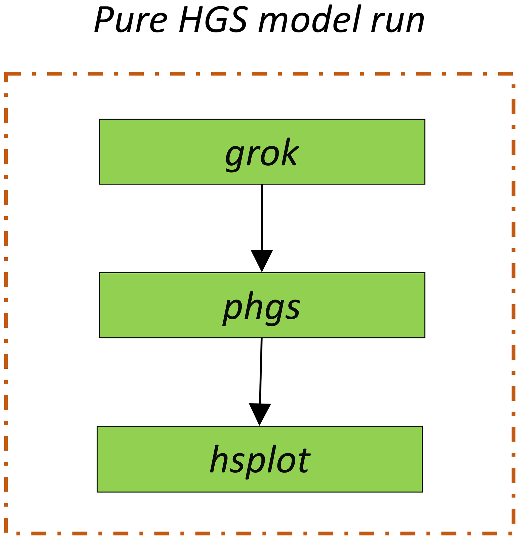
HGS has three key executables: grok, phgs and hsplot. grok is the pre-processing executable which compiles the prefix.grok file containing the model definition and setup information. It prepares all the information needed for HGS to run simulations. phgs is the main executable for running a serial or parallel forward numerical simulation with HGS. hsplot is the post-processing executable that converts the model output files into a readable format that can be later visualised, for example, by Tecplot (Tecplot, Inc.) or the open-source tool ParaView (Kitware, Inc.). Thus, grok must be run before phgs is run, and hsplot can then be run once the simulations executed by phgs have been completed. The workflow of HGS is illustrated in Fig. 1.

Figure 1 Flowchart of the pure HGS mode run.

Before grok is run, as with many numerical models, a number of input files need to be prepared. These files include a control file, a file containing the model mesh, different parameter definition files, and files containing definitions of boundary and initial conditions. The control file is named prefix.grok, where prefix is the user-defined file name. All aspects of the HGS model setup are defined in this file containing the main sections: model grid generation, definition of simulation parameters and material properties, definition of initial and boundary conditions, configuration of (adaptive) time stepping controls, and output controls. The control file also contains the instructions used to build the model files. A detailed description of the available input commands can be found in the HGS reference manual available on the Aquanty, Inc., website (https://www.aquanty.com/, last access: 19 April 2024). When all input files are prepared, grok can be executed, which prepares all input files required for the execution of phgs. The number of processors to be used during the execution of phgs is defined in a default file produced by grok and can be manually adapted before executing phgs. When running phgs, the simulations of the flow and transport phenomena in the surface and subsurface domains are performed. The output files of phgs contain the results for the steady state or transient flow solutions in a set of binary and text-based files. To fully access the simulation outputs, the binary output files must be aggregated and converted by hsplot into a composite and readable format.

2.2 Data assimilation method and PDAF software

2.2.1 Data assimilation and the ensemble Kalman filter

The primary purpose of DA is to sequentially update a model's state by merging it in a statistically optimal manner with the information available from observations or other models to achieve a physically consistent and optimal representation of the true system state. A state vector in the context of DA refers to the mathematical representation of one or multiple states of a numerical model. In the case of hydrological models, typical variables that are considered for updating are hydraulic heads, surface water discharge, soil moisture, evapotranspiration or solute concentrations. In addition to states, model parameters such as hydraulic conductivity, porosity or soil parameters may also be included in the state vector and thus for updating via DA. A widely used DA algorithm, the ensemble Kalman filter (EnKF; Evensen, 2003), is briefly described below to illustrate the fundamental procedures of (ensemble) DA.

In ensemble-based data assimilation methods such as the EnKF, the state vector is formulated as an ensemble of the states of multiple different realisations of the same model, each of them representing a plausible state of the system. The state vectors are evolved by running multiple realisations of a numerical model forward in time. The resulting spread among the state vectors is used to estimate the probability distribution of the true state of the system. In mathematical terms, consider that a state vector X can be written as Eq. (1):

$$\begin{array}{}\text{(1)}& {\mathit{X}}_i=({\mathit{X}}_{\mathrm{s}}{)}_i,\end{array}$$

where X_s is the state vector with model state variables. When parameters are updated together with the state variables, the augmented state vector can be written as

$$\begin{array}{}\text{(2)}& {\mathit{X}}_i={\left(\begin{array}{c}{\mathit{X}}_{\mathrm{s}}\\ {\mathit{X}}_{\mathrm{p}}\end{array}\right)}_i,\end{array}$$

where X_p is the state vector with model parameters. The subscript i refers to the realisation. Considering a forward transient model M, the model state at the current time step t can be simulated from the previous time step t−1:

$$\begin{array}{}\text{(3)}& {\mathit{X}}_{t,i}=M\left({\mathit{X}}_{t-\mathrm{1},i}\right).\end{array}$$

When observations are available at time step t, denoted as y_t, they are assimilated. For statistical consistency of the EnKF, the observations are perturbed by a reasonably chosen representative observation error ε (Burgers et al., 1998). The perturbed observation vector y_t,i is obtained by adding one individual perturbation per realisation i as

$$\begin{array}{}\text{(4)}& {\mathit{y}}_{t,i}={\mathit{y}}_t+{\mathit{\epsilon }}_{t,i}.\end{array}$$

In the EnKF, the state vector is then updated by combining the observations with the model forecast according to Eq. (4):

$$\begin{array}{}\text{(5)}& {\mathit{X}}_{t,i}^{\mathrm{a}}={\mathit{X}}_{t,i}^{\mathrm{f}}+\mathit{\alpha }\mathbf{G}({\mathit{y}}_{t,i}-\mathbf{H}{\mathit{X}}_{t,i}^{\mathrm{f}}),\end{array}$$

where H is the mapping operator matrix (denoted observation operator) between the state vector and the observations; the superscripts a and f refer to analysis (i.e. the updated states) and forecast (i.e. the simulated states), respectively; and α is the damping factor that is used to avoid filter divergence when updating the parameters (Hendricks Franssen and Kinzelbach, 2008), the value varying between 0 and 1. Filter divergence refers to the situation where the estimated state of the system becomes increasingly inaccurate or divergent from the true state over time. This divergence occurs when the filtering algorithm fails to effectively incorporate new observations or when the model's dynamics do not properly represent the underlying system. G is the Kalman gain, which weights the relative importance of the model forecasts and the observations in a Bayesian sense, taking the respective uncertainties into account. The Kalman gain is calculated based on the covariance matrices of the model forecast and the observational error:

$$\begin{array}{}\text{(6)}& \mathbf{G}={\mathbf{CH}}^{\mathrm{T}}{\left({\mathbf{HCH}}^{\mathrm{T}}+\mathbf{R}\right)}^{-\mathrm{1}},\end{array}$$

where C is the covariance matrix of the forecast model states and parameters, and R is a diagonal covariance matrix that represents the observation errors at individual observation locations. For more details on the EnKF, R and C, consult Evensen et al. (2022).

2.2.2 PDAF features and structures

PDAF (https://doi.org/10.5281/zenodo.7861812, Nerger, 2023) is software for data assimilation, designed to be used with numerical models. It offers a comprehensive suite of data assimilation algorithms, including ensemble-based Kalman filters (e.g. the classical EnKF (Evensen, 1994; Burgers et al., 1998), SEIK (Pham et al., 1998), LETKF (Hunt et al., 2007) and LESTKF (Nerger et al., 2012)), as well as variational approaches (Bannister, 2017). The available DA approaches and their application fields as well as several example references are listed in Appendix A. A comprehensive description of DA methods and variants of the classical EnKF has recently been provided by Vetra-Carvalho et al. (2018). The source code for PDAF is primarily written in Fortran90, with some features derived from Fortran 2003. Notably, PDAF can be linked to numerical models written in other languages like C, C$++$ and Python. PDAF's parallelisation features rely on MPI (message passing interface; Gropp et al., 1994) for the software itself, while localised filters additionally support OpenMP parallelisation. Importantly, the core routines are entirely independent of the numerical models, allowing them to be compiled separately and utilised as a library.

To enable a numerical model to perform DA using PDAF, several “links” must be established between the numerical model and PDAF. Firstly, in order to effectively combine model simulations and observations, it is necessary to inform PDAF of their relationship in space and time. For example, the observations may not be at the exact location but in the vicinity of where the model grid points are located. Interpolation is required in this case. In addition, it is important to specify how the state vector used in the filter algorithms corresponds to the model variable, for example, whether the model parameters are included in the state vector for updating along with the state variables. If yes, and if the parameter to be included is the hydraulic conductivity (K), to ensure that K is always positive during the assimilation process, the log-transformed K is considered in the state vector, but the HGS model uses the K itself. These relationships are outlined in separate subroutines that are provided to the assimilation system by the user. Further details about these subroutines, known as parts of the model bindings, are given in Sect. 3.

When integrating a numerical model with PDAF, there are two different coupling approaches: online and offline coupling. In online coupling, PDAF is integrated directly into a model's source code with the help of the PDAF model bindings. Conversely, in offline coupling, the PDAF model bindings are compiled independently from the model's source code. Consequently, the numerical model run and the assimilation step are executed as separate processes. The output files generated by the numerical model run serve as inputs to the assimilation step, which produces the updated state vectors (i.e. the analysis a) and generates new input files for the next time step to be run by the numerical model.

As open-source software, PDAF has been coupled with many numerical models. One successful example is its coupling with the climate model AWI-CM-1.1 (Sidorenko et al., 2015) by Nerger et al. (2020). Using this coupled system, Tang et al. (2020) investigated the role of assimilating oceanic observations in the influence of both the ocean and the atmosphere. This was further extended to carry out strongly coupled DA (Tang et al., 2021), which allows atmospheric variables to be directly updated through assimilation. PDAF has also been applied to explore DA for the terrestrial system (Kurtz et al., 2016), sea-ice forecasting (Mu et al., 2020, 2022) and climate modelling (Brune et al., 2015).

3 HGS-PDAF description

The implementation of HGS-PDAF uses the offline coupling approach. Accordingly, the HGS model has to be restarted after each assimilation step. As this is the case, an otherwise longer transient HGS model must be modified for DA, i.e. reduced to run only the short period between two times with available observations of defined length (e.g. 1 d) at a time, with the transient forcings split into equally sized intervals that are sequentially applied to this short-period model. The length of this interval is determined by the desired assimilation frequency. The respective procedure is described in detail in Sect. 3.1. The complete data assimilation workflow as applied to HGS through PDAF is described in Sect. 3.2. In HGS-PDAF, HGS, PDAF and model bindings are compiled as separate libraries and stored in separate folders, with detailed descriptions of the respective libraries provided in Sect. 3.3.

3.1 Adaptation of the HGS forward model runs for the assimilation run

DA sequentially updates the model states (and if desired model parameters) during the transient model run, with the transient model being “interrupted” for updating by DA at specified intervals. This means that for each new forecast step, the model must be restarted with the parameter fields and state variables that have been updated by the DA as the new initial conditions for the next time step. Modifications to the HGS model configuration are therefore required. The sequential model is thus split into a short-period model with the transient boundary conditions applied sequentially to this short-period model. The numerical model here always uses the same mesh and the same model structure, but the boundary conditions, parameter files and initial conditions are replaced after each of the intervals.

3.2 Workflow of HGS-PDAF

The overall workflow of HGS-PDAF is illustrated in Fig. 2. First of all, to run HGS-PDAF, a shell execution script called the “driver”, which is currently implemented for Linux, needs to be prepared. This driver manages the loop in which the HGS and data assimilation executables are called sequentially throughout the entire run period. At each time step, the driver first calls the two HGS executables grok and phgs. After that, hgs-pdaf, which is the executable containing the model bindings that make the connection between HGS and the PDAF (see Sect. 3.3 for details), is called. hgs-pdaf checks if observations are available for the current time step t and, if there are, calls PDAF to perform DA according to the chosen DA algorithm. As hgs-pdaf reads model outputs directly from the hgs binary output files, there is no need to call hsplot. After computing the DA analysis update, hgs-pdaf writes the updated state vector (containing only states or both states and parameters) as new HGS input files for the next time step. In the following, a generic run is described in detail.

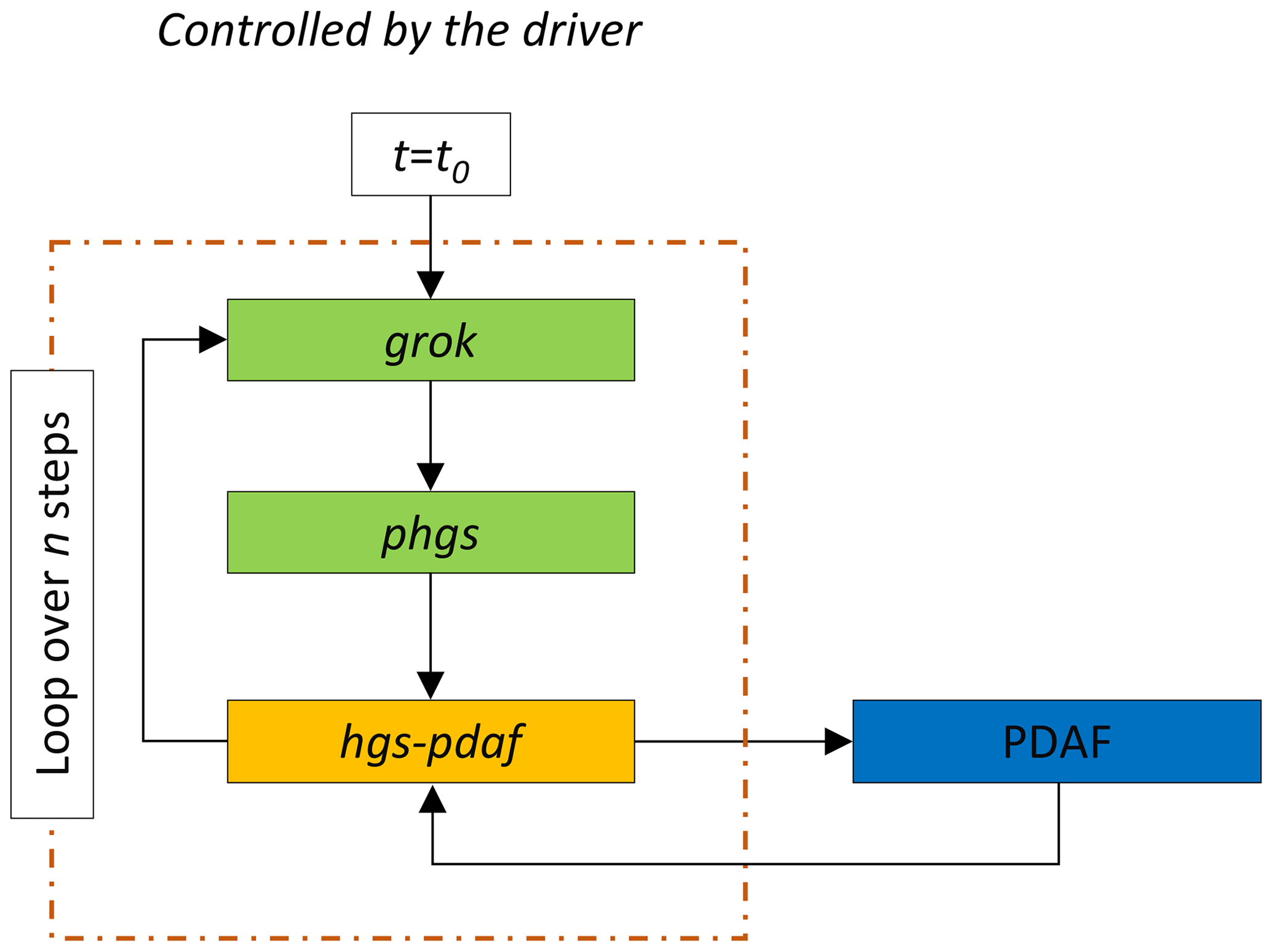
Figure 2 Flowchart of the overall HGS-PDAF workflow. The green blocks are the parts associated with the HGS model, the yellow block is the model bindings that couple HGS to PDAF, and the blue block is the PDAF software itself.

Consider a DA run with HGS-PDAF for an ensemble of m state realisations and a transient model with a total runtime that splits into n time steps of equal interval t_int. Before starting the run, an initial ensemble of m different model realisations needs to be created. The initial ensemble should account for the uncertainty inherent to the natural hydrological system to be simulated. These realisations can be generated in a number of different ways and take into account several different sources of uncertainty, for example, uncertainty in initial conditions, model parameters, boundary conditions and external forcings. Subsequently, the run can be started. At the first time step t=t₀, the process is as follows:

• 1.

  The ensemble of HGS models is initialised/pre-processed in parallel by grok. The model mesh, boundary conditions, parameters and initial conditions are checked and read.

• 2.

  The ensemble of HGS models is run in parallel for t_int by phgs. This is the most computationally demanding step, as it requires running all HGS model realisations forward in time. In the current version of hgs-pdaf, no model run failure management option is implemented, which requires that all model realisations need to successfully completed for continuation of the run.

• 3.

  Now hgs-pdaf is executed. Figure 3 shows the call sequence within hgs-pdaf. The steps are as follows:

  • 3.1

    The parallelisation for PDAF is initialised. The MPI commands are defined for the respective filter.

  • 3.2

    The data assimilation is initialised. The parameter values for PDAF in the configuration files in the Fortran namelist format are read. See Sect. 3.3.2 for a detailed description of these configuration files. Next, the dimension of the state vector is determined. The state variables and parameters from step (2) are read from the output files of HGS. Their values, called “forecast”, are entered into the state vector. This is done for each ensemble state.

  • 3.3

    The ensemble mean and standard deviation of the ensemble of state vectors are written to a netCDF file Output.nc. In addition, if required, the results for each realisation are written to m netCDF files Output_ens_i.nc, where i represents the realisation.

  • 3.4

    The observations are mapped into the state space by the observation operator. PDAF then performs the analysis step of the data assimilation by integrating the observations with the model forecast according to the chosen DA algorithm, e.g. using the EnKF. The ensemble of state vectors is then updated now holding the “analysis”.

  • 3.5

    The “analysis” state information is written into the file Output.nc analogous to Step 3.3. The ensemble of “analysis” state vectors is written into HGS format in parallel for each ensemble member. These files will be used as the initial condition for computing the next time step with HGS.

  • 3.6

    PDAF is finalised which completes the execution of hgs-pdaf for this analysis time step.

Steps (1)–(3) are repeated until $t=t_{\mathrm{int}}\cdot n$. In the current implementation, DA results at every analysis time step are stored in netCDF format, while the original output files of the HGS model at the final step are also retained.

Figure 3 Call sequence of different subroutines within hgs-pdaf.

3.3 Model bindings: hgs-pdaf

To couple HGS with PDAF, a number of routines – known as model bindings – provide PDAF with the information from HGS and subsequently pass information from PDAF back to HGS after DA. Since these model bindings are written in Fortran, the following text uses terminology as it is called in Fortran. The main program is responsible for calling various HGS and DA subroutines sequentially. The subroutines/modules developed are grouped and described as follows.

3.3.1 Initialisation subroutines

These subroutines are designed to initialise the parallelisation, parameterisation and state vector for DA. The MPI execution environment is initialised in init_parallel_pdaf at the very beginning. Initialisation of PDAF is done by init_pdaf. This includes the following parts as shown in Fig. 4:

1. Parameters such as the filter type, localisation and inflation are predefined in init_pdaf. Parameters specified in namelist files are read by read_config_pdaf.

2. The information about the model mesh, such as the total number of nodes and elements in the model, is read in by the HGS_init function.

3. The setup and dimension of the state vector is defined in initialise. It is calculated by the details given in (1) and (2). For example, if the state vector, as per the definition in (1), contains the hydraulic heads (i.e. a hydrological system state, defined for each model node) and K (i.e. a hydraulic parameter, defined for each model element), then the number of nodes for the hydraulic heads is n_nodes, and the number of elements for K is n_elements, which is defined in (2). In this case the dimension of the state vector as calculated by initialise would be $n_{\mathrm{state}}=n_{\mathrm{nodes}}+$ n_elements.

4. Information about the configuration of the DA, as defined by the initialisation subroutines, can be printed out by init_pdaf_info.

5. The values for the nodes that have been set to define the state vector are also read at this point from the ensemble of HGS runs that were run forward in time, i.e. the “forecast”. This is done directly in init_pdaf. Variables included in the state vector can be hydraulic heads, soil water saturation, solute concentrations (modelled system states) and K (model parameter). Notice that we may need to transfer the original values of the model state or parameters, e.g. for K; the log-transformed K is considered in the state vector rather than the K itself used in the HGS model to ensure that K is always positive during the assimilation process.

6. Initialise the DA output netCDF files Output.nc by init_output_pdaf.

Figure 4 Flowchart of the initialisation of data assimilation.

3.3.2 Parameterisation modules

The parameters for HGS and DA are predefined in the initialisation phase. However, for each DA application, users should define them according to their system knowledge and needs. These parameter values are defined in the two namelist files, namelist.pdaf and namelist.hgs, that are provided by the user. The available parameters that can be defined in the namelist files are described in Appendix B. These two namelist files are read by the subroutine read_config_pdaf in the initialisation phase. The parameters used in DA and HGS will then be replaced with the values specified in these namelist files instead of the default values defined in init_pdaf by read_config_pdaf.

3.3.3 Observation modules

For each observation type, a different observation module obs_VAR_pdafomi exists. Here, VAR refers to the name of each type of observation, for now hydraulic heads (HEAD), soil moisture (SAT) and solute concentrations (CONC), but more can be added easily. These different observation modules are independent of each other, allowing for several different types of observations to be modularly combined and assimilated either separately or in a chosen combination. Below, the functioning of the observation modules is described with the example of hydraulic heads.

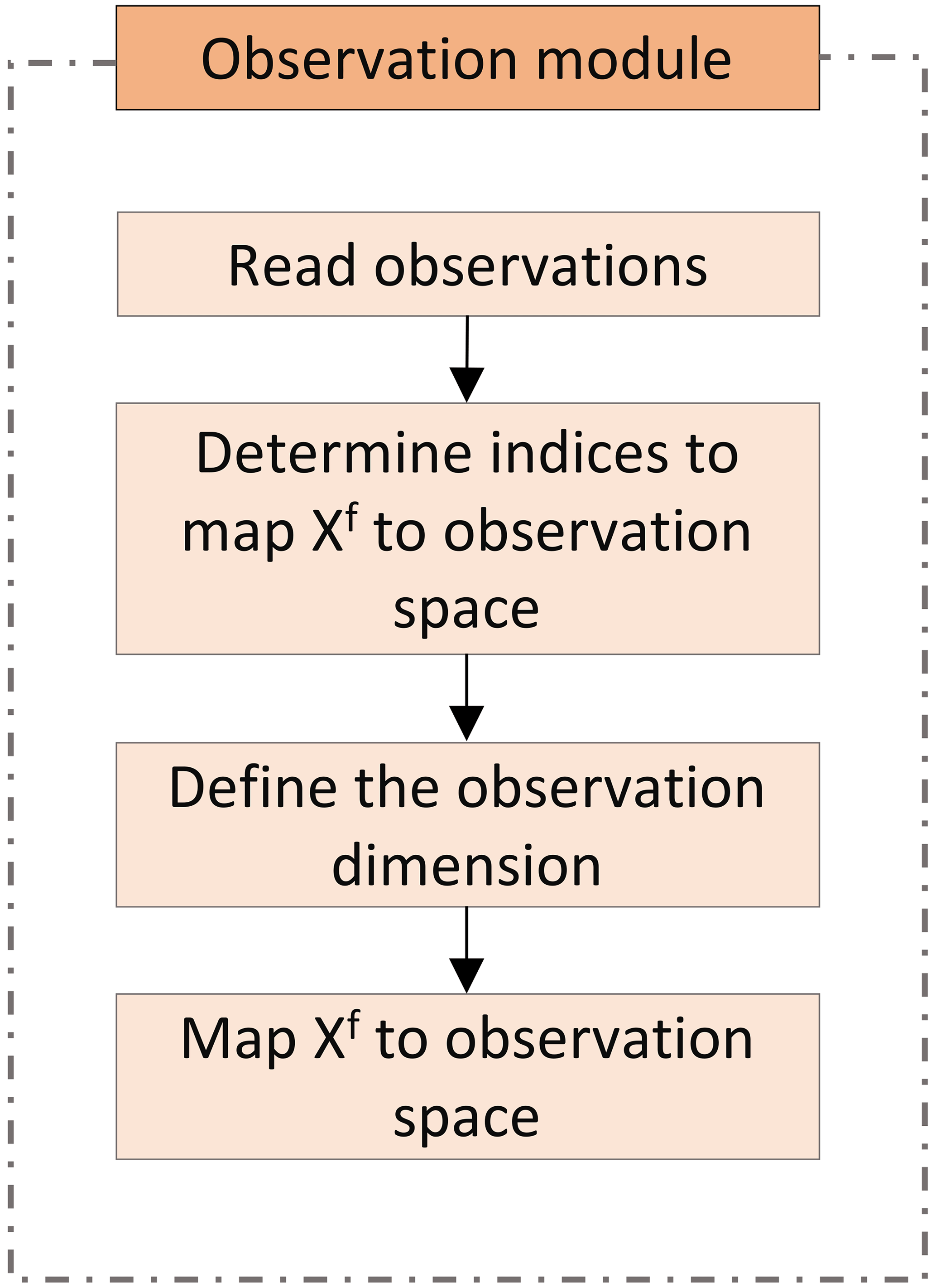
Like every observation module, the obs_HEAD_pdafomi module contains subroutines that initialise the information about the observations (init_dim_obs_HEAD) and apply the observation operator (obs_op_HEAD). Hydraulic head observations are read from the observation input file by init_dim_obs_HEAD. The number of observations at the current time step is then counted, which define the dimension of the observation vector for the observation type, in this case hydraulic head. The observations are checked by excluding the unreasonable values (e.g. by defining a threshold value), and the indices of the observations deemed usable during the current time step are stored. The coordinates, the values and the errors in the respective observations are also stored.

Obs_op_HEAD is the implementation of the observation operator. Thus, it is responsible for the mapping between the state and the observation domains. Various observation operators from PDAF can be selected here by calling the corresponding subroutine PDAFomi_obs_op_X. It is also possible for the user to add their own observation operator here. Figure 5 gives an overview of how the observation module works.

Figure 5 Illustration of the observation module.

The subroutine init_dim_obs_pdafomi is used to combine the different observations. This subroutine provides an interface between PDAF and the different observation modules. init_dim_obs_pdafomi calculates the full dimension of the observation vector by combining all the chosen observation types.

3.3.4 Assimilation subroutine

The subroutine assimilation_pdaf handles the DA analysis step. The DA algorithm is called according to the filter type defined in the namelist.pdaf file. The corresponding filter then updates the variables stored in the state vectors.

3.3.5 Pre- and post-processing subroutines

At each time step, the ensemble mean and standard deviations of the state vector at the prediction and analysis stages are computed by the prepoststep_ens_offline subroutine. By default, all these values are written to the output netCDF file Output.nc. This is done by the subroutine write_netcdf_pdaf in the output_netcdf module which contains various subroutines to write the results of the DA into files. In addition, if the user requires the output of all the individual ensemble members, the subroutine write_netcdf_pdaf_ens can write the results of each ensemble member to separate netCDF files Output_ens_i.nc. Note that these DA output files are different from the output files of the HGS model, which are stored separately in the original format.

When data assimilation is complete for a time step, an important step is to write the updated states (and parameters) back to the original HGS model format so that they can subsequently be used as new initial conditions and parameters for the next simulation time step. This is done by calling output subroutines to write files that are compatible with HGS at the end of the main HGS-PDAF program. The development of these output subroutines is beyond the scope of this paper.

3.4 Scalability of HGS-PDAF

The HGS-PDAF code is parallelised with MPI and uses only CPUs. For the scalability test, we used the illustrative example described in Sect. 4. Different ensemble sizes varying from 2 to 100 members/realisations were tested. Each model was run on one individual core, thus peaking at 100 cores for the case of 100 ensemble members. All the test runs were carried out on JURECA-DC CPUs from the Jülich Supercomputing Centre in Germany. The clock speed per computing node is 2.25 GHz. The individual HGS simulation is not parallelised; i.e. each HGS model is run on one core. Figure 6 shows the scaling behaviour of HGS-PDAF on the JURECA-DC CPUs. The execution time is normalised with the time for an ensemble size of two members. When the ensemble is increased from 2 to 100, the execution time increases by about 50 %.

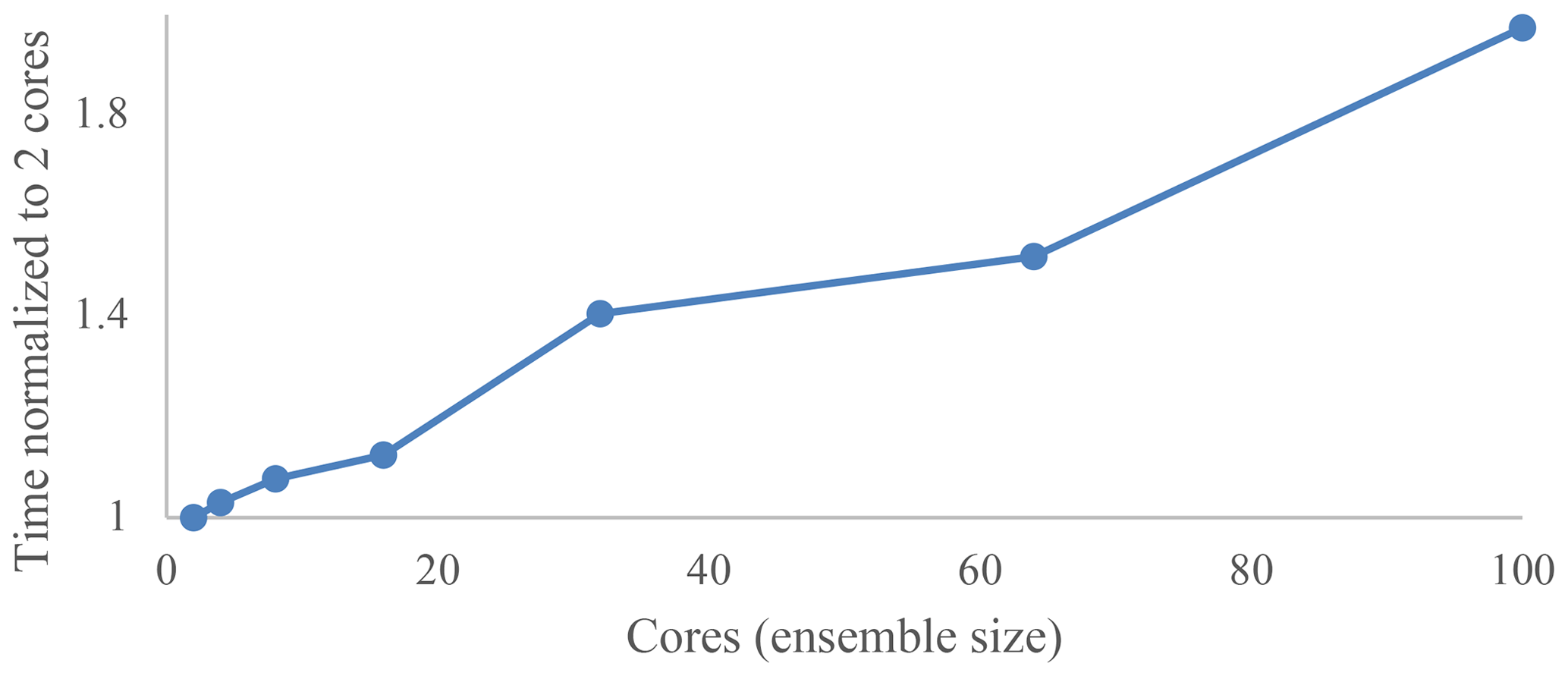
Figure 6 Computing time of HGS-PDAF on JURECA-DC for different ensemble sizes between 2 and 100 normalised by the time for ensemble size two.

4 Illustrative examples of the capabilities of HGS-PDAF

Here, the capabilities of HGS-PDAF are illustrated using a quasi-hypothetical numerical river–aquifer model designed based on a real-world riverbank filtration site in the Swiss pre-Alps which has already served for several studies as a model system for tracer and DA method development (Tang et al., 2018; see Popp et al., 2021; Schilling et al., 2022). The model was thus designed to be representative of an alluvial river–aquifer system where groundwater is pumped for drinking water supply from wells located in the direct vicinity of a river, inducing so-called bank filtration. Such systems are highly suitable for drinking water production owing to the high K and natural filtration capacity of the alluvial sand and gravel materials which make up the riverbed and the aquifer. However, in such systems, the interactions between rivers and the underlying aquifers can be highly dynamic, changing from losing to gaining conditions, and back, within just a few tens of metres, and the heterogeneity of the alluvial sand and gravel material can be very complex, with irregular paleochannels potentially leading to strong preferential flow. Without suitable observations and integrated numerical flow and transport models, understanding and managing such systems becomes a major challenge. Therefore, DA and integrated surface–subsurface hydrological modelling tools, in particular our HGS-PDAF, are of high interest to continuously update and correct model predictions for optimal decision support. This quasi-hypothetical model was chosen to demonstrate the capability of HGS-PDAF to consistently reproduce both system states and parameters even in a highly dynamic and complex hydrological system.

4.1 Basic model setup

The real-world alluvial sand and gravel aquifer system, according to which the illustrative model was designed, is characterised by a distinct paleochannel of well-sorted gravel that exhibits substantially higher hydraulic conductivities compared to the surrounding, unsorted alluvial sand and gravel sediments (Schilling et al., 2022). The slightly abstracted, generalised synthetic version of the real-world site model has been introduced by Delottier et al. (2022b) for the development of environmental gas tracer transport simulations with an ISSHM and efficient data space inversion techniques for complex heterogeneous aquifer systems (Delottier et al., 2023).

Geometrically, the model represents a three-dimensional rectangular domain with dimensions of 500 m × 300 m × 30 m (Fig. 7). A river of 20 m width and 2 m depth is explicitly represented in the model at X=0 m. The horizontal resolution of the finite elements mesh varies between 4 m along the river and riverbanks and 7 m on the alluvial plain. Vertically, the model consists of 14 layers, with thicknesses ranging from 0.5 to 4 m on the alluvial plain and slightly smaller thicknesses underneath the river and riverbanks. In total, the model consists of 112 240 nodes and 204 000 elements. Two riverbank filtration pumping wells, spaced at 100 m and located at a distance of approximately 90 m parallel to the river, extract groundwater from a depth of 14 m. The heterogeneity in K as typically found in such alluvial river–aquifer systems is implemented via a highly conductive paleochannel.

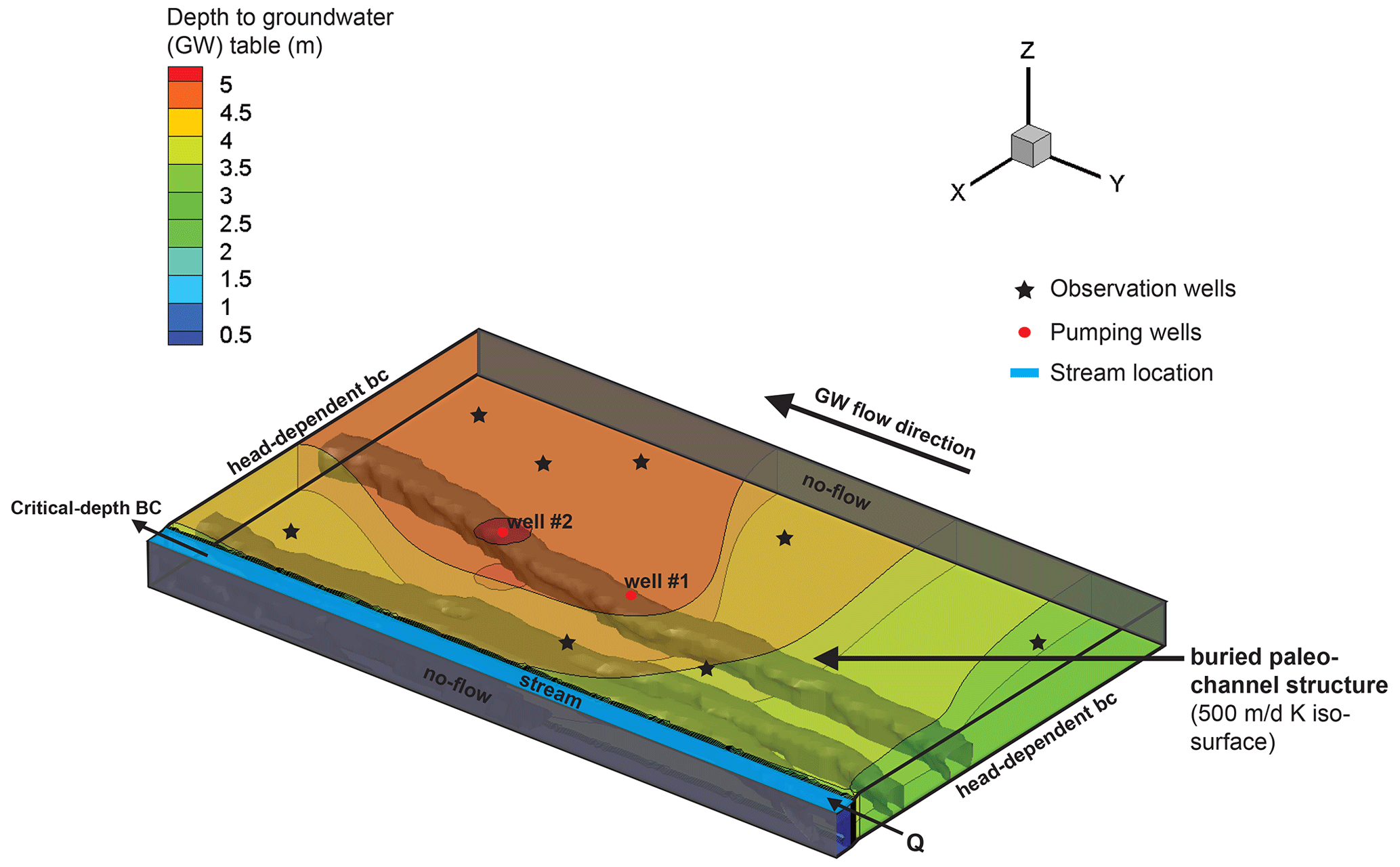
Figure 7 Three-dimensional view of the model domain and model boundary conditions. Contours represent the groundwater table depth below the surface. Locations of eight virtual observation wells are marked as stars. The location of the highly conductive paleochannel is indicated by a 500 m d⁻¹ iso-surface for K.

In the surface domain, constant boundaries are set for the upstream with an inflow rate of 1.71 m³ s⁻¹. A critical depth boundary is set as a boundary condition for the outflow of the stream. In the subsurface domain, a head-dependent Cauchy-type boundary condition was applied to the groundwater flow. At the upstream, a constant hydraulic head of 99.5 m was assumed, while at the downstream, a constant hydraulic head of 93.2 m was considered. The conductance for these boundaries was set to 5.8 m² s⁻¹. The model was forced with transient boundary conditions to reproduce a controlled pumping experiment in which pumps are first running at a constant rate of 400 m³ h⁻¹ for 15 d and are subsequently turned off for 50 d, after which they are again turned back on to a constant rate of 400 m³ h⁻¹ for the remaining 30 d of the experiment (Fig. 8). A coupling length of 0.001 m is used to account for the exchange fluxes between the surface and the subsurface domains. Figure 7 shows a three-dimensional view of the model domain, boundary conditions and paleochannel location, while Fig. 8 shows a schematic of the transient pumping rates employed for the experiment.

Figure 8 Transient pumping rates during the simulation period.

In HGS, time steps are adaptive so that no specific restrictions were applied to maximum time step sizes, with the limitation that the maximum time step size could not be larger than the assimilation time step as defined for PDAF. The initial conditions were obtained for each model realisation individually via a 1-year spin-up run with constant boundary conditions corresponding to the conditions at the beginning of the 95 d pumping experiment.

4.2 Prior ensemble and synthetic observations

In this study, the prior uncertainty of the system is characterised by the observed variance of the initially generated ensemble of hydraulic properties (i.e. the K). A comprehensive description of the generation of the ensemble is described in Delottier et al. (2023). Briefly, the prior ensemble was developed by using a stochastic alluvial feature generator ALLUVSIM (Pyrcz et al., 2009), geared towards the generation of an alluvial sand and gravel aquifer with distinct paleochannel features. To represent the well-sorted paleochannel and the unsorted surrounding sediments, two categorical parameter fields were created and each of these two categories was populated with a spatially uniform K (i.e. producing two types of sediments with homogeneous properties each). In this way, hydraulic conductivities were parameterised on a model element basis, producing a heterogeneous parameter field. During DA, the K value of each of these numerical model elements was adjusted. In addition to these heterogeneous K fields, an ensemble of 100 realisations with different homogeneous K values was also considered for the experiments for comparison purposes. These 100 homogeneous K values were defined as the arithmetic averages of the 100 heterogeneous K fields.

To generate synthetic observations against which the performance of DA could be evaluated, one of the stochastic realisations of the ALLUVSIM simulations was defined as a reference heterogeneous K field or synthetic “truth”. This reference heterogeneous K field is illustrated in Fig. 7. To generate observations for the assimilation experiment, eight locations within the model domain were chosen and daily time series of hydraulic heads and soil water saturation at a depth of 1.5 m were extracted from this reference simulation. These observation time series were subsequently stochastically perturbed by a normally distributed error with a standard deviation of 5 cm for hydraulic heads and 1 % for soil water saturation. The values of the observation errors are determined by our prior knowledge and tuning experiments. Different percentages such as 5 % and 10 % were tested and subsequently defined to provide a more illustrative use case.

4.3 Data assimilation scenarios

To demonstrate the modularity and capability of HGS-PDAF, 20 different DA scenarios that cover combinations between

• single and multivariate assimilations of hydraulic heads and/or soil moisture observations,

• updating either one or a combination of states (i.e. hydraulic heads and/or soil water saturation),

• joint update of one or a combination of states alongside the parameter K, and

• one of two scenarios of prior uncertainty in K (i.e. heterogeneous or homogeneous properties)

were run. As a DA algorithm, the EnKF was chosen. The assimilation interval is 1 d. When hydraulic heads and soil water saturation are updated together, the initial condition for the next prediction cycle is only hydraulic head. In addition, runs without DA (so-called “open-loop” runs) were carried out for both the heterogeneous and the fully homogeneous K scenarios.

Owing to the relatively small size of the simulated system, no localisation was applied. For the heterogeneous K scenarios, when K was updated with DA, a damping factor of less than 1 was applied. For the homogeneous K scenarios, as the assumption of homogeneity already acted as a regularisation for the parameterisation of K, the enforced homogeneity in K during the update always produced a large enough ensemble spread; i.e. the damping factor is equal to 1. Table 1 gives the values of the damping factor used for all DA scenarios.

Table 1 Overview of illustrative DA scenarios. The open-loop scenarios, that is, the scenarios without updating, are labelled “ol”. For all scenarios with updating, the following naming convention applies: the first part of the name identifies the variables that were included in the state vector (i.e. the variables that were updated), while the second part identifies the observations that were assimilated. h, k and s stand for hydraulic head, K and soil water saturation, respectively. Individual damping factors and the conceptualisation of the prior K values are also indicated for each scenario.

For all the scenarios, hgs-pdaf was run on a highly parallelised Linux cluster so that all individual ensembles in the priors were executed in parallel. It took approximately 11 h for hgs-pdaf to complete one single scenario.

4.4 Results and discussion of the illustrative DA experiment

The performance of DA with HGS-PDAF is evaluated by comparing the simulated hydraulic heads and soil water saturation to the synthetically observed hydraulic heads and soil water saturation, respectively. The average relative difference (over the eight observation wells) between the simulated (represented by the ensemble mean) and synthetically observed states are illustrated in Fig. 9. Results are presented for all the scenarios and for the two different prior ensembles (i.e. homogeneous and heterogeneous K fields).

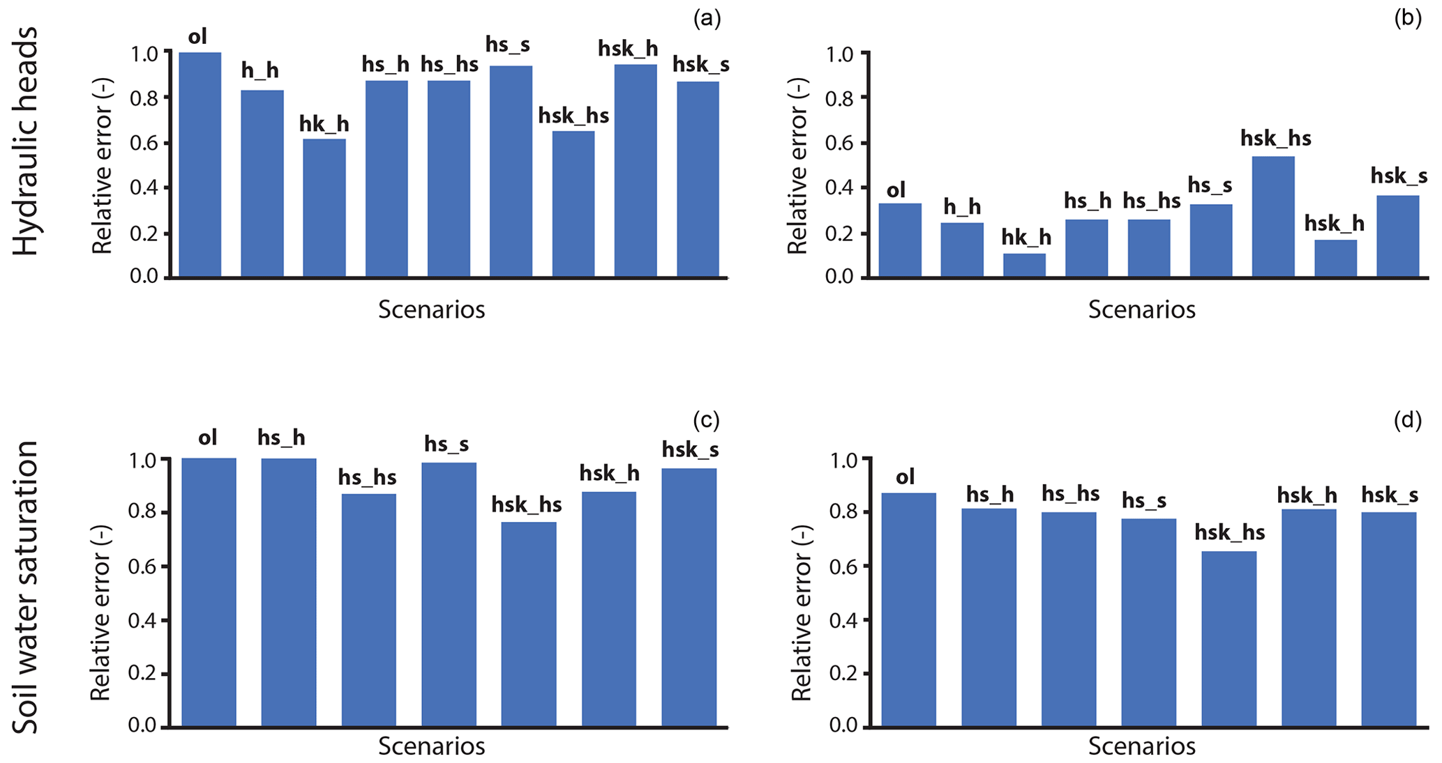
Figure 9 Ensemble mean of the relative differences (averaged for all observation wells) between simulated and observed states (hydraulic heads and soil water saturation) for (a, c) the homogeneous scenarios and (b, d) the heterogeneous scenarios. For the soil water saturation, only scenarios where soil water saturation was updated are shown.

It is remarkably clear from Fig. 9 how DA applied to an ISSHM of a riverbank filtration site (by using HGS-PDAF) is able to reduce the misfit for almost all scenarios and for the two prior ensembles. Overall, the model performance (with respect to both employed observation types) is significantly better when starting from and allowing heterogeneous K-fields to arise, compared to when employing the assumption of homogeneity.

For hydraulic heads, the best performance in reducing the model misfit was obtained when assimilating hydraulic heads and updating both hydraulic heads and K (DA_hk_h). Little to no improvements were gained by assimilating also soil water saturation alongside hydraulic heads. In the heterogeneous case, scenario DA_hk_h performed so well that the averaged ensemble mean model error was reduced to reflect the measurement error (5 cm). On the other hand, scenario DA_hsk_hs, in which hydraulic heads, soil water saturation and K were all updated together based on observations of hydraulic heads and soil water saturation, performed the worst. Even when a low damping factor was used, K values did not improve and turned out highly unrealistic (results not shown). On the other hand, spurious updates of K were not observed in the DA_hsk_hs scenario when run with the homogeneity assumption, as the homogeneity assumption helps to regularise the problem and ensures consistent estimates of homogeneous K fields. The poor performance for updating K in the heterogeneous scenario can likely be attributed to the fact that updating categorical prior parameter fields violates the multi-Gaussian assumption inherent to the ensemble Kalman filter (Evensen et al., 2022). In such cases, other methods such as data space inversion (DSI) or multiple point geostatistics (MPS) should produce better results (Remy et al., 2009; Delottier et al., 2023).

For soil water saturation, the overall model performance was less improved by DA compared to the improvement for the reproduction of hydraulic heads. The largest improvement was achieved when hydraulic heads, saturation and K were updated jointly using both observations of hydraulic heads and soil water saturation (scenario DA_hsk_hs). On the other hand, very little improvement on model performance could be achieved when only observations of soil water saturation were assimilated, irrespective of the combination of states (and parameters) chosen to be updated. This poor performance of using soil water saturation observations for DA of an ISSHM is likely explained by the fact that soil water saturation observations stem from locations relatively far away from the stream and which therefore did not show a strong variation throughout the pumping experiment. In this specific configuration, the information contained in observations of saturation was thus limited and could not match up against the information contained in hydraulic heads, which varied strongly throughout the pumping experiment.

Figure 10 Posterior estimates of K fields with heterogeneous priors for three different scenarios and two individual realisations. The bottom row indicates the probability of occurrence of a paleochannel, calculated by considering a given threshold (i.e. 600 m d⁻¹) above which a buried paleochannel facies is potentially identified.

Concerning reproducing the true K field, as long as the K fields were updated from heterogeneous priors and heterogeneous structures were allowed to arise during updating, a reasonably good overall agreement could already be achieved by only using hydraulic heads (Figs. 9 and 10). This is certainly partly owed to the fact that the initially chosen heterogeneous prior was a priori a good approximation of the synthetic truth, as can be directly seen in the two examples illustrated in Fig. 10 as well as in the relatively good performance of the heterogeneous open-loop run. As such, this illustrative case highlights the importance of choosing as good a prior as possible in such heterogeneous K systems, particularly because paleochannel facies are, as outlined previously, difficult to identify from hydraulic head observations alone. Nevertheless, even though the performance of DA was generally good even for K, the non-multi-Gaussian connectivity of the structures could not be preserved perfectly during DA with HGS-PDAF, as can be seen in Fig. 10. As outlined previously, however, this is an expected outcome of DA with a multi-Gaussian method such as EnKF.

5 Conclusions

We have here introduced a new data assimilation framework for fully integrated surface–subsurface hydrological models by providing a coupling between the ISSHM HGS and the DA software PDAF. This highly modular DA framework allows for the single and multivariate assimilation of several types of observational data, including hydraulic heads, soil water saturations and solute concentrations, as well as an individual or joint update of several model states and parameters, including hydraulic heads, soil water saturation, solute concentrations and hydraulic conductivities. The scalability of HGS-PDAF was evaluated at the Jülich Supercomputing Centre in Germany, and the usability and modularity of HGS-PDAF was illustrated with a synthetic river–aquifer and bank filtration model and the standard ensemble Kalman filter method (one of several DA algorithms provided by PDAF). Compared to existing hydrological data assimilation systems, the advantage of the newly developed HGS-PDAF lies in its consideration of ISSHM; its large selection of different assimilation algorithms as provided by PDAF; its modularity with respect to combining observations, states and parameters to be considered for DA; and the flexibility and ease at which new observations, states and parameters may be added to the already implemented ones. While in the current version of HGS-PDAF only global filters are implemented, the implementation of localised filters is planned for the next iteration.

Appendix A

Table A1 Data assimilation approaches in PDAF and their known application fields.

Appendix B: namelist files

The parameters that need to be defined in the namelist.hgs file are listed in Table B1. These parameters are used for the HGS model.

The parameters that can be defined in the namelist.pdaf file are listed in Table B2. These parameters are used for data assimilation. If the values of these parameters are not specified in namelist.pdaf, default values are used. A detailed description of these parameters can be found from the PDAF website (http://pdaf.awi.de, last access: 19 April 2024).

Table B1 Parameters defined in namelist.hgs.

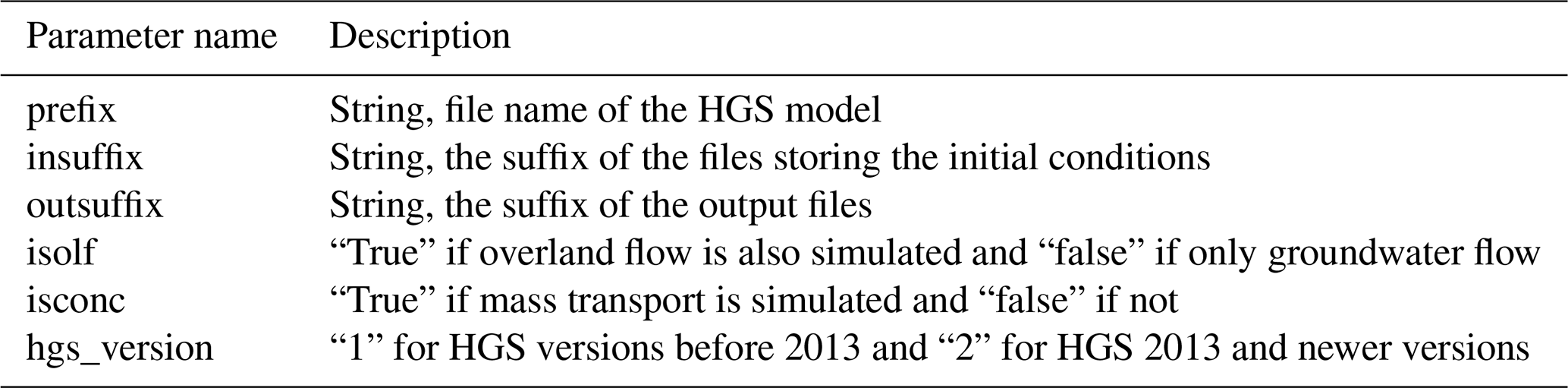
Table B2 Parameters defined in namelist.pdaf.

^∗ “True” if yes and “false” if no.