Assessing acetone for the GISS ModelE2.1 Earth system model

Acetone is an abundant volatile organic compound (VOC) in the atmosphere, with important influences on ozone and oxidation capacity. Direct sources include chemical production from other VOCs and anthropogenic emissions, terrestrial vegetation, biomass-burning emissions, and ocean production. Sinks include chemical loss, deposition onto the land surface, and ocean uptake. Acetone also has a lifetime that is long enough to allow transport and reactions with other compounds remote from its sources. The NASA Goddard Institute for Space Studies (GISS) Earth system model ModelE2.1 simulates a variety of Earth system interactions. Previously, acetone had a very simplistic representation in the ModelE chemical scheme. This study assesses a more sophisticated acetone scheme in which acetone is a full 3-dimensional tracer with explicit sources, sinks, and atmospheric transport. We first evaluate the new global acetone budget in the context of past literature. Estimated source and sink fluxes fall within the range of previous models, although total atmospheric burden and lifetime are at the lower end of the published literature. Acetone's new representation in ModelE2.1 also results in more realistic spatial and vertical distributions, which we compare against previous models and field observations. The seasonality of acetone-related processes was also studied in conjunction with field measurements, and these comparisons show promising agreement but also shortcomings at high-emission urban locations, where the model's resolution is too coarse to capture the true behavior. Finally, we conduct a variety of sensitivity studies that explore the influence of key parameters on the acetone budget and its global distribution. An impactful finding is that the production of acetone from precursor hydrocarbon oxidation has strong leverage on the overall chemical source, indicating the importance of accurate molar yields. Overall, our implementation is one that corroborates with previous studies and marks a significant improvement in the development of the acetone tracer in GISS ModelE2.1.

1 Introduction

Acetone (C₃H₆O) is an abundant oxygenated volatile organic compound (VOC) that has important connections to ozone and the atmosphere's self-cleansing oxidation capacity (Read et al., 2012). Acetone's dynamic presence in Earth's atmosphere can be described through sources, sinks, and mechanisms of transport. Extensive literature has discussed the nature of these sources and sinks, and some are more well constrained than others.

Primary sources of acetone in the atmosphere include anthropogenic sources, terrestrial vegetation, and biomass-burning emissions. Past literature has found the fluxes of these sources to range between 1–2, 30–45, and 2.5–4.5 Tg yr⁻¹, respectively (Beale et al., 2013; Brewer et al., 2017; Elias et al., 2011; Fischer et al., 2012; Folberth et al., 2006; Jacob et al., 2002; Singh et al., 2000; Wang et al., 2020). Chemical production from other VOCs with three or more carbon atoms, each with their own molar yield, is another source of acetone in the atmosphere (Brewer et al., 2017; Fischbeck et al., 2017; Hu et al., 2013; Jacob et al., 2002; Singh et al., 2000; Weimer et al., 2017).

Sinks of acetone include wet and dry deposition as well as chemical loss. Wet deposition occurs within and below clouds due to the solubility of acetone and depends on its Henry's law coefficient (Benkelberg et al., 1995). Dry deposition occurs on the land surface. Chemical loss of acetone forms radicals through photolysis. Past literature has estimated the acetone sinks to be 10 %–30 % dry deposition and 40 %–85 % chemical loss (Arnold et al., 2005; Elias et al., 2011; Fischer et al., 2012; Khan et al., 2015; Singh et al., 1994). The estimated fluxes are 10–16 and 45–60 Tg yr⁻¹ for total deposition and chemical loss, respectively (Arnold et al., 2005; Brewer et al., 2017; Dufour et al., 2016; Elias et al., 2011; Fischer et al., 2012; Jacob et al., 2002; Khan et al., 2015; Marandino et al., 2005; Singh et al., 2000; Wang et al., 2020).

The ocean surface is a bidirectional flux that provides both a source and a sink for acetone. Ocean surface conditions such as wind speed, sea surface temperature, and seawater concentration of acetone can influence the direction and magnitude of ocean–acetone exchange (Wang et al., 2020). Previous literature estimated an oceanic source flux of 25–50 Tg yr⁻¹ and an oceanic uptake flux of 35–60 Tg yr⁻¹. However, there is little consensus in the literature on whether the ocean serves as a net source or sink of acetone, with some studies indicating a net oceanic source (Beale et al., 2013; Jacob et al., 2002; Wang et al., 2020) and other studies indicating a net oceanic sink (Brewer et al., 2017; Elias et al., 2011; Fischer et al., 2012; Wang et al., 2020).

In addition to a global annual mean atmospheric budget, previous studies have reported the seasonality of acetone-related processes. Past studies have compared monthly estimates of acetone mixing ratios to field measurements at European sites from Solberg et al. (1996) (Arnold et al., 2005; Elias et al., 2011; Jacob et al., 2002). Comparisons with these European sites have emphasized the seasonal variability of acetone emissions, as nearly all sites portray a summer maximum and winter minimum of acetone abundance. Vegetation emissions from June to September, along with chemical sources, make an especially strong contribution to this seasonality. The winter minimum of acetone is aided by an ocean sink at coastal sites (Jacob et al., 2002).

Other studies have described the spatial distributions and seasonal dependence of ocean fluxes of acetone (Fischer et al., 2012; Wang et al., 2020). A model by Fischer et al. (2012) proposed a net ocean sink of 2 Tg yr⁻¹ and characterized the ocean uptake of acetone as being strongest in northern latitudes year-round and in the high southern latitudes during the winter. An oceanic acetone source was dominant in the tropical regions, with exceptions occurring off the western coasts of Central America and Central Africa (Fischer et al., 2012). A model by Wang et al. (2020) that varied surface seawater acetone concentration through a machine-learning approach also proposed a net ocean sink year-round. This net sink was strongest in December–February and weakest in March–May.

The vertical distribution of acetone at the surface and in the troposphere between the seasons of May–October and November–April has been modeled (Fischer et al., 2012). Acetone concentrations are generally higher at lower altitudes due to the proximity to surface emissions. Surface-level acetone has been measured over a variety of terrestrial and oceanic sites around the world (de Gouw et al., 2004; Dolgorouky et al., 2012; Galbally et al., 2007; Guérette et al., 2019; Hu et al., 2013; Huang et al., 2020; Langford et al., 2010; Lewis et al., 2005; Li et al., 2019; Read et al., 2012; Schade and Goldstein, 2006; Singh et al., 2003; Solberg et al., 1996; Warneke and de Gouw, 2001; Yoshino et al., 2012; Yuan et al., 2013), and, in some cases, these measurements were taken over a variety of months to provide a sense of seasonality (Dolgorouky et al., 2012; Hu et al., 2013; Read et al., 2012; Schade and Goldstein, 2006; Solberg et al., 1996). Additionally, vertical distributions of acetone have been measured through NASA's Atmospheric Tomography Mission (ATom) campaigns (Thompson et al., 2022). The ATom-1, ATom-2, ATom-3, and ATom-4 campaigns took place during July–August 2016, January–February 2017, September–October 2017, and April–May 2018, respectively. Each campaign provided mixing ratios for a variety of VOCs in profiles from the marine boundary layer up to the upper troposphere and lower stratosphere (Apel et al., 2021).

The NASA Goddard Institute for Space Studies (GISS) ModelE2.1 Earth system model (Kelley et al., 2020) has the capability of simulating a variety of Earth system interactions, is used to both interpret and predict past and future climate, and routinely participates in the Climate Model Intercomparison Project (CMIP) and Intergovernmental Panel for Climate Change (IPCC) reports. Here, we used and enhanced this model by adding acetone as an independent chemical tracer (Kelley et al., 2020). Previously, acetone had a very simplistic representation in the model's chemical scheme (Shindell et al., 2003); acetone's spatial variation was parameterized based on the difference between the model's zonal mean distribution of isoprene and that tracer's three-dimensional distribution. Acetone's lifetime is long enough to be transported such that it is remote from sources, but it is not long enough to become uniformly mixed, and therefore its simulated distribution should benefit from a more realistic implementation. We developed a greatly improved acetone tracer scheme by making prognostic calculations of the 3-dimensional distribution of acetone as a function of time. We evaluated its atmospheric burden and lifetime as well as source and sink fluxes (anthropogenic emissions, vegetation emissions, biomass burning, deposition, and ocean and chemistry fluxes) against other models and its concentration against field measurements. This work aims to provide a holistic assessment of the abundance of acetone in the atmosphere.

2 Methodology

Here, we implement acetone in GISS ModelE2.1 based on the literature rather than developing a new parameterization. Our “baseline” simulation is a climatological mean with year 2000 conditions, chosen to be relatively modern without precluding a comparison with models in older literature. The 1996–2004 mean of prescribed emissions from Hoesly et al. (2018) was used along with the 1996–2005 mean sea surface temperature and sea ice cover, as described in Kelley et al. (2020). Acetone simulations use full chemistry and not archived OH fields. An additional simulation, “Nudged_ATom”, was conducted for a more direct comparison with ATom field measurements. This simulation employed nudged winds from MERRA2 (Gelaro et al., 2017), ocean surface conditions from PCMDI-AMIP 1.1.4 for 2016–2017 (Taylor et al., 2000) and from the Hadley Centre's HadISST1.1 for 2018 (Met Office, Hadley Centre, 2006), and trace gas and aerosol emissions that changed over time during 2016–2018.

2.1 Sources

2.1.1 Anthropogenic emissions

Anthropogenic emissions were prescribed using the 1996–2004 averages of the Community Emissions Data System (CEDS) emissions from Hoesly et al. (2018), as prepared for the GISS contributions to the Coupled Model Intercomparison Project Phase 6 (CMIP6) (Kelley et al., 2020). These include sources from agriculture, the energy sector, the industrial sector, residential/commercial/other, international shipping, solvent production and application, the transportation sector, and waste. In line with past studies, we base acetone emissions on those of ketones. VOC23-ketone emissions from Hoesly et al. (2018) were scaled down by the ratio of acetone's molecular weight to the average ketone molecular weight (58.08 g mol⁻¹ $/$ 75.3 g mol⁻¹). Maintaining the resulting spatial and temporal pattern of emissions, the magnitudes were then tuned to be close to that of Fischer et al. (2012), resulting in a total of about 1 Tg yr⁻¹. This resulted in roughly 36.5 % of the CEDS VOC23 ketones being used as acetone emissions. Lacking an accurate way to obtain aircraft acetone emissions from the bulk VOCs available in the emission inventory, we have neglected that sector in the simulations.

2.1.2 Terrestrial vegetation emissions

Emissions from land vegetation were derived from the Model Emissions of Gases and Aerosols from Nature (MEGAN), version 2.1 (Guenther et al., 2012), a new contribution to ModelE. Emission response algorithms in the MEGAN2.1 model are derived from input leaf area indices, solar radiation, temperature, moisture, CO₂ concentrations, plant functional types, and the plant species composition (Guenther et al., 2012). The vegetation acetone emissions in the baseline simulation in GISS ModelE2.1 were calculated to equal 36.1 Tg yr⁻¹.

2.1.3 Biomass-burning emissions

Acetone emissions were prescribed from a 1996–2004 average of the NMVOC-C₃H₆O species from version 2.1 of the biomass-burning dataset of van Marle et al. (2017), used by CMIP6. The acetone mass flux from biomass burning in the baseline simulation was 1.59 Tg yr⁻¹.

Figure 1 shows the biomass-burning emission rate chosen for this study and how it lies within the range of substantial interannual variation. During the 20-year period shown, emissions averaged 1.46 Tg yr⁻¹ with a standard deviation of 0.402, and a spike in the earlier years of emissions to over 2.75 Tg yr⁻¹ is also observed (Fig. 1). On top of any differences across emission inventories, the years considered when reporting emissions may be the reason for disagreements between models, e.g., 2.40–2.80 Tg yr⁻¹ from the 2006 GFED-v2 emission inventory in Elias et al. (2011) and Fischer et al. (2012) compared to 3.22 Tg yr⁻¹ from 1997–2001 in Folberth et al. (2006).

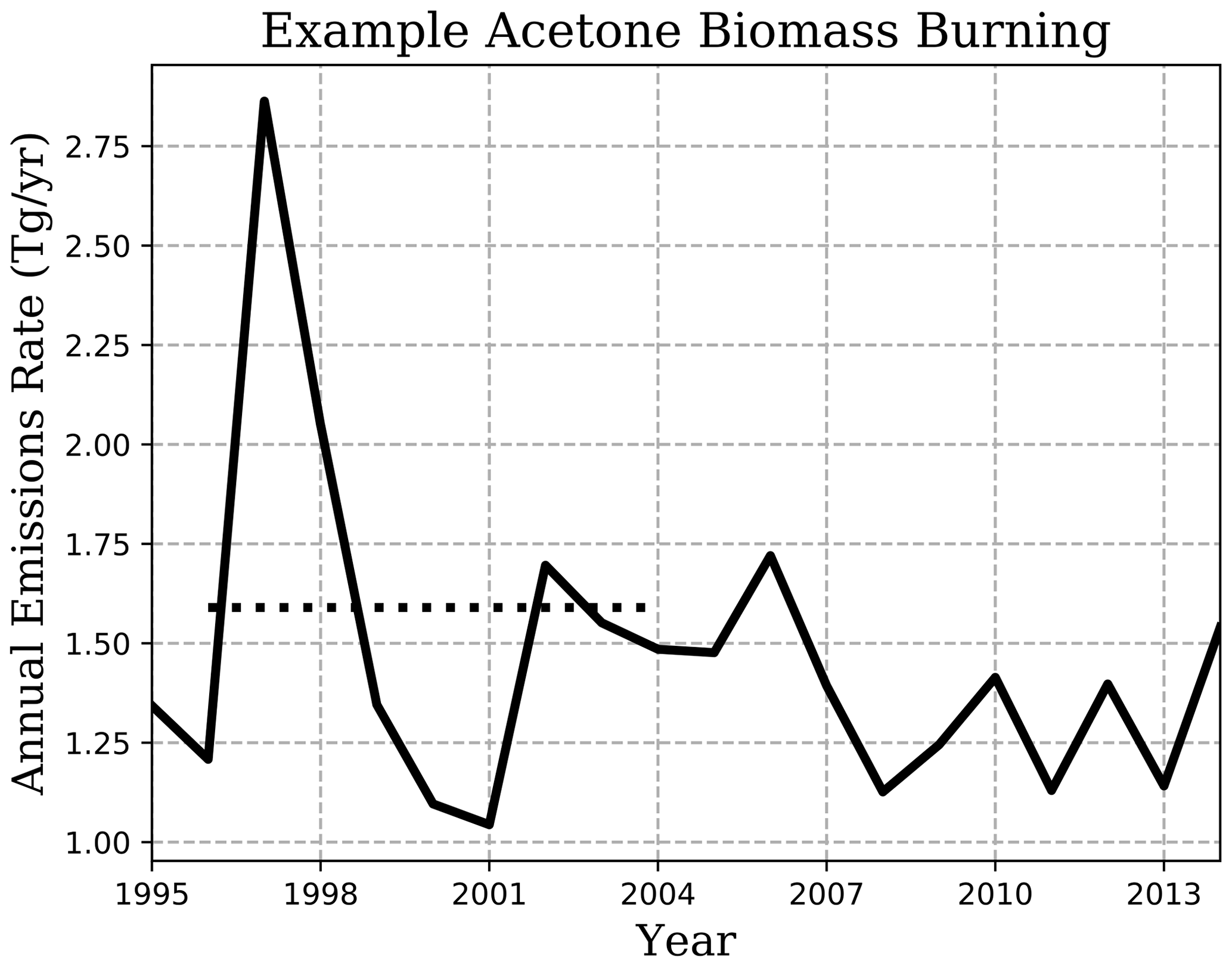
Figure 1 Illustration of the interannual variation in NMVOC-C₃H₆O biomass-burning emissions of van Marle et al. (2017) (solid line), used as acetone emissions in our simulation. Climatological-emissions simulations use the 1996–2004 mean (dotted line), though emissions vary by month.

2.2 Sinks

2.2.1 Deposition

Both dry and wet deposition of acetone were included in the model, although dry deposition was, on average, 91 % of the total deposition. The wet deposition scheme is given by Koch et al. (1999). Acetone and other species are transported within and below clouds, and soluble gases are deposited depending on the conditions of the grid box they are in and a Henry's law coefficient (Shindell et al., 2001). The Henry's law coefficient for acetone used in GISS ModelE2.1 is 27 mol L⁻¹ atm⁻¹, with a Henry temperature dependence of acetone of 5300 J mol⁻¹ (Benkelberg et al., 1995; Zhou and Mopper, 1990). The dry deposition scheme uses resistance-in-series calculations, global seasonal vegetation data (Chin et al., 1996; Shindell et al., 2001; Wesely and Hicks, 1977), and a reactivity factor of f₀=0.1. This resulted in an acetone deposition rate in the baseline simulation of 22.2 Tg yr⁻¹.

2.3 Chemistry

The GISS ModelE2.1 baseline simulation estimates a net chemistry flux of −20.6 Tg yr⁻¹. The components can be broken up into sources and sinks as follows.

2.3.1 Chemical sources

The baseline simulation estimates chemical production to be 33.3 Tg yr⁻¹. The acetone chemical scheme includes two production reactions:

$$\begin{array}{}\text{(R1)}& {\displaystyle }\mathrm{Paraffin}+\mathrm{OH}\to \mathrm{0.35}\mathrm{Acetone}.\text{(R2)}& {\displaystyle }\mathrm{Terpenes}+\mathit{\{}\mathrm{OH},{\mathrm{O}}_{\mathrm{3}}\mathit{\}}\to \mathrm{0.12}\mathrm{Acetone}.\end{array}$$

In the first reaction, acetone is produced by paraffin, a proxy tracer for paraffinic (saturated) carbon, and OH (Reaction R1). The molar yield of acetone from paraffin was found to be a strong leverage on the overall chemical source (see Sect. 3.5). A rate coefficient of $\mathrm{8.1}\times {\mathrm{10}}^{-\mathrm{13}}$ cm³ molec.⁻¹ s⁻¹ was used (Shindell et al., 2003). Previous literature has suggested an acetone yield on a molecular scale of 0.72 (Fischbeck et al., 2017; Jacob et al., 2002; Weimer et al., 2017). Initial tests using a yield of 0.72 resulted in an overestimated chemistry source, leading us to re-evaluate this yield for the specific mixture of VOCs represented in GISS ModelE2.1.

Our model's anthropogenic emissions of paraffin are based on an aggregation of selected VOC groups. Based on year 2019 emissions from the O'Rourke et al. (2021) dataset, we emit paraffin that is about 11 % propane, 22 % butane, and 21 % pentane by mole. Multiplying these by each VOC's acetone molar yield (0.73, 0.95, and 0.63, respectively), we estimate that 42 % of the paraffin from anthropogenic sources becomes acetone in our model. Paraffin biomass-burning emissions estimated from year 2020 of the SSP3_70 emissions (Riahi et al., 2017; Fujimori et al., 2017) contain mole fractions of propane and higher alkanes of 9 % and 23 %, respectively. When multiplied by acetone molar yields of 0.73 and 0.79, respectively, these suggest that about 25 % of the paraffin from biomass-burning sources becomes acetone in our model. The molar yields used in these calculations were derived based on suggestions from the literature (Fischbeck et al., 2017; Jacob et al., 2002; Weimer et al., 2017). Refer to the “Chemical sources” section of the Supplement for a more detailed breakdown. Overall, the average of the 42 % of the anthropogenic paraffin and the 25 % of the biomass-burning paraffin was used to conclude that approximately 35 % of the paraffin from emissions becomes acetone, leading to our refinement of the molar yield in Reaction (R1) to 0.35.

Additionally, reactions between terpenes and {OH,O₃} were implemented with an acetone yield of 0.12 (Hu et al., 2013; Jacob et al., 2002) (Reaction R2). The rates for these reactions are $\mathrm{2.51}\times {\mathrm{10}}^{-\mathrm{11}}$ e${}^{(\mathrm{444}/T)}$ cm³ molec.⁻¹ s⁻¹ for the OH reaction and $\mathrm{1.40}\times {\mathrm{10}}^{-\mathrm{14}}$ e${}^{(-\mathrm{732}/T)}$ cm³ molec.⁻¹ s⁻¹ for the O₃ reaction, and these coefficients are enhanced from the standard α-pinene one to consider the reactivity variability across monoterpenes and higher terpenes (Tsigaridis and Kanakidou, 2003).

2.3.2 Chemical sinks

The chemical sink of acetone in the baseline simulation is estimated to be 53.8 Tg yr⁻¹. The sinks of acetone include oxidation by OH and Cl radicals and photolysis:

$$\begin{array}{}\text{(R3)}& {\displaystyle }\begin{array}{rl}& \mathrm{Acetone}+\mathrm{OH}\to {\mathrm{H}}_{\mathrm{2}}\mathrm{O}+{\mathrm{CH}}_{\mathrm{3}}\mathrm{C}\left(\mathrm{O}\right){\mathrm{CH}}_{\mathrm{2}}\\ & \left(\mathrm{assumed}\mathrm{to}\mathrm{decompose}\mathrm{to}\mathrm{HCHO}\right).\end{array}\text{(R4)}& {\displaystyle }\begin{array}{rl}& \mathrm{Acetone}+\mathrm{Cl}\to \mathrm{HCl}+{\mathrm{CH}}_{\mathrm{3}}\mathrm{C}\left(\mathrm{O}\right){\mathrm{CH}}_{\mathrm{2}}\\ & \left(\mathrm{assumed}\mathrm{to}\mathrm{decompose}\mathrm{to}\mathrm{HCHO}\right).\end{array}\text{(R5)}& {\displaystyle }\mathrm{Acetone}+\mathrm{h}\mathit{\nu }\to {\mathrm{CH}}_{\mathrm{3}}\mathrm{CO}+{\mathrm{CH}}_{\mathrm{3}}.\text{(R6)}& {\displaystyle }\mathrm{Acetone}+\mathrm{h}\mathit{\nu }\to {\mathrm{CH}}_{\mathrm{3}}+{\mathrm{CH}}_{\mathrm{3}}+\mathrm{CO}.\end{array}$$

The first and second acetone destruction reactions above have rates of $\mathrm{1.33}\times {\mathrm{10}}^{-\mathrm{13}}+\mathrm{3.82}\times {\mathrm{10}}^{-\mathrm{11}}$ e${}^{(-\mathrm{2000}/T)}$ and $\mathrm{7.70}\times {\mathrm{10}}^{-\mathrm{11}}$ e${}^{(-\mathrm{1000}/T)}$ cm³ molec.⁻¹ s⁻¹, respectively (Sander et al., 2011) (Reactions R3, R4). Previously, acetone photolysis (which only affected the production of radicals and not acetone itself) did not utilize the model's photolysis scheme; it was parameterized solely as a function of orbital geometry and atmospheric pressure. In the model updates, photolysis now consists of two separate reactions where acetone forms either CH₃CO + CH₃ radicals or two CH₃ radicals and CO (Reactions R5, R6). The spectroscopic data used for acetone photolysis are from JPL 2010 (Sander et al., 2011) and are mapped onto the wavelength intervals of Fast-J version 6.8d (Neu et al., 2007). The photolysis cross section for Reaction (R5) is pressure dependent while that of Reaction (R6) is temperature dependent, leading to variation in yields with altitude and location. For example, in a standard atmosphere, the ratio of the yield of CO to CH₃CO decreases from 0.28 at the surface to 0.18 at 4 km altitude.

2.4 Ocean

Bidirectional fluxes of acetone are calculated over the ocean based on the “two-phase” model of molecular gas exchange at the air–sea interface of Liss and Slater (1974) as described in Johnson (2010). The fluxes are a function of simulated surface temperature and near-surface wind speed but are independent of salinity. The Henry's law constants and temperature dependence of the solubility for acetone are from Sander (2023). The source from ocean water and sink from the atmosphere are calculated assuming a constant concentration of acetone in water (of 15 nM), the lower-boundary-layer atmospheric concentration, and the total transfer velocity (a combination of water-side and air-side transfer velocities). The constant concentration of 15 nM follows the implementation by Fischer et al. (2012) in the GEOS-CHEM model. They looked at observations and did not find a strong reasoning to make the concentration vary seasonally or spatially. The GISS ModelE2.1 baseline simulation calculates the ocean to be a net source of acetone, producing 3.94 Tg yr⁻¹.

2.5 Sensitivity studies

Sensitivity studies were conducted to determine the influence of key parameters on the acetone budget and its global distribution (summarized in Table 1). Specifically, we were interested in seeing the sensitivity of simulated acetone to artificial perturbations of given parameters. Sensitivity studies for chemistry modify the production of acetone. The Chem_Cl0 and Chem_Terp0 simulations provide no formation of acetone from chlorine or terpenes, respectively. The importance of paraffin is explored by halving its yield of acetone to 17.5 % in the Chem_Par0.5 simulation and by doubling its yield of acetone to 70 % in the Chem_Par2.0 simulation. As vegetation was the most prominent source of acetone, the Veg_0.7 simulation investigates a reduction in this source by decreasing the MEGAN production of acetone by 30 %. The Ocn_2.0 simulation aims to explore the impact of the oceanic acetone concentration by doubling it from 15 to 30 nM globally. The Dep_f₀0 simulation tests a drop in the reactivity factor for dry deposition from 0.1 to 0. Finally, given the high interannual variability of biomass-burning emissions, the BB_2.0 simulation explores the impact of doubling those emissions.

Table 1 Sensitivity studies conducted to observe the leverage that a specific parameter had on the model. The names of the simulations and the parameters they target and descriptions of the simulations are included.

3 Results and model evaluation

3.1 Global acetone budget and burden

A global acetone budget table was compiled to place our estimates in context with past global modeling studies (Table 2) (Arnold et al., 2005; Beale et al., 2013; Brewer et al., 2017; Dufour et al., 2016; Elias et al., 2011; Fischer et al., 2012; Folberth et al., 2006; Guenther et al., 2012; Jacob et al., 2002; Khan et al., 2015; Marandino et al., 2005; Singh et al., 2000, 2004; Wang et al., 2020). The values of the individual fluxes in our model (those from global deposition, biomass burning, anthropogenic emissions, and vegetation emissions; ocean net, source, and sink fluxes; and chemistry net, source, and sink fluxes) were mentioned previously.

Table 2 Global acetone budget table comparing the burden, flux, and lifetime estimates for acetone from the baseline model to those from 13 previous studies.

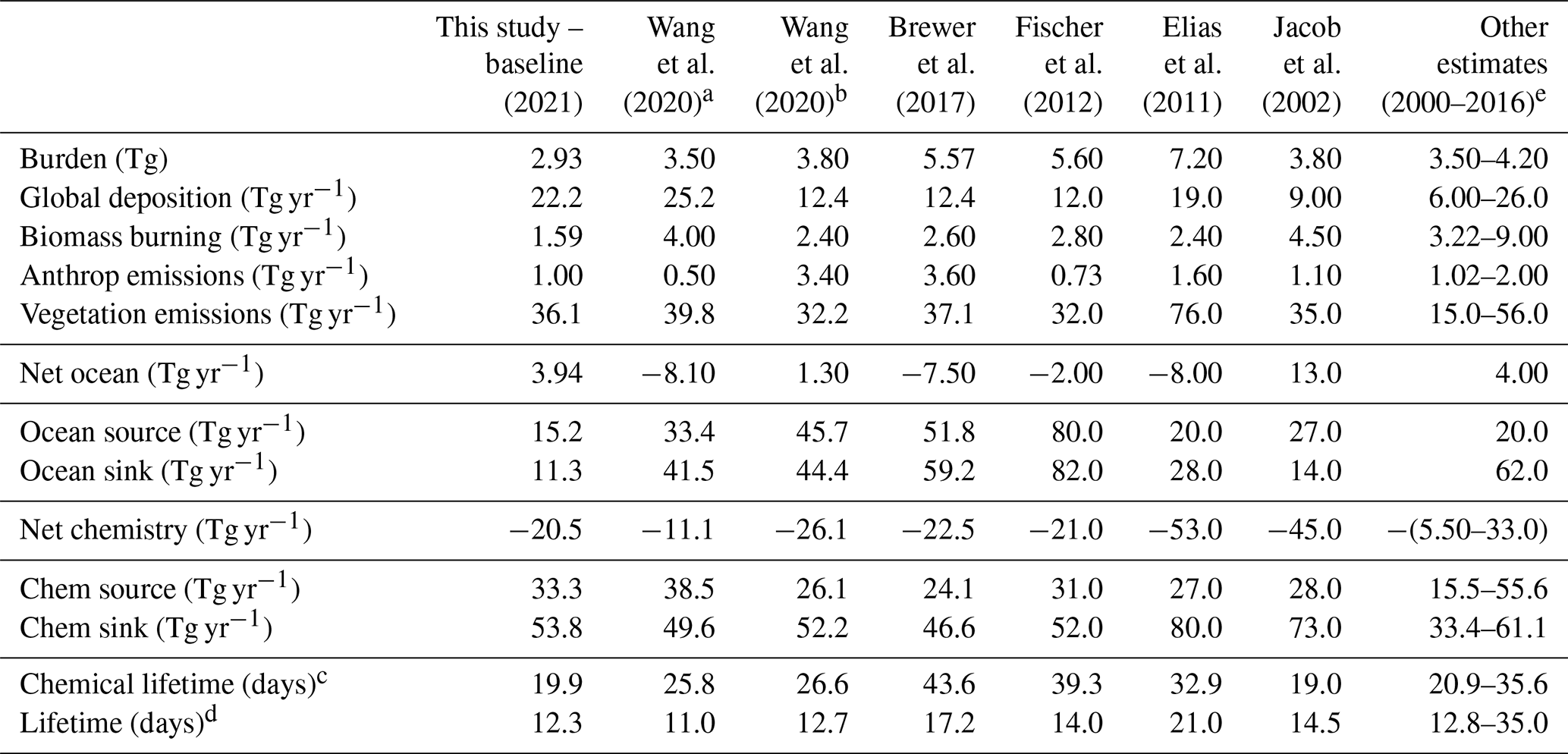
^a CAM-Chem model (Wang et al., 2020). ^b GEOS-Chem model (Wang et al., 2020). ^c Chemical lifetime = burden / chemical sink. ^d Total atmospheric lifetime = burden / total sink. ^e Singh et al. (2000, 2004), Arnold et al. (2005), Folberth et al. (2006), Marandino et al. (2006), Guenther et al. (2012), Beale et al. (2013), Khan et al. (2015), Dufour et al. (2016).

The atmospheric burden describes the total amount of acetone that is in the atmosphere. The GISS ModelE2.1 baseline simulation estimates the burden to be 2.93 Tg. Additionally, the chemical lifetime and atmospheric lifetime can be derived from the burden. The chemical lifetime of acetone is calculated as the burden divided by the chemical sink, whereas the total lifetime is the burden divided by all sinks. The chemical and total atmospheric lifetimes for the baseline simulation are calculated to be 19.9 and 12.3 d, respectively. These values are also placed in the context of previous literature in Table 2.

The GISS ModelE2.1 baseline acetone budget is further compared to previous model studies in Fig. 2. The calculated fluxes in the baseline simulation that are less than 1 standard deviation away from the literature mean include the anthropogenic and vegetation emissions, the net ocean and net chemistry fluxes, and chemical production and chemical destruction (Fig. S1 in the Supplement). The biomass burning in GISS ModelE2.1 appears to be an outlier when compared against nine previous model studies, but this can be attributed to the high interannual variation of emissions (as discussed in Sect. 2.1.3). The value for acetone deposition is at the high (more negative) end in GISS ModelE2.1 relative to 11 previous studies. This might be partially attributed to differences in deposition parameterization across models, as explored by our sensitivity study on dry deposition (presented in Sect. 3.5.2). The values for oceanic acetone sources and losses are smaller (in absolute values) than the mean from seven previous model studies. Nevertheless, the net ocean flux matches the literature well. Lastly, the total atmospheric burden and lifetime calculated by GISS ModelE2.1 are lower than in the previous papers, an expected consequence of the higher removal by deposition. The chemical lifetime is also calculated to be at the low end of published literature.

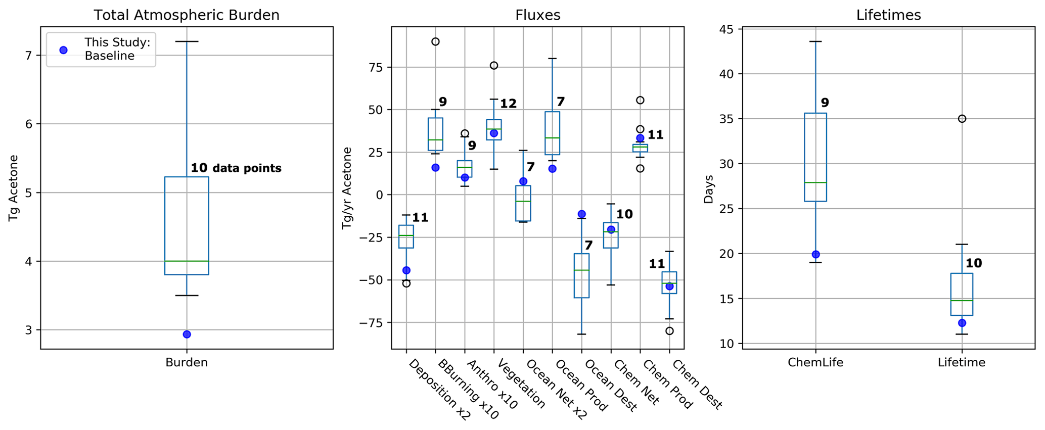
Figure 2 Total atmospheric burden, fluxes, and lifetimes of acetone from the literature values presented in Table 2 (shown as boxes and whiskers, with outliers shown as open circles) and the values from GISS ModelE2.1 (shown as solid blue circles). The number of models used to create each box and whisker plot is labeled. Note that the deposition and ocean net fluxes were multiplied by 2 and that the biomass-burning and anthropogenic emissions were multiplied by 10 for better visualization of the distribution.

3.2 Spatial distribution of acetone

The global distribution of acetone at the surface is given in Fig. 3. It is evident that acetone mixing ratios are largest over the continents, where anthropogenic, vegetation, and other terrestrial sources are located. Over the ocean, acetone mixing ratios are highest downwind of Central America and Central Africa. A comparison of the GISS ModelE2.1 results against 26 prior field measurements shows great agreement overall, with a root mean squared error of 0.3494 and an R² value of 0.8306. To put these results into the context of model evaluation, a similar comparison to field measurements was done for the model's previous acetone scheme. The prior parameterization was designed as a rough representation of acetone oxidized from isoprene in the upper troposphere, without regard for realism near the surface, and this is evident from the comparison with surface observations: a root mean squared error and R² value of 1.3620 and 0.0413, respectively. The improvement of the new acetone tracer model in GISS ModelE2.1 is evident from these statistics.

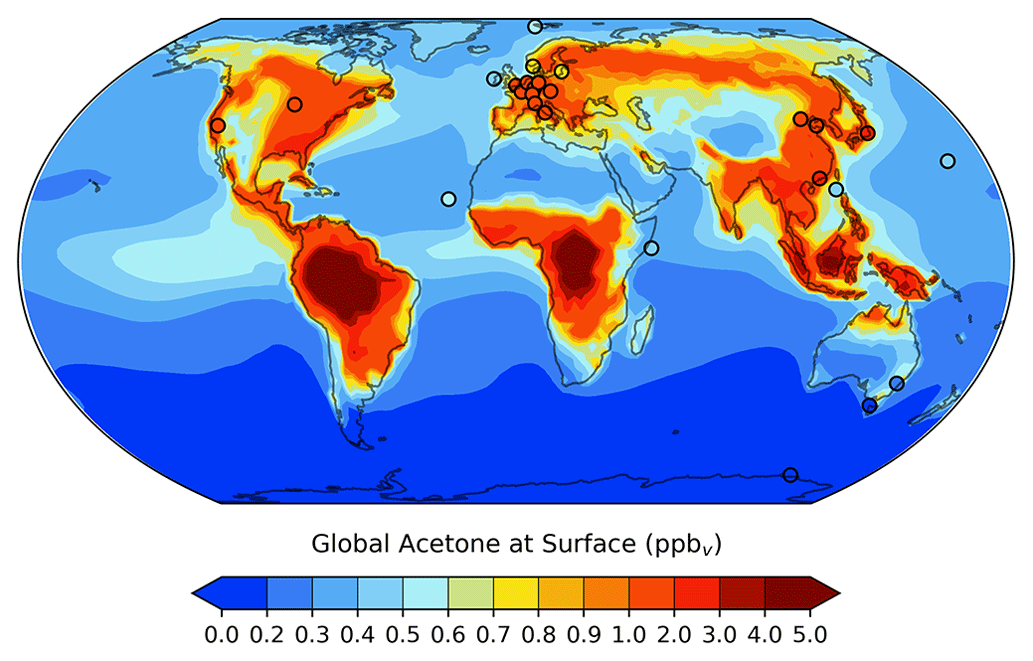
Figure 3 Spatial distribution of annual mean acetone at the surface for the GISS ModelE2.1 baseline simulation. Filled circles represent data from 26 field measurements (de Gouw et al., 2004; Dolgorouky et al., 2012; Galbally et al., 2007; Guérette et al., 2019; Hu et al., 2013; Huang et al., 2020; Langford et al., 2010; Lewis et al., 2005; Li et al., 2019; Read et al., 2012; Schade and Goldstein, 2006; Singh et al., 2003; Solberg et al., 1996; Warneke and de Gouw, 2001; Yoshino et al., 2012; Yuan et al., 2013). The root mean squared error and the R² value between the baseline acetone estimations and the field measurements are 0.3494 and 0.8306, respectively. A nonlinear color bar is used to better differentiate the details in the map.

A breakdown of the bidirectional fluxes of acetone indicates that its chemical production is concentrated over the continents, while chemical destruction primarily occurs over the oceans (Fig. 4). Hotspots of production over the continents include the Southeastern United States and central South America, East and Northern Asia, and Central Africa. Chemical sinks over the oceans are stronger in the tropics than in the high southern or northern latitudes. Annually, there is a net flux of about −20.46 Tg yr⁻¹. Observing the chemical flux across all four seasons, the net loss appears unaffected, while the net source changes more significantly, following the seasonality of precursor compounds like isoprene and terpenes (Fig. 4). Chemical production is strongest in the months of June, July, and August, primarily in North America and Northern Asia. Production is weakest in the months of December, January, and February, with almost all production in North America and Northern Asia lost. Still, a net negative flux is present for all four seasons (Fig. 4).

Figure 4 Net acetone chemistry fluxes (column integrated) in the baseline simulation for December–February (a), March–May (b), June–August (c), and September–November (d), with red indicating a net source and blue indicating a net sink. Nonlinear color bars are used to better differentiate the details in the map. The weighted global mean of the net chemistry fluxes is shown in a box to the lower right of each panel.

The oceanic acetone sources and sinks are unevenly distributed across latitudes (Fig. 5). Oceanic uptake of acetone is mostly concentrated in the northern rather than the southern oceans, while the oceanic acetone source is strongest in the tropics and decreases at higher latitudes in both hemispheres. Combining these two unidirectional fluxes results in the ocean serving as a sink in the northern high latitudes and a source in the tropical latitudes and to be near neutral in the high southern latitudes (Fig. 5). This finding corroborates very well with findings from Fischer et al. (2012) and Wang et al. (2020). Additionally, oceanic bidirectional fluxes of acetone present trends over the four seasons (Fig. S2). Overall, every season has a positive global mean net flux. However, production becomes strongest in the months of December through May and weakest in the months of June through November. Off the coast of western South America, the ocean appears to be a net sink of acetone, even though this latitude band is generally a source of acetone (Figs. 5, S2). This is especially evident in the months of June to August and September to November. As the model simulates this location as having high levels of acetone at the surface (Fig. 3), we believe the acetone in the air is driving the ocean to be a sink there.

Figure 5 Annual mean oceanic acetone uptake (a), oceanic acetone production (b), and net bidirectional flux (c) in the baseline simulation, with red indicating a net source and blue indicating a net sink. Nonlinear color bars are used to better differentiate the details in the map. The corresponding weighted global mean of the ocean fluxes is shown in a box to the lower right of each panel.

3.3 Vertical distribution of acetone

The vertical distribution of acetone varies by latitude, with near-surface air mixing ratios being higher in the tropics and in the northern mid-latitudes (Fig. 6). Acetone levels in the atmosphere decrease with height, a direct result of sinks dominating the sources. Prior to the implementation of an acetone tracer in GISS ModelE2.1, when acetone was derived from the zonal mean of isoprene, the vertical distribution looked very different. Acetone was only concentrated around the tropics and did not extend nearly as high into the troposphere. The complexity of Fig. 6 supports the new acetone tracer scheme as a significant improvement to GISS ModelE.

Figure 6 Vertical distribution of acetone air mixing ratios across latitudes in the GISS ModelE2.1 baseline simulation.

Another modeled vertical distribution of acetone, including a differentiation between two long seasons, is explored in Fig. 7. In general, it was found that acetone mixing ratios are higher in the months of May–October than in November–April, and that this relationship is stronger in the lower atmosphere (0–2 km) than the upper atmosphere (6–10 km). This finding corroborated well with a similar analysis done by Fischer et al. (2012).

Figure 7 Baseline-simulation acetone mixing ratios in the atmosphere at approximately 6–10 km (a, b), 2–6 km (c, d), and 0–2 km (e, f) for the months of May–October (a, c, e) and November–April (b, d, f). The average mixing ratios over these broad altitude layers are weighted by the air mass in the model layers they contain. The slices and colors used match those used in Fig. 1 of Fischer et al. (2012).

Additionally, GISS ModelE2.1 was compared to four ATom campaigns (Thompson et al., 2022) of acetone field measurements in the atmosphere (Apel et al., 2021). For this comparison, we averaged the flight data to the model grid and then compared the resulting mean against the monthly mean fields of the model output. Contrary to other chemical species measured during ATom that vary significantly in space and time, acetone has a rather long lifetime, and the data are collected, for the most part, very far from its sources. This, combined with the fact that prescribed emissions in GISS ModelE2.1 vary by month, not by day or even by hour, makes such a comparison appropriate. Meteorology can, however, affect long-range transport significantly, so we performed a nudged simulation (called Nudged_ATom) towards the MERRA2 reanalysis (Gelaro et al., 2017) to capture this effect more accurately. We also used emissions and greenhouse gas concentrations from the years of the ATom campaigns, varying by year, rather than the climatological means used in the baseline simulation. Both the Nudged_ATom and baseline simulations are plotted in the ATom comparisons presented here (Fig. 8).

Figure 8 Comparison between the GISS ModelE2.1 simulations (baseline in purple and Nudged_ATom in blue) and the ATom-2 field measurements (January–February 2017). Individual data points are shown with dark gray symbols, and their average values are shown in black, with error bars representing the 1-sigma range of the averages. The root mean square error (RMSE) of each simulation is noted at the top right of each panel.

There are very few notable differences between the nudged and climatological simulations. An example is the tropical Atlantic Ocean, where during ATom-2 (Fig. 8), the nudged simulation calculates higher acetone concentrations, but without any gain of skill. Both model simulations miss the upper tropospheric peak that is found in the measurements, likely indicating a missing long-range transported plume. There is a similar result for ATom-3 (Fig. S4) for the southern Atlantic Ocean mid-latitudes, where the nudged simulation is higher. Contrary to the ATom-2 case, both simulations for the ATom-3 case calculate an upper-tropospheric maximum, which is not found in the measurements. The tropical and southern mid-latitude Atlantic Ocean regions are both downwind of African biomass-burning zones during ATom-2 and ATom-3, respectively, hinting at an incorrect primary and/or secondary source of acetone related to biomass burning and subsequent long-range transport. Other than those few cases, for the most part, the two simulations are indistinguishable, indicating that our conclusions upon comparing climatological simulations to ATom should be robust (Figs. 8, S3–S5). This is important to remember in Sect. 3.5.3, where we perform sensitivity analyses that use climatological simulations and compare against all four ATom campaigns.

3.4 Seasonality of acetone

Most European sites presented in Fig. 3 have monthly resolved measurements that can be used to analyze the seasonal behavior of acetone in the model (Figs. 9, S6) (Solberg et al., 1996). These sites differ with respect to their geographic locations and their proximity to anthropogenic sources. Zeppelin, Birkenes, Rucava, and Mace Head are all coastal sites, while Waldhof, Košetice, Donon, Ispra, and Montelibretti are inland sites. Regarding anthropogenic sources, Zeppelin is the most remote location and Birkenes and Rucava each have small sources. Mace Head is a site affected by the marine boundary layer, and Waldhof, Košetice, and Donon are sites with small local anthropogenic sources that are generally located in higher-emission regions. Montelibretti and (particularly) Ispra are subject to the highest anthropogenic sources. The measurements taken at Ispra show an opposite seasonality to what is expected, and previous studies have considered this anomalous (Jacob et al., 2002).

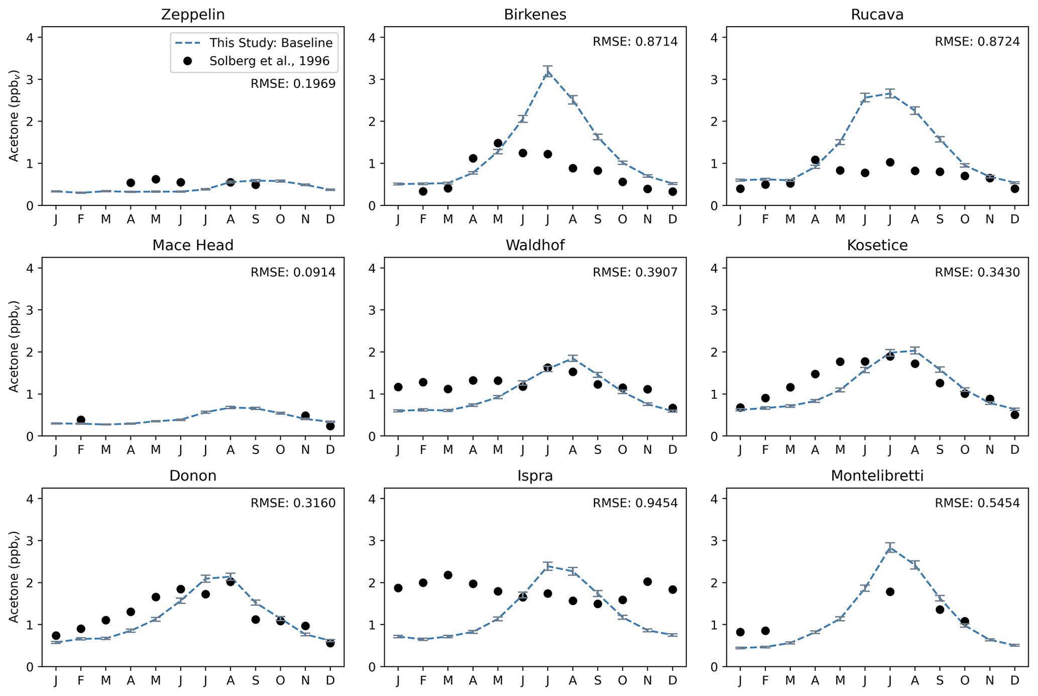
Figure 9 Acetone over 12 months at nine European sites, similar to that of Jacob et al. (2002). The modeled estimates of acetone at the surface from the baseline simulation are shown as dashed blue lines, and the gray error bars represent the 1-sigma range of the modeled concentrations in the climatological mean of 5 years. Field measurements from Solberg et al. (1996) are shown as solid black dots. The root mean squared error between the baseline simulation and field measurements is shown at the top right of each panel.

GISS ModelE2.1 matches the seasonality of the measurements especially well in Zeppelin, Mace Head, Waldhof, Košetice, and Donon; the average root mean square error between the baseline model and the measurements at these five sites are 0.27. The baseline model overestimates the measurements in Birkenes and Rucava (RMSE = 0.87 for both), even though these two sites have low anthropogenic sources. This overestimation has been attributed to the vegetation source, which has a distinct seasonality and is much stronger than any other source there. Interestingly, in Montelibretti, the model's overestimation of vegetation but underestimation of local emissions results in a decent estimation of the sources there (RMSE = 0.55) (Fig. 9).

As mentioned previously, an analysis of the distribution of the regional sources and sinks at the nine European sites shows that, except for Zeppelin and Mace Head, all studied European sites have vegetation as the dominant source that strongly contributes to the simulated seasonality of concentrations (Fig. S7). Vegetation sources peak in the summer months and are lower in the winter. Deposition is a major sink of acetone and is comparable in magnitude with the vegetation source. Ocean uptake of acetone follows a weak seasonal cycle, being stronger in the summer months. Relatively speaking, the other fluxes (anthropogenic emissions, biomass burning, and ocean production) do not exhibit much seasonality at these locations (Fig. S7).

We also compared GISS ModelE2.1's surface acetone at observation sites with less temporal coverage (Fig. S8). In general, GISS ModelE2.1 matches the field measurements well. This is especially true for the non-summer seasons in Rosemount and Berkeley (USA) and the summer peaks in Utrecht (Netherlands) and Mainz (Germany). The model seems to overestimate acetone around Australia, as shown by comparisons with Cape Grim and Wollongong, while it underestimates emissions in large cities like Shenzhen and Beijing (China), London (UK), and Paris (France) (Fig. S8).

3.5 Sensitivity studies

The sensitivity simulations presented here have been described in Sect. 2.5 and in Table 1. We grouped them into two categories: those directly related to chemical sources and sinks and those related to terrestrial and oceanic acetone fluxes. Overall, the sensitivity studies that presented the largest changes to total atmospheric burden included Chem_Terp0, Chem_Par0.5, Chem_Par2.0, Veg_0.7, Ocn_2.0, and Dep_f₀0 (i.e., all but Chem_Cl0 and BB_2.0) (Figs. S9–S14).

3.5.1 Chemistry

Chemistry sensitivity tests that modified the production of acetone were analyzed with respect to the budget and global distribution of acetone. In the Chem_Cl0 simulation, where no acetone oxidation by the chlorine radical occurs, the overall global acetone budget does not change. However, in some places like Rucava, Ispra, Montelibretti, and Shenzhen, the shape of the acetone concentration profile over the year changes slightly (Figs. 10, S15).

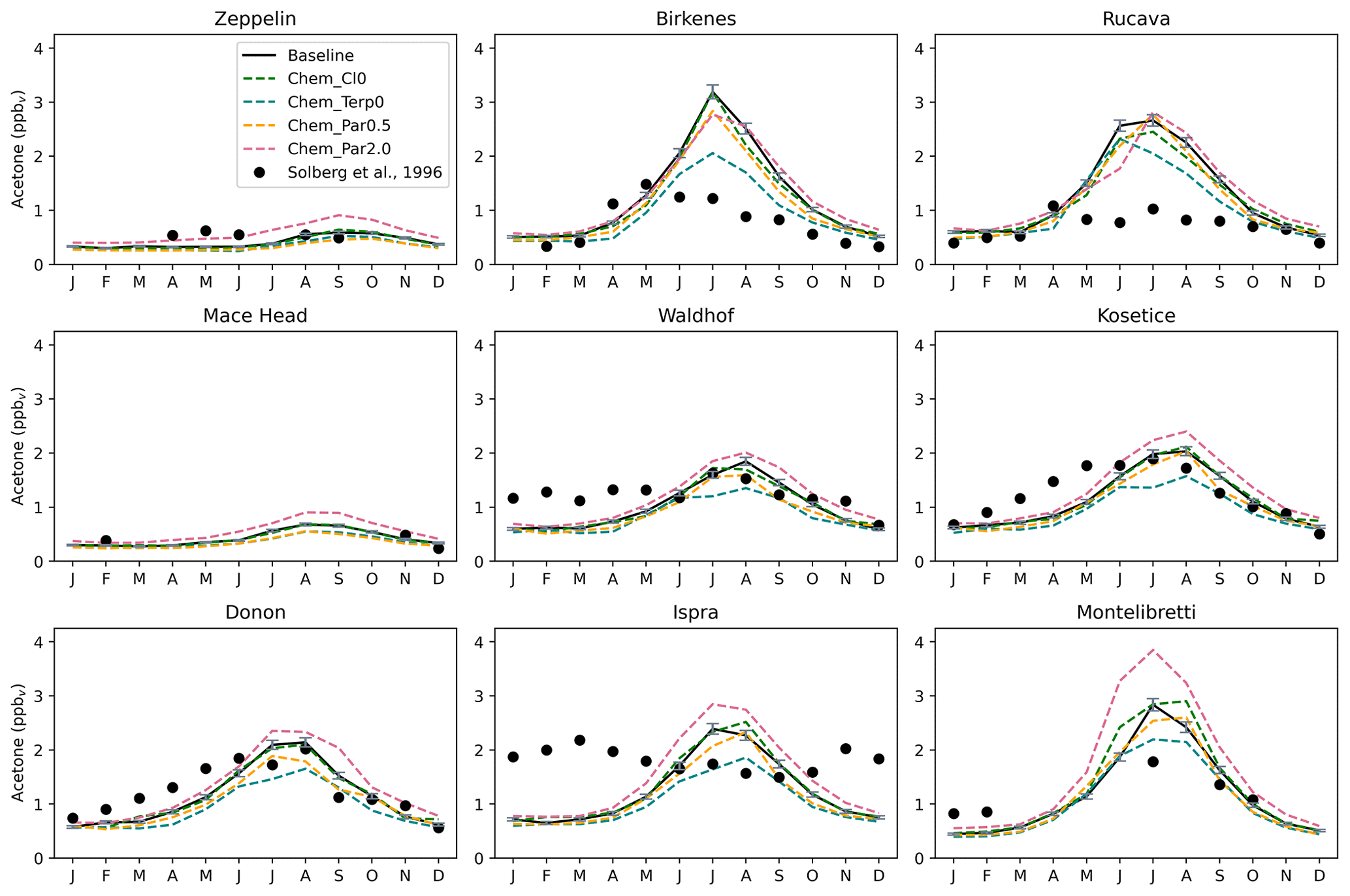
Figure 10 Similar to Fig. 9, but with the chemistry sensitivity studies added. The modeled estimates of acetone at the surface from the baseline simulation are shown as solid black lines, and the sensitivity studies shown here are as follows: removing the acetone + chlorine reaction (dashed green lines), removing the production of acetone from terpenes (dashed blue lines), halving the yield of acetone from paraffin (dashed orange lines), and doubling the yield of acetone from paraffin (dashed pink lines). Field measurements from Solberg et al. (1996) are shown as solid black dots.

The Chem_Terp0 simulation that removes the production of acetone from terpenes decreases the summer peak of acetone by as much as 35.5 % in Birkenes, 25.5 % in Mainz, and 25.3 % in Berkeley (Figs. 10, S15). Other sites, like Montelibretti, Ispra, and Paris, have their summer peak decreased by 22.6 %, 22.2 %, and 19.0 %, respectively (Figs. 10, S15). Coastal and remote areas like Zeppelin, Mace Head, and Dumont d'Urville, Antarctica, are not impacted by the removal of terpenes (Figs. 10, S15).

There seems to be some nonlinearities with the relationship between acetone abundance and its yield from paraffin, as the results from the Chem_Par2.0 and Chem_Par0.5 simulation reveal that doubling the yield has a stronger impact than halving it. For instance, in Montelibretti, doubling the yield from paraffin increases the summer peak by 35.7 %, while halving the yield decreases the summer peak by only 8.3 % (Fig. 10). A similar relationship is also observed at the sites of Ispra (a 19.1 % increase upon doubling the yield from paraffin; a 2.5 % decrease upon halving the yield from paraffin) and Berkeley (a 12.7 % increase upon doubling the yield from paraffin; a 2.5 % decrease upon halving the yield from paraffin) (Figs. 10, S15). Overall, we explored chemistry sensitivities that would tend to push acetone in both directions, and the baseline simulation falls between these tests, which we have identified as important uncertainties.

The spatial distribution differences between the chemistry sensitivity studies and the baseline simulation show some interesting patterns (Fig. S16). Removing the production of acetone from terpene oxidation from the Chem_Terp0 simulation decreased acetone over the continents, especially over tropical and boreal forests, where terpenes are emitted. This change also increased acetone concentrations over the oceans due to chemical composition changes downwind that result from the change in terpene oxidation products (Fig. S16, top left). Halving the production of acetone from paraffin oxidation in the Chem_Par0.5 simulation only decreased acetone concentrations over the continents, while doubling it in the Chem_Par2.0 simulation increased acetone concentrations over the continents and strengthened acetone destruction over the tropical oceans (top right and bottom middle in Fig. S16, respectively). Setting the acetone + chlorine reaction rate to 0 in the Chem_Cl0 simulation resulted in negligible changes across the globe (anomalies of <0.4 ng m⁻² s⁻¹).

3.5.2 Terrestrial and oceanic fluxes

Terrestrial and oceanic flux sensitivities were analyzed at the same sites. The vegetation flux sensitivity, Veg_0.7, reduced acetone production from MEGAN by 30 %. This change decreased the summer peak of acetone at nearly every location studied, but most notably by 32.6 % in Birkenes, 22.9 % in Rucava, and 22.2 % in Rosemount (Figs. S17, S18).

In the oceanic flux sensitivity simulation, Ocn_2.0, the concentration of acetone in the water was doubled from 15 to 30 nM. The results of this simulation varied with geographic location. For instance, in Birkenes, doubling the oceanic concentration reduced the overall acetone by 13.9 %, while in Montelibretti, it was increased by 16.1 % (Fig. S17). Even though Birkenes is more of a coastal city than Montelibretti, this result may simply be a temperature effect: Birkenes is at 58° N, while Montelibretti is at 42° N, and a warmer ocean may produce more acetone. Overall, in most places, doubling the oceanic acetone concentration did not change the atmospheric acetone by much throughout the year (Figs. S17, S18).

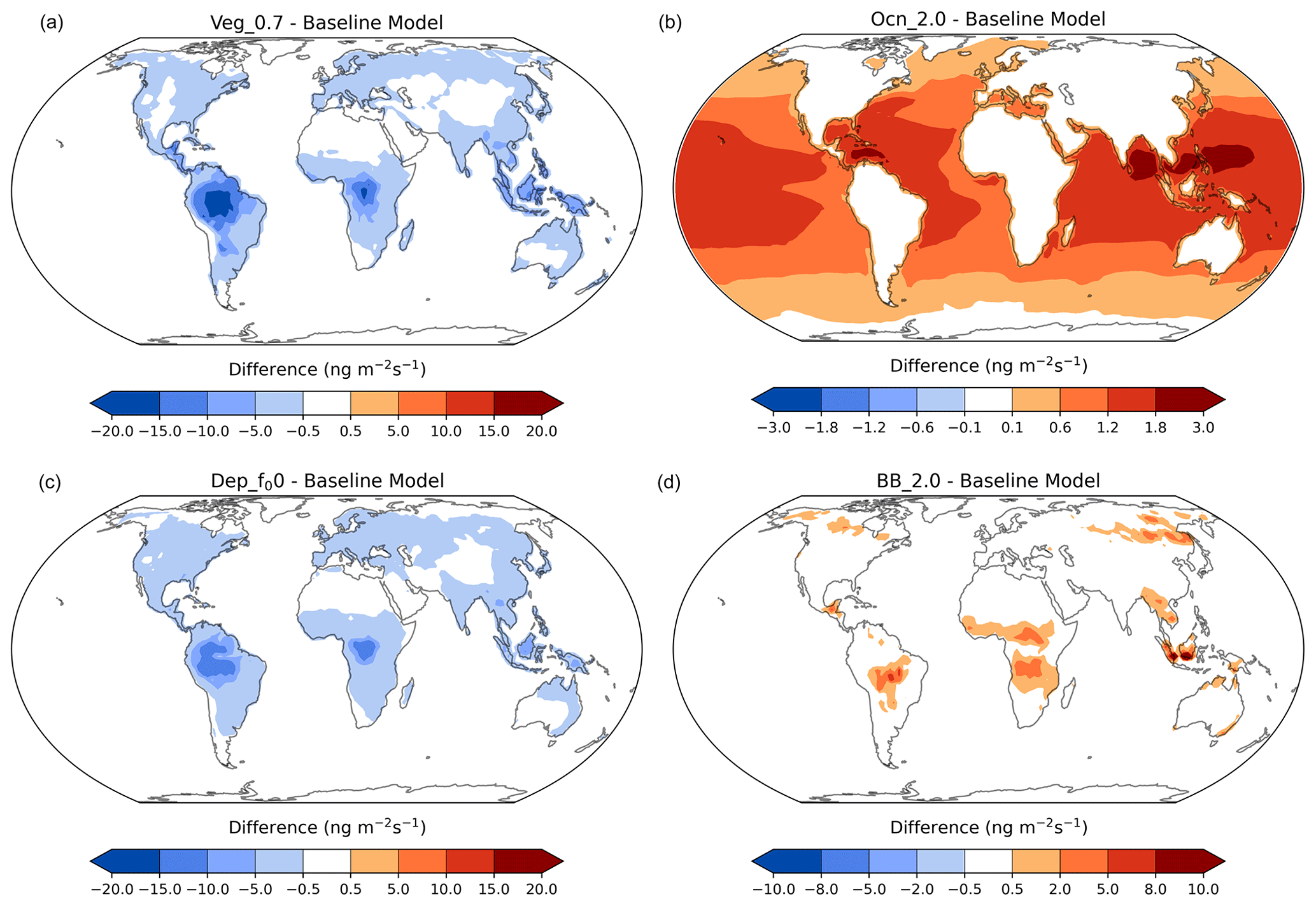
Figure 11 Acetone anomalies from the baseline simulation for the vegetation (a), ocean (b), dry-deposition (c), and biomass-burning (d) sensitivities, with red indicating an increase and blue indicating a decrease in the specific flux. Nonlinear color bars are used to better differentiate the details in the map.

Another broader finding from the ocean sensitivity study is that doubling the oceanic acetone concentration impacted oceanic emissions of acetone more than the oceanic uptake of acetone (Fig. S13). Specifically, in this sensitivity study, the emissions doubled, while the uptake increased by only 40 %. This difference may be attributed to the fact that a higher ocean concentration will generally cause less resistance in the emission direction but more resistance in the uptake direction. The differences in oceanic acetone emissions and uptakes in this sensitivity study also resulted in increased chemical destruction and an overall higher burden of acetone in the atmosphere (Fig. S13).

In the dry-deposition sensitivity simulation, the reactivity factor, f₀, was reduced from 0.1 to 0. As a result, the amount of acetone removed by deposition decreased and the atmospheric acetone concentration increased. The strongest increases were found to occur in Ispra (38.4 %), Košetice (37.9 %), Paris (37.9 %), Beijing (37.3 %), Donon (36.6 %), Mainz (33.4 %), Montelibretti (30.5 %), Rosemount (28.9 %), Berkeley (28.7 %), and Waldhof (28.7 %) (Figs. S17, S18).

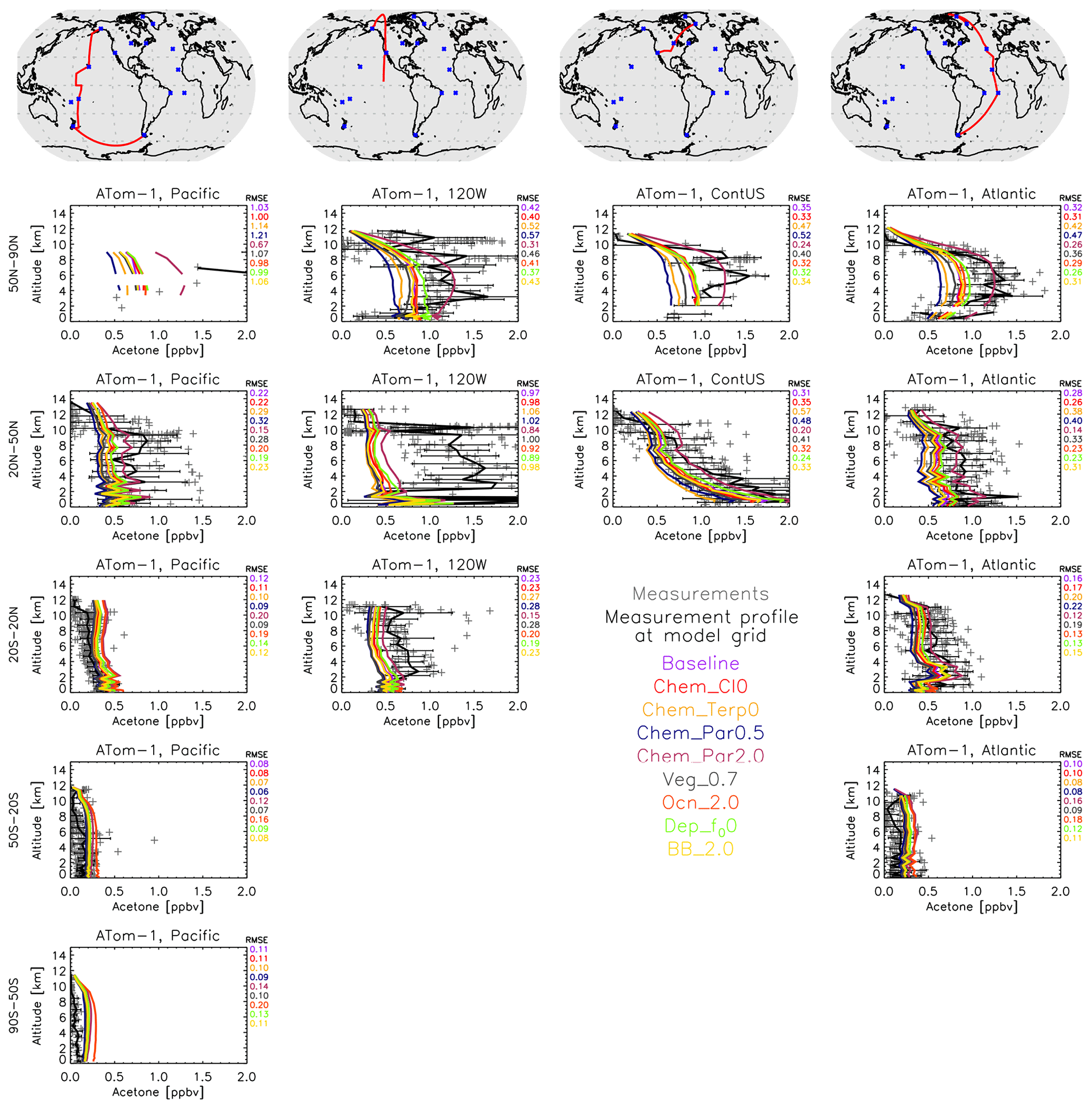
Figure 12 Similar to Fig. 8, except that a comparison between the GISS ModelE2.1 sensitivity simulations and the ATom-1 aircraft measurements (July–August 2016) is presented. Individual data points are shown with dark gray symbols, and their average values are shown in black, with error bars representing the 1-sigma range of the averages. The root mean square error (RMSE) of each simulation is noted at the top right of each panel. Note that all sensitivities are compared against the baseline simulation, not the Nudged_ATom one; however, as shown earlier, this makes very little difference in the comparison with observations (Fig. 8).

The final terrestrial flux sensitivity study, BB_2.0, doubled biomass-burning emissions. This sensitivity did not significantly change acetone mixing ratios in any of the locations studied, except for an increased summer spike (12.7 %) in Birkenes (Fig. S17). Most of the locations studied were far from biomass burning sites to begin with, however, so an analysis of this sensitivity study over biomass-burning hotspots is needed.

The acetone concentration anomalies between the terrestrial and oceanic flux sensitivity studies and the baseline simulation around the world are presented in Fig. 11. Decreasing acetone production from MEGAN vegetation by 30 % resulted in a decrease in acetone mixing ratios over the tropical and boreal forests, where this source is most prominent (Fig. 11, top left). Doubling oceanic acetone concentrations increased the production of acetone from the oceans globally. This increase was stronger in the tropics due to the higher sea surface temperatures (Fig. 11, top right). Reducing the reactivity factor for dry deposition decreased the amount of acetone removed by deposition over the continents (Fig. 11, bottom left), in particular where the acetone concentration was elevated (Fig. 3). Finally, doubling biomass-burning emissions did not change acetone mixing ratios much, other than over biomass-burning hotspots like central South America, Central Africa, Southeast Asia, and Siberia (Fig. 11, bottom right).

3.5.3 ATom comparisons

The ATom comparisons were replicated with the sensitivity simulations (Figs. 12, S19–S21). Doubling the paraffin yield of acetone seemed to have the most noticeable impacts on the vertical profiles. As seen during ATom-1 (July–August 2016), doubling the paraffin yield decreases the root mean square error (RMSE) against measurements in the Northern Hemisphere polar atmosphere and brings the model into closer agreement with observations, but it decreases the agreement throughout the remote Pacific Ocean, which implies different chemical formation pathways over the more polluted Northern Hemisphere on the Atlantic Ocean side compared to the Pacific Ocean side. Nearly the exact opposite is calculated in the case of halving the paraffin yield of acetone, which adds confidence to the chemical pathway explanation (Fig. 12). The doubling of the oceanic acetone concentration leads to a small improvement (decrease) in the RMSE over the tropical and north Atlantic Ocean during ATom-1 and an even smaller decrease over the Northern Hemisphere Pacific Ocean, but it leads to an increase over the tropical and south Pacific Ocean, showing the potential role of different oceanic concentrations of acetone across the globe (Fig. 12). It needs to be noted, though, that the model performs fairly well in those regions already, so the small improvements mentioned above do not greatly affect the regional acetone concentrations, which is also expected due to the rather weak acetone source from the ocean.

The simulations of boreal winter (January–February 2017) score the best against ATom-2 (Fig. S19). Acetone concentrations are the lowest during that period in both hemispheres. This is a direct result of the very low biomass-burning emissions, which represent one of the main acetone sources worldwide. In the region north of 50° N, the increases in both the paraffin source and the oceanic source of acetone degrade the simulations, and the same applies for the observations at around 102° W longitude, especially at mid-latitudes. The increase in the oceanic source over the Northern Hemisphere mid-latitude Pacific Ocean improves (decreases) the RMSE, but, as already mentioned, the low concentrations of acetone in that area (and in general during ATom-2) show that there is low sensitivity of the modified acetone sources to acetone profiles. While the ocean flux may be small, these ATom comparisons reveal that they especially matter in the southern latitudes. These are the same latitudes where the ocean appears to be in equilibrium (i.e., it is neither a strong source nor a strong sink) (Fig. 5).

During boreal fall (ATom-3), doubling the paraffin yield tends to cause the model to overshoot most of the observations (Fig. S20), contrary to what was calculated during boreal summer (ATom-1; Fig. 12). This is the case for most ATom-3 Atlantic Ocean flights, while an improvement is calculated when comparing with the flights near the west coast of the US or the mid-latitude Pacific Ocean. These results reveal that the model may be underestimating a paraffin source during boreal summer, which diminishes during boreal fall.

The boreal spring season (April–May 2018; ATom-4; Fig. S21) is the hardest for the model to simulate when it comes to Northern Hemisphere concentrations. All the sensitivity studies greatly underestimate observations, in particular the amount in the upper troposphere near the polar latitudes that has undergone long-range transport, but also the concentrations measured throughout the troposphere at northern mid-latitudes. The model skillfully simulates tropical and Southern Hemisphere profiles, while it cannot reproduce the higher concentrations at northern latitudes. An increased yield from paraffin or an increased oceanic concentration does reduce the RMSE, but it still falls short in capturing the magnitude, or the shape, of the profiles of the spring hemisphere. We cannot infer from our model simulations whether this is a missing source or an overestimated sink, but the latter appears to be more plausible, given the large underestimation of all modeled profiles at northern mid-latitudes. In the Southern Hemisphere, the increase in oceanic acetone clearly degrades model skill, as was frequently the case during the other campaigns presented above.

It is worth mentioning that, in most cases, the changes in the source of acetone do not alter the shape of the vertical profile. This means that the transport or chemical sinks of acetone dictate its spatiotemporal distribution more than its sources do, while the sources affect the magnitude of that distribution, and they do so quite significantly under some of the sensitivity simulations described here.

4 Conclusions

The development of acetone's representation in NASA GISS ModelE2.1 from its previous simplistic parameterization of instantaneous isoprene to a full tracer experiencing its own transport, chemistry, emissions, and deposition marks a significant improvement in the model's chemical scheme. Calculations of the 3-dimensional distribution of acetone as a function of time and evaluations of its atmospheric burden and source and sink fluxes demonstrate the complexity of acetone's spatiotemporal distribution in the atmosphere. An analysis was conducted to assess the simulated global acetone budget in the context of past modeling studies. Further comparisons were made against field observations at a variety of spatial and temporal scales, which indicated that the model agrees well with surface field measurements and vertical profiles in the remote atmosphere. The chemical formation of acetone from precursor compounds such as paraffin was found to be an uncertain yet impactful factor. Vegetation fluxes, as calculated by MEGAN, were identified as the dominant acetone source that dictates its seasonality. Additionally, the acetone concentration in seawater was found to affect oceanic sources more than oceanic sinks.

Any feedback between acetone and the rest of the chemistry, particularly ozone, was not assessed here and should be the goal of a future study. Additionally, the current ocean–acetone interaction uses a constant concentration of acetone in the ocean. It will be helpful to test a more realistic non-uniform oceanic acetone concentration when this becomes available. Finally, other atmospheric conditions such as the surface wind speed may be considered further when modifying the ocean scheme.