Evaluation of isoprene emissions from the coupled model SURFEX–MEGANv2.1

Isoprene, a key biogenic volatile organic compound, plays a pivotal role in atmospheric chemistry. Due to its high reactivity, this compound contributes significantly to the production of tropospheric ozone in polluted areas and to the formation of secondary organic aerosols.

The assessment of biogenic emissions is of great importance for regional and global air quality evaluation. In this study, we implemented the biogenic emission model MEGANv2.1 (Model of Emissions of Gases and Aerosols from Nature, version 2.1) in the surface model SURFEXv8.1 (SURface EXternalisée in French, version 8.1). This coupling aims to improve the estimation of biogenic emissions using the detailed vegetation-type-dependent treatment included in the SURFEX vegetation ISBA (Interaction between Soil Biosphere and Atmosphere) scheme. This scheme provides vegetation-dependent parameters such as leaf area index and soil moisture to MEGAN. This approach enables a more accurate estimation of biogenic fluxes compared to the stand-alone MEGAN model, which relies on average input values for all vegetation types.

The present study focuses on the assessment of the SURFEX–MEGAN model isoprene emissions. An evaluation of the coupled SURFEX–MEGAN model results was carried out by conducting a global isoprene emission simulation in 2019 and by comparing the simulation results with other MEGAN-based isoprene inventories. The coupled model estimates a total global isoprene emission of 443 Tg in 2019. The estimated isoprene is within the range of results obtained with other MEGAN-based isoprene inventories, ranging from 311 to 637 Tg. The spatial distribution of SURFEX–MEGAN isoprene is consistent with other studies, with some differences located in low-isoprene-emission regions.

Several sensitivity tests were conducted to quantify the impact of different model inputs and configurations on isoprene emissions. Using different meteorological forcings resulted in a ±5 % change in isoprene emissions using MERRA (Modern-Era Retrospective analysis for Research and Applications) and IFS (Integrated Forecasting System) compared with ERA5. The impact of using different emission factor data was also investigated. The use of PFT (plant functional type) spatial coverage and PFT-dependent emission potential data resulted in a 12 % reduction compared to using the isoprene emission potential gridded map. A significant reduction of around 38 % in global isoprene emissions was observed in the third sensitivity analysis, which applied a parameterization of soil moisture deficit, particularly in certain regions of Australia, Africa, and South America.

The significance of coupling the SURFEX and MEGAN models lies particularly in the ability of the coupled model to be forced with meteorological data from any period. This means, for instance, that this system can be used to predict biogenic emissions in the future. This aspect of our work is significant given the changes that biogenic organic compounds are expected to undergo as a result of changes in their climatic factors.

1 Introduction

Volatile organic compounds (VOCs) are a class of carbon-based chemicals known for their ability to evaporate easily at room temperature (Carroll and Kirschman, 2022). VOCs can be produced by human activities, with the primary anthropogenic sources being vehicle emissions, industrial processes, building materials, solvents, personal care products, the petroleum industry, and vehicular transport (Hester and Harrison, 1995; McDonald et al., 2018; Rajabi et al., 2020). VOCs are considered one of the most important precursors in the formation of tropospheric ozone and secondary organic aerosols (Atkinson and Arey, 2003). These chemicals play a crucial role in ground-level photochemical ozone formation by controlling oxidant production rates in areas with sufficient NO_x (nitrogen oxide) concentrations (Hester and Harrison, 1995). On a global scale, VOCs are mainly emitted from natural sources: soils, oceans, and vegetation. The VOC flux from terrestrial vegetation accounts for 90 % of the total emissions (Guenther et al., 1995). Quantitatively, the most important biogenic volatile organic compound (BVOC) is isoprene (C₅H₈). According to MEGANv2.1 (Model of Emissions of Gases and Aerosols from Nature, version 2.1) (Guenther et al., 2012), isoprene accounts for about half of all the biogenic species emitted. Isoprene is also known for its high reactivity, as it contributes considerably to the formation of ground-level ozone (Chameides et al., 1988). Monoterpenes and sesquiterpenes are also considered to be important BVOCs due to their substantial impact on the generation of atmospheric organic aerosols on a global scale (Griffin et al., 1999; Ervens et al., 2011; Shrivastava et al., 2017). The formation of ozone and atmospheric aerosols has effects that reach beyond air quality and human health concerns: they also exert a substantial influence on the current and future state of our climate (Unger, 2014a; Unger, 2014b). Consequently, achieving a precise estimation of BVOCs is of utmost importance. This precision is also crucial for making accurate forecasts of air pollutants using chemical transport models on both regional and global scales. Such precise predictions are fundamental not only for assessing air quality but also for quantifying the exact radiative forcing effects arising from ozone and aerosols under both present and future climate conditions. In this context, biogenic emissions are expected to change in the future as a response to the changing patterns of temperature, solar radiation, and land cover and use, as well as the increasing frequency and intensity of drought events. This creates a need for BVOC modelling tools that can be applied to study the present and future climate and air quality modelling assessments.

The terrestrial BVOC model used in the present study is MEGANv2.1, which is one of the most widely used models within the biogenic emission and atmospheric chemistry community for estimating the flux of biogenic organic compounds. It can be used in an offline mode but has also been coupled with other models. Several studies have been conducted implementing the MEGAN model within various canopy environment models or chemical transport models; each model has a different version and/or implementation of the MEGAN algorithms and different weather and land cover driving variables. As a result, the estimated emissions can differ considerably (the annual global isoprene emission varies between 311 and 637 Tg) (Messina et al., 2016; Henrot et al., 2017; Bauwens et al., 2018; Zhang et al., 2021).

Our scientific aim was to derive a method for estimating BVOC emissions that would be capable of considering both atmosphere and land surface processes as well as land–atmosphere interactions that impact vegetation. Therefore, our objective was to develop a modelling system for BVOCs based on MEGANv2.1 that would be flexible enough to use a variety of meteorological forcing datasets, e.g. present-day reanalyses and output from climate models for future scenarios. Furthermore, this modelling system would have to be capable of simulating impacts on vegetation arising from atmosphere–land interactions. In this study, we therefore chose to implement MEGANv2.1 within the SURFEXv8.1 (SURface EXternalisée) model, which is a land surface modelling platform developed by Météo-France in cooperation with the scientific community. While MEGANv2.1 has been coupled with SURFEX in previous work, this was done in the framework of the mesoscale atmospheric model MESO-NH (Lac et al., 2018) that includes online-coupled chemistry. We were motivated to develop this coupling further for the following reasons. First, SURFEX can be used in offline mode (i.e. using an external meteorological forcing file). Second, SURFEX includes a detailed canopy environment model called “ISBA” (Interaction between Soil Biosphere and Atmosphere) (Le Moigne, 2018). This scheme provides precise vegetation-type-dependent parameters such as soil moisture, leaf area index (LAI), vegetation fraction, and temperature. Additionally, this scheme can simulate LAI, which varies in parallel with numerous environmental and meteorological variables. Based on this dynamic LAI, the coupled model can estimate biogenic emissions interactively with leaf biomass. The latter includes alterations in the density and distribution of vegetation, thereby exerting a direct influence on the release of biogenic compounds. The impact of vegetation on climate can also be investigated through the Earth system model CNRM-ESM2-1 (Séférian et al., 2019), which includes the SURFEX land model. This effect originates from the BVOC-induced impact on aerosols and other greenhouse gas concentrations (e.g. ozone, methane), which can alter the Earth’s radiative balance (Unger, 2014a; Unger, 2014b; Sporre et al., 2019).

The SURFEX and MEGAN2.1 models are presented in Sect. 2 along with a description of the models' offline coupling. Section 3 is dedicated to the evaluation of the coupled-model isoprene emissions in comparison with other isoprene inventories. The evaluation of the sensitivity test results conducted on MEGAN's driving variables is discussed in Sect. 4.

2 Model description

2.1 SURFEX model

SURFEX (SURface EXternalisée in French) (Le Moigne, 2018) is a surface modelling platform developed by Météo-France in cooperation with the scientific community. SURFEX simulates the interaction between the surface and the atmosphere by simulating the flux exchange between the soil and the upper atmospheric layer (e.g. latent heat flux, sensible heat flux, CO₂ flux, chemical species, and aerosols). The most recent version of SURFEX (SURFEXv9.0) was released in January 2023; however, in this work, we used SURFEXv8.1, which is widely used at present (Schoetter et al., 2020; Zsebeházi and Szépszó, 2020; Schoetter et al., 2017).

SURFEX can be run in an offline mode or coupled with an atmospheric model, e.g. the global numerical weather prediction model ARPEGE (Déqué et al., 1994). Used in an online mode, SURFEX extracts the necessary meteorological data from the global weather prediction model. In offline mode, a forcing file should be prescribed as input to the model. The forcing file should contain spatio-temporal gridded maps of atmospheric variables (air temperature, specific humidity, wind components, pressure, rain rate, and CO₂) and radiative variables (solar radiation and infrared radiation). During a model time step, each surface grid box receives the forcing variables listed above; in return, SURFEX computes averaged fluxes for momentum, sensible and latent heat, chemical species, and dust fluxes, etc., and then returns these quantities to the atmosphere by adding radiative terms such as surface temperature, direct and diffuse surface albedo, and surface emissivity (Le Moigne, 2018).

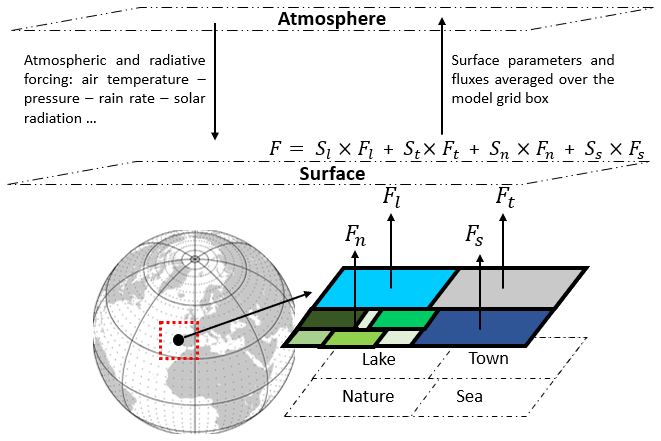
Figure 1 Grid cell representation in SURFEX and description of flux exchanges between the surface and atmospheric layer above.

As shown in Fig. 1, each grid box in SURFEX is represented by four adjacent tiles: nature, town, sea or ocean, and lakes. The final fluxes are the average of the fluxes calculated over nature, town, sea/ocean, and lake weighted by their respective fraction (S_l, S_t, S_n, S_s). SURFEX contains four principal surface schemes: ISBA for the nature tile (Calvet et al., 1998), TEB for town (Masson, 2000), FLAKE (Mironov et al., 2010) for lakes, and SEA for sea and oceans. SURFEX can also simulate aerosol chemistry and surface processes and can be used for assimilation of surface variables (Le Moigne, 2018).

To define the surface coverage, SURFEX uses ECOCLIMAP-II, which is a 1 km global database of land cover made by CNRM (Centre National des Recherches Météorlogiques, in French) (Faroux et al., 2013). It describes the types of surfaces covering the whole earth.

ECOCLIMAP-II provides the fraction data for the 19 patches (nature tile). In addition, it provides land surface parameters relative to each patch, i.e. each vegetation type has a defined soil depth, height of trees, LAI available at 10 d time steps, and vegetation fraction. LAI is represented by a 5-year averaged LAI climatology over the period 2002–2006. In ISBA, the calculation of surface parameters is based on an aggregation process at patch level (i.e. from the 19 land cover types down to the selected number of patches) for each point of the grid according to the horizontal resolution (Le Moigne, 2018).

2.2 MEGANv2.1 model

The MEGAN model is a global emission platform designed to estimate the net emission of gases and aerosols from terrestrial ecosystems into the atmosphere. It is an updated version of MEGANv2.0, developed by Guenther et al. (2006) to estimate isoprene flux, and MEGAN2.02, which was described for monoterpene and sesquiterpene emissions by Sakulyanontvittaya et al. (2008).

MEGANv2.1 (the model's routines and input data can be found at https://bai.ess.uci.edu/megan/data-and-code/megan21, last access: 8 September 2023) includes algorithms that take into account the main known processes controlling biogenic emissions; it makes it possible to estimate the flux of 19 compound classes, which are decomposed into 147 individual species such as isoprene, monoterpenes, sesquiterpenes, carbon monoxide, alkanes, alkenes, aldehydes, acids, ketones, and other oxygenated VOCs (Guenther et al., 2012). These species can then be lumped into the appropriate categories for the chemical scheme for use in chemical transport models. The stand-alone version of MEGANv2.1 requires as input weather data (temperature, precipitation, solar radiation, wind, and photosynthetic photon flux), atmospheric chemical composition data (CO₂ concentration), land cover data (plant functional type distribution and LAI data), and emission factor data.

The estimation of biogenic fluxes in MEGANv2.1 is based on a simple equation (Eq. 1) to calculate the net primary emission flux from terrestrial landscapes (F_i) into the above-canopy atmosphere ($\mathrm{\mu }{\mathrm{m}}^{-\mathrm{2}}{\mathrm{s}}^{-\mathrm{1}}$). This equation comprises two significant components: firstly, the emission factor, which represents the emission potential of a specific compound associated with a particular vegetation type, and secondly, the emission activity factor, which reflects how this emission potential responds to variations in environmental conditions and meteorological conditions.

$$\begin{array}{}\text{(1)}& F_i={\mathit{\gamma }}_i\times \sum _{j=\mathrm{1}}^n({\mathit{\epsilon }}_{ij}\times {\mathit{\chi }}_j),\end{array}$$

where γ_i is the dimensionless activity factor of a compound i (this factor is equal to 1 in standard conditions described below), ε_ij is the emission potential (also known as “emission factor”) of a compound i and vegetation type j at standard conditions, and χ_j is the fractional grid box areal coverage.

2.2.1 Vegetation and emission factor

A grid cell in MEGANv2.1 is represented by different types of vegetation also called “plant functional types” (PFTs). A distribution of 16 PFTs is used to represent the vegetation cover, consistent with the vegetation categories used in the Community Land Model version 4 (CLM4) (Gent et al., 2011), which is a model used to simulate the interactions between the surface and the atmosphere.

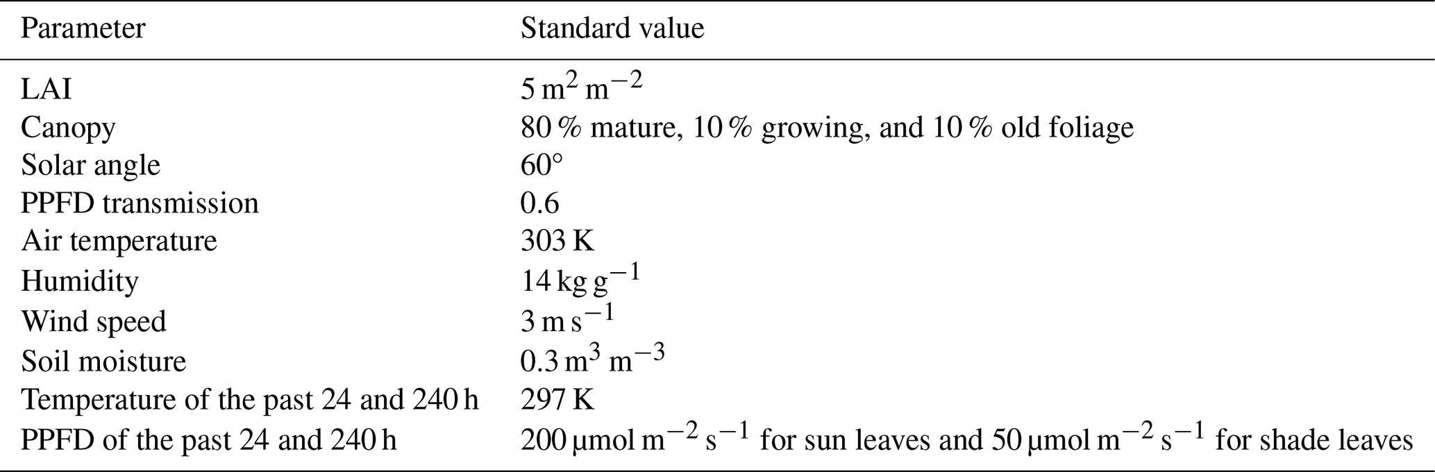
The emission factor represents the potential of a vegetation type to emit a specific chemical species under standard conditions. The list of standard conditions used in MEGANv2.1 is shown in Table 1. These conditions are relative to vegetation (e.g. LAI, growing and mature foliage fractions), meteorology (e.g. solar angle, Photosynthetic Photon Flux Density (PPFD) transmission, temperature, humidity, wind speed), soil (e.g. soil moisture) and canopy (e.g. the past 24 and 240 h temperature and PPFD for sun and shade leaves).

The estimation of BVOCs in MEGANv2.1 can be made by using a global gridded high-resolution emission potential map prescribed as input to the model (this map is provided with the MEGAN code for 10 predominant biogenic species) or by using PFT spatial coverage and PFT-dependent emission potential data.

Table 1 List of standard conditions used in MEGANv2.1 (Guenther et al., 2006).

2.2.2 Emission activity factor

The emission activity factor represents the response of the vegetation to a change in environmental and meteorological conditions. The activity factor γ_i of a compound class i is calculated in the MEGANv2.1 Fortran code as the multiplication of factors accounting for emission response to light γ_P,i, temperature γ_T,i, leaf age γ_A,i, soil moisture γ_SM,i, LAI, and CO₂ inhibition ${\mathit{\gamma }}_{{\mathrm{CO}}_{\mathrm{2}},i}$ as follows:

$$\begin{array}{}\text{(2)}& {\mathit{\gamma }}_i=C_{\mathrm{CE}}\times \mathrm{LAI}\times {\mathit{\gamma }}_{P,i}\times {\mathit{\gamma }}_{\mathrm{T},i}\times {\mathit{\gamma }}_{\mathrm{A},i}\times {\mathit{\gamma }}_{\mathrm{SM},i}\times {\mathit{\gamma }}_{{\mathrm{CO}}_{\mathrm{2}},i}.\end{array}$$

The canopy environment coefficient C_CE is used to normalize the activity factor at the standard conditions listed above and is dependent on the canopy environment model being used. In MEGANv2.1 code, the equation used to calculate γ_i is

$$\begin{array}{}\text{(3)}& \begin{array}{rl}{\mathit{\gamma }}_i& ={\mathit{\gamma }}_{\mathrm{A},i}\times {\mathit{\gamma }}_{\mathrm{SM},i}\times {\mathit{\gamma }}_{{\mathrm{CO}}_{\mathrm{2}}}\\ & \times \left(\right(\mathrm{1}-\mathrm{LDF})\times {\mathit{\gamma }}_{\mathrm{TLI},i}\times {\mathit{\gamma }}_{\mathrm{LAI},i}+\mathrm{LDF}\times {\mathit{\gamma }}_{\mathrm{TLD},i}),\end{array}\end{array}$$

where γ_TLI,i is the sum of the temperature light-independent activity factor at five canopy levels and γ_TLD,i is the sum of the product of the light activity factor and the temperature light-dependent activity factor at five canopy levels. In fact, in MEGANv2.1 the emission of each compound class includes a light-dependent fraction (LDF) and a light-independent fraction (LIF = 1 − LDF) that is not influenced by light. Each compound has a specific LDF (for isoprene: LDF = 1). Light-dependent emissions are calculated following the isoprene response to temperature described by Guenther et al. (2006), and light-independent emissions follow the monoterpene exponential temperature response described by Guenther et al. (1993). The calculation of light-dependent and light-independent factors is based on a detailed canopy environment model that estimates light (PPFD), temperature (T), and the fraction of sun and shade leaves at five canopy levels. The calculation of γ_TLI,i and γ_TLD,i is presented in Eqs. (4), (5), (6), and (7), where ${\mathit{\gamma }}_{\mathrm{TLI}}^j$ and ${\mathit{\gamma }}_{\mathrm{TLD}}^j$ are calculated as the sum of the temperature light-independent factor and the light-dependent factor respectively weighted by the fraction of sun leaves $f_{\mathrm{sun}}^j$ and the fraction of shade leaves ($\mathrm{1}-f_{\mathrm{sun}}^j$) in each canopy level.

$$\begin{array}{}\text{(4)}& {\displaystyle }{\mathit{\gamma }}_{\mathrm{TLI}}=\sum _{j=\mathrm{1}}^{\mathrm{5}}{\mathit{\gamma }}_{\mathrm{TLI}}^j\text{(5)}& {\displaystyle }{\mathit{\gamma }}_{\mathrm{TLI}}^j={\mathit{\gamma }}_{\mathrm{TI},\mathrm{sun}}\times f_{\mathrm{sun}}^j+{\mathit{\gamma }}_{\mathrm{TI},\mathrm{shade}}\times (\mathrm{1}-f_{\mathrm{sun}}^j)\text{(6)}& {\displaystyle }{\mathit{\gamma }}_{\mathrm{TLD}}=C_{\mathrm{CE}}\times \mathrm{LAI}\times \sum _{j=\mathrm{1}}^{\mathrm{5}}{\mathit{\gamma }}_{\mathrm{TLD}}^j\text{(7)}& {\displaystyle }\begin{array}{rl}{\mathit{\gamma }}_{\mathrm{TLD}}^j& ={\mathit{\gamma }}_{P,\mathrm{sun}}\times {\mathit{\gamma }}_{\mathrm{TD},\mathrm{sun}}\times f_{\mathrm{sun}}^j+{\mathit{\gamma }}_{P,\mathrm{shade}}\times {\mathit{\gamma }}_{\mathrm{TD},\mathrm{shade}}\\ & \times (\mathrm{1}-f_{\mathrm{sun}}^j)\end{array}\end{array}$$

The calculation of γ_TI,sun, γ_TI,shade, $f_{\mathrm{sun}}^j$, γ_P,sun, γ_TD,sun, γ_P,shade, and γ_TD,shade is detailed in Guenther et al. (2012).

2.3 SURFEX–MEGAN coupling

The coupling of MEGAN2.1 and SURFEXv8.1 is based on a previous implementation of MEGAN in MESO-NH5.4. MESO-NH5.4 is an atmospheric non-hydrostatic research model designed for studies of physics and chemistry (Lac et al., 2018). This coupling involved merging MEGAN routines and linking the required inputs of the biogenic model with the SURFEX parameters.

The present study focuses on the online integration of MEGAN into SURFEX. The ultimate aim of this coupling is to be able to force the coupled model through various climate change scenarios in order to assess the climate change impact on the biosphere and to quantify the effect of these changes on biogenic emissions and therefore on global and local air quality. Additionally, this coupling aims to improve biogenic emission estimations by providing the MEGAN model with detailed vegetation-dependent inputs at patch level. This allows key land surface parameters used by MEGAN, i.e. leaf area index and soil moisture, to be calculated at a more precise scale. Thus, activity factors are individually calculated for each patch. This approach allows for a more accurate representation of biogenic emissions in the context of climate change and of their impact on air quality.

Table 2 Description of the mapping between CLM4 and ECOCLIMAP vegetation types. The 16 PFTs are grouped into 6 vegetation types (NT: needleleaf trees, BT: broadleaf trees, SHRB: shrubs, GRLD: grassland, CROP: crops). Five ECOCLIMAP patches are not included in this list, as they represent patch 1 = bare soil; patch 2 = rock; patch 3 = snow; patch 9 = irrigated crops; and patch 12 = peat bogs, parks, and gardens.

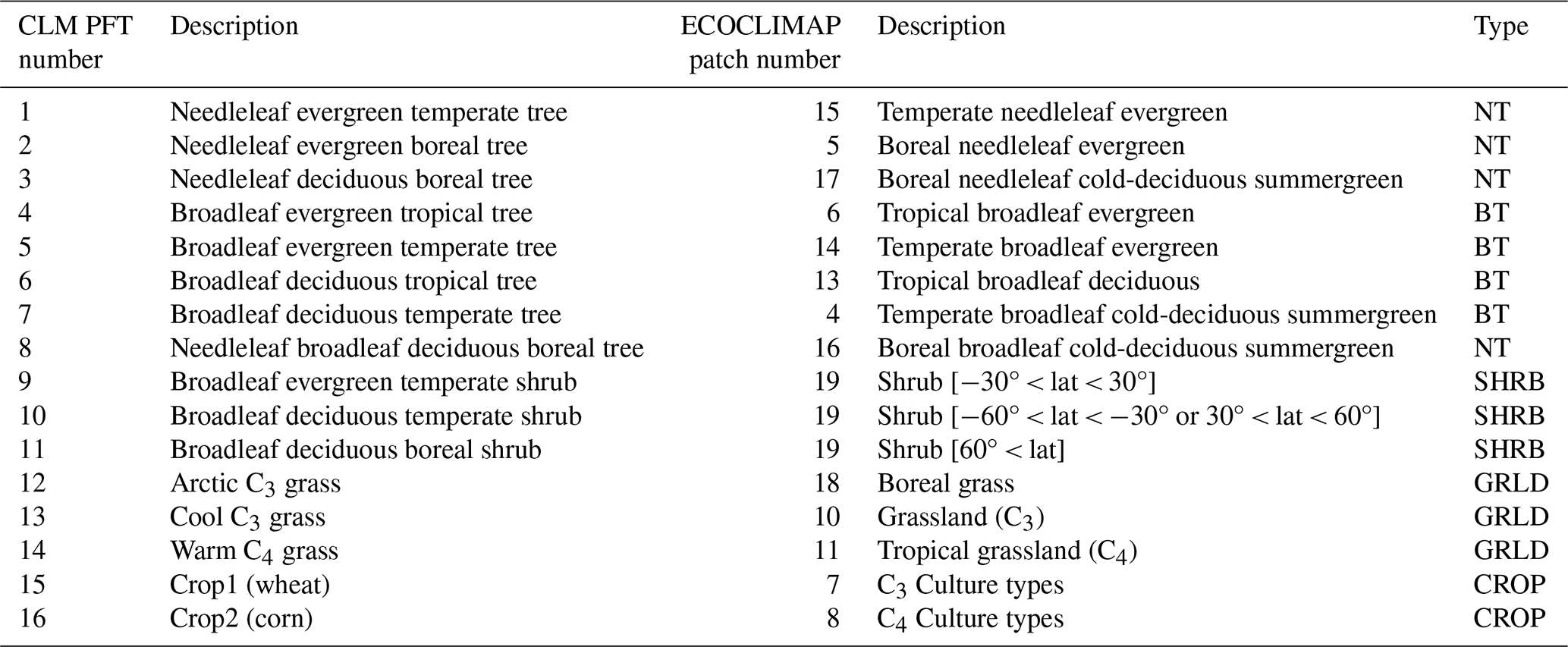
In the coupled model the estimation of biogenic fluxes of various species was carried out based on 16 vegetation types extracted from the ECOCLIMAP-II database (Faroux et al., 2013). Each vegetation type from ECOCLIMAP-II was mapped to its corresponding type defined in CLM4. Table 2 represents the mapping used in the coupled model. For most CLM4 PFTs, similar existing vegetation types are defined in ECOCLIMAP-II. However, when considering shrubs, CLM4 classifies them into three distinct categories: evergreen temperate shrub, deciduous temperate shrub, and broadleaf deciduous shrub. Conversely, ECOCLIMAP-II does not provide separate classifications for these three distinct types of shrubs. To overcome this limitation, the three plant functional types corresponding to the different types of shrubs were introduced in ECOCLIMAP-II by assigning the shrub patch to a specific geographical area based on a given latitudinal range. The evergreen temperate shrub type is specified in the coupled model as the shrub patch in tropical regions (−30° < latitude < 30°), the deciduous temperate shrub in temperate regions (−60° < latitude < −30° or 30° < latitude < 60°), and the deciduous boreal shrub in boreal regions (60° < latitude). This approach allows for a more accurate representation of shrubs in the coupled model.

Figure 2 represents a comparison between the vegetation types used in the MEGAN stand-alone version and the ones defined in ECOCLIMAP-II. For comparison, we have grouped the 16 PFTs into 6 main vegetation types: broadleaf evergreen trees, needleleaf evergreen trees, deciduous trees, shrubs, grassland, and crops. The vegetation spatial distribution and intensity are similar for most vegetation types in ECOCLIMAP-II and CLM4. For shrubs, the substantial difference in vegetation distribution is due to the vegetation height threshold used in ECOCLIMAP-II (2 m) and in CLM4 (10 m). For other vegetation types (e.g. needleleaf trees), the difference in vegetation density between ECOCLIMAP and CLM4 is expected to have a small impact on isoprene emissions, as this specific PFT represents only 1.4 % of the total annual emitted isoprene (Guenther et al., 2012). For vegetation-related input data, MEGAN can use climatological LAI from the ECOCLIMAP-II database; in this case, the LAI is defined for each vegetation type in a 10 d time step, or the dynamic LAI is estimated for each vegetation type with the vegetation scheme in SURFEX. LAI_v, defined as the LAI in a grid cell divided by the vegetation fraction, is considered equal to the current LAI, and LAI_p (previous LAI) is defined as the LAI value of 10 d in the past.

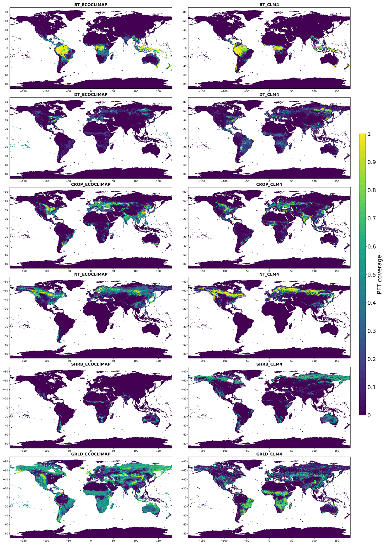
Figure 2 Spatial coverage of the six vegetation types defined in Table 2: BT (broadleaf trees), NT (needleleaf trees), DT (deciduous trees), GRLD (grassland), SHRB (shrubs), and CROP (crops) in CLM4 (right) and in ECOCLIMAP-II (left).

In the SURFEX model time step, all surface variables are interpolated and updated for each grid cell. Each tile is treated independently by using a specific scheme. For the nature tile, the surface parameters are calculated following the vegetation-type aggregation process, which merges several vegetation types into a single patch (ranging from 1 to 19).

It is important to clarify that the coupling of SURFEX and MEGAN is online, which means that MEGAN's estimation of biogenic fluxes interacts dynamically with the ISBA scheme (Interaction between Soil Biosphere and Atmosphere). ISBA is the scheme used for the nature tile to compute the exchanges of energy and water between the soil–vegetation–snow continuum and the atmosphere above.

The online implementation of MEGAN was done following the SURFEX conceptual framework, which separates the initialization phase from the temporal evolution phase. This involved setting up specific routines to initialize and interpolate MEGAN-related parameters (e.g. emission factors). The temporal estimation of biogenic emissions was carried out as an integral part of the ISBA scheme. This was achieved by integrating MEGAN routines that estimate the activity factor for each vegetation patch, using vegetation parameters estimated by ISBA, which encompass factors like soil moisture and wilting point at different layers (depending on the soil discretization method), leaf area index, photosynthetically active radiation (PAR), and surface temperature. Figure 3 shows a global representation of the online implementation of MEGAN in SURFEX.

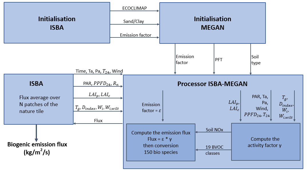
Figure 3 Schematic description of the SURFEX–MEGAN coupling. T_a is the air temperature at 2 m height, P_a is the surface pressure, T₂₄ and PPFD₂₄ are the previous day mean temperature and PPFD respectively, W_i and W_i,wilt are the soil moisture and wilting point at different soil layers respectively, T_g is the soil surface temperature, ϵ is the emission factor, γ is the activity factor, R_n is the incoming short-wave solar radiation flux, LAI_p and LAI_c are the LAI value of the previous and current day respectively, and D_index is the soil category.

3 Evaluation of SURFEX–MEGAN flux estimates

3.1 Model setup

The coupled SURFEX–MEGAN model was utilized to conduct a global simulation of isoprene emissions in 2019 using ERA5 meteorological forcing. This simulation is referred to as the “reference simulation” (abbreviated as REF).

ERA5 is a reanalysis based on the integrated forecasting system IFS (numerical weather forecasting model and data assimilation system developed jointly by ECMWF and Météo-France) (Hersbach et al., 2020). For the REF SURFEX–MEGAN simulation, the ERA5 forcing file includes hourly reanalysis meteorological fields defined on a 1°×1° spatial resolution grid (re-gridded from the native 31 km × 31 km resolution). Temperature and specific humidity were extracted at 2 m height; wind speed and wind direction were calculated based on zonal and meridian wind components at 10 m height. As there are no available inputs for surface incident diffuse short-wave radiation and CO₂ rate, these parameters were assigned values of 0 W m⁻² and 410 ppm respectively. The CO₂ concentration value corresponds to the 2019 annual mean CO₂ observed at Mauna Loa (Keeling et al., 2005).

In this study, the calculation of PPFD and temperature for sun and shade leaves at different canopy heights was made using the canopy model integrated in MEGAN; the incoming PAR (photosynthetically active radiation) at the top of the canopy was assumed to be 48 % of the incoming short-wave radiation (Jacovides et al., 2003) (Nagaraja Rao, 1984), and a conversion factor of 4.6 and 4.0 µmol photons J⁻¹ was used to convert PAR to PPFD for diffuse and direct radiation respectively (Guenther et al., 2012). Unless otherwise stated, in all coupled model simulations the estimation of isoprene flux was based on the isoprene potential map, and the effect of soil moisture deficit and CO₂ on BVOC emissions was not taken into account (the γ_SM and ${\mathit{\gamma }}_{{\mathrm{CO}}_{\mathrm{2}}}$ factors were assigned a value of 1). This choice enables a better comparison with other emission inventories. Additionally, the impact of the CO₂ inhibition factor becomes relevant only when CO₂ atmospheric concentrations exceed 400 ppmv significantly (Sindelarova et al., 2014).

For simplicity, we have used the ISBA 2-L scheme in the present study. In this scheme, the soil is represented with two layers, and the heat and moisture exchanges between the layers and the atmosphere are modelled with the force-restore method (Le Moigne, 2018); this approach is described further in Sect. 4.

3.2 Comparison of SURFEX–MEGAN isoprene emissions with other datasets

3.2.1 Isoprene inventory description

The validation of the results obtained by the coupled model was benchmarked by comparing the 2019 global and regional isoprene emission results with other isoprene inventories estimated with the MEGAN model. The data used for this comparison are presented in Table 3; additional information regarding the simulation setup used to generate the results is also provided. For inventories with unavailable 2019 isoprene emissions, the closest available year was used for comparison. It should be noted that this evaluation does not include a comparison with real-world observations, as the MEGAN model was thoroughly discussed in other papers aiming to validate the MEGAN model estimations of local isoprene flux measurements (Sindelarova et al., 2014; Situ et al., 2014; Kota et al., 2015; Seco et al., 2022).

Table 3 List of isoprene inventories used for the model validation and description of driving input data; α is the conversion factor used to approximate PAR from downward surface solar radiation = 0.45; (a) Sindelarova et al. (2022), (b) Sindelarova et al. (2014), (c) Opacka et al. (2021).

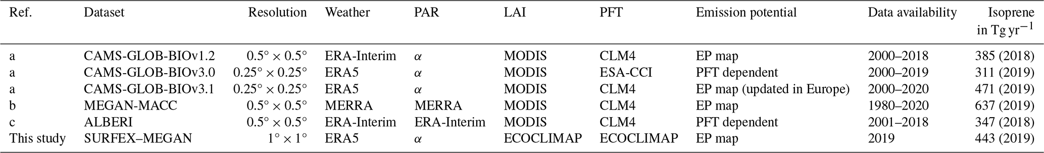
CAMS-GLOB-BIO is a high-resolution global emission inventory of the main biogenic species including isoprene, monoterpene, sesquiterpenes, methanol, acetone, and ethene (Sindelarova et al., 2022). It provides monthly average inventories and monthly average daily profiles of three different emission scenarios for the period 2000–2019. CAMS-GLOB-BIOv1.2 is a 0.5°×0.5° spatial resolution dataset obtained with ERA-Interim meteorology, the vegetation cover is based on the CLM4 16 PFTs, and the emissions are calculated based on the emission potential map provided with the MEGANv2.1 code. CAMS-GLOB-BIOv3.0 and CAMS-GLOB-BIOv3.1 have a higher spatial resolution of 0.25°×0.25° and are based on the ERA5 meteorology. The aim of the 3.0 scenario is to capture the impact of the land cover annual evolution on biogenic emissions by using the land cover data provided by the Climate Change Initiative of the European Space Agency (ESA-CCI). The 3.1 scenario uses the CLM4 vegetation cover and emission potential map for isoprene and the main monoterpenes. The EP (emission potential) map was updated over Europe using high-resolution land cover maps and detailed information of tree species composition and emission factors from the EMEP MSC-W model system.

MEGAN-MACC is a biogenic emission inventory developed under the Monitoring Atmospheric Composition and Climate project (MACC) (Sindelarova et al., 2014). It includes monthly mean emissions of 22 biogenic species (isoprene, monoterpenes, sesquiterpenes, methanol, and other oxygenated VOCs and carbon monoxide) estimated by the MEGANv2.1 model on a global 0.5°×0.5° grid for the period 1980–2020 using meteorological fields of Modern-Era Retrospective Analysis for Research and Applications (MERRA).

The ALBERI dataset is a bottom–up inventory of isoprene emissions developed in the framework of the ALBERI project funded by the Belgian Science Policy Office (Opacka et al., 2021). Isoprene emissions are estimated by the MEGANv2.1 model coupled with the canopy environment model MOHYCAN (Model for Hydrocarbon emissions by the CANopy) (Wallens, 2004) (Bauwens et al., 2018). The model was driven by the ERA-Interim meteorological fields, and vegetation description was provided from satellite-based Land Use and Land Cover (LULC) datasets at annual time steps. The LULC datasets are based on the MODIS PFT dataset and are adjusted to match the tree cover distribution from the Global Forest Watch (GFW) database (Hansen et al., 2013).

3.2.2 Spatio-temporal distribution analysis

The global annual isoprene emission estimated with SURFEX–MEGAN simulation is 443 Tg. The isoprene estimates of the coupled model fall within the range of previous reported values calculated with MEGANv2.1, varying between 311 and 637 Tg. The discrepancies between isoprene totals obtained by different studies are due to many factors, including model assumptions and input data (e.g. meteorology, LAI, vegetation distribution). In fact, according to Messina et al. (2016), isoprene emissions are highly dependent on LAI, as they linearly increase up to LAI = 2 m² m⁻² and then gradually decrease to become almost constant above 5 m² m⁻². As shown by Sindelarova et al. (2014), the use of different LAI inputs (MERRA reanalysis data instead of MODIS LAI data) can lead to a 4 % increase in annual isoprene emissions. The use of different data of photosynthetically active radiation (PAR) can also significantly impact the calculated isoprene emissions. Sindelarova et al. (2014) found that using PAR derived from the MERRA incoming short-wave radiation, instead of PAR provided by the MERRA land model, led to a 17.5 % increase in total isoprene emissions. Later in this section, we examine other individual factors responsible for the total isoprene discrepancies and the differences in spatio-temporal distribution between isoprene estimates from SURFEX–MEGAN and other isoprene inventories.

Figure 4 displays the annual mean isoprene flux of the six inventories. As shown in Fig. 4, the spatial distribution of isoprene shows similar general spatial patterns for the different datasets, with important isoprene emissions located in South America (the Amazon rainforest) and Africa (the Congo rainforest); however, some differences can be discerned in Australia as well as in the maximum isoprene emission estimated by each inventory. These discrepancies can be attributed to the emission potential data used in each simulation and the PFT cover present in the area, as the spatial distribution of isoprene can be highly impacted by both the model assumptions regarding emission capacity and the spatial distribution of the vegetation types considered.

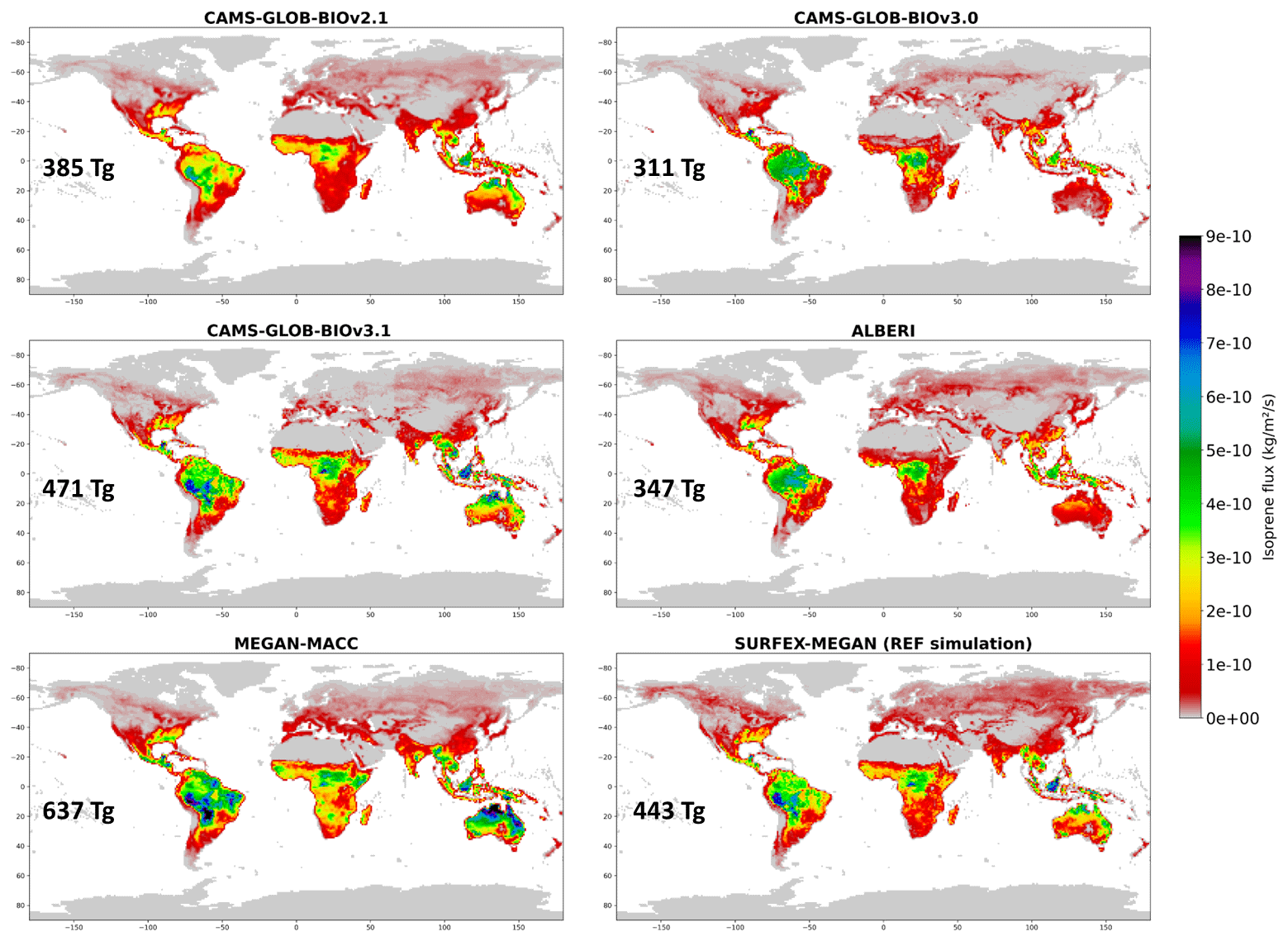
Figure 4 Spatial distribution of annual mean isoprene flux (kg m⁻² s⁻¹) of CAMS-GLOB-BIOv1.2, CAMS-GLOB-BIOv3.0, CAMS-GLOB-BIOv3.1, MEGAN-MACC, ALBERI, and SURFEX–MEGAN in 2019 (2018 for CAMS-GLOB-BIOv1.2 and ALBERI).

The isoprene flux in the SURFEX–MEGAN simulation shows a comparable spatial pattern to CAMS-GLOB-BIOv3.1. This similarity can be attributed to the fact that both simulations use ERA5 meteorological forcing, the same isoprene emission potential gridded map, and similar vegetation distributions (cf. Sect. 2.3). The isoprene emissions in MEGAN-MACC also show similar spatial patterns, with more significant emissions located in Australia and South America. By contrast, the spatial distribution of isoprene in CAMS-GLOB-BIOv3.0 and ALBERI differs significantly from that of the SURFEX–MEGAN simulation, as these two simulations were produced using the PFT-dependent emission potential table from MEGAN.

In other regions of the globe, such as North America, Europe, and North Asia, isoprene emissions from SURFEX–MEGAN are particularly higher when compared with other isoprene inventories. This discrepancy can be attributed to variations in vegetation types and their intensity between CLM4 and ECOCLIMAP in these specific areas. As shown in Fig. 2, needleleaf trees and grassland density in Asia and North America are notably greater in ECOCLIMAP, making the emissions in these regions substantially higher in SURFEX–MEGAN compared with other CLM4 PFT-based isoprene inventories.

Figure 5 represents the time series of global monthly isoprene in 2019 of SURFEX–MEGAN compared to the five other inventories. The monthly variation in isoprene emissions in the SURFEX–MEGAN simulation is marked by small monthly fluctuations. The maximum isoprene emission occurs in boreal summer (July/August) with a total isoprene of 40 Tg and the minimum in boreal winter (February) with a total isoprene of 33 Tg. The annual cycle of SURFEX–MEGAN isoprene is in agreement with the ALBERI and CAMS-GLOB-BIOv1.2 datasets. A visible shift is noticed for MEGAN-MACC and CAMS-GLOB-BIOv(3.0–3.1) isoprene annual cycles, with peak concentrations occurring in December/January and minimum concentrations in May/June.

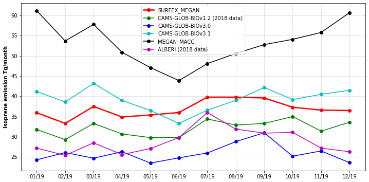
Figure 5 Global monthly isoprene (Tg month⁻¹) from the six different datasets in 2019. The 2018 data were used for CAMS-GLOB-BIOv1.2 and ALBERI.

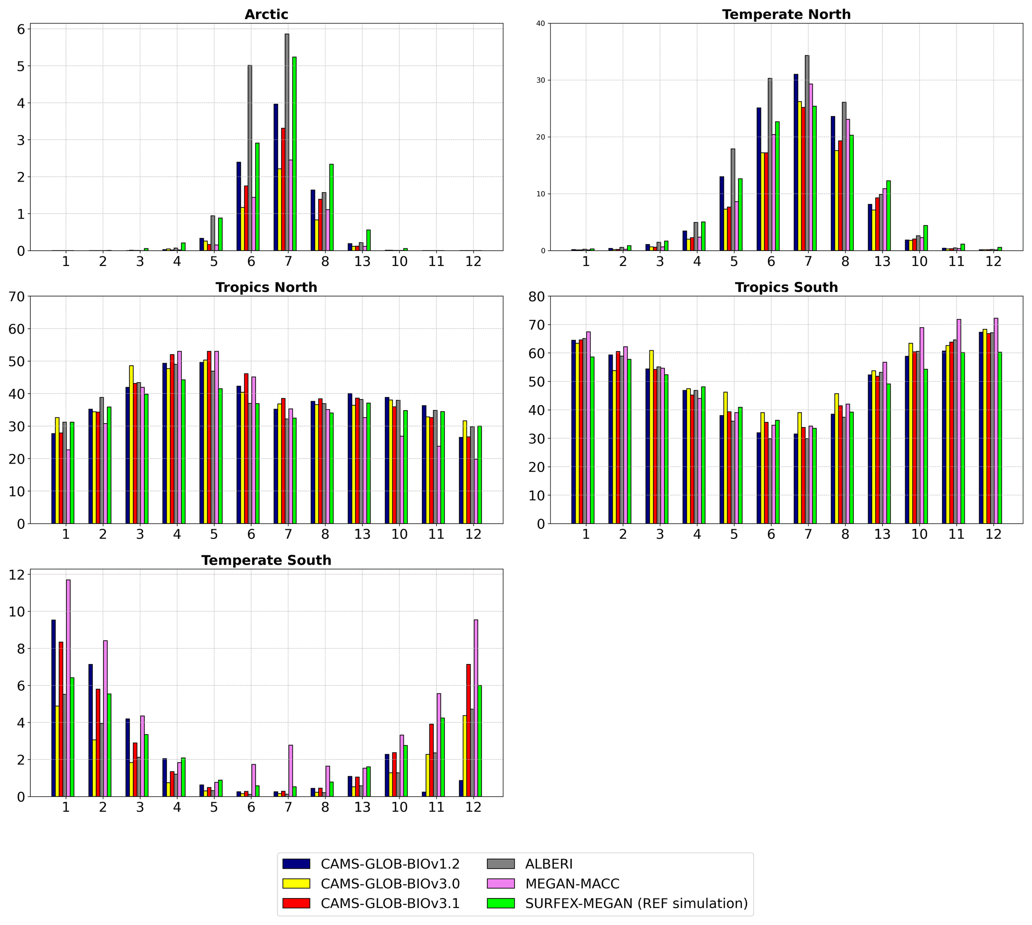
Figure 6 Contribution of zonal regions to monthly isoprene in CAMS-GLOB-BIOv1.2, CAMS-GLOB-BIOv3.0, CAMS-GLOB-BIOv3.1, MEGAN-MACC, ALBERI, and SURFEX–MEGAN simulations in 2019 (2018 for CAMS-GLOB-BIOv1.2 and ALBERI). The zonal bands are defined as Arctic (90 and 60°), temperate north (60 and 30°), tropics north (30 and 0°), tropics south (0°, −30°), temperate south (−30 and −60°).

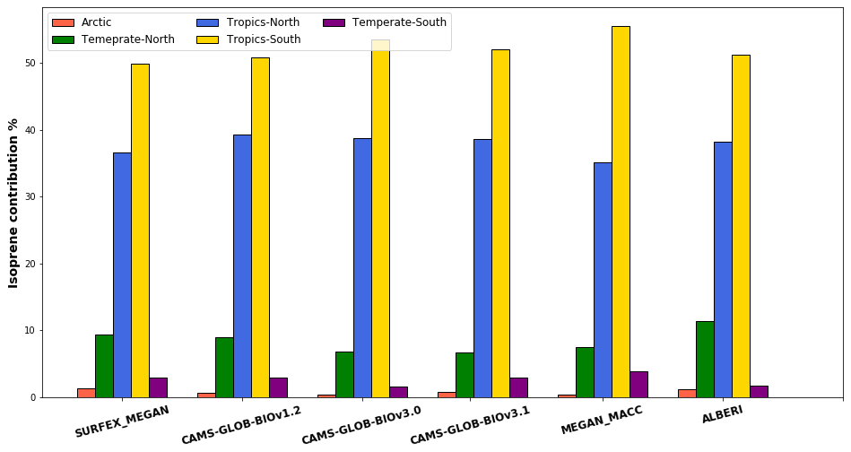
Figure 7 Contribution of zonal regions to annual isoprene for different emission datasets in 2019 (2018 for CAMS-GLOB-BIOv1.2 and ALBERI).

Figures 6 and 7 represent respectively the monthly and yearly relative contribution of different zonal regions to isoprene emissions for the different datasets. In the SURFEX–MEGAN simulation, the annual cycle of isoprene follows the seasonal cycle: in boreal summer (May–June–July–August), isoprene emissions are preponderant in the Northern Hemisphere (60 % of total emissions in this period) and in austral summer (October–November–December–January–February), isoprene emissions are preponderant in the Southern Hemisphere (64 % of total emissions in this period). As shown in Fig. 6, the southern and northern tropical regions predominate throughout the year. Their contribution to the total emissions in the SURFEX–MEGAN simulation varies between 33 %–60 % and 30 %–44 % respectively; this is due to the meteorological conditions that are favourable throughout the year (both in terms of temperature and solar radiation) and due to the high concentration of vegetation in these areas. Northern temperate regions are only active during boreal summer, with a maximum contribution of 24 % in July. The contribution of southern temperate regions follows a cyclical pattern, with a maximum in austral summer (6 % in the reference simulation). Finally, the Arctic is characterized by a very low flux, which is due to the unfavourable weather conditions and relatively low vegetation cover.

The monthly variation in isoprene emissions is strongly influenced by the contribution of the emitting regions throughout the year. As already mentioned, southern tropical regions are active throughout the year for all isoprene datasets, with particularly high contributions during November/December and lower contributions during June/July. As shown in Fig. 7, southern tropical regions account for approximately 49 % of annual isoprene emissions in SURFEX–MEGAN and CAMS-GLOB-BIOv1.2. However, their contribution to the annual isoprene flux is significantly higher in MEGAN-MACC (56 %) and CAMS-GLOB-BIOv(3.0–3.1) (54 %–52 %), which can explain the peak in isoprene emissions observed during November/December. Conversely, isoprene emissions from northern temperate regions are relatively higher in SURFEX–MEGAN (10 %), CAMS1.2 (9 %), and ALBERI (11 %) when compared with MEGAN-MACC (7 %) and CAMS3.0/3.1 (6 %). These regions are emitting mainly during boreal summer, which can explain the isoprene peak observed during July for SURFEX–MEGAN/CAMS1.2/ALBERI.

The isoprene spatial and temporal distributions of the SURFEX–MEGAN coupled model are in agreement with other MEGAN-driven isoprene inventories. The evaluation of the total annual isoprene is, however, difficult to assess, as the emissions are highly affected by both model input data and model assumptions.

4 SURFEX–MEGAN isoprene sensitivity tests

In order to analyse isoprene emission variations linked to the driving parameters of MEGAN, three sensitivity tests were conducted. As reported in (Guenther et al., 2012), isoprene emissions depend on various meteorological and environmental parameters as well as on the model assumptions. In this study, we investigated isoprene emission sensitivity to meteorology using two different additional meteorological datasets (both IFS and MERRA) (S1), analysed isoprene emissions with a different set of emission potentials (S2), and studied the impact of soil moisture on isoprene emissions (S3). Table 4 summarizes the list of sensitivity tests performed in this study, along with a description of each test setup. The impact of each sensitivity test was examined on the global and regional scales by analysing the annual isoprene emission contribution from nine geographical regions defined in the GlobEmission project (https://www.globemission.eu/, last access: 15 January 2024). The spatial extent of the regions is given in Fig. 8.

Table 4 List of sensitivity runs performed.

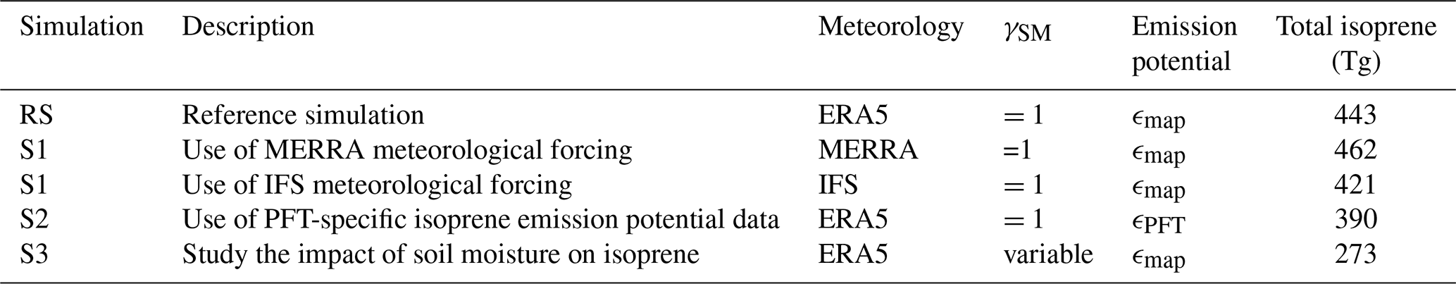
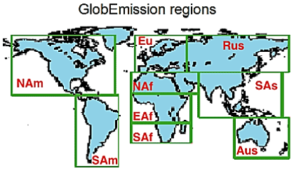
Figure 8 Geographical extent of the GlobEmission regions (NAm: North America, SAm: South America, Eu: Europe, NAf: Northern Africa and Middle East, EAf: East Africa, SAf: Southern Africa, Rus: Russia, SAs: South East Asia, Aus: Australia); from Sindelarova et al. (2014).

4.1 Meteorology

The emission rate of isoprene can be influenced by a variety of meteorological factors, including temperature, solar radiation, and atmospheric humidity. To illustrate the impact of these factors on isoprene emission estimated by SURFEX–MEGAN, two simulations were conducted using two meteorological datasets: IFS forecast dataset (operational real-time weather forecast, forecast grid data) and MERRA. MERRA was undertaken by NASA’s Global Modelling and Assimilation Office. The data were generated with version 5.2.0 of the Goddard Earth Observing System (GEOS) atmospheric model and data assimilation system (DAS) and cover the period from 1979 to the present (Rienecker et al., 2011). The MERRA data are defined on an hourly basis on a grid of 0.625° latitude and 0.5° longitude resolution. However, to avoid considering the effect of spatial resolution on isoprene emission (Pugh et al., 2013), the MERRA reanalysis meteorological fields were interpolated to align with the reference simulation spatial resolution (1°×1°).

The reference simulation uses ERA5 meteorological forcing; however, the version of IFS used in ERA5 is a newer and more advanced version of the IFS that was used in the near-real-time forecasts in 2019 for operations. This improved version of the IFS for ERA5 uses a numerical climatology model for modelling physical processes, while the version used for operational real-time forecasts uses process parameterization schemes that are optimized for fast and real-time execution. The IFS meteorological forcing was extracted from the IFS operational real-time forecasts model with a spatial resolution of 1°×1° and a temporal resolution of 3 h. The S1-MERRA simulation has the highest global annual isoprene in 2019 with a total of 462 Tg, followed by reference simulation (ERA5) and S1-IFS with a total of 443 and 421 Tg respectively. The annual mean isoprene flux difference in 2019 between S1 simulations and reference simulation is shown in Fig. 9. ERA5 isoprene emissions are higher in both the Amazon and Congo rainforests as well as over Indonesia compared to IFS isoprene estimates. On the other hand, ERA5-based isoprene emissions are lower than MERRA isoprene emissions in eastern Australia but higher in Africa. To investigate the origin of these differences, an analysis of meteorological parameters that drive isoprene emissions was performed focusing particularly on temperature and solar radiation. These parameters influence the emission of biogenic species via two factors, γ_P and γ_T, detailed by Guenther et al. (2012).

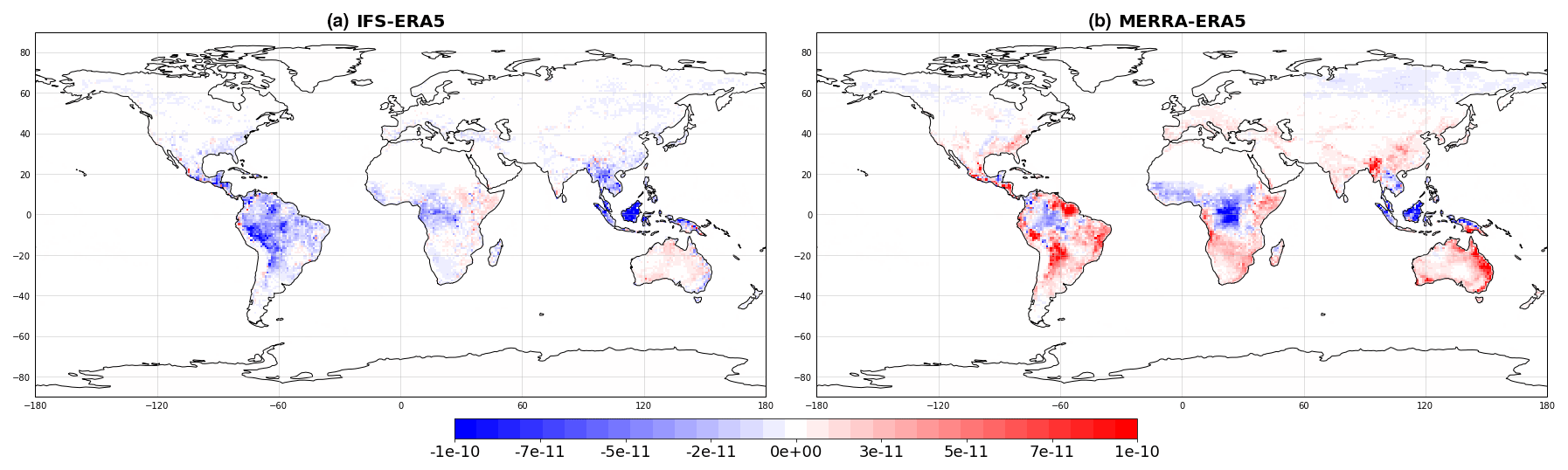
Figure 9 Annual mean isoprene difference (kg m⁻² s⁻¹) between S1-IFS and reference simulation (a) and between S1-MERRA and reference simulation (b).

As shown by Guenther et al. (2006), the estimate of isoprene flux in MEGAN is temperature dependent, with emissions increasing exponentially with temperature to a maximum that depends on the average temperature of the last 24 h. MEGAN emissions depend also on the amount of light received by vegetation. The isoprene estimate increases almost linearly with PPFD; the rate of increase depends on the average PPFD over the last 24 h. To study the linear dependence between the isoprene flux estimates and PPFD, we examined the correlation between the difference in isoprene estimates and the difference in light (PAR) between the reference (with the ERA5 meteorological forcing) and S1 simulations (with the IFS and MERRA meteorological forcings). Figure 10 displays the temporal correlation coefficient between isoprene flux differences and light differences for the reference and S1-IFS simulations, as well as for the reference and S1-MERRA simulations. The PAR contributes strongly to the explanation of isoprene discrepancies between the reference and S1 simulations, as the correlation coefficient exceeds 0.8 in regions where isoprene is emitted. Thus, the difference in isoprene emission flux across the three simulations is mainly due the different PAR input used in the simulation’s meteorological forcing file. The correlation study was not conducted on other isoprene meteorological drivers, such as temperature, as the dependence of isoprene on this parameter is exponential.

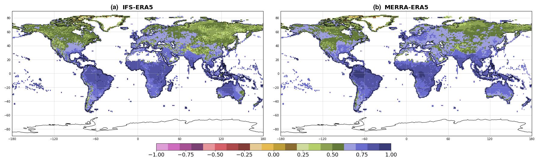
Figure 10 Pearson correlation coefficient of PAR and isoprene difference between reference and S1 simulations (S1-IFS (a) and S1-MERRA (b)).

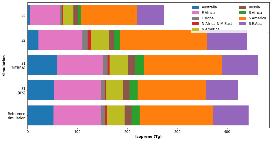
Figure 11 Isoprene total emission by region (defined in Fig. 8) of the reference simulation, S1 simulation (IFS/MERRA), S2 simulation (emission potential), and S3 simulation (soil moisture).

Figures 11 and 12 represent the isoprene distribution by region for all tests performed and the mean temperature/PAR relative difference between the MERRA and the ERA5 data inputs. On a regional scale, MERRA temperature and downward radiation received by vegetation are higher in Australia and South America compared to ERA5, resulting in higher isoprene estimates in those regions (+10 % in Australia and +7 % in South America). Conversely, MERRA temperature and radiation inputs are lower in East Africa, resulting in lower isoprene estimates for that region (−3 %).

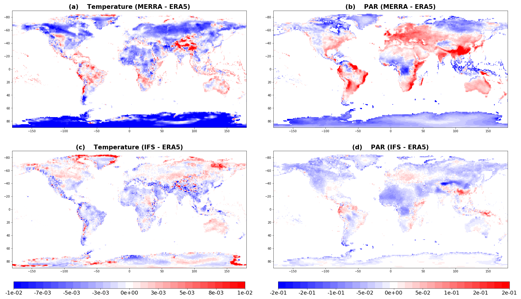
Figure 12 Mean temperature relative difference between MERRA and ERA5 (a), mean PAR relative difference between MERRA and ERA5 (b), mean temperature relative difference between IFS and ERA5 (c), and mean PAR relative difference between IFS and ERA5 (d). Red represents areas where the difference between temperature/PAR is positive, and blue represents areas where the difference is negative.

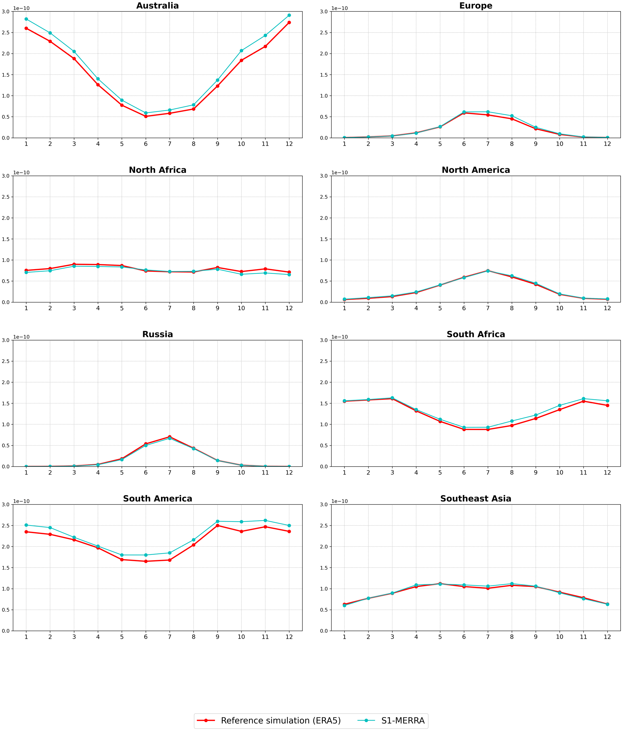
A regional analysis was also conducted to quantify the impact of using different meteorological datasets on isoprene estimates. Figure 13 displays the monthly isoprene emissions of the reference and S1-MERRA simulations across regions of the globe shown in Fig. 8. The isoprene flux absolute difference is mostly pronounced in Australia, South America, and Southern Africa, where S1-MERRA isoprene estimates are higher than the reference simulation. In South America, Southern Africa, and Australia, S1-MERRA monthly isoprene emissions are higher than the reference simulation by a range of 2 %–10 %, 1 %–11 %, and 6 %–15 %. In these regions, although the temperature difference between MERRA and ERA5 is small (less than 0.5°), the photosynthetically active radiation (PAR) difference is significant. In these regions, PAR variations range at −1–9, −2–8, and −1–8 W m⁻² respectively. Consequently, the main factor driving monthly variations in isoprene emissions between the reference simulation and the S1-MERRA simulation is PAR.

Several studies have been conducted to quantify the sensitivity of the MEGAN model to meteorology. For example, Arneth et al. (2011) showed that using different meteorological forcings can lead to different emission estimates where the use of CRU (Climatic Research Unit) meteorology instead of the NCEP (National Center for Environmental Prediction) reanalysis product led to a 10 % decrease with MEGANv2. Sindelarova et al. (2022) also detected a difference of the total BVOC MEGANv2.1 estimations between CAMS-GLOB-BIOv1.2 and CAMS-GLOB-BIOv3.1 and explained that the discrepancies are mainly due to the use of different meteorological inputs.

On a global scale, the use of different meteorological forcing has been found to have an impact on the amount of isoprene emissions estimated with the SURFEX–MEGAN model. The use of MERRA meteorology led to a 5 % increase in isoprene emissions, while the use of IFS meteorology resulted in a decrease of 4.8 % in comparison with the reference simulation.

Figure 13 Monthly variation in isoprene flux from the reference and S1-MERRA simulations of regions of the globe defined in Fig. 8 in kg m⁻² s⁻¹.

4.2 Emission potential of isoprene

MEGANv2.1 defines two approaches to estimate biogenic fluxes. The first one is based on the use of the biogenic species emission potential maps ϵ_map; these gridded maps are made based on a land cover including more than 2000 eco regions each with specific emission factors (Guenther et al., 2012). The compilation of these maps accounts for the large differences in emission potential between species belonging to the same generalized PFT (e.g. temperate deciduous tree). For other PFTs, including only low isoprene emitters, the use of the PFT-specific emission factor is sufficient (e.g. boreal deciduous and needle trees). The second approach consists of using the 16 generalized plant functional type distributions ϵ_PFT, along with their specific emission factor (Guenther et al., 2012).

To compare the two approaches, we estimated global isoprene fluxes during 2019 using emission potential values ϵ_PFT instead of the emission potential data from the gridded maps ϵ_map used in the reference simulation. Figure 14 shows the mean difference in isoprene emissions between the S2 simulation using ϵ_PFT and the reference simulation using ϵ_map. The total annual isoprene of simulation S2 is 390 Tg; the data indicate that on a global scale, the isoprene emissions have decreased by 12 %. As shown in Fig. 11, this decrease is particularly pronounced in Australia (−58 %) and Southern Africa (−25 %). A notable increase is observed in Europe (+32 %) and in South America (+19 %), particularly in the northern Amazon. The red dots over islands shown in Fig. 14 are due to the fact that the isoprene emission factor from the input emission potential map is equal to 0 in these areas.

The results of this sensitivity test are aligned with the findings of Sindelarova et al. (2014). The MEGAN-MACC average annual isoprene emissions dropped by 14 % when using the emission potential values ϵ_PFT instead of the emission potential map ϵ_map. The decrease concerns Australia (−47 %) and Southern Africa (−28 %) and the increase concerns South America (+10 %) and Europe (+18 %).

Figure 15 represents the annual mean isoprene flux obtained with the S2 sensitivity simulation. The results of this sensitivity test partially explain the differences observed in Sect. 3. CAMS-GLOB-BIOv3.0 and ALBERI inventories used ϵ_PFT data to estimate isoprene flux, resulting in lower isoprene emissions compared to other datasets, as annual isoprene flux dropped by 29 % and 21 % respectively compared to the reference simulation. Sindelarova et al. (2022) reported a similar decrease rate in isoprene emissions estimated at 30 % of CAMS-GLOB-BIOv3.0, which uses PFT-specific emission potential data and PFT distributions, compared to CAMS-GLOB-BIOv3.1, which uses isoprene emission potential gridded maps.

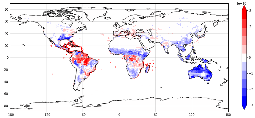
Figure 14 Annual mean isoprene difference (kg m⁻² s⁻¹) between sensitivity test S2 and the reference simulation.

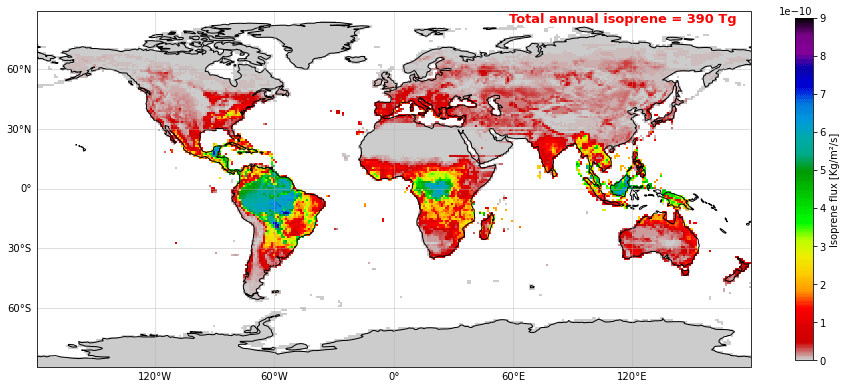
Figure 15 Annual mean isoprene flux (kg m⁻² s⁻¹) of S2 sensitivity simulation.

4.3 Soil moisture

Prior research has investigated the association between soil moisture and isoprene emissions. The results indicate that isoprene emissions exhibit a three-phased response to drought and declining soil water. In the initial days of drought, plants tend to retain a stable isoprene emission rate; in some instances, the emission rate may even slightly increase (Pegoraro et al., 2007). The second stage starts when soil moisture falls below a specific threshold, at which point the rate of isoprene emission begins to decrease. Extended exposure to severe drought leads to a gradual decrease in isoprene emissions; eventually, the emissions become insignificant over time (Tingey et al., 1981; Pegoraro et al., 2004b; Wang et al., 2021; Y. Wang et al., 2022; Trimmel et al., 2023).

The response of isoprene emission to drought is simulated in MEGAN indirectly via the MEGAN canopy environment model by incorporating the leaf temperature estimate, which is affected by soil moisture. MEGAN also includes a γ_SM factor which directly simulates the response of isoprene emissions to drought. This factor is derived from soil moisture parameterization experiments conducted by Pegoraro et al. (2004a). The γ_SM is defined as follows:

$$\begin{array}{}\text{(8)}& \begin{array}{rl}& {\mathit{\gamma }}_{\mathrm{SM}}=\mathrm{1}\mathit{\theta }>{\mathit{\theta }}_{\mathrm{1}}\\ & {\mathit{\gamma }}_{\mathrm{SM}}={\displaystyle \frac{(\mathit{\theta }-{\mathit{\theta }}_w)}{\mathrm{\Delta }{\mathit{\theta }}_{\mathrm{1}}}}{\mathit{\theta }}_w<\mathit{\theta }<{\mathit{\theta }}_{\mathrm{1}}\\ & {\mathit{\gamma }}_{\mathrm{SM}}=\mathrm{0}\mathit{\theta }<{\mathit{\theta }}_w,\end{array}\end{array}$$

where θ is the soil moisture (volumetric water content, m³ m⁻³), θ_w (m³ m⁻³) is the wilting point (the soil moisture level below which plants cannot absorb water from soil), Δθ₁ (= 0.04) is an empirical parameter, and θ₁ = θ_w + Δθ₁ (Guenther et al., 2012).

The third sensitivity test (S3) was conducted to examine the effect of soil moisture on isoprene emissions. To estimate γ_SM, MEGAN uses wilting point data calculated in SURFEX from the sand and clay covers given as input to the coupled model following the approaches by Clapp and Hornberger (1978) and Lepistö et al. (1988). The sand and clay data are extracted from HWSD (The Harmonised World Soil Database), which is a global soil database developed by the FAO (Food and Agriculture Organisation of the United Nations) in collaboration with IIASA (International Institute for Applied Systems Analysis) in order to provide information on the physical and chemical properties of soils across the world.

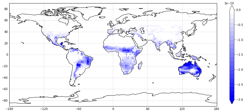
Figure 16 Annual mean isoprene difference (kg m⁻² s⁻¹) between sensitivity test S3 and the reference simulation.

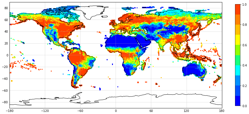
Figure 17 Spatial distribution of the annual mean soil moisture dependence factor γ_SM in the S3 simulation.

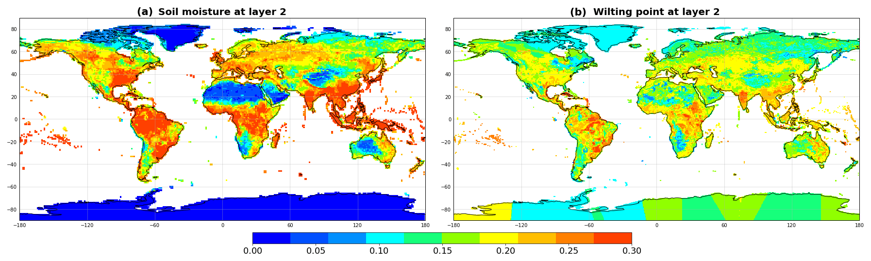
Figure 18 Annual average soil liquid water content (m³ m⁻³) (a) and wilting point data (m³ m⁻³) (b) of the ISBA-2L second layer.

In order to accurately estimate soil moisture, a 4-year spin-up period was required to stabilize the soil water content with the ISBA force-restore 2-L scheme. This approach is used to simulate the exchange of energy and water between the surface and the atmosphere and is based on the balance between the forces that drive the exchange of energy and water (radiation, temperature, and precipitation) and the restoring forces that return the system to equilibrium (evaporation, transpiration, and runoff) (Boone et al., 1999) (Hu and Islam, 1995). The wilting point and soil water content are calculated at different soil layers, depending on the ISBA scheme model used. In the ISBA force-restore 2-L scheme, the soil is represented with two layers. In the present study, to evaluate soil moisture impact on isoprene emissions, we used soil moisture and wilting point data from the second layer, as it most accurately represents the root depth of the vegetation.

The integration of the soil moisture algorithms led to total isoprene emissions of 273 Tg, with a global decrease of 38 % compared to the reference simulation. Figures 16, 17, and 18 show the annual mean isoprene difference between the S3 simulation and the reference simulation, the spatial distribution of average γ_SM over 2019, and the annual mean soil liquid water content estimated at the second ISBA-2L layer as well as the relative wilting point data used in the S3 simulation respectively. The decrease concerns mainly arid and semi-arid regions; the largest decrease can be observed in Australia (−89 %), followed by North Africa and the Middle East (−82 %), Southern Africa (−67 %), and East Africa (−38 %). In South America, emissions are lower by 23 % and the decrease is mainly located in Brazil. Previous studies have analysed the impact of soil moisture on isoprene emissions and have reported varying decrease rates. Guenther et al. (2006) obtained the lowest decrease rate of 7 %, Müller et al. (2008) found a decrease rate of 21 %, and Sindelarova et al. (2014) reported the highest decrease rate of 50 %. The discrepancies in the reported values of the decreased isoprene rate can be attributed to the use of different soil moisture and wilting point data. The latter is a critical parameter, as it defines the limit below which the soil moisture activity factor is set to 0; consequently, Guenther et al. (2012) stressed the importance of using consistent wilting point data with the soil moisture input. In this context, the SURFEX–MEGAN model enhances the precision of γ_SM calculations by using vegetation-type-dependent soil moisture at a given layer and wilting point data at the same soil layer.

Several limitations associated with the use of this MEGANv2.1 soil moisture parameterization have been identified. Primarily, the parameterization exhibits a significant dependency on the wilting point data, which can show inconsistency with the soil moisture data used. Furthermore, it has been shown that this parameterization substantially reduces isoprene emissions, even under moderate drought conditions, thereby indicating a potential over-sensitivity to drought stress (H. Wang et al., 2022). The introduction of the new MEGAN3 soil moisture factor addresses these shortcomings by providing robust performance under both moderate and severe drought conditions (Jiang et al., 2018). This enhancement in soil moisture representation is anticipated to be integrated into the forthcoming version of the SURFEX–MEGAN coupled model, thereby offering a more accurate and reliable prediction of isoprene emissions under varying soil moisture scenarios.

5 Conclusions

This paper describes the implementation of the biogenic model MEGANv2.1 (Guenther et al., 2012) in the surface model SURFEX (Le Moigne, 2018). The aim of this coupling is to improve the accuracy of vegetation-type-specific parameters for MEGAN2.1 by leveraging the detailed canopy environment model built into SURFEX. This improved accuracy should lead to better estimates of BVOCs.

The coupling evaluation was done by running a global simulation (1°, hourly) in 2019 using ERA5 meteorological data inputs. The total annual isoprene is estimated to be 443 Tg. The SURFEX–MEGAN total annual isoprene is within the range of isoprene estimates reported in previous studies. To evaluate the coupled model, the 2019 isoprene simulation results were compared with isoprene estimates of three previous published studies. A spatial and temporal analysis was conducted to compare the different results. The SURFEX–MEGAN emission estimates were shown to have a comparable spatial distribution to the other inventories, especially to those using a similar setup (e.g. meteorology, emission potential data). Regarding the monthly variation in isoprene emissions, SURFEX–MEGAN follows the same temporal pattern as some of the inventories; the shift in the annual isoprene cycle was explained by the difference in the contribution of the emitting regions to the global isoprene for each inventory.

A series of sensitivity tests were performed to investigate the impact of key MEGAN variables on isoprene emissions. To highlight the difference between the coupled SURFEX–MEGAN model and other MEGAN-based models, the results of the sensitivity tests were compared with the findings of other studies. The use of different meteorological forcings resulted in isoprene estimates varying by up to ±5 % of the reference run results, with Australia, South America, and Africa being the most affected regions. The use of different inputs of emission potential data led to a decrease of 12 % globally. The activation of the soil moisture parameterization was shown to have the greatest impact on isoprene emissions. On a global scale, the emission have decreased by 38 %, and the largest decrease was observed in Australia (−89 %) and in Africa. The decreased rate related to the activation of the soil moisture activity factor varies across different studies, which has been attributed to inconsistencies in the soil moisture and wilting point data employed. The SURFEX–MEGAN model offers an advantage in this regard, as it can compute the wilting point and soil moisture at the same soil layer for different vegetation types, leading to a more precise estimation of the gamma soil moisture. This high sensitivity to soil moisture emphasizes the importance of conducting further studies in this area in order to reduce uncertainties, in particular by refining the estimation of the empirical parameter Δθ₁.

The potential perspectives to be explored from this study concern the assessment of biogenic emissions in future climates, as BVOCs are expected to undergo significant changes resulting from the alteration of biogenic emission climate drivers. This assessment is particularly relevant to air quality forecasting in the context of ongoing global warming and predicted future climate change. In this respect, the particularity of SURFEX lies in its ability to be used in offline mode, as it can be forced with future climate meteorology. SURFEX also includes a biomass evolution sub-model, allowing for the evolution of vegetation density (leaf area index) as a function of changing meteorological and environmental variables. This feature would be of particular use for predicting biogenic emissions under future climate scenarios whereby the evolution in vegetation could be simulated in SURFEX using the dynamic LAI vegetation scheme.