Evaluation and development of surface layer scheme representation of temperature inversions over boreal forests in Arctic wintertime conditions

In this study, the Noah land surface model used in conjunction with the Mellor–Yamada–Janjić surface layer scheme (hereafter, Noah-MYJ) and the Noah multiphysics scheme (Noah-MP) from the Weather Research and Forecasting (WRF) 4.5.1 mesoscale model are evaluated with regard to their performance in reproducing positive temperature gradients over forested areas in the Arctic winter. First, simplified versions of the WRF schemes, recoded in Python, are compared with conceptual models of the surface layer in order to gain insight into the dependence of the temperature gradient on the wind speed at the top of the surface layer. It is shown that the WRF schemes place strong limits on the turbulent collapse, leading to lower surface temperature gradient at low wind speeds than in the conceptual models. We implemented modifications to the WRF schemes to correct this effect. The original and modified versions of Noah-MYJ and Noah-MP are then evaluated compared to long-term measurements at the Ameriflux Poker Flat Research Range, a forest site in interior Alaska. Noah-MP is found to perform better than Noah-MYJ because the former is a two-layer model which explicitly takes into account the effect of the forest canopy. Indeed, a non-negligible temperature gradient is maintained below the canopy at high wind speeds, leading to overall larger gradients than in the absence of vegetation. Furthermore, the modified versions are found to perform better than the original versions of each scheme because they better reproduce strong temperature gradients at low wind speeds.

1 Introduction

Surface-based temperature inversions (SBIs) are extremely frequent in the cold, dark conditions of the Arctic winter (Serreze et al., 1992; Bradley et al., 1992). The usual pattern is that cloudy conditions are associated with a near-neutral surface layer, while clear skies are associated with strong SBIs (Malingowski et al., 2014). However, modelling temperature inversions remains a challenge and an area of ongoing study (Steeneveld et al., 2006; Sterk et al., 2013; Holtslag et al., 2013; Baas et al., 2017).

One of the main difficulties is with modelling the turbulent heat fluxes. Typical Monin–Obukhov stability theory (MOST) assumes constant fluxes in the surface layer and so-called z-less scaling (Monin and Obukhov, 1954; Wyngaard and Coté, 1972), and its limits of applicability have been discussed (Grachev et al., 2008). This has led to the recognition of different turbulent regimes. The first, called the weakly stable regime, is fully consistent with MOST. In this regime, the turbulent heat fluxes increase with increasing temperature gradient because more heat is available to be transported. The inertial range in the turbulence spectra is well defined and exhibits a Kolmogorov slope of $-\mathrm{5}/\mathrm{3}$ (Kaimal and Finnigan, 1994). The other is the strongly stable regime, where turbulent sensible heat fluxes instead decrease with increasing temperature gradient because the effect of strong stability leads to a turbulence decay. In this regime, Kolmogorov turbulence becomes intermittent and driven by processes at larger timescales, such as the Coriolis force (Grachev et al., 2008) or gravity waves (Sorbjan and Czerwinska, 2013). However, it does not disappear entirely so that the flow never becomes laminar (Grachev et al., 2013).

There is general agreement on the nature of these two turbulence regimes (although sometimes a third “transitional” regime is considered). However, the separation between the two is debated: traditionally, the Richardson number (R_i) or Monin–Obukhov parameter (ζ) is used. Grachev et al. (2013), for example, suggested that a gradient or flux Richardson number of R_i=0.2 was a lower threshold for the strongly stable state, while Mahrt et al. (2014) found that ζ=0.06 separated the two states. More recent works have focused on the impact of wind speeds, or wind shear, on determining the regime (Sun et al., 2012; van de Wiel et al., 2007; van de Wiel et al., 2012) in a framework called minimum wind speed for sustainable turbulence (MWST). For example, van Hooijdonk et al. (2015), building on the work of van de Wiel et al. (2012), used external forcings to the surface layer (such as a constant wind speed, replacing the synoptic pressure gradient and downwards radiative fluxes) to determine a new parameter called the shear capacity. This parameter has been found to better predict the stability regime than the traditional local parameters such as ζ or R_i. In this new framework, the stability regime is not solely a feature of the turbulence but of the surface layer as a whole.

Determining the stability regime and the turbulent heat fluxes is, however, only one part of determining the SBI strength. This depends on the surface temperature, which is in turn determined by the surface energy budget (SEB). Analysis of measurements in the Antarctic has shown that plotting ΔT (the temperature difference between the surface and 10 m) versus the wind speed at 10 m under clear-sky winter conditions reveals two distinct regimes, separated by a transition: one at low wind speeds and high ΔT and the other at high wind speeds and low ΔT (Vignon et al., 2017). This characteristic shape was termed the “S” shape (although the S is technically backwards) because the transition exhibited some non-monotonous behaviour. The transition between the two regimes was found to agree well with predictions from MWST. Drawing on these studies, a small analytical model was developed by van de Wiel et al. (2017) and was shown to reproduce the “S” shape.

MWST therefore offers a promising framework for the analysis and modelling of SBIs. For the moment, however, these analyses have been restricted to the extreme conditions of Antarctica, where the surface is vegetation-free snow and ice. The Arctic and sub-Arctic also experience regular inversions with strong implications for pollution dispersion. However, a large part of this region is covered by forest, which is known to impact the turbulent heat fluxes (Batchvarova et al., 2001). For example, unstable stratification may remain within the canopy layer even when the overlying air layer is very stable (Jacobs et al., 1992), and gradients directly above the canopy may be modified by the roughness sublayer (Mölder et al., 1999; Babić et al., 2016). Forest canopies also act as grey bodies, both emitting and absorbing long-wave fluxes. In seeking to extend the use of MWST, it is therefore important to consider the impact of trees. Another important question concerns the coherence of mesoscale models with MWST. Vignon et al. (2018), for example, showed that the Laboratoire de Météorologie Dynamique – Zoom (LMDZ) model reproduced an S-shaped transition of surface temperature gradient with wind speed, with the shape of the transition depending on the stability function used. This represents a promising new framework for improving the representation of surface layer temperature inversions.

This paper therefore has two coupled aims. The first is to investigate the impact of wind speed on the temperature gradient in clear-sky, winter conditions over a forest surface using a multiyear observational dataset from a forest of interior Alaska. The second is to evaluate and improve the performance of Weather Research and Forecasting (WRF) model schemes in representing the temperature gradient at this forest site. Here, the parts of the WRF code responsible for calculating the surface temperature gradient are referred to as the Surface Energy Budget and Surface Layer (SEB-SL) model because they calculate the turbulent energy exchanges in the surface layer and solve the surface energy budget. In WRF, the SEB-SL model is often split into two parts: the surface layer scheme and the land surface model. In Sect. 2, conceptual SEB-SL models are introduced and used to gain insight into the development of temperature inversions and shed light on two different WRF SEB-SL schemes. In Sect. 3, the measurements from the Ameriflux Poker Flat Research Range near Fairbanks, Alaska, are presented. In Sect. 4, two WRF SEB-SL schemes are presented, and modifications are proposed. Lastly, the behaviour of the two original WRF schemes and their modified versions is compared based on the Ameriflux measurements (Sect. 5).

2 Conceptual models of the surface layer

In this section, conceptual models of the surface layer are presented (Sect. 2.1). These models are used to gain insight into the impact of different variables (and, especially, of the wind speed) on the resulting surface–air temperature gradient in order to help with the analysis of the WRF surface layer schemes.

2.1 Model presentation

A single-layer conceptual SEB-SL model was developed by van de Wiel et al. (2017) to study the impact of the wind speed on the near-surface temperature gradient. In the presence of trees or other tall vegetation, however, the introduction of a second layer becomes necessary. Here, such a model is developed. It is composed of the surface, a “canopy” layer where the air is in thermodynamic equilibrium with the vegetation, and an overlying air layer (Fig. 1). The effects of the canopy on the long-wave radiative and turbulent fluxes are then taken into account. In the following, the equations and notations draw on the one-layer model of van de Wiel et al. (2017). The surface emissivity is assumed to be equal to 1, which is a good approximation for snow-covered surfaces. The short-wave radiation and the latent heat fluxes are neglected in Arctic wintertime conditions.

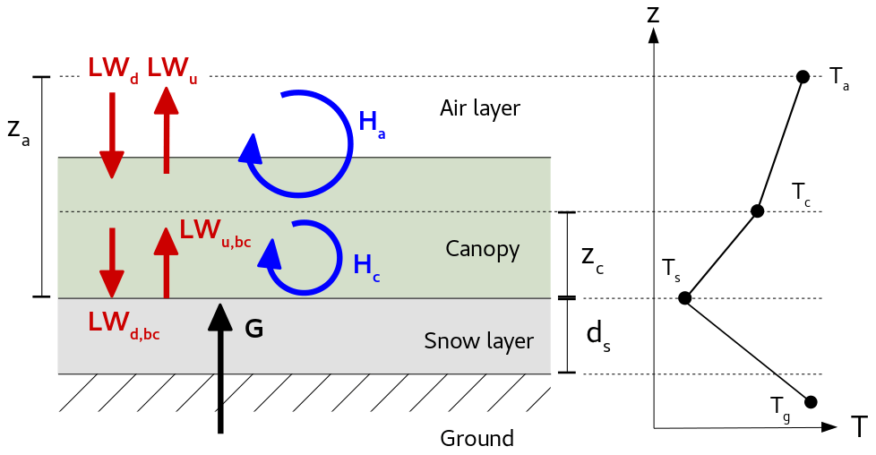
Figure 1 Schematic of the two-layer model described in this section. LW_d and LW_u are the downwards and upwards long-wave fluxes above the canopy, and LW_d,bc and LW_u,bc are the downwards and upwards long-wave fluxes below the canopy. H_a is the turbulent sensible heat flux between the canopy and overlying air. H_c is the turbulent sensible heat flux between the canopy and surface. G is the conduction flux through the snow.

The surface energy balance equation in this system can be written as (Appendix A)

$$\begin{array}{}\text{(1)}& \begin{array}{rl}-(\mathrm{1}-{\mathit{ϵ}}_{\mathrm{c}})Q_{\mathrm{i}}-{\mathrm{\Lambda }}_{\mathrm{s}}(T_{\mathrm{a}}-T_{\mathrm{g}})& +\mathrm{\Delta }{T}_{\mathrm{cs}}\left[\mathit{\rho }{C}_p{C}_{\mathrm{D},\mathrm{c}}{U}_{\mathrm{c}}+\mathrm{4}\mathit{\sigma }{T}_{\mathrm{a}}^{\mathrm{3}}+{\mathrm{\Lambda }}_{\mathrm{s}}\right]\\ & +\mathrm{\Delta }{T}_{\mathrm{ac}}\left[(\mathrm{1}-{\mathit{ϵ}}_{\mathrm{c}})\mathrm{4}\mathit{\sigma }{T}_{\mathrm{a}}^{\mathrm{3}}+{\mathrm{\Lambda }}_{\mathrm{s}}\right]\\ & =\mathrm{0},\end{array}\end{array}$$

where $\mathrm{\Delta }{T}_{\mathrm{cs}}=T_{\mathrm{c}}-T_{\mathrm{s}}$ is the difference between the surface temperature (T_s) and the air temperature at canopy height (T_c). $\mathrm{\Delta }{T}_{\mathrm{ac}}=T_{\mathrm{a}}-T_{\mathrm{c}}$ is the difference between the canopy temperature and the air temperature at height z_a, corresponding to the top of the surface layer (T_a). T_g is the ground temperature (Fig. 1). $Q_{\mathrm{i}}=-{\text{LW}}_{\mathrm{d}}+\mathit{\sigma }{T}_{\mathrm{a}}^{\mathrm{4}}$ (where LW_d is the downwards long-wave flux) is termed the isothermal net radiation: indeed, it is equal to the net long-wave flux if T_s=T_a (Holtslag and Bruin, 1988). ${\mathrm{\Lambda }}_{\mathrm{s}}=\frac{{\mathit{\lambda }}_{\mathrm{s}}}{d_{\mathrm{s}}}$, where λ_s is the snow conductivity and d_s the snow depth. ρ is the air density, C_p the heat capacity of the air and U_c the wind speed at height z_c. For the time being, U_c is very roughly estimated to be proportional to U_a: for example, $U_{\mathrm{c}}=\mathrm{0.25}\cdot U_{\mathrm{a}}$. ϵ_c is the canopy emissivity, and C_D,c is the turbulent diffusion coefficient for the canopy-to-surface heat exchange.

A second equation can be obtained by considering the canopy energy balance (Appendix A):

$$\begin{array}{}\text{(2)}& \begin{array}{rl}-Q_{\mathrm{i}}-{\mathrm{\Lambda }}_{\mathrm{s}}(T_{\mathrm{a}}-T_{\mathrm{g}})& +\mathrm{\Delta }{T}_{\mathrm{cs}}\left[(\mathrm{1}-{\mathit{ϵ}}_{\mathrm{c}})\mathrm{4}\mathit{\sigma }{T}_{\mathrm{a}}^{\mathrm{3}}+{\mathrm{\Lambda }}_{\mathrm{s}}\right]\\ & +\mathrm{\Delta }{T}_{\mathrm{ac}}\left[\mathrm{4}\mathit{\sigma }{T}_{\mathrm{a}}^{\mathrm{3}}+{\mathrm{\Lambda }}_{\mathrm{s}}+\mathit{\rho }{C}_p{C}_{\mathrm{D},\mathrm{a}}{U}_{\mathrm{a}}\right]\\ & =\mathrm{0},\end{array}\end{array}$$

where U_a is the wind speed at height z_a, and C_D,a is the turbulent diffusion coefficient for the air–canopy heat exchange. This is very similar to the one-layer model of van de Wiel et al. (2012), except that the energy source term (here, the first line of Eq. 2) has an additional term, which is proportional to ΔT_cs. The difficulty in solving Eqs. (1) and (2) to obtain ΔT_cs and ΔT_ac is that the turbulent diffusion coefficients depend on the stability:

$$\begin{array}{ll}{\displaystyle }{C}_{\mathrm{D},\mathrm{c}}& {\displaystyle }={\displaystyle \frac{{\mathit{\kappa }}^{\mathrm{2}}}{\left[\log \right(\frac{z_{\mathrm{a}}}{z_{\mathrm{0}\mathrm{s}}})-\mathit{\psi }(\mathit{\zeta })+\mathit{\psi }(\frac{z_{\mathrm{0}\mathrm{s}}}{L}){]}^{\mathrm{2}}}}\\ \text{(3)}& {\displaystyle }{C}_{\mathrm{D},\mathrm{a}}& {\displaystyle }={\displaystyle \frac{{\mathit{\kappa }}^{\mathrm{2}}}{\left[\log \right(\frac{z_{\mathrm{a}}-d}{z_{\mathrm{0}\mathrm{c}}})-\mathit{\psi }(\mathit{\zeta })+\mathit{\psi }(\frac{z_{\mathrm{0}\mathrm{c}}}{L}){]}^{\mathrm{2}}}},\end{array}$$

where κ=0.4 is the van Kármán constant, and z_0s and z_0c are the roughness lengths of snow or of the canopy, respectively. Here, d is the displacement height due to the presence of the canopy. The snow and canopy momentum roughness length $z_{\mathrm{0}\mathrm{m},\mathrm{s}/\mathrm{c}}$ is assumed to be equal to the heat roughness length $z_{\mathrm{0}\mathrm{h},\mathrm{s}/\mathrm{c}}$, both referred to as $z_{\mathrm{0},\mathrm{s}/\mathrm{c}}$. $\mathit{\zeta }=z/L$ is the Obukhov parameter, with L being the Monin–Obukhov length. ψ is the integral stability function, which tends to 0 when ζ≈0 and tends to infinity with increasing ζ. The turbulent diffusion coefficients therefore tend to ${\mathit{\kappa }}^{\mathrm{2}}/\log (\frac{z}{z_{\mathrm{0}}}{)}^{\mathrm{2}}$ at weak stability and 0 at strong stability. Many different expressions of ψ are found in the literature (Businger et al., 1971; Holtslag and Bruin, 1988). Usually, these are classified as “short tail” (i.e. with a very sharp decrease so that C_D quickly drops to 0 at increasing stability) or “long tail” (i.e. the transition is smoother so that some turbulent sensible heat flux is maintained for longer). There are also other ways to estimate the below-canopy turbulent diffusion coefficient C_D,c, for example by assuming an exponential wind profile in the canopy as in Mahat et al. (2013). However, Eq. (3) is the simplest expression and is utilised for illustrative purposes.

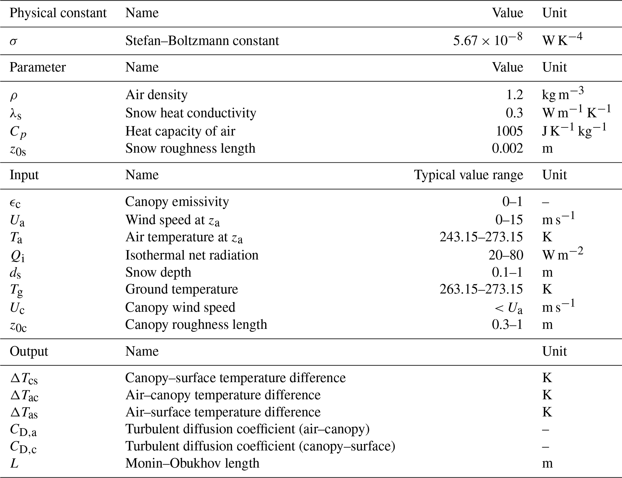
Table 1 List of the constants, parameters and variables (both input and output) used in the conceptual model. For the inputs, a typical range of values for the Arctic winter (in clear-sky conditions) is indicated.

2.2 Weakly and strongly stable limits

The first insights into the behaviour of ΔT_cs and ΔT_ac can be gained by studying the asymptotic cases: the weakly and strongly stable limits, defined by U_a→∞ and U_a→0, respectively, while keeping ΔT_as>0. Here only the case where ϵ_c=1 (corresponding to an opaque canopy) is considered. In this situation, and if turbulence is completely collapsed (i.e. $C_{\mathrm{D},\mathrm{a}}=C_{\mathrm{D},\mathrm{c}}=\mathrm{0}$), Eqs. (1) and (2) lead to the following values for the temperature gradients:

$$\begin{array}{ll}{\displaystyle }\mathrm{\Delta }{T}_{\mathrm{ac}}& {\displaystyle }={\displaystyle \frac{Q_{\mathrm{i}}\left[\mathrm{1}+{\mathrm{\Lambda }}_{\mathrm{s}}/\left(\mathrm{4}\mathit{\sigma }{T}_{\mathrm{a}}^{\mathrm{3}}\right)\right]+{\mathrm{\Lambda }}_{\mathrm{s}}(T_{\mathrm{a}}-T_{\mathrm{g}})}{\mathrm{4}\mathit{\sigma }{T}_{\mathrm{a}}^{\mathrm{3}}+\mathrm{2}{\mathrm{\Lambda }}_{\mathrm{s}}}}\\ \text{(4)}& {\displaystyle }\mathrm{\Delta }{T}_{\mathrm{cs}}& {\displaystyle }={\displaystyle \frac{-{\mathrm{\Lambda }}_{\mathrm{s}}{Q}_{\mathrm{i}}/\left(\mathrm{4}\mathit{\sigma }{T}_{\mathrm{a}}^{\mathrm{3}}\right)+{\mathrm{\Lambda }}_{\mathrm{s}}(T_{\mathrm{a}}-T_{\mathrm{g}})}{\mathrm{4}\mathit{\sigma }{T}_{\mathrm{a}}^{\mathrm{3}}+\mathrm{2}{\mathrm{\Lambda }}_{\mathrm{s}}}},\end{array}$$

and therefore,

$$\begin{array}{}\text{(5)}& \mathrm{\Delta }{T}_{\mathrm{as}}=\mathrm{\Delta }{T}_{\mathrm{ac}}+\mathrm{\Delta }{T}_{\mathrm{cs}}={\displaystyle \frac{Q_{\mathrm{i}}+\mathrm{2}{\mathrm{\Lambda }}_{\mathrm{s}}(T_{\mathrm{a}}-T_{\mathrm{g}})}{\mathrm{4}\mathit{\sigma }{T}_{\mathrm{a}}^{\mathrm{3}}+\mathrm{2}{\mathrm{\Lambda }}_{\mathrm{s}}}}.\end{array}$$

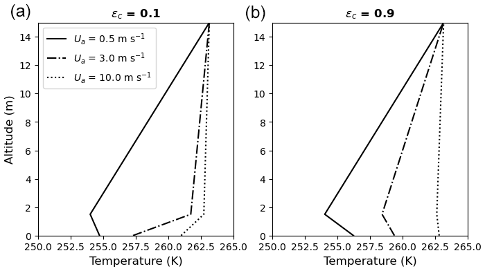
Figure 2 Profile calculated by the theoretical model for Q_i=50 W m⁻², $T_{\mathrm{a}}=-\mathrm{10}$ °C, $T_{\mathrm{g}}=-\mathrm{2}$ °C and Λ_s=1 W m⁻² K⁻¹, for three values of the wind speed U_a (0.5, 3 and 10 m s⁻¹). The turbulence was solved iteratively using the Ameriflux stability function. The only difference between the two graphs is the canopy emissivity: (a) ϵ_c=0.1 and (b) ϵ_c=0.9.

The total temperature gradient ΔT_as (between the air and the surface) in Eq. (5) is very similar to the one-layer case but with an “equivalent snow conductivity” that is twice the real value.

It can also be noted that ΔT_ac will usually be positive for typical Arctic winter values of the different parameters (Table 1) because radiation is the dominant process, unless the snow cover is very thin. For example, in a very cold, high-synoptic-pressure situation with Q_i=70 W m⁻², $T_{\mathrm{a}}=-\mathrm{20}$ °C and T_g=0 °C, ΔT_ac will be positive unless the snow depth is less than 7 cm. Similarly, in a warmer, cloudier situation with Q_i=30 W m⁻², $T_{\mathrm{a}}=-\mathrm{10}$ °C and T_g=0 °C, ΔT_ac will be positive unless the snow depth is less than 8 cm. For the same reason, ΔT_cs will usually be negative. In short, the very stable case is characterised by a temperature decrease from the surface to the canopy and an increase from the canopy to the overlying air. This is illustrated in Fig. 2 (continuous line, corresponding to U_a=0.5 m s⁻¹).

This is contradictory to the idea that C_D,c collapses to 0 because in the presence of a negative temperature gradient, buoyancy effects may generate turbulence without significant mechanical shear. Indeed, solving Eqs. (1) and (2) numerically for $U_{\mathrm{c}}=U_{\mathrm{a}}=\mathrm{0.001}$ m s⁻¹ (using appropriate schemes for calculating the turbulent diffusion coefficients such as those described in Sect. 4.1.1) shows that C_D,cU_c maintains a value of around 0.0017 m s⁻¹. Therefore, while the surface layer as a whole may be considered strongly stable (because T_a−T_s is very large), this may not be the case for the canopy layer. This is in agreement with Batchvarova et al. (2001), who found that the canopy layer may remain unstable even when the air aloft is very stably stratified.

2.3 Transition between the weakly and strongly stable limits

Next, the turbulence is solved iteratively using the Ameriflux stability function (Sect. 3.2) over a complete range of U_a values. This makes it possible to study the behaviour of the inversion outside of the weakly and strongly stable regimes and for different values of the canopy emissivity. The result of this estimation is shown in Fig. 3a, b for three values of ϵ_c. ΔT_ac exhibits the same S shape as in the one-layer conceptual model of van de Wiel et al. (2017). On the other hand, ΔT_cs is larger in the weakly stable regime than in the strongly stable regime (where it is negative, in coherence with the above discussion), and its shape is more dependent on values of the canopy emissivity. For ϵ_c=1, ΔT_cs appears to tend to 0 at large values of U_a while keeping negative values. On the other hand, for ϵ_c=0.5 and 0.1, it turns positive before decreasing with increasing wind speeds, therefore reaching a maximum somewhere between 2 and 6 m s⁻¹. In sum, the total temperature difference (ΔT_as) decreases more slowly than in the one-layer model, even when accounting for the long-tailed function chosen. The transition between the two modes (weak winds associated with strong inversions and high winds associated with weak inversions) is much more gradual in this two-layer conceptual model than the characteristic marked inverted S shape reported in the one-layer conceptual model of van de Wiel et al. (2017). This phenomenon corresponds to observations over a surface covered by trees that attenuate the transition.

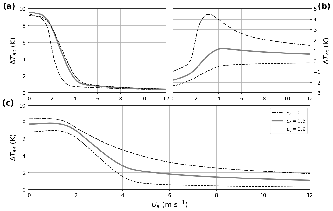
Figure 3 (a) ΔT_ac as a function U_a, as calculated by the conceptual model. The different line styles correspond to different values of the canopy emissivity. The transition between the two regimes has been calculated using the MYJ algorithm (Sect. 4.1.1) with the Ameriflux stability function (Sect. 3.2). All curves have been calculated using Q_i=50 W m⁻², $T_{\mathrm{a}}=-\mathrm{10}$ °C, $T_{\mathrm{g}}=-\mathrm{2}$ °C and Λ_s=1 W m⁻² K⁻¹. (b), (c) The same as (a) but for ΔT_cs and ΔT_as, respectively.

This behaviour can be understood in the following way. At low wind speeds, the dominant process influencing the canopy layer is radiation: it emits more than it receives and therefore loses its heat to both the surface and the air above. As a result, it is colder than both. Although some turbulence remains due to buoyancy, this is not enough to compensate for the radiative heat loss. At high wind speeds, on the other hand, the whole SL is well mixed. Turbulence is the dominant process, linking the canopy layer to both the surface and the air above and maintaining their temperatures closely.

Starting from the strongly stable state, a small increase in wind speed will lead to increased turbulence mixing and a positive heat flow from the air above to the canopy. The canopy temperature will therefore increase. If the canopy has a strong emissivity, this increase in temperature will lead to increased radiation downwards to the surface and a corresponding increase in surface temperature. The canopy and surface will therefore warm at relatively the same pace (Fig. 2, right). On the other hand, if the emissivity of the canopy is low, it will not as easily convert its increased temperature into radiation. Its temperature will therefore increase rapidly without contributing to warming the surface, leading to a high ΔT_cs (Fig. 2, left). As the wind speed continues to increase, the canopy temperature will eventually be more or less equal to the temperature of the air above, and the surface continues to warm, thus leading to a decrease in ΔT_cs.

3 Measurements at the Ameriflux Poker Flat Research Range

The measurements at the Ameriflux Poker Flat Research Range were used to evaluate the behaviour of the WRF surface layer schemes and the suggested modifications. In this section, they are presented, and a first analysis of the link between wind speed and temperature gradient is put forward.

3.1 Site description

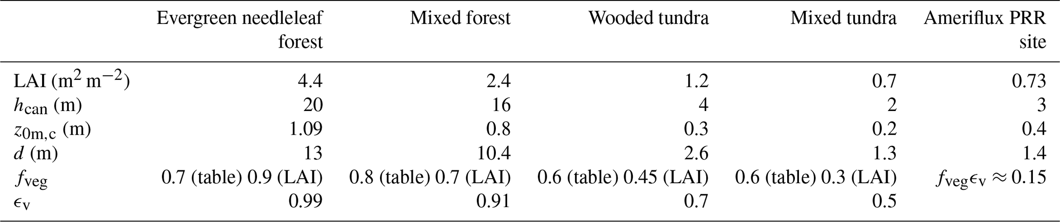
The Ameriflux PRR site is located in the Poker Flat Research Range (65°07^′24.4^′′ N, 147°29^′15.2^′′ W), around 30 km away from Fairbanks (interior Alaska). It has been operating since 2010, when it was established as part of the JAMSTEC-IARC Collaboration Study (JICS) (Sugiura et al., 2011), and its data are made available online on the Ameriflux website (Kobayashi et al., 2019) (https://ameriflux.lbl.gov/sites/siteinfo/US-Prr, last access: 22 April 2024). Its 17 m measurement tower is implanted in a black spruce forest with sparsely distributed and short trees (Fig. 4). The tree density, as measured in 2010, was 3967 trees ha⁻¹, and the average tree height was 2.44 m: the tallest tree was 6.4 m, but 75 % of trees were shorter than 3 m (Nakai et al., 2013). The leaf area index (LAI) was 0.73 (Nakai et al., 2013). Both of these values are much smaller than those found in Noah-MP for evergreen forests (Table 3).

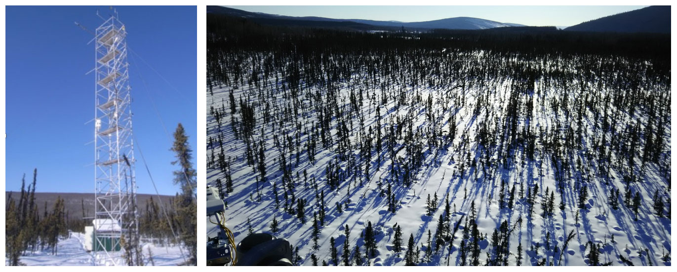
Figure 4 Left: photo of the 17 m high measurement tower at the Poker Flat Research Range at the Ameriflux site. Right: photo of the PRR site as seen from the measurement tower. Credit: Lisa Johnson.

Table 2 Meteorological variables measured at the Ameriflux PRR site, including instruments and measurement heights (Nakai et al., 2013). Note that wind speed is also measured at 11 m, with the sonic anemometer. Nakai et al. (2013) indicate that temperature was also measured at 7.5 m, but these measurements do not appear to be available on the Ameriflux website.

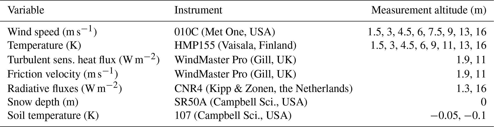
The Ameriflux PRR measurements that are used here are summarised in Table 2. These include wind speeds and temperatures at eight different heights (from 1.5 to 16 m), as well as turbulent and radiative fluxes. The surface temperature was calculated from the radiative flux measurements at 1.3 m, assuming a snow surface emissivity of 0.99. As this study focuses on the clear-sky surface layer in wintertime conditions, the data were curated accordingly. Only time points in the months of November–March with snow depth greater than 10 cm were kept. As no measurements of the cloud cover are available at the PRR site, clear-sky instants were defined as those with net long-wave radiation less than −30 W m⁻². Indeed, as is typical in high-latitude sites, the net long-wave flux (R_n) distribution at the PRR site was bimodal; the low-R_n mode was considered to correspond to the absence of clouds and the high-R_n mode to their presence. As the PRR site is located slightly below the Arctic circle, there is still some solar radiation at the surface in the wintertime. In order to simplify the analysis, only time points with downwelling short-wave radiation of less than 30 W m⁻² were kept; as the snow albedo is very high, this corresponds to a net short-wave flux of less than 5 W m⁻² and therefore to negligible short-wave impact. Lastly, measurements with a latent heat flux greater than 5 W m⁻² in absolute value were discarded.

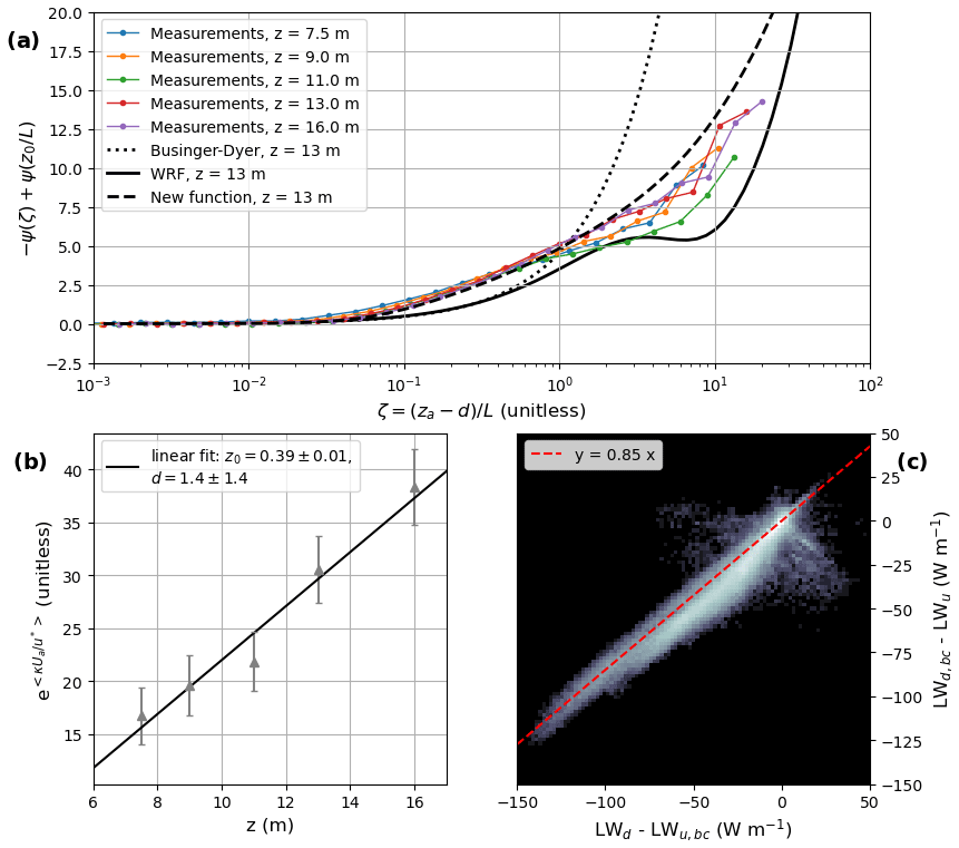
Figure 5 (a) Momentum integral stability function as a function of ζ determined from the PRR site measurement (coloured lines) and calculated using the Businger–Dyer and WRF formulations (black lines). The dashed line corresponds to the newly determined function for ψ (Eq. 7). (b) Determination of the PRR site above-canopy momentum roughness length and displacement height. (c) 2D histogram of ${\text{LW}}_{\mathrm{d},\mathrm{bc}}-{\text{LW}}_{\mathrm{u}}$ vs. ${\text{LW}}_{\mathrm{d}}-{\text{LW}}_{\mathrm{u},\mathrm{bc}}$. The red line corresponds to y=0.85x, yielding a canopy emissivity of 0.15.

3.2 PRR stability function

The average emissivity of the canopy layer ϵ_c=f_vegϵ_v can be calculated from above- and below-canopy radiation measurements:

$$\begin{array}{}\text{(6)}& {\text{LW}}_{\mathrm{d},\mathrm{bc}}-{\text{LW}}_{\mathrm{u}}=(\mathrm{1}-f_{\mathrm{veg}}{\mathit{ϵ}}_{\mathrm{v}})\left[{\text{LW}}_{\mathrm{d}}-{\text{LW}}_{\mathrm{u},\mathrm{bc}}\right].\end{array}$$

As shown in Fig. 5c, this gives a best estimation of ϵ_c≈0.15. This is in accordance with the Noah-MP calculation of f_veg and ϵ_v as a function of LAI. Indeed, measured LAI at the PRR site is 0.73, yielding f_veg≈0.3 (Eq. 12) and ϵ_v≈0.5.

The value of z_0m,c can also be calculated from the sonic anemometer data. Indeed, at weak stability (ζ≪1), the wind profile is approximately logarithmic:

$$U_{\mathrm{a}}\approx {\displaystyle \frac{u^{*}}{\mathit{\kappa }}}\log \left({\displaystyle \frac{z-d}{z_{\mathrm{0}\mathrm{m},\mathrm{c}}}}\right).$$

Therefore, d and z_0m,c can be determined through a linear regression of $e^{\mathit{\kappa }{U}_{\mathrm{a}}/u^{*}}$ against z when the data are restricted to values of $\mathit{\zeta }<{\mathrm{10}}^{-\mathrm{2}}$. Here, z_0m,c was found to be 0.39 m with $d=\mathrm{1.4}\pm \mathrm{1.4}$ m (Fig. 5b), which makes sense for a forest environment with short trees. The integral stability function ψ can also be determined from the data (assuming, as is often done, that it is the same for momentum and heat). The aim of this determination is to reproduce the measurements over the zone of transition, which is approximately between ζ=0.1 and ζ=1. For higher values (i.e. $z/L>\mathrm{3}$), the specific values of ψ are less problematic because in this range the turbulent heat flux will tend to collapse anyway. In order to determine ψ,

$$\mathrm{\Psi }=-\mathit{\psi }\left(\mathit{\zeta }\right)+\mathit{\psi }\left({\displaystyle \frac{z_{\mathrm{0}\mathrm{m},\mathrm{c}}}{L}}\right)={\displaystyle \frac{U_{\mathrm{a}}}{u^{*}}}\mathit{\kappa }-\log \left({\displaystyle \frac{z-d}{z_{\mathrm{0}\mathrm{m},\mathrm{c}}}}\right)$$

is plotted as a function of ζ (Fig. 5a). Because $z_{\mathrm{0}\mathrm{m},\mathrm{c}}/L$ is negligible compared to ζ, Ψ is approximately equal to −ψ(ζ) at the first order. Here, we found that measured ψ is more long tailed than the Businger–Dyer (Businger et al., 1971) or WRF (Eq. 9) functions. The intermediate zone (ζ between 0.1 and 1) exhibits a marked difference between the Businger-Dyer and WRF functions and the measurements. In fact, when plotted on a log–log scale, it became apparent that Ψ was proportional to $\sqrt{\mathit{\zeta }}$ at low values of ζ and proportional to ζ² at high values of ζ. This differs from the often-used z-less scaling, which implies that ψ must be proportional to ζ at least up to ζ≈0.1 (Monin and Obukhov, 1954; Grachev et al., 2013) as is the case for the WRF and Businger–Dyer functions. Measurement error may explain some of the difference at ζ<0.1 as Ψ is very small in these conditions.

For our purposes, we determined an analytical expression of ψ to best fit to the Ψ measurements and left aside the question of the z-less scaling. The following expression for ψ was therefore considered:

$$\begin{array}{ll}{\displaystyle }\mathit{\psi }\left(\mathit{\zeta }\right)& {\displaystyle }=-a\cdot {\mathit{\zeta }}^{r\left(\mathit{\zeta }\right)}\\ \text{(7)}& {\displaystyle }r\left(\mathit{\zeta }\right)& {\displaystyle }=\mathrm{0.75}\cdot \arctan (b\cdot \mathit{\zeta }-c){\displaystyle \frac{\mathrm{2}}{\mathit{\pi }}}+\mathrm{1.25}.\end{array}$$

This was chosen because arctan (x) tends to $\pm \frac{\mathit{\pi }}{\mathrm{2}}$ when x tends to ±∞, with a smooth transition around x=0. r(ζ), which therefore tends to 0.5 at low values of ζ and 2 at high values of ζ, similar to observations. The b and c coefficients must be chosen so that the timing and speed of the transition between the $\sqrt{\mathit{\zeta }}$ and ζ² asymptotes match the observations. The function Ψ was therefore fitted for the different heights (z=7.5, 9, 11, 13 and 16 m), yielding coefficients which varied between the ranges [4.5,5.5], $[-\mathrm{1},\mathrm{2}]$ and [10,40] for a, b and c, respectively. Plotting the function with these different parameters revealed little difference in behaviour over this range. Values of a=5, b=20 and c=0.1 were found to give a good fit to the observations (Fig. 5a). This expression of ψ was termed the PRR stability function.

The Ameriflux PRR site characteristics are summarised in Table 3. Although the location of the PRR site is given as evergreen needleleaf forest by the MODerate resolution Imaging Spectroradiometer (MODIS) land use categories as well as by the Ameriflux website, its canopy height and turbulent and radiative characteristics are actually the most similar to a wooded or mixed tundra.

3.3 Link between temperature gradients and wind speed at the Ameriflux PRR site

The average temperature profile (and its difference from the temperature at 16 m) is shown in Fig. 6a. The impact of wind speed on the surface layer temperature profile is clear. To highlight the importance of the wind speed on the regime stability, data are gathered in two groups according to their wind speed values: U_a< 2 m s⁻¹ or U_a> 4 m s⁻¹. This distinction is only used in Fig. 6 for illustrative purpose. This separation is based on the distribution of the bulk Richardson number R_b at 16 m (Fig. 6b): 65 % of the data with U_a>4 m s⁻¹ indeed have an R_b≤0.25, and 99.2 % of the data with U_a<2 m s⁻¹ have an R_b>0.25. The two modes are therefore clearly separated with a negligible overlap.

Figure 6 (a) Average temperature difference from 16 m for wind speeds at 16 m smaller than 2 m s⁻¹ (black lines) and higher than 4 m s⁻¹ (grey lines). The continuous lines correspond to Q_i>60 W m⁻² and dashed lines to Q_i<50 W m⁻². (b) Histogram of R_b values calculated at 16 m, for wind speeds greater than 4 m s⁻¹ (filled grey) or smaller than 2 m s⁻¹ (hashed black). (c) Histogram of turbulent sensible heat flux measured at 11 m (identical colours).

For U_a<2 m s⁻¹, the temperature decreases rapidly all the way down to the surface, and the Richardson number is overwhelmingly greater than 0.25 (Fig. 6b), which is the traditionally cited limit value beyond which turbulence collapses. However, while the turbulent sensible heat flux has a low mean value of 4 W m⁻², its distribution remains quite spread out, with 5th and 95th percentiles of −12 and 30 W m⁻², respectively (Fig. 6c). This indicates that there is some remaining turbulence.

For U_a>4 m s⁻¹, the temperature gradient is very weak (approximately 0.5 °C) down to 1.5 m, with a strong temperature gradient remaining in the last metres. The top to bottom temperature difference is nevertheless smaller than for U_a<2 m s⁻¹, leading to R_b values that are smaller than 0.25. Accordingly, the turbulent sensible heat flux is much larger than for the lower wind speeds: its mean is 32 W m⁻², with 90 % of values between 11 and 60 W m⁻². The fact that both R_b and the turbulent sensible heat flux have clearly distinct distributions for wind speeds greater than 4 and lower than 2 m s⁻¹ suggests that a threshold wind speed for sustainable turbulence probably occurs in this range. It should further be noted that while only the bulk Richardson number at 16 m is calculated here, the distributions are similar at other altitudes higher than 6 m. The impact of the radiative input (Q_i) is also clear in Fig. 6a. All the observed values have been gathered in two groups that do not overlap and are delimited by their values of the isothermal net radiation Q_i. Thresholds of 50 and 60 W m⁻² hence provide a clear view of the impact of Q_i on the temperature profiles as a function of the wind speed. The average profiles corresponding to values of Q_i>60 W m⁻² exhibit a larger temperature gradient than those corresponding to values lower than 50 W m⁻², especially at low wind speeds. This is in accordance with Sect. 2: greater radiative cooling leads to a larger SBI.

The relationship between the average air-to-surface temperature difference and wind speed is shown in Fig. 7c. $\mathrm{\Delta }{T}_{\mathrm{as}}=T_{\mathrm{a}}-T_{\mathrm{s}}$ decreases with U_a, reaching a minimum for U_a>5 m s⁻¹, and there is a clear distinction between the averages corresponding to Q_i lower than 50 and greater than 60 W m⁻², respectively. ΔT_as can further be broken down into $\mathrm{\Delta }{T}_{\mathrm{cs}}=T_{\mathrm{1.5}\mathrm{m}}-T_{\mathrm{s}}$ (Fig. 7b) and $\mathrm{\Delta }{T}_{\mathrm{ac}}=T_{\mathrm{a}}-T_{\mathrm{1.5}\mathrm{m}}$ (Fig. 7a). ΔT_ac exhibits a very clear S shape, collapsing to less than 1 K at wind speeds higher than 4 m s⁻¹. ΔT_cs, on the other hand, is maximum around 3 m s⁻¹ for both ranges of Q_i. These behaviours are reminiscent of the two-layer model (Sect. 2.1): the main difference here is that ΔT_cs remains positive instead of decreasing to negative values at low wind speeds.

Examination of the temperature profiles and gradients in relation to wind speed at the PRR site therefore suggests that a two-layer model may be able to reproduce the temperature gradients, with the temperature at 1.5 m being a proxy for the canopy temperature. The observations are compared to the models in more detail in Sect. 5.

4 Description of and suggested modifications to the WRF surface layer models

In this section, two WRF SEB-SL models are presented (Sect. 4.1). Then modifications to these schemes are suggested, and their evaluation method compared to the Ameriflux measurements is explained (Sect. 4.2).

4.1 WRF SEB-SL modules

Within the WRF code, the SEB-SL model is split into two parts. First, the surface layer module calculates the turbulent diffusion coefficient. Then, the land surface model uses the turbulent diffusion coefficient to solve the SEB and determine the surface temperature. Many different schemes are available for each module. In this work, we have chosen to focus on the Noah land surface model (Noah-LSM) (Chen and Dudhia, 2001; Ek et al., 2003), used in conjunction with the Mellor–Yamada–Janjić (MYJ) surface layer scheme (Janjić, 1994), and the Noah multiphysics scheme (Niu et al., 2011; He et al., 2023), which is nominally a land surface model but actually functions as an entire SEB-SL model, as it calculates its own turbulent diffusion coefficients. In the rest of this article, the Noah-LSM and MYJ combination is termed Noah-MYJ.

4.1.1 Noah-MYJ

When there is snow cover, Noah-LSM functions very similarly to the one-layer model of van de Wiel et al. (2017). The snowpack is considered a single layer, while the soil is subdivided into four layers for which the heat diffusion equation is solved, yielding the topmost soil layer temperature T_g. In the MYJ scheme, C_D is calculated as

$$\begin{array}{}\text{(8)}& \begin{array}{rl}{C}_{\mathrm{D}}& ={\displaystyle \frac{{\mathit{\kappa }}^{\mathrm{2}}}{\left(\log \right(\frac{z}{z_{\mathrm{0}\mathrm{m}}})-\mathit{\psi }(\mathit{\zeta })+\mathit{\psi }(\frac{z_{\mathrm{0}\mathrm{m}}}{L}\left)\right)\cdot \left(\log \right(\frac{z}{z_{\mathrm{0}\mathrm{h}}})-\mathit{\psi }(\mathit{\zeta })+\mathit{\psi }(\frac{z_{\mathrm{0}\mathrm{h}}}{L}\left)\right)}}\\ z_{\mathrm{0}\mathrm{h}}& =z_{\mathrm{0}\mathrm{m}}{e}^{-\mathit{\kappa }\cdot \mathrm{0.1}\cdot (\mathrm{1}+{\frac{R_{\mathrm{b}}}{R_{\mathrm{c}}}}^{\mathrm{2}})\sqrt{u^{*}{z}_{\mathrm{0}\mathrm{m}}/{\mathit{\nu }}_{\mathrm{a}}}},\end{array}\end{array}$$

where ${\mathit{\nu }}_{\mathrm{a}}=\mathrm{1.47}\times {\mathrm{10}}^{-\mathrm{5}}$ m² s⁻¹ is the air kinematic viscosity; R_b the bulk Richardson number; and R_c a critical Richardson number, here equal to 0.505. Here, u^* is the friction velocity. The momentum roughness length z_0m is fixed according to the land use type and vegetation, while heat roughness length z_0h depends on the stability (through the Richardson number). Note that because this is a one-layer model, there are no separate snow and canopy roughness lengths.

ψ has the following expression in stable conditions (i.e. ζ ≥ 0):

$$\begin{array}{}\text{(9)}& \mathit{\psi }\left(\mathit{\zeta }\right)=\mathrm{0.7}\cdot \mathit{\zeta }+\mathrm{0.75}\cdot \mathit{\zeta }\cdot (\mathrm{6}-\mathrm{0.35}\mathit{\zeta })\cdot e^{-\mathrm{0.35}\mathit{\zeta }}.\end{array}$$

This is similar but not equal to the Holtslag integral stability function (Holtslag and Bruin, 1988) up to values of ζ≈ 1. Indeed, ζ has a set maximum value of 1. This means that C_D never goes to 0, some turbulent sensible heat flux is always maintained and the very stable regime is not independent of U_a. For low values of the momentum roughness length, the distinction between very and weakly stable regimes even completely disappears, with ΔT_as instead decreasing almost linearly as a function of U_a. Solving this form of the equation for C_D requires L to be known, which in turn requires knowledge of both u^* and the turbulent sensible heat flux and thus C_D. The solving procedure is therefore iterative.

4.1.2 Noah-MP

Recently, Noah-MP has been introduced as an updated version of Noah-LSM, introducing, among others, a vegetation energy balance, a layered snowpack and soil moisture–groundwater interaction (Niu et al., 2011; He et al., 2023). Each grid node is divided into a vegetated and a non-vegetated fraction. The non-vegetated fraction surface temperature is calculated similarly to Noah-LSM, except that the snowpack is divided into up to three different layers, and the ground heat flux is calculated through the topmost snow layer only. The vegetated fraction calculation is a more complex version of a two-layer model, where the vegetation temperature is considered to be different from the air temperature in the canopy. The vegetation acts as a grey body with emissivity ϵ_v and exchanges sensible heat with the canopy air. The canopy air is transparent to long-wave radiation, simply exchanging sensible heat with the surface, the overlying air and the vegetation. In short, the radiative and sensible heat budgets of the canopy layer in Sect. 2.1 are separated. In practice, however, the temperature difference between the vegetation and the canopy air did not exceed 0.5 K during our runs so that a simple two-layer model provides a good approximation for the behaviour of Noah-MP. Therefore, we do not detail the calculation of the tree–canopy–air sensible heat exchange.

Table 3 Noah-MP surface characteristics for four different land use types: evergreen needleleaf forest, mixed forest, wooded tundra and mixed tundra. The characteristics include the leaf area index (LAI), canopy height (h_can), canopy momentum roughness length (z_0m,c), displacement height d, vegetation fraction (f_veg) and vegetation emissivity (ϵ_v). The last column shows the surface characteristics at the Ameriflux Poker Flat Research Range in interior Alaska, which are presented in Sect. 3.1.

The turbulent diffusion coefficient for the canopy-to-overlying-air sensible heat exchange, C_D,a, is calculated using the “original Noah” scheme with a roughness length and displacement height which depend on the land use category; the displacement height is calculated as $d=\mathrm{0.65}\cdot h_{\mathrm{can}}$, where h_can is the canopy top height. This original Noah scheme is identical to the MYJ scheme described above, except that it uses the Businger–Dyer stability function (Businger et al., 1971). C_D,c is calculated by assuming an exponential wind profile, similar to what is described in Mahat et al. (2013):

$$\begin{array}{}\text{(10)}& \begin{array}{rl}{K}_h& ={\displaystyle \frac{{\mathit{\kappa }}^{\mathrm{2}}\cdot U_{\mathrm{c}}\cdot (h_{\mathrm{can}}-d)}{\log \left(\right(z_{\mathrm{a}}-d)/z_{\mathrm{0}\mathrm{m},\mathrm{s}})}}\\ C_{\mathrm{D},\mathrm{c}}{U}_{\mathrm{c}}& ={\displaystyle \frac{K_h\cdot n}{h_{\mathrm{can}}\cdot e^n\left(\exp \left[-n{z}_{\mathrm{c}}/h_{\mathrm{can}}\right]-\exp \left[-n(d+z_{\mathrm{0}\mathrm{m},\mathrm{c}})/h_{\mathrm{can}}\right]\right)}},\end{array}\end{array}$$

where n is the exponential decay coefficient, which depends on the leaf area index (LAI), canopy top height and stability, and z_0m,s is the below-canopy ground roughness length. In this article, the below-canopy ground cover is always assumed to be snow.

The total grid box surface temperature is then calculated from the two values obtained for the vegetated (T_s,v) and non-vegetated parts (T_s,nv):

$$\begin{array}{}\text{(11)}& T_{\mathrm{s}}=f_{\mathrm{veg}}{T}_{s,v}+(\mathrm{1}-f_{\mathrm{veg}})T_{\mathrm{s},\mathrm{nv}},\end{array}$$

where f_veg is the vegetation fraction in each model grid box. There are multiple calculation options for this parameter in Noah-MP. It can either be taken from the vegetation parameter table, which is also used by Noah-LSM, or be determined from the LAI using the following formula:

$$\begin{array}{}\text{(12)}& f_{\mathrm{veg}}=\mathrm{1}-e^{-\mathrm{0.52}\mathrm{LAI}}.\end{array}$$

LAI itself can either be taken from the Noah-MP parameter table or determined “dynamically” by a carbon budget subroutine. Typical values of LAI and f_veg for different land use categories are shown in Table 3.

It should be noted that the vegetation emissivity used in Noah-MP is not equivalent to the canopy emissivity in the simple two-layer model described in Sect. 2.1. In effect, Noah-MP supposes that the vegetated fraction has an emissivity of ϵ_v, and the non-vegetated fraction has an emissivity of 0: the average canopy emissivity (such as that used by the model in Sect. 2.1) is therefore ϵ_c=f_vegϵ_v.

4.2 Modifications to the WRF SEB-SL schemes

In this section, two one-layer and two two-layer models are compared (Table 4). The one-layer models include the original Noah-MYJ (oMYJ), presented in Sect. 4.1, and a modified version of this scheme (mMYJ). The two-layer models include the original Noah-MP (oMP) and a modified version of Noah-MP (mMP).

Table 4 Summary of the four surface models evaluated in this study. For all four models, z_0m,c was set to 0.4 m and λ_s to 0.3 W m⁻¹ K⁻¹.

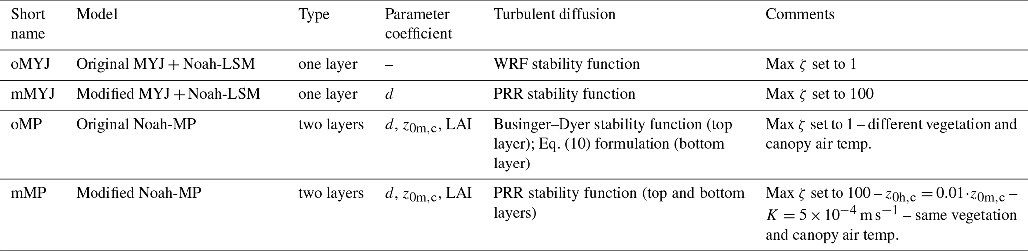
The guiding principle for the modifications to both original models was to improve the modelled dependency of the temperature inversion on the wind speed, in particular the transition between the two regimes. This included removing the imposed maximum on ζ so that a truly stable regime is allowed to develop. The stability function was also modified to a more long-tail formulation (Sect. 3.2): this makes the transition more gradual and avoids the non-monotonicity associated with Eq. (9) at ζ>1. Furthermore, a displacement height is added in the mMYJ model.

Modifications implemented in mMP included forcing the vegetation and canopy air temperature to be equal so that the energy balance for the vegetated part is as described in Sect. 2.1. The canopy-to-ground turbulent diffusion coefficient was also calculated as in the MYJ surface layer instead of using Eq. (10). Lastly, a constant coefficient $K=\mathrm{5}\times {\mathrm{10}}^{-\mathrm{4}}$ m s⁻¹ was added to C_D,aU_a. This effectively imposes a lower limit on the turbulent diffusion coefficient in a gradual way, without having to force a minimum which would create a discontinuity. At wind speeds greater than 3 m s⁻¹, this constant coefficient is negligible compared to the calculated value of C_D,aU_a. It should be noted that in effect, the original Noah-MP also imposes such a limit through indirect methods (for example, by imposing a minimum value of 1 m s⁻¹ for U_a or a maximum value of 1 for ζ). The reasons for imposing a lower limit on the turbulence are explored further in Sect. 5.1.

4.3 Model evaluation

In order to evaluate the models “offline”, the oMYJ and oMP models were extracted from the WRF framework and recoded in Python in a minimal form; i.e. only the parts relating to the surface temperature calculation were kept. In particular, all latent heat flux calculations were ignored; the snow conductivity was assumed to be constant, equal to 0.3 W m⁻¹ K⁻¹, and snow depth and ground temperature were used as input variables rather than being calculated. mMYJ and mMP were similarly coded in Python.

Input parameters to all four models are set to correspond to the characteristics of the PRR site as determined in Sect. 3.2: i.e. d=1.4 m, $z_{\mathrm{0}\mathrm{m},\mathrm{c}}=\mathrm{0.4}$ m and $z_{\mathrm{0}\mathrm{m},\mathrm{s}}=\mathrm{0.002}$ m. For oMP and mMP, f_veg was determined from the LAI using Eq. (12). For the two modified versions, the stability function used is the one determined from the Poker Flat Research Range measurements (Sect. 3.2).

Here, the top of the surface layer was considered to be the top of the measurement tower; i.e. z_a=16 m. The five input variables to the Python models are the measured air temperature at 16 m, wind speed at 16 m, downwards long-wave flux above the canopy, snow depth and ground temperature. The output is the surface temperature (and canopy temperature for the two-layer models). Running the models over the entirety of the curated PRR dataset yielded 5412 modelled values of surface temperature, which were then compared to the corresponding 5412 measured values of T_s. The results are analysed in Sect. 5.2.

5 Results

5.1 Modelled impact of the wind speed on the development of temperature inversions

The outputs of the one-layer models (oMYJ and mMYJ) are shown in blue in Fig. 7c. Both tend to have similar values to the observations for low wind speeds, although oMYJ does not reach a constant regime because ζ is limited to values of 1. Because this limit is removed in mMYJ, it better reproduces two regimes separated by a transition; this transition is however more gradual because the PRR stability function was used. Both models, however, predict too small values of ΔT_as at high wind speeds compared to the observations.

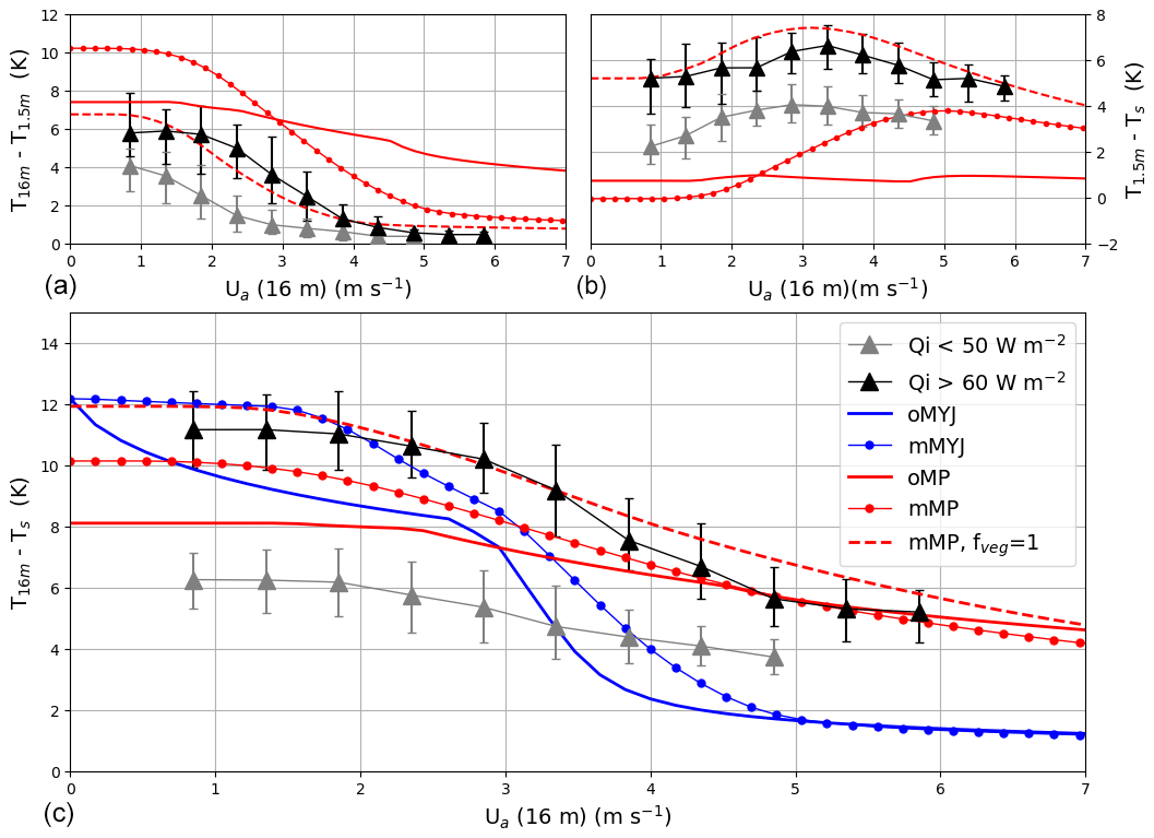
Figure 7 (a) Average temperature difference between z_a=16 and 1.5 m (ΔT_ac) as a function of wind speed at 16 m. The black and grey lines indicate averaged measurements for Q_i>60 W m⁻² and Q_i<50 W m⁻², respectively. (b), (c) The same as (a) but for ΔT_cs and ΔT_as, respectively. The continuous and dotted blue lines correspond to the output of the oMYJ and mMYJ models, respectively, for input values Q_i=65 W m⁻², T_a=263.15 K, T_g=271.15 K and Λ_s=1 W m⁻² K⁻¹ (as already used in the asymptotic model in Fig. 2). The continuous and dotted red lines correspond to the output of the oMP and mMP models, respectively, with the same input values of Q_i, T_a, T_g and Λ_s. The dashed red line corresponds to the same simulation as the dotted red line, except that f_veg=1.

The two-layer models, on the other hand, both show a much more gradual decrease in ΔT_as with U_a. Indeed, the decrease is so gradual in the output of oMP that it is not possible to discern two distinct regimes – even though the stability function used is Businger–Dyer, which is very short tailed (see Fig. 3a, black lines compared to the grey line which corresponds to the PRR stability function). One reason for this is that many limits are placed to maintain turbulence: u^* cannot become larger than 0.07 m s⁻¹; ζ must remain smaller than 1; and when the wind speed is used for calculating the turbulent diffusion coefficient, it takes a minimum value of 1 m s⁻¹ (this is only the case within the surface layer modules so that WRF still outputs wind speed values less than 1 m s⁻¹). Although it is true that some turbulence is always maintained, as shown by the measurements at the PRR site (Fig. 6), the result is that the Noah-MP model outputs too low ΔT_as values at very low wind speeds. oMP also does not reproduce the individual behaviour of ΔT_cs and ΔT_ac: its calculated ΔT_ac does not have an S shape as a function of wind speed, and ΔT_cs exhibits no maximum.

The behaviour of mMP is more satisfactory. ΔT_ac shows a clear transition between a low-wind-speed, high-gradient state and high-wind-speed state where the gradient is close to 0. ΔT_cs has a maximum between 3 and 5 m s⁻¹ (depending on the value of f_veg). ΔT_as, finally, is close to the observed value in both the high- and the low-wind-speed limits. Two things must be noted here: first, that values of ΔT_cs remain positive at low wind speeds because, as noted in Sect. 4.2, a constant K equal to $\mathrm{5}\times {\mathrm{10}}^{-\mathrm{4}}$ m s⁻¹ has been added to C_D,aU_a. Similar to the limits imposed in oMP, this serves to maintain a certain level of turbulence and avoid the collapse of the turbulent sensible heat flux. Without this, ΔT_cs would decrease much more strongly, as described in Sect. 2.1. Adding a constant, as opposed to imposing a maximum value, is a more gradual method which does not distort the shape of the transition. The constant value is chosen to best represent the observations and should be discussed in regard to other datasets.

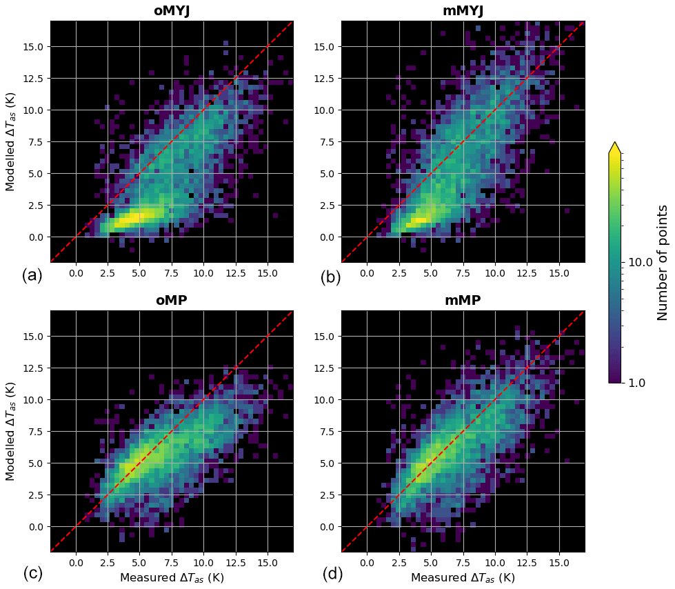
Figure 8 2D histograms of the modelled vs. measured $\mathrm{\Delta }{T}_{\mathrm{as}}=T_{\mathrm{16}\mathrm{m}}-T_{\mathrm{s}}$ for the four models. (a, b) One-layer models (a – oMYJ; b – mMYJ). (c, d) Two-layer models (c – oMP; d – mMP). The colour represents the number of points, in a lognormal scale, and the dashed red line corresponds to the 1:1 line.

Secondly, two versions of mMP are shown in Fig. 7. The first corresponds to f_veg=0.3 and ϵ_v=0.5, which are the values which would be calculated by WRF from a LAI of 0.73 according to Eq. (12). The second corresponds to f_veg=1 and ϵ_v=0.15. The results are substantially different, especially concerning the canopy temperature (and therefore ΔT_cs and ΔT_ac). Indeed, as outlined in Sect. 2.1, the canopy tends to become colder than the surface for higher values of ϵ_v, and this is the case for the simulation with f_veg=0.3. Furthermore, the transition wind speed (for ΔT_ac) and wind speed at maximum ΔT_ac are shifted to lower values for the simulation with f_veg=1. These two sets of values both correspond to ϵ_c=0.15 and therefore to the same radiative flux balance. However, the difference in outcome suggests that due to the turbulent fluxes, separating a bare fraction from a vegetated fraction is not equivalent to considering only one layer but with lower emissivity. The simulation with f_veg=1 seems to perform better. One possible explanation is linked to the size of the eddies transporting heat. If they are of similar size to the typical distance between the trees, the turbulent transport of heat would not necessarily behave differently over a bare fraction than over a vegetated fraction. Instead, all turbulent transport would occur in an averaged manner. Indeed, the turbulent characteristics calculated in Sect. 3.2 are likely representative of this average, depending on the instrument footprint. At the PRR site, average tree distance is approximately 2.2 m, assuming that the trees are homogeneously distributed (which seems reasonable from site photos, Fig. 4). It is, however, not clear whether this is a robust feature of the two-layer models. Indeed, oMP does not appear to perform better when f_veg is set to 1 and ϵ_c to 0.15: its calculated values of ΔT_as decrease more rapidly with wind speed and therefore remain smaller than the measured temperature difference over the whole wind speed range (not shown). In the following, the values of f_veg=0.3 and ϵ_v=0.5 are used for both two-layer models.

5.2 Evaluation of WRF SEB-SL model compared to the PRR site measurements

The models are then run over all the PRR measurement points. Compared to the above analysis, this makes it possible to evaluate their behaviour for a wide variety of input values. Overall, all models capture some of the variability in ΔT_as, probably due to the influence of the downwards radiative fluxes. It is clear however that the one-layer models always underestimate ΔT_as when the measured ΔT_as is the lowest, which corresponds to conditions of high wind speeds (Fig. 8). oMYJ also underestimates ΔT_as when the measured ΔT_as is very high, but this effect has been corrected in mMYJ by allowing for a stronger decrease in turbulence. The root mean square error (RMSE) of mMYJ is therefore approximately 2.8 K as opposed to 3.4 K for the original MYJ scheme.

The two-layer models both perform better than the one-layer models, supporting the idea that they are more adapted for use in a forest environment. The original Noah-MP model cannot reproduce strong values of ΔT_as because of excessive forced turbulence; mMP fares better in that regard. Its RMSE is slightly better (2.2 instead of 2.3 K). Note that running mMP with f_veg=1 and ϵ_v=0.15 leads to an RMSE of 2.1 K. To gain insight into the reliability of the model, all available observations are selected and binned according to their wind speed U_a values in intervals of width of 0.5 m s⁻¹. This eliminates assumptions regarding input parameters such as the net radiation at the surface. Results are shown in Fig. 9.

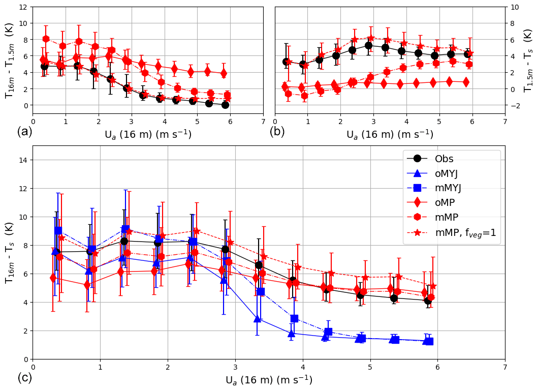
Figure 9 (a) Median temperature difference between z_a=16 m and 1.5 m (ΔT_ac) as a function of wind speed at 16 m. The black line indicates measurements binned according to their wind speed U_a values in intervals of width of 0.5 m s⁻¹. (b), (c) The same as (a) but for ΔT_cs and ΔT_as, respectively. The continuous and dotted blue lines correspond to the output of the oMYJ and mMYJ models, respectively. The continuous and dotted red lines correspond to the output of the oMP and mMP models, respectively. The dashed red line corresponds to the same simulation as the dotted red line, except that f_veg=1. The error bars on the measured and modelled values represent the interquartile range (25th and 75th percentiles).

It clearly shows that MYJ, whether in its original (oMYJ) or its modified (mMYJ) versions, reproduces a too sharp transition due to the fact that it only considers a single layer and strongly differs from the observations when U_a values become larger than 2.5 m s⁻¹. mMYJ is in better agreement with the observations when the wind speed is weaker because the modelled ΔT_as values are obtained in a constant regime and enhanced by 2 K. This is the consequence of removing the limitation of ζ values to 1.

Regarding the two-layer models, oMP slightly underestimates the strength of the inversion for small values of the wind speed U_a, even though the results are not too far from the error bars: the interquartile intervals barely overlap with those of the observed values. On the other hand, it appears obvious that it is actually due to compensation errors in the two layers taken individually: ΔT_ac is overestimated, while ΔT_cs is underpredicted.

The two versions of mMP by far provide the best results compared to the observations, especially when f_veg=1 (Fig. 9). It captures the dependency of the two individual layers (atmosphere–canopy and canopy–surface) on the wind speed well. A key result is that the transition between the two modes is much more gradual in two-layer models. Over a forest area or in multi-layer models, the S shape, reported in one-layer models, becomes blurred: this smoother transition between the two modes can be ascribed to the presence of trees, which attenuates the S shape. This is the reason why two-layer models perform better.

6 Conclusions and perspectives

A simple two-layer analytical model of the stable surface layer was developed and contrasted with the existing one-layer models of van de Wiel et al. (2017). The two-layer model predicted a more gradual dependency of ΔT_as on the wind speed than the one-layer models with equivalent roughness lengths and stability function. The top layer exhibited the S-shape dependence of the temperature gradient on the wind speed, which is typical of one-layer models. The bottom layer, on the other hand, had a maximum temperature gradient at the transition wind speed. However, results depended strongly on the value of the first layer emissivity. Insights gained from the theoretical models were applied to study two surface layer/land surface model modules in WRF: Noah-MP and the Noah-MYJ combination. It was found that these models tend to set very restrictive boundaries on the turbulent diffusion coefficients and stability parameters so that strong temperature gradients cannot be reached.

A combined approach was then used to study the performance of different surface layer models in more detail. First, an extensive set of measurements from the Poker Flat Research Range was analysed. It was found that under clear-sky, snow-covered nighttime conditions, the temperature gradient depended strongly on both the downwards long-wave flux and the wind speed. When the wind speed at 16 m was smaller than 2 m s⁻¹, the temperature profile showed a very strong inversion down to the surface, and the Richardson number was larger than 0.25, the traditional “cutoff” value for turbulence. Nevertheless, some turbulent sensible heat flux remained. On the other hand, when the wind speed was larger than 4 m s⁻¹, the temperature profile was roughly constant down to 1.5 m, below which a strong temperature gradient remained. The Richardson number was then below 0.25, corresponding to the traditional weakly stable regime. Furthermore, the dependence of the individual-layer temperature inversion on wind speed was qualitatively similar to the theoretical two-layer model.

Four different SEB-SL models were then coded into Python: the Noah-MYJ combination, Noah-MP and modified versions of the two. These were first compared to the observations qualitatively and then by inputting measured values of temperature and wind speed at different altitudes into the surface layer and comparing the outputted value of ΔT_as to the measurements. It was found that the two-layer models both gave better results than the one-layer models, which tended to predict too low temperature gradients at high wind speeds. Over a forest area, the presence of trees indeed tends to attenuate the transition between the two modes. On the other hand, the original Noah-MP predicted too low temperature gradients at low wind speeds. All in all, the modified Noah-MP gave the best results, especially for the individual-layer temperature gradients.

Open questions remain concerning the impact of local parameters on the simulations. Although the PRR site is classified as evergreen needleleaf forest by the MODIS land use categories, its characteristics are actually rather similar to a wooded or mixed tundra: its trees are indeed very short and spaced out, and its emissivity and roughness length are quite low for a forest site. These parameters were shown to impact the behaviour of the lowest-layer temperature gradient. Indeed, at high emissivities, the canopy layer is theoretically predicted to become colder than the surface. Furthermore, the value of the turbulent diffusion parameter for the surface-to-canopy air heat exchanges is taken from Monin–Obukhov similarity theory, which assumes a log-wind profile. Other parametrisations, such as the logarithmic and exponential profiles of Mahat et al. (2013), which are implemented in Noah-MP, could conceivably yield better results in a denser forest. It would therefore be necessary to test the behaviour of the model compared to a denser forest site with higher trees.

This study focuses on the clear-sky surface layer in an Arctic winter context. Clear-sky periods have been identified as those when the net long-wave radiation was less than −30 W m⁻² (Graham et al., 2017; Maillard et al., 2021). Wintertime conditions have been selected in periods between November and March when the downwelling short-wave radiation was lower than 30 W m⁻², the latent heat flux less than 5 W m⁻² and the snow depth greater than 10 cm. Outside these conditions, the original conceptual models have not been modified. The implementation of conceptual model improvements in WRF should be followed by a testing phase to find out how the mesoscale model performs outside these restrictive conditions.

The major perspective arising from the present paper is the implementation of the modified SEB-SL models into the main WRF framework. Once this is done, the impact of the modifications on model output can be tested over real cases. Because wind speed can vary locally due to topography in the continental Arctic, the modifications suggested here are therefore expected to impact the spatial distribution of near-surface SBIs during winter anticyclonic episodes, with resulting consequences for the modelling of pollutant dispersion and pollution episodes. Another major question concerns the impact of clouds on the surface layer stability and SBI and how transitions between cloudy- and clear-surface layers are represented by WRF.

Appendix A: Conceptual two-layer model development

The surface energy balance corresponding to the system in Fig. 1 is

$$\begin{array}{}\text{(A1)}& {\text{LW}}_{\mathrm{d},\mathrm{bc}}-{\text{LW}}_{\mathrm{u},\mathrm{bc}}+G+H_{\mathrm{c}}=\mathrm{0},\end{array}$$

where LW_d,bc and LW_u,bc are the downwards and upwards fluxes below the canopy level, G is the ground heat flux, and H_c is the turbulent sensible heat exchange between the canopy and the surface. Each flux can then be parametrised as follows:

$$\begin{array}{ll}{\displaystyle }{\text{LW}}_{\mathrm{d},\mathrm{bc}}& {\displaystyle }=(\mathrm{1}-{\mathit{ϵ}}_{\mathrm{c}}){\text{LW}}_{\mathrm{d}}+{\mathit{ϵ}}_{\mathrm{c}}\mathit{\sigma }{T}_{\mathrm{c}}^{\mathrm{4}}\\ \text{(A2)}& {\displaystyle }{\text{LW}}_{\mathrm{u},\mathrm{bc}}& {\displaystyle }=\mathit{\sigma }{T}_{\mathrm{s}}^{\mathrm{4}},\end{array}$$

where ϵ_c is the canopy emissivity, T_c the canopy temperature, T_s the surface temperature and LW_d the downwards long-wave flux above the canopy level. If T_a is the air temperature above the canopy, T_c can be written as $T_{\mathrm{c}}=T_{\mathrm{a}}+\mathit{\delta }$, where $\mathit{\delta }=T_{\mathrm{c}}-T_{\mathrm{a}}$. Hence $T_{\mathrm{c}}^{\mathrm{4}}=T_{\mathrm{a}}^{\mathrm{4}}{\left(\mathrm{1}+{\displaystyle \frac{\mathit{\delta }}{T_{\mathrm{a}}}}\right)}^{\mathrm{4}}$, assuming that $\left|\mathit{\delta }\right|\ll T_{\mathrm{a}}$. A first-order Taylor expansion leads to $T_{\mathrm{c}}^{\mathrm{4}}\approx T_{\mathrm{a}}^{\mathrm{4}}\left(\mathrm{1}+\mathrm{4}{\displaystyle \frac{\mathit{\delta }}{T_{\mathrm{a}}}}\right)\approx T_{\mathrm{a}}^{\mathrm{4}}+\mathrm{4}{T}_{\mathrm{a}}^{\mathrm{3}}(T_{\mathrm{c}}-T_{\mathrm{a}})$.
Similarly, $T_{\mathrm{s}}^{\mathrm{4}}\approx T_{\mathrm{a}}^{\mathrm{4}}+\mathrm{4}{T}_{\mathrm{a}}^{\mathrm{3}}(T_{\mathrm{s}}-T_{\mathrm{a}})$.

$$\begin{array}{}\text{(A3)}& H_{\mathrm{c}}=-\mathit{\rho }{C}_p{C}_{\mathrm{D},\mathrm{c}}{U}_{\mathrm{c}}(T_{\mathrm{s}}-T_{\mathrm{c}}),\end{array}$$

where ρ is the air density, C_p the heat capacity of air, U_c the canopy wind speed and C_D,c the turbulent diffusion coefficient for the surface-to-canopy sensible heat exchange.

$$\begin{array}{}\text{(A4)}& G=-{\displaystyle \frac{{\mathit{\lambda }}_{\mathrm{s}}}{d_{\mathrm{s}}}}(T_{\mathrm{s}}-T_{\mathrm{g}})={\mathrm{\Lambda }}_{\mathrm{s}}(T_{\mathrm{g}}-T_{\mathrm{a}}+\mathrm{\Delta }{T}_{\mathrm{ac}}+\mathrm{\Delta }{T}_{\mathrm{cs}}),\end{array}$$

where λ_s is the snow conductivity, d_s the snow depth and T_g the ground temperature. The surface energy balance equation can then be reorganised to Eq. (1):

$$\begin{array}{}\text{(A5)}& \begin{array}{rl}-(\mathrm{1}-{\mathit{ϵ}}_{\mathrm{c}})Q_{\mathrm{i}}-{\mathrm{\Lambda }}_{\mathrm{s}}(T_{\mathrm{a}}-T_{\mathrm{g}})& +\mathrm{\Delta }{T}_{\mathrm{cs}}\left[\mathit{\rho }{C}_p{C}_{\mathrm{D},\mathrm{c}}{U}_{\mathrm{c}}+\mathrm{4}\mathit{\sigma }{T}_{\mathrm{a}}^{\mathrm{3}}+{\mathrm{\Lambda }}_{\mathrm{s}}\right]\\ & +\mathrm{\Delta }{T}_{\mathrm{ac}}\left[(\mathrm{1}-{\mathit{ϵ}}_{\mathrm{c}})\mathrm{4}\mathit{\sigma }{T}_{\mathrm{a}}^{\mathrm{3}}+{\mathrm{\Lambda }}_{\mathrm{s}}\right]\\ & =\mathrm{0}.\end{array}\end{array}$$

Similarly, the energy balance applied to the canopy layer yields

$$\begin{array}{}\text{(A6)}& {\text{LW}}_{\mathrm{d}}-{\text{LW}}_{\mathrm{u}}-({\text{LW}}_{\mathrm{d},\mathrm{bc}}-{\text{LW}}_{\mathrm{u},\mathrm{bc}})+H_{\mathrm{a}}-H_{\mathrm{c}}=\mathrm{0},\end{array}$$

where LW_u is the upwards long-wave flux measured above the canopy level.

$$\begin{array}{}\text{(A7)}& H_{\mathrm{a}}=-\mathit{\rho }{C}_p{C}_{\mathrm{D},\mathrm{a}}{U}_{\mathrm{a}}(T_{\mathrm{c}}-T_{\mathrm{a}}),\end{array}$$

where U_a is the air wind speed and C_D,a the turbulent diffusion coefficient for the canopy-to-air sensible heat exchange. The downwards fluxes can be written as

$$\begin{array}{}\text{(A8)}& \begin{array}{rl}{\text{LW}}_{\mathrm{d}}-{\text{LW}}_{\mathrm{d},\mathrm{bc}}& ={\mathit{ϵ}}_{\mathrm{c}}{\text{LW}}_{\mathrm{d}}-{\mathit{ϵ}}_{\mathrm{c}}\mathit{\sigma }{T}_{\mathrm{c}}^{\mathrm{4}}\\ & \approx {\mathit{ϵ}}_{\mathrm{c}}({\text{LW}}_{\mathrm{d}}+\mathrm{4}\mathit{\sigma }{T}_{\mathrm{a}}^{\mathrm{3}}\mathrm{\Delta }{T}_{\mathrm{ac}}-\mathit{\sigma }{T}_{\mathrm{a}}^{\mathrm{4}})\\ & \approx -{\mathit{ϵ}}_{\mathrm{c}}Qi+\mathrm{4}{\mathit{ϵ}}_{\mathrm{c}}\mathit{\sigma }{T}_{\mathrm{a}}^{\mathrm{3}}\mathrm{\Delta }{T}_{\mathrm{ac}}.\end{array}\end{array}$$

Similarly, the algebraic sum of the upwards fluxes is

$$\begin{array}{}\text{(A9)}& {\text{LW}}_{\mathrm{u},\mathrm{bc}}-{\text{LW}}_{\mathrm{u}}={\mathit{ϵ}}_{\mathrm{c}}\mathit{\sigma }(T_{\mathrm{s}}^{\mathrm{4}}-T_{\mathrm{c}}^{\mathrm{4}})\approx -\mathrm{4}{\mathit{ϵ}}_{\mathrm{c}}\mathit{\sigma }{T}_{\mathrm{a}}^{\mathrm{3}}\mathrm{\Delta }{T}_{\mathrm{cs}}.\end{array}$$

This transforms to

$$\begin{array}{}\text{(A10)}& \begin{array}{rl}-{\mathit{ϵ}}_{\mathrm{c}}{Q}_{\mathrm{i}}& -\mathrm{\Delta }{T}_{\mathrm{cs}}\left[\mathit{\rho }{C}_p{C}_{\mathrm{D},\mathrm{c}}{U}_{\mathrm{c}}+\mathrm{4}{\mathit{ϵ}}_{\mathrm{c}}\mathit{\sigma }{T}_{\mathrm{a}}^{\mathrm{3}}\right]\\ & +\mathrm{\Delta }{T}_{\mathrm{ac}}\left[\mathit{\rho }{C}_p{C}_{\mathrm{D},\mathrm{a}}{U}_{\mathrm{a}}+\mathrm{4}{\mathit{ϵ}}_{\mathrm{c}}\mathit{\sigma }{T}_{\mathrm{a}}^{\mathrm{3}}\right]=\mathrm{0}.\end{array}\end{array}$$

Summing Eqs. (1) and (A10) then yields Eq. (2):

$$\begin{array}{}\text{(A11)}& \begin{array}{rl}-Q_{\mathrm{i}}-{\mathrm{\Lambda }}_{\mathrm{s}}(T_{\mathrm{a}}-T_{\mathrm{g}})& +\mathrm{\Delta }{T}_{\mathrm{cs}}\left[(\mathrm{1}-{\mathit{ϵ}}_{\mathrm{c}})\mathrm{4}\mathit{\sigma }{T}_{\mathrm{a}}^{\mathrm{3}}+{\mathrm{\Lambda }}_{\mathrm{s}}\right]\\ & +\mathrm{\Delta }{T}_{\mathrm{ac}}\left[\mathrm{4}\mathit{\sigma }{T}_{\mathrm{a}}^{\mathrm{3}}+{\mathrm{\Lambda }}_{\mathrm{s}}+\mathit{\rho }{C}_p{C}_{\mathrm{D},\mathrm{a}}{U}_{\mathrm{a}}\right]\\ & =\mathrm{0}.\end{array}\end{array}$$