DCMIP2016: the tropical cyclone test case

This paper describes and analyzes the Reed–Jablonowski (RJ) tropical cyclone (TC) test case used in the 2016 Dynamical Core Model Intercomparison Project (DCMIP2016). This intermediate-complexity test case analyzes the evolution of a weak vortex into a TC in an idealized tropical environment. Reference solutions from nine general circulation models (GCMs) with identical simplified physics parameterization packages that participated in DCMIP2016 are analyzed in this study at 50 km horizontal grid spacing, with five of these models also providing solutions at 25 km grid spacing. Evolution of minimum surface pressure (MSP) and maximum 1 km azimuthally averaged wind speed (MWS), the wind–pressure relationship, radial profiles of wind speed and surface pressure, and wind composites are presented for all participating GCMs at both horizontal grid spacings. While all TCs undergo a similar evolution process, some reach significantly higher intensities than others, ultimately impacting their horizontal and vertical structures. TCs simulated at 25 km grid spacings retain these differences but reach higher intensities and are more compact than their 50 km counterparts. These results indicate that dynamical core choice is an essential factor in GCM development, and future work should be conducted to explore how specific differences within the dynamical core affect TC behavior in GCMs.

1 Introduction

Tropical cyclones (TCs) are among the most dangerous meteorological phenomena in the world, causing billions of dollars in damage annually and significantly impacting both coastal and offshore regions (Emanuel, 2003). TC behavior is expected to change with global warming, with the most confident projection being increased storm surge levels and flooding due to higher sea levels (Knutson et al., 2020). There is evidence that TC global average intensity, precipitation rates, and the proportion of storms reaching high intensities (categories 4 and 5 on the Saffir–Simpson scale) may increase in the future (Knutson et al., 2020). Increases in the proportion of category 4 and 5 TCs and the global average intensity of these high-intensity TCs in past observational data signal that anthropogenic signals may have already been observed (Knutson et al., 2019). Simulating TCs accurately in general circulation models (GCMs) allows for current and future risks to be better understood and leads to improved mitigation of these risks.

Simulating TCs in GCMs is complicated and requires both extensive computational power and sophisticated simulations. Although the grid spacing of a GCM of the typical Coupled Model Intercomparison Project (CMIP) class is around 100 km, TCs are not well resolved when the grid spacing is coarser than 50 km due to their small size and the complex physical processes that cause their formation and propagation (Reed and Jablonowski, 2011a). TC intensity, size, and genesis generally become more accurate with increasing horizontal resolution (Reed and Jablonowski, 2011a, b), a trend that has also been shown in decadal climate-scale simulations (Wehner et al., 2014; Stansfield et al., 2020; Roberts et al., 2020). This trend has also been shown for the TC test case developed in Reed and Jablonowski (2011a, 2012), hereafter referred to as the Reed–Jablonowski (RJ) TC test case, since it increases in intensity and becomes more compact with increasing horizontal resolution (Reed and Jablonowski, 2011a). The RJ TC test case is a moist deterministic test case designed to be used in simple-physics experiments with intermediate complexity (between dry-dynamical-core and full-physics aquaplanet simulations). This test case provides a less complex regime to study how the dynamical core and moist physical parameterizations interact without having to conduct a computationally expensive simulation (Reed and Jablonowski, 2012).

There are several studies that demonstrate the usefulness of studying the RJ TC test case formulation. Reed and Jablonowski (2011c) found that the RJ TC test case increases in strength and size, while having an earlier onset of intensification in the Community Atmosphere Model (CAM) version 4 (CAM4), developed by the National Center for Atmospheric Research (NCAR), compared to its predecessor CAM3 due to the presence of a dilute-plume convective available potential energy (CAPE) calculation in CAM4. Additionally, Reed and Jablonowski (2011b) illustrate how uncertainties in the RJ TC test case simulations can be structural, parameter-based, or initial-data-based, with structural uncertainties being the most prominent when CAM4 and CAM5 are compared. This study did not take into account structural differences in the dynamical cores of the models, the components that integrate the Navier–Stokes equations, likely underestimating structural uncertainty (Reed and Jablonowski, 2011b). Reed and Jablonowski (2012) investigate how the dynamical core choice impacts the RJ TC test case structure and intensity in simple-physics simulations and complex CAM5 full-physics aquaplanet simulations with grid spacings of approximately 50 km or less. This work indicates that simple-physics experiments can provide meaningful insight into how dynamical core characteristics impact simulated TC behavior. In CAM5 comprehensive climate-scale simulations, the spectral element dynamical core produces more TCs that tend to have stronger intensities than those produced in a simulation using the finite-volume dynamical core (Reed et al., 2015). This result is consistent with the RJ TC test case analysis in Reed and Jablonowski (2012), demonstrating further confidence in the use of idealized test cases and intermediate-complexity simulations to better understand the impact of GCM design on simulated TC characteristics.

Other GCM characteristics have been shown to have a significant impact on the resulting behavior of the RJ TC test case. The grid spacing of the model is critical to the simulation of certain characteristics in the test case, with higher-resolution models creating increasingly intense and compact TCs that can even demonstrate non-physical intensity due to the physics parameterization behavior at small time steps (Reed et al., 2012). He et al. (2018) use Sobol' variance-based sensitivity analysis to analyze input–output relationships that are multivariate in nature and demonstrate that resolution significantly impacts sensitivities to control factors, with coarse-resolution simulations unable to produce an accurate TC. This study also found nonlinear relationships between factors that control precipitation rate, cloud content, and radiative forcing in the idealized RJ TC test case. He and Posselt (2015) demonstrate how the parameterized physical processes in cloud formation, convective development, and moist turbulence impact the simulation of TC intensity, precipitation rate, and other characteristics during the evolution of the RJ TC test case in CAM5, with nonlinear relationships occurring between certain parameters and output variables. In CAM5, the precipitation and intensity of the simulated TCs are sensitive to the physics–dynamics time step, with the magnitude of the sensitivities dependent on the dynamical core and horizontal resolution used (Li et al., 2020).

The 2016 Dynamical Core Model Intercomparison Project (DCMIP2016) (Ullrich et al., 2017) aims to increase knowledge about how the dynamical core of a GCM impacts the behavior of various meteorological test cases. The test cases used in DCMIP2016 (Ullrich et al., 2016) include simplified moist physics and build upon the previous sets of test cases developed for DCMIP2012 (Ullrich et al., 2012) and DCMIP2008 (Jablonowski et al., 2008). These test cases include a moist baroclinic wave, a splitting supercell (Zarzycki et al., 2019), and the RJ TC test case. While past studies have explored dynamical core impact on TC behavior, they largely focus on a single model. A model intercomparison facilitates detailed comparison and documentation of TC behavior among different GCMs, which have differences in their dynamical core design such as horizontal and vertical discretization, time stepping, native grid, and grid staggering (Ullrich et al., 2017). Reference solutions provided by model intercomparison contribute to the improvement of GCMs and lead to more accurate simulations of TCs. This study provides an intercomparison of RJ TC test case behavior among the DCMIP2016 models. The goal of this analysis is to provide a library of solutions that serve as a benchmark for modeling groups to compare with and does not aim to link differences in results to specific numerical differences in the models. There is no ground truth to this test case, and the RJ TC test case and other DCMIP test cases are in wide use among modeling groups. Standardized test suites are essential for model development, and specific use cases for these tests include verifying the performance of dynamical cores in their operational states and providing assessments of convergence at finer grid spacing and uncertainty between solutions of several models. Further, several DCMIP test cases are implemented as part of the Community Earth System Model (CESM) Simpler Models framework, which allows researchers to gain insight into atmospheric phenomena through simple, often idealized, model frameworks (CES, 2023).

In Sect. 2, we provide a detailed explanation of the initialization of the RJ TC test case along with the analytical and computational procedures used throughout this study. In Sect. 3, we catalog similarities and differences in the RJ TC test case behavior among participating GCMs. Specifically, we analyze the evolution of maximum 1 km (measured from the surface) azimuthally averaged wind speed (MWS) and minimum surface pressure (MSP), radial profiles and vertical composites of wind speed and surface pressure, and the wind–pressure relationship. Differences between the 50 km and the 25 km simulations are then discussed for models that submitted simulations at both grid spacings. Section 4 summarizes important results from the model intercomparison and provides a motivation for future work in this area.

2 Methods

2.1 Description of test case

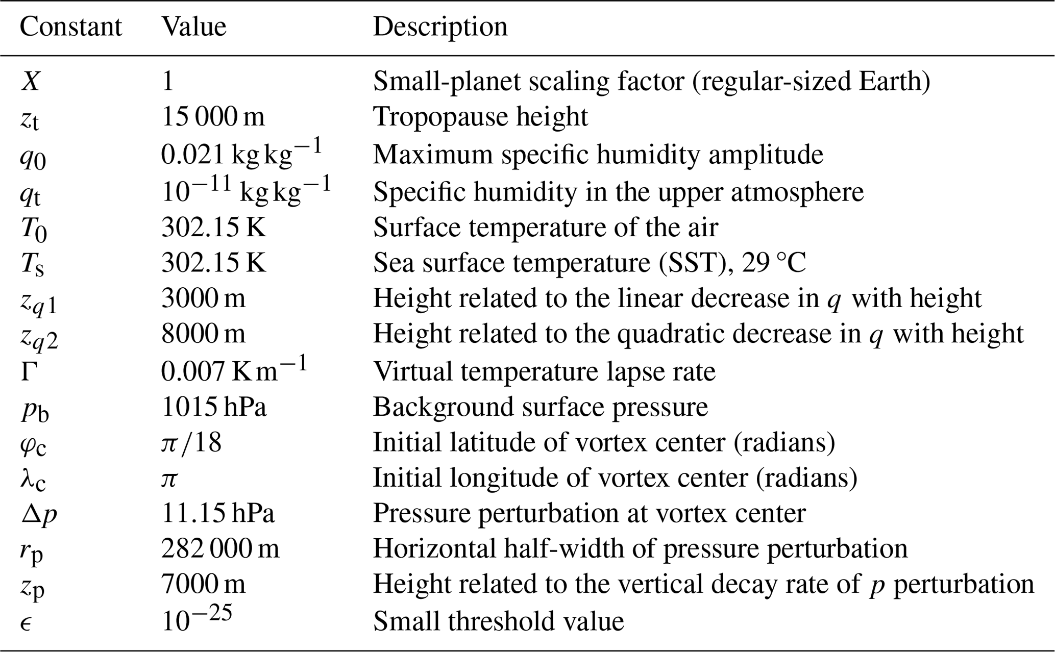
The RJ TC test case is based on the work of Reed and Jablonowski (2011a, 2012). A weak, balanced vortex is initialized in an environment conducive to intensification and evolves into a TC over a 10 d period. GCMs with identical simplified physical parameterization packages simulated this test case in a controlled testing environment to allow for the analysis of dynamical core impact on TC structure and intensity (Ullrich et al., 2016). For reproducibility, lists of DCMIP2016 model initialization symbols, physical constants, and RJ TC test case constants are shown in Tables 1, 2, and 3, respectively. The complete mathematical description of the initialization and axisymmetric vortex of the RJ TC test case is in the subsequent sections.

Table 1 List of DCMIP2016 symbols used in the RJ TC test case initialization (Ullrich et al., 2016).

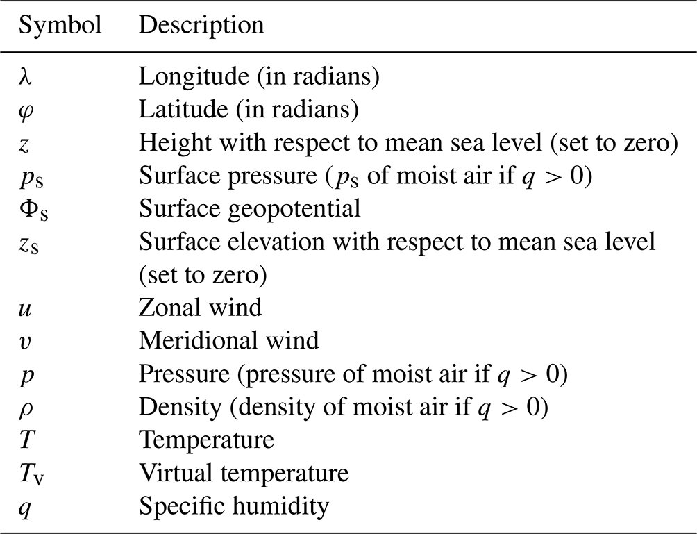
Table 2 A list of physical constants used in DCMIP2016 (Ullrich et al., 2016).

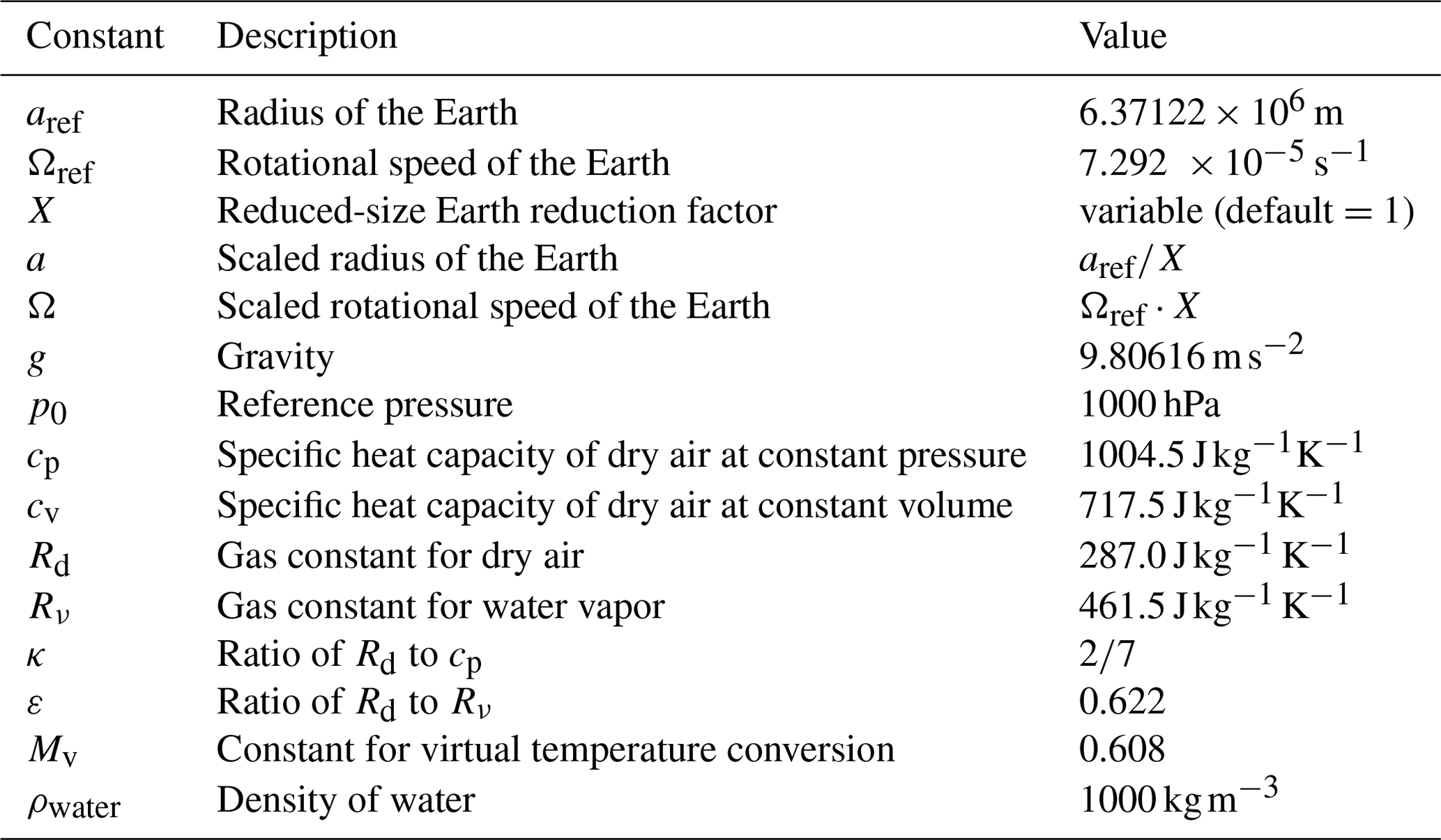
Table 3 List of constants used for the idealized tropical cyclone test (Ullrich et al., 2016).

2.1.1 Environmental background

The RJ TC test case is initialized in the following manner. It contains a background state that consists of three profiles: prescribed specific humidity, virtual temperature, and pressure. The initial profile is in an approximate gradient–wind balance state by definition. The vertical sounding is chosen to approximately resemble an observed tropical sounding (Jordan, 1958). The background specific humidity profile $\stackrel{\mathrm{‾}}{q}\left(z\right)$ as a function of height z is

$$\begin{array}{}\text{(1)}& \begin{array}{rl}\stackrel{\mathrm{‾}}{q}\left(z\right)& =q_{\mathrm{0}}\exp \left(-{\displaystyle \frac{z}{z_{q\mathrm{1}}}}\right)\exp \left[-{\left({\displaystyle \frac{z}{z_{q\mathrm{2}}}}\right)}^{\mathrm{2}}\right]\\ & \text{ for }\mathrm{0}\le z\le z_{\mathrm{t}},\\ \stackrel{\mathrm{‾}}{q}\left(z\right)& =q_{\mathrm{t}}\text{ for }{z}_{\mathrm{t}}\le z.\end{array}\end{array}$$

The specific form of the background virtual temperature sounding ${\stackrel{\mathrm{‾}}{T}}_{\mathrm{v}}\left(z\right)$ is dependent on its location in the atmosphere. In this case, there are two different representations, one for the lower atmosphere and another for the upper atmosphere. They are given by

$$\begin{array}{}\text{(2)}& \begin{array}{ll}{\stackrel{\mathrm{‾}}{T}}_{\mathrm{v}}\left(z\right)=T_{\text{v0}}-\mathrm{\Gamma }z& \text{for }\mathrm{0}\le z\le z_{\mathrm{t}},\\ {\stackrel{\mathrm{‾}}{T}}_{\mathrm{v}}\left(z\right)=T_{\text{vt}}=T_{\text{v0}}-\mathrm{\Gamma }{z}_{\mathrm{t}}& \text{for }{z}_{\mathrm{t}}<z,\end{array}\end{array}$$

with the virtual temperature at the surface calculated as T_v0 = T₀(1+0.608q₀) and the virtual temperature at the tropopause level as $T_{\text{vt}}=T_{\text{v0}}-\mathrm{\Gamma }{z}_{\mathrm{t}}$. The background temperature profile can be obtained from the equation:

$$\begin{array}{}\text{(3)}& T_{\mathrm{v}}=T(\mathrm{1}+M_{\mathrm{v}}q).\end{array}$$

The background vertical pressure profile $\stackrel{\mathrm{‾}}{p}\left(z\right)$ of the moist air can be calculated using the hydrostatic balance and Eq. (2). The profile is given by

$$\begin{array}{}\text{(4)}& \begin{array}{ll}\stackrel{\mathrm{‾}}{p}\left(z\right)=p_{\mathrm{b}}{\left({\displaystyle \frac{T_{\text{v0}}-\mathrm{\Gamma }z}{T_{\text{v0}}}}\right)}^{\frac{g}{R_{\mathrm{d}}\mathrm{\Gamma }}}& \text{for }\mathrm{0}\le z\le z_{\mathrm{t}},\\ \stackrel{\mathrm{‾}}{p}\left(z\right)=p_{\mathrm{t}}\exp \left({\displaystyle \frac{g(z_{\mathrm{t}}-z)}{R_{\mathrm{d}}{T}_{\text{vt}}}}\right)& \text{for }{z}_{\mathrm{t}}<z.\end{array}\end{array}$$

The pressure at the tropopause level z_t is continuous and given by

$$\begin{array}{}\text{(5)}& p_{\mathrm{t}}=p_{\mathrm{b}}{\left({\displaystyle \frac{T_{\text{vt}}}{T_{\text{v0}}}}\right)}^{\frac{g}{R_{\mathrm{d}}\mathrm{\Gamma }}}.\end{array}$$

This value is approximately 130.5 hPa for the set of parameters used in the test case initialization.

2.1.2 Axisymmetric vortex

The pressure p(r,z) for the moist air is composed of the background pressure profile (Eq. 4) and a 2D pressure perturbation $p^{\prime }(r,z)$:

$$\begin{array}{}\text{(6)}& p(r,z)=\stackrel{\mathrm{‾}}{p}\left(z\right)+p^{\prime }(r,z),\end{array}$$

where r symbolizes the radial distance (or radius) from the center of the prescribed vortex. On the sphere, r is defined using the great circle distance (GCD):

$$\begin{array}{}\text{(7)}& r=a\arccos \left(\sin {\mathit{\phi }}_{\mathrm{c}}\sin \mathit{\phi }+\cos {\mathit{\phi }}_{\mathrm{c}}\cos \mathit{\phi }\cos (\mathit{\lambda }-{\mathit{\lambda }}_{\mathrm{c}})\right).\end{array}$$

The pressure perturbation is defined as

$$\begin{array}{llll}{\displaystyle }& {\displaystyle }{p}^{\prime }(r,z)=-\mathrm{\Delta }p\exp \left[-{\left({\displaystyle \frac{r}{r_{\mathrm{p}}}}\right)}^{\mathrm{3}/\mathrm{2}}-{\left({\displaystyle \frac{z}{z_{\mathrm{p}}}}\right)}^{\mathrm{2}}\right]{\left({\displaystyle \frac{T_{\text{v0}}-\mathrm{\Gamma }z}{T_{\text{v0}}}}\right)}^{\frac{g}{R_{\mathrm{d}}\mathrm{\Gamma }}}& {\displaystyle }& {\displaystyle }\\ {\displaystyle }& {\displaystyle }& {\displaystyle }& {\displaystyle }\text{for }\mathrm{0}\le z\le z_{\mathrm{t}},\\ \text{(8)}& {\displaystyle }& {\displaystyle }{p}^{\prime }(r,z)=\mathrm{0}& {\displaystyle }& {\displaystyle }\text{for }{z}_{\mathrm{t}}<z.\end{array}$$

There are several contributions to the pressure perturbation. These include the pressure difference Δp between the background surface pressure p_b and the pressure at the center of the initial vortex, the pressure change in the radial direction, and the pressure decay with height within the vortex. The parameters r_p, the horizontal half-width of the pressure perturbation, and z_p, the height related to the vertical decay rate of the pressure perturbation, describe the shape of the pressure perturbation in these directions. The moist surface pressure p_s(r) is computed by setting z to 0 m in Eq. (6), which gives

$$\begin{array}{}\text{(9)}& p_{\mathrm{s}}\left(r\right)=p_{\mathrm{b}}-\mathrm{\Delta }p\exp \left[-{\left({\displaystyle \frac{r}{r_{\mathrm{p}}}}\right)}^{\mathrm{3}/\mathrm{2}}\right].\end{array}$$

The axisymmetric virtual temperature T_v(r,z) is calculated using the hydrostatic equation and ideal gas law:

$$\begin{array}{}\text{(10)}& T_{\mathrm{v}}(r,z)=-{\displaystyle \frac{gp(r,z)}{R_{\mathrm{d}}}}{\left({\displaystyle \frac{\partial p(r,z)}{\partial z}}\right)}^{-\mathrm{1}}.\end{array}$$

Again, this equation takes the form of a sum of the background state and a perturbation:

$$\begin{array}{}\text{(11)}& T_{\mathrm{v}}(r,z)={\stackrel{\mathrm{‾}}{T}}_{\mathrm{v}}\left(z\right)+T_{\mathrm{v}}^{\prime }(r,z),\end{array}$$

where the virtual temperature perturbation is defined as

$$\begin{array}{llll}{\displaystyle }& {\displaystyle }{T}_{\mathrm{v}}^{\prime }(r,z)=(T_{\text{v0}}-\mathrm{\Gamma }z)\times & {\displaystyle }& {\displaystyle }\\ {\displaystyle }& {\displaystyle }\left\{{\left[\mathrm{1}+{\displaystyle \frac{\mathrm{2}{R}_{\mathrm{d}}(T_{\text{v0}}-\mathrm{\Gamma }z)z}{g{z}_{\mathrm{p}}^{\mathrm{2}}\left[\mathrm{1}-\frac{p_{\mathrm{b}}}{\mathrm{\Delta }p}\exp \left({\left(\frac{r}{r_{\mathrm{p}}}\right)}^{\mathrm{3}/\mathrm{2}}+{\left(\frac{z}{z_{\mathrm{p}}}\right)}^{\mathrm{2}}\right)\right]}}\right]}^{-\mathrm{1}}-\mathrm{1}\right\}& {\displaystyle }& {\displaystyle }\\ {\displaystyle }& {\displaystyle }& {\displaystyle }& {\displaystyle }\text{for }\mathrm{0}\le z\le z_{\mathrm{t}},\\ \text{(12)}& {\displaystyle }& {\displaystyle }{T}_{\mathrm{v}}^{\prime }(r,z)=\mathrm{0}& {\displaystyle }& {\displaystyle }\text{for }{z}_{\mathrm{t}}<z.\end{array}$$

The axisymmetric specific humidity q(r,z) is set to the background profile everywhere:

$$\begin{array}{}\text{(13)}& q(r,z)=\stackrel{\mathrm{‾}}{q}\left(z\right).\end{array}$$

Consequently, the temperature can be written as

$$\begin{array}{}\text{(14)}& T(r,z)=\stackrel{\mathrm{‾}}{T}\left(z\right)+T^{\prime }(r,z),\end{array}$$

with the temperature perturbation defined as

$$\begin{array}{llll}{\displaystyle }& {\displaystyle }{T}^{\prime }(r,z)={\displaystyle \frac{T_{\text{v0}}-\mathrm{\Gamma }z}{\mathrm{1}+\mathrm{0.608}\stackrel{\mathrm{‾}}{q}\left(z\right)}}\times & {\displaystyle }& {\displaystyle }\\ {\displaystyle }& {\displaystyle }\left\{{\left[\mathrm{1}+{\displaystyle \frac{\mathrm{2}{R}_{\mathrm{d}}(T_{\text{v0}}-\mathrm{\Gamma }z)z}{g{z}_{\mathrm{p}}^{\mathrm{2}}\left[\mathrm{1}-\frac{p_{\mathrm{b}}}{\mathrm{\Delta }p}\exp \left({\left(\frac{r}{r_{\mathrm{p}}}\right)}^{\mathrm{3}/\mathrm{2}}+{\left(\frac{z}{z_{\mathrm{p}}}\right)}^{\mathrm{2}}\right)\right]}}\right]}^{-\mathrm{1}}-\mathrm{1}\right\}& {\displaystyle }& {\displaystyle }\\ {\displaystyle }& {\displaystyle }& {\displaystyle }& {\displaystyle }\text{for }\mathrm{0}\le z\le z_{\mathrm{t}},\\ \text{(15)}& {\displaystyle }& {\displaystyle }{T}^{\prime }(r,z)=\mathrm{0}& {\displaystyle }& {\displaystyle }\text{for }{z}_{\mathrm{t}}<z.& {\displaystyle }\end{array}$$

The upper troposphere has a small specific humidity value (10⁻¹¹ kg kg⁻¹ for z>z_t); therefore, the virtual temperature approximately equals the temperature for this portion of the atmosphere. The formulation introduced here is equivalent to the one explained in Reed and Jablonowski (2012).

In some cases, the density of the moist air needs to be initialized as well. The ideal gas law forms the basis of this initialization, and the density of the moist air is initialized in the following manner:

$$\begin{array}{}\text{(16)}& \mathit{\rho }(r,z)={\displaystyle \frac{p(r,z)}{R_{\mathrm{d}}{T}_{\mathrm{v}}(r,z)}},\end{array}$$

which utilizes the moist pressure (Eq. 6) and virtual temperature (Eq. 11). The surface elevation z_s and thereby the surface geopotential Φ_s=gz_s are set to zero.

Finally, gradient–wind balance, a function of pressure (Eq. 6) and the virtual temperature (Eq. 12), allows for the definition of the tangential velocity field v_T(r,z) of the axisymmetric vortex. The tangential velocity is given by

$$\begin{array}{}\text{(17)}& v_{\mathrm{T}}(r,z)=-{\displaystyle \frac{f_{\mathrm{c}}r}{\mathrm{2}}}+\sqrt{{\displaystyle \frac{f_{\mathrm{c}}^{\mathrm{2}}{r}^{\mathrm{2}}}{\mathrm{4}}}+{\displaystyle \frac{R_{\mathrm{d}}{T}_{\mathrm{v}}(r,z)r}{p(r,z)}}{\displaystyle \frac{\partial p(r,z)}{\partial r}}},\end{array}$$

where f_c=2Ωsin (φ_c) is the Coriolis parameter at the constant latitude φ_c. Substituting T_v(r,z) and p(r,z) into Eq. (17) gives

$$\begin{array}{llll}{\displaystyle }& {\displaystyle }{v}_{\mathrm{T}}(r,z)=-{\displaystyle \frac{f_{\mathrm{c}}r}{\mathrm{2}}}+& {\displaystyle }& {\displaystyle }\\ {\displaystyle }& {\displaystyle }\sqrt{{\displaystyle \frac{f_{\mathrm{c}}^{\mathrm{2}}{r}^{\mathrm{2}}}{\mathrm{4}}}-{\displaystyle \frac{\frac{\mathrm{3}}{\mathrm{2}}{\left(\frac{r}{r_{\mathrm{p}}}\right)}^{\mathrm{3}/\mathrm{2}}(T_{\text{v0}}-\mathrm{\Gamma }z)R_{\mathrm{d}}}{\mathrm{1}+\frac{\mathrm{2}{R}_{\mathrm{d}}(T_{\text{v0}}-\mathrm{\Gamma }z)z}{g{z}_{\mathrm{p}}^{\mathrm{2}}}-\frac{p_{\mathrm{b}}}{\mathrm{\Delta }p}\exp \left({\left(\frac{r}{r_{\mathrm{p}}}\right)}^{\mathrm{3}/\mathrm{2}}+{\left(\frac{z}{z_{\mathrm{p}}}\right)}^{\mathrm{2}}\right)}}}& {\displaystyle }& {\displaystyle }\\ {\displaystyle }& {\displaystyle }& {\displaystyle }& {\displaystyle }\text{for }\mathrm{0}\le z\le z_{\mathrm{t}},\\ \text{(18)}& {\displaystyle }& {\displaystyle }{v}_{\mathrm{T}}(r,z)=\mathrm{0}& {\displaystyle }& {\displaystyle }\text{for }{z}_{\mathrm{t}}<z.\end{array}$$

The tangential velocity is then separated into its zonal and meridional wind components, $u(\mathit{\lambda },\mathit{\phi },z)$ and $v(\mathit{\lambda },\mathit{\phi },z)$ (Eq. 18). Similar to Nair and Jablonowski (2008), these are calculated in the following way:

$$\begin{array}{}\text{(19)}& {\displaystyle }{d}_{\mathrm{1}}& {\displaystyle }=\sin {\mathit{\phi }}_{\mathrm{c}}\cos \mathit{\phi }-\cos {\mathit{\phi }}_{\mathrm{c}}\sin \mathit{\phi }\cos (\mathit{\lambda }-{\mathit{\lambda }}_{\mathrm{c}}),\text{(20)}& {\displaystyle }{d}_{\mathrm{2}}& {\displaystyle }=\cos {\mathit{\phi }}_{\mathrm{c}}\sin (\mathit{\lambda }-{\mathit{\lambda }}_{\mathrm{c}}),\text{(21)}& {\displaystyle }d& {\displaystyle }=max(\mathit{ϵ},\sqrt{{d_{\mathrm{1}}}^{\mathrm{2}}+{d_{\mathrm{2}}}^{\mathrm{2}}}),\end{array}$$

and are utilized in the projections

$$\begin{array}{}\text{(22)}& {\displaystyle }u(\mathit{\lambda },\mathit{\phi },z)& {\displaystyle }={\displaystyle \frac{v_{\mathrm{T}}(\mathit{\lambda },\mathit{\phi },z)d_{\mathrm{1}}}{d}},\text{(23)}& {\displaystyle }v(\mathit{\lambda },\mathit{\phi },z)& {\displaystyle }={\displaystyle \frac{v_{\mathrm{T}}(\mathit{\lambda },\mathit{\phi },z)d_{\mathrm{2}}}{d}}.\end{array}$$

Value $\mathit{ϵ}={\mathrm{10}}^{-\mathrm{25}}$ is utilized to avoid divisions by zero. In this case, the vertical velocity is set to zero.

2.2 Simulation design

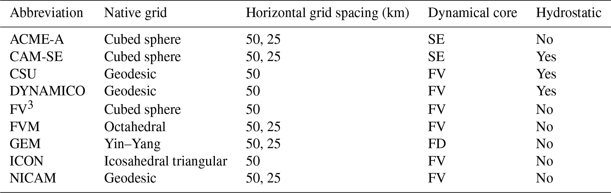
Nine GCMs provided reference solutions for the RJ TC test case as part of DCMIP2016. CSU submitted two versions of their model, CSU-CP and CSU-LZ, which differ in the vertical coordinate. CSU-LZ uses the Lorenz (Lorenz, 1960) staggering of variables in the vertical direction, with potential temperature and advected scalars co-located with horizontal winds at the mid-layer. CSU-CP used the Charney and Phillips (Charney and Phillips, 1953) staggering of variables with potential temperature and advected scalars co-located with the vertical velocity at the layer interfaces. Information about the GCMs studied can be found in Table 4. Models submitted test case solutions prior to 2016 and all results represent their state at that point in time. The GCMs have likely been updated since 2016, but it is still important to provide a set of benchmark solutions for the modeling community. The computational efficiency of each model – that is, the total time to produce a solution at a particular resolution – is not considered here but is nonetheless important since certain models operate at a higher effective resolution with the same computational cost. Certain models are hydrostatic, while others are non-hydrostatic, although this is unlikely to have a significant effect on the simulation (Liu et al., 2022). Information about the GCMs studied including information on dynamical cores and native grids is summarized in Table 5, with further information available in Ullrich et al. (2017).

Table 4 Information about models that submitted RJ TC test case simulations in DCMIP2016 and were analyzed in this study.

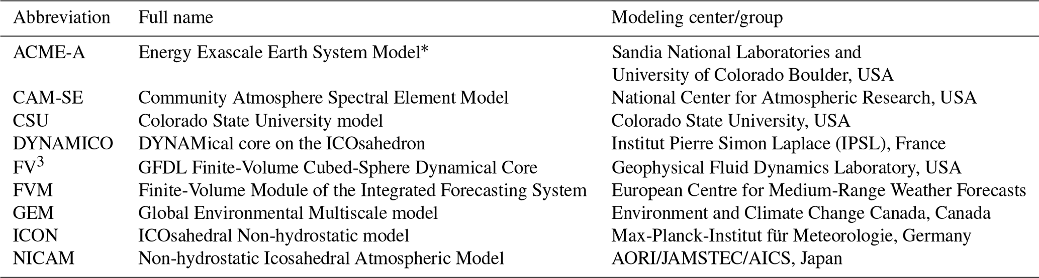
^* The current name of this model is the Energy Exascale Earth System Model and was changed from the Accelerated Climate Model For Energy–Atmosphere in April 2018. Since the ACME-A version was in use at the time of DCMIP2016, ACME-A was used as the abbreviation.

Table 5 Information about the models used in this study. Three dynamical cores are present: spectral element (SE), finite-difference (FD), and finite-volume (FV). More information on dynamical cores and model-specific processes can be found in Ullrich et al. (2017).

All models submitted a 10 d simulation with a horizontal grid spacing of 50 km, the default in DCMIP2016. ACME-A, CAM-SE, FVM, GEM, and NICAM contributed a 25 km simulation and additional intercomparison also took place at this horizontal grid spacing for these models. The model configuration is a full aquaplanet setup with prescribed sea surface temperatures (SSTs) set to a constant 302.15 K. This initialization follows the analytic framework described in Sect. 2.1.1 and 2.1.2. Models submitted the output from a single simulation run on their native grid given in Table 5 and an interpolated latitude–longitude grid with co-located (Arakawa A-type) data and grid spacing comparable to that of the native grid of the model run (Ullrich et al., 2016). Since all models submitted interpolated latitude–longitude runs, this grid was used for analysis. The simulations contained 30 vertical levels, either pressure-based levels (pressure or hybrid vertical coordinates) or height levels, with the lowest vertical level corresponding to a height of 60–70 m above the surface. In the intercomparison, height levels were used for analysis. Pressure-based vertical levels were converted to height levels by first converting to pressure coordinates if the model utilized hybrid coordinates. The pressure at level k, p_k, was obtained using the equation

$$\begin{array}{}\text{(24)}& p_k=a_k{p}_{\mathrm{0}}+b_k{p}_{\mathrm{s}},\end{array}$$

where a_k and b_k are conversion constants at level k, p₀ is the reference pressure (Table 2), and p_s is the surface pressure at every point (k=0). Then, the pressure levels were converted to height levels using the hypsometric equation

$$\begin{array}{}\text{(25)}& h=z_{\mathrm{2}}-z_{\mathrm{1}}={\displaystyle \frac{R\stackrel{\mathrm{‾}}{T_{\mathrm{v}}}}{g}}\ln \left({\displaystyle \frac{p_{\mathrm{1}}}{p_{\mathrm{2}}}}\right),\end{array}$$

where z₁ (p₁) and z₂ (p₂) are height (pressure) values at adjacent levels and $\stackrel{\mathrm{‾}}{T_{\mathrm{v}}}$ is the mean virtual temperature between the two levels calculated by the equation $\stackrel{\mathrm{‾}}{T_{\mathrm{v}}}=\stackrel{\mathrm{‾}}{T}(\mathrm{1}+M_{\mathrm{v}}\stackrel{\mathrm{‾}}{q})$. All relevant quantities were then interpolated to desired height using linear interpolation.

The same simple-physics parameterization package is used across all models, and it is identical to the package described in Reed and Jablonowski (2012). It has several key features. First, the large-scale condensation does not incorporate a cloud stage; therefore, there is no carrying of any condensates and no re-evaporation at lower vertical levels as excess moisture is removed instantaneously. This configuration also allows all condensed water vapor to be removed as precipitation at the surface. Second, the surface fluxes determine the atmosphere–ocean interactions and eddy diffusivities in the boundary layer parameterization in the simulation (Reed and Jablonowski, 2012). In total, the physics package describes four surface fluxes: zonal velocity, meridional velocity, temperature, and specific humidity. The planetary boundary layer is defined as all levels with a pressure greater than 850 hPa, which gives an approximate boundary layer depth of 1–1.5 km. Potential temperature is used for the boundary layer parameterization since its vertical profile effectively indicates static stability (Reed and Jablonowski, 2012). The boundary layer here represents Ekman-like profiles characterized by turbulent mixing with a constant vertical eddy diffusivity. These boundary layer diffusivities are simplified in nature as they ignore eddy diffusivity dependence on complicated static stability indicators and represent a first-order coupling to the dynamic conditions. Physics–dynamics coupling is dynamical-core-dependent and can be either process-split, where T and q are values at the current (previous) time level for two-level (three-level) time schemes, or time-split, where these variables are partially updated prior to physical forcings by the dynamical core's time tendencies. All processes within the simple-physics package are coupled using the time-splitting method (Reed and Jablonowski, 2012). Certain parameterizations are not included in order to maintain an intermediate-complexity scheme. These parameterizations include radiation, which is not the main driver of cyclogenesis in these short simulations, and shallow and deep convection, which are not necessary in this case since large-scale condensation can form the basis for accurate simulation of ideal TCs at fine horizontal resolution (Reed and Jablonowski, 2012).

2.3 Analysis approach

We utilized TempestExtremes (Ullrich et al., 2021) to extract relevant information about the TC, including its trajectory and radial profiles of wind and pressure.

1.     DetectNodes
       --in_data_list $input_files
       --out $detectnodes_output
       --closedcontourcmd "PS,200.0,5.5,0"
       --mergedist 6.0
       --searchbymin PS
       --outputcmd "PS,min,0;
                   _VECMAG(U,V),max,2"

2.     StitchNodes
       --in_fmt "lon,lat,PS,wind"
       --range 8.0
       --mintime 10
       --maxgap 3
       --in $detectnodes_output
       --out $stitchnodes_output
       --out_file_format "csv"
       --threshold "wind,>=,10.0,10;
                    lat,<=,50.0,10;
                    lat,>=,-50.0,10"
       

The above commands perform the following functions. DetectNodes first locates a local minimum of sea level pressure and keeps the candidate point if there is not a lower pressure within 6° GCD and there is a 200 Pa increase in surface pressure within 5.5° GCD. The command also records the MSP and MWS value at that time step. StitchNodes is used to stitch candidates throughout time into a trajectory. Candidate points are only stitched together if they are within 8° GCD at subsequent time steps, have a center latitude magnitude of less than 50°, and have a lowermost-model-level wind speed greater than or equal to 10 m s⁻¹. The maximum gap between points is three time steps. Given the RJ TC test case environment, the TC trajectories are similar between all models as expected (not shown).

From this analysis, the time evolution of MWS and MSP, along with the wind–pressure relationship of the TC, was analyzed. Radial profiles of 1 km wind speed and surface pressure were calculated using the following set of TempestExtremes commands.

NodeFileEditor
--in_data_list $input_files
--in_nodefile $stitchnodes_output
--out_nodefile $wind_radprof_file
--out_nodefile_format "csv"
--calculate "rprof=radial_wind_profile
        (U,V,159,0.25);rsize=lastwhere
        (rprof,>,8)"
--out_fmt "lon,lat,rsize,rprof"

This command calculates the radial wind profile in the following manner. Using the StitchNodes output as input, the azimuthally averaged radial wind profile is obtained by first splitting the wind values into radial and azimuthal components, as determined by the TC's center point, and then calculating the average based on the binning criteria. When calculating the surface pressure radial profiles, the radial_wind_profile function was substituted for the radial_profile function. In this case, there are 159 bins, each of a size of 0.25°, in the radial profile. The resulting radial profile values were plotted at the midpoints of these bins beginning approximately 14 km from the TC's center. Wind composites were constructed by running the above commands at a range of height levels, 0.1 to 16 km in this case, to identify similarities and differences in TC vertical structure between the models. Detailed descriptions of the algorithms used by TempestExtremes are found in Ullrich et al. (2021).

Both the radial profiles and the vertical wind composites were constructed during the steady-state period of the simulation, defined as the time when the TC MWS and MSP were no longer undergoing significant intensification and any changes in their values were largely due to fluctuations within each model. The beginning of this steady-state period was estimated using a finite-difference method combined with examination of the evolution of MWS and MSP (Fig. 1). The TC intensifies quickly during days 1–4 of the simulation period, which is consistent with previous analyses of the RJ TC test case (Reed and Jablonowski, 2011c, 2012), and its intensity remains relatively constant at subsequent times. Therefore, the steady-state period of this simulation was from days 4–10.

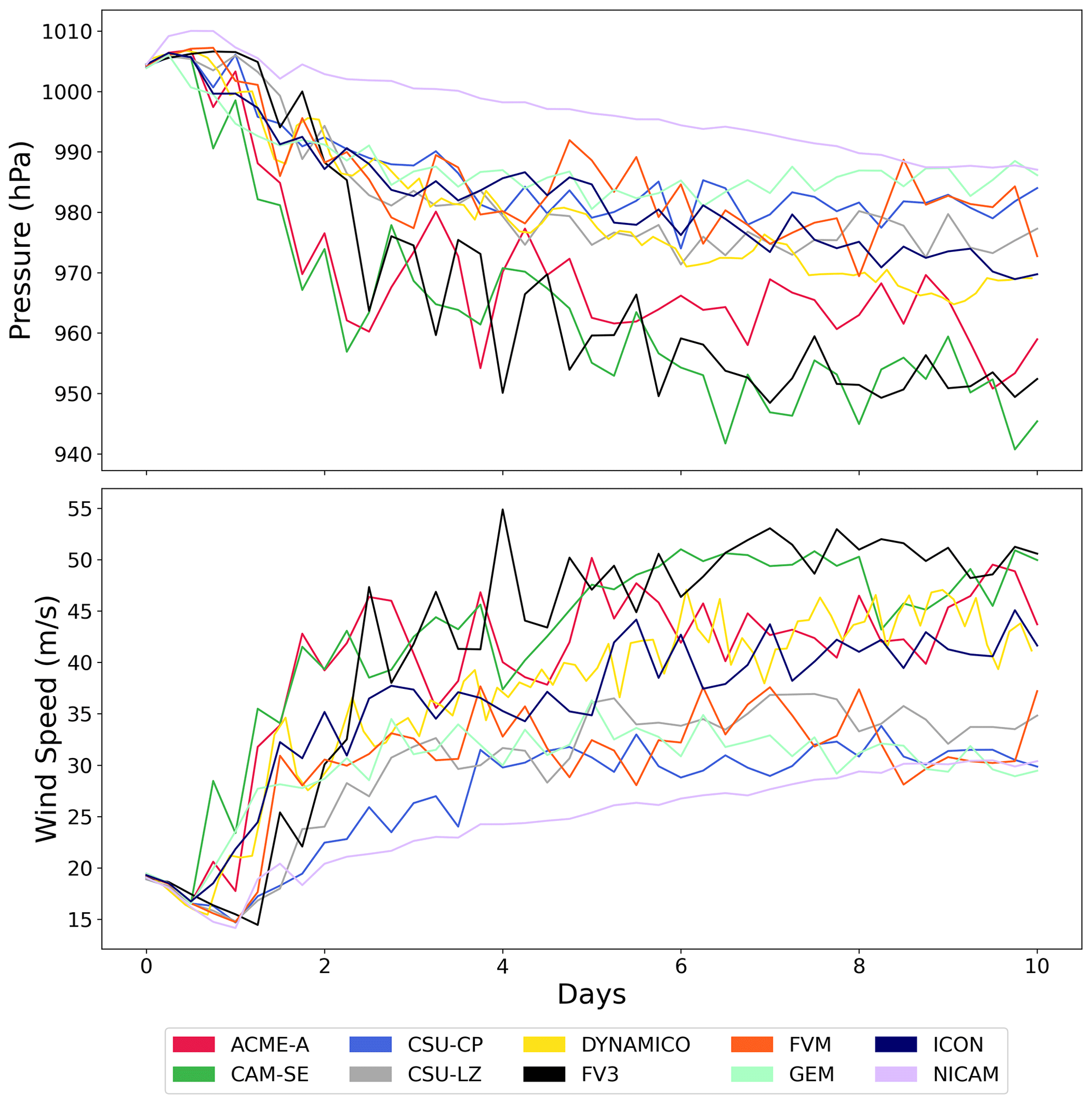
Figure 1 Evolution of MSP and MWS over the 10 d simulation period for the 50 km grid spacing.

The wind–pressure relationship within each TC was analyzed by plotting the corresponding MWS and MSP values at each time step. A second-order polynomial function was then fit using a least-squares method on each set of points. This method has been used in several prior studies, including Reed et al. (2015), where it was used to quantify the wind–pressure relationship in multiple CAM simulations and IBTrACS data; Knaff and Zehr (2007), where it was used to fit observational aircraft pressure data and best-track wind data; and Kossin (2015), where it was used to fit the wind–pressure relationship during eyewall replacement cycles seen in low-level aircraft reconnaissance data.

3 Results

The following section describes the results of the intercomparison with the intent of highlighting differences in the resulting TC behavior across the DCMIP2016 ensemble. Although various model details were briefly mentioned in Sect. 2.2 (and in more detail in Ullrich et al., 2017), this analysis will not try to attribute individual model characteristics as the reason for the differences in simulated TC behavior. Instead, we aim to provide an overview of the RJ TC test case results in DCMIP2016 and discern characteristics of model groups based on similar TC behavior or highlight differences between one or more models in certain areas. This form of analysis ultimately provides a catalog of solutions that serve as a benchmark for modeling groups to utilize in future work.

3.1 Time evolution of wind speed and pressure

The evolution of the MWS and the MSP is shown in Fig. 1. All MSP and MWS values are physically viable in the simulations, with MSP remaining above 940 hPa and MWS ranging from tropical storm strength to category 3 strength on the Saffir–Simpson scale. The MSP initially increases in all models, a sign of the weakening of the vortex, which has been seen in simple-physics simulations in Reed and Jablonowski (2012) and in more complex full-physics simulations in Reed and Jablonowski (2011c, 2012). All models then begin to intensify as the MSP decreases, and three model groups form shortly after day 2. NICAM retains the highest MSP, which decreases linearly throughout the remainder of the simulation. CSU-CP, CSU-LZ, DYNAMICO, GEM, FVM, and ICON MSP values decrease to between 970 and 990 hPa and vary within this range at subsequent time steps. The models increasingly diverge during days 7 to 10, and by day 9 NICAM enters this pressure range and becomes part of this model grouping. The MSP values of ACME-A, CAM-SE, and FV³ continue decreasing until approximately day 4, 1–2 d later than the previous group of models, and then generally remain in the 950 to 970 hPa range. These models all contain high variation in MSP changes compared to the other models, with differences in 5 hPa or above routinely seen at adjacent time steps.

Similarly, all models initially experience a decrease in their MWS during the first 1–2 d of the simulation, which quickly intensifies until around day 4, and enter a steady state for the remainder of the simulation. There are exceptions to this trend; for example, the MWS in NICAM linearly increases throughout the simulation period with little variation. The models again split into groups, in this case after day 5 of the simulation. CSU-CP, CSU-LZ, FVM, GEM, and NICAM tend to be less intense, with MWS values ranging between 25 and 35 m s⁻¹. The second group of models, ACME-A, CAM-SE, FV³, DYNAMICO, and ICON, have MWS values generally between 35 and 55 m s⁻¹ and are in some cases significantly more intense than the other set of models. Model groupings were not identical to those seen in MSP evolution since DYNAMICO and ICON are included in the higher-intensity group regarding MWS values. In all models except NICAM, the variability was approximately equal, with the majority of MWS changes in adjacent time steps being under 10 m s⁻¹ during the steady-state period.

3.2 Wind–pressure relationship

Figure 2 displays the MWS against the MSP at all time steps in the TC's evolution. The wind–pressure relationships of all the models were physically possible since the MSP and MWS were within the observed ranges of these variables. These ranges are seen in plots of observational data in Knaff and Zehr (2007) and Reed et al. (2015), which show that MSP has an approximate range of 870–1015 hPa and that MWS has an approximate range of 8–85 m s⁻¹. In all models, MWS increases as MSP decreases, and this increase is generally nonlinear, especially at high intensities. As in the analysis of the evolution of MSP and MWS, there are groupings of the models that display similar wind–pressure relationships, and these groupings tend to map to groupings seen in Fig. 1.

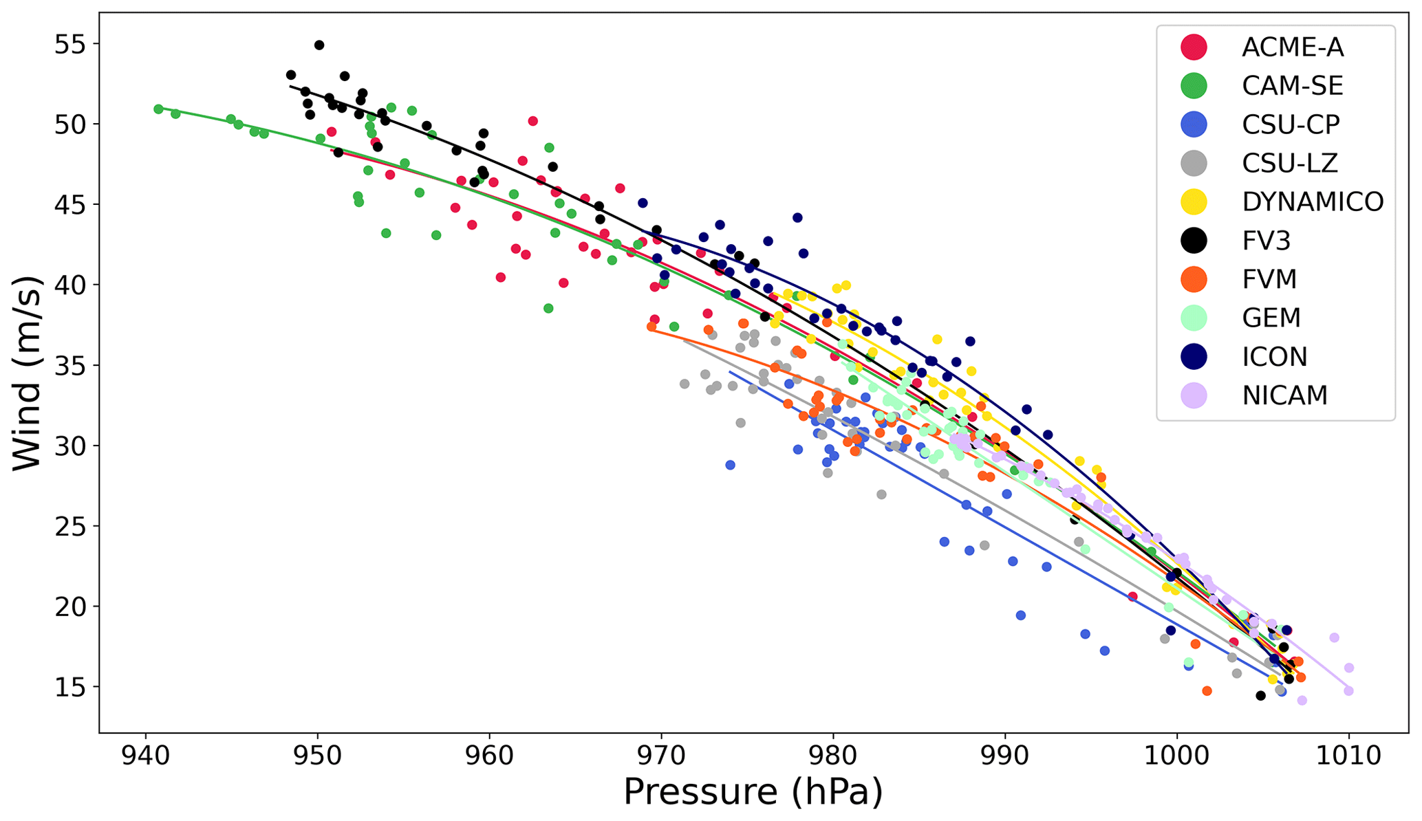
Figure 2 Wind–pressure relationship in the simulated TCs at all time steps for the 50 km grid spacing. MWS and MSP from Fig. 1 were used in this calculation. Second-order polynomial functions are fit using a least-squares method.

ACME-A, CAM-SE, and FV³ all have few points at low intensities, indicating how they quickly intensify in the first 1–2 d of the simulation. This intensification occurs with low variability, – that is, the fluctuation in points around the fitting curve – but high-intensity points tend to vary more. The next group of models, DYNAMICO, FVM, and ICON, contain members that were part of both the high-intensity and the low-intensity model groups in Fig. 1. The wind–pressure relationships of these models are similarly nonlinear with most of the points also occurring in the high-intensity region. In this case, the variability is more evenly distributed among the entire range. The final group of models, CSU-CP, CSU-LZ, GEM, and NICAM, have the lowest intensities and most-linear wind–pressure relationships, in part due to relatively weak intensities. NICAM has very little variability except in areas of low intensities, which was expected based on the smoothness of the evolution curves in Fig. 1.

3.3 Horizontal and vertical TC structure

The horizontal structure of the simulated TCs is analyzed using radial profiles of 1 km wind speed and surface pressure (Fig. 3), both of which were azimuthally averaged. The wind speed quickly increases with increasing radius until it reaches its maximum value of 25–50 m s⁻¹ depending on the model. For all models except GEM and NICAM, this maximum occurs at an approximate radius of 100 km. The maximum wind speed for GEM occurs slightly closer to the TC center, while NICAM's maximum wind speed occurs at a radius of approximately 200 km. After the radius of maximum wind speed, the wind speed decreases exponentially in all models, slowly approaching 0 m s⁻¹ at large radii. All models have wind speeds below 10 m s⁻¹ at radii greater than 600 km, behavior likely linked to the identical physical environment TCs are initialized in. The results shown here are similar to theoretical and observed azimuthally averaged surface wind radial profiles given in Chavas and Lin (2015) and Chavas et al. (2017). While the observed radial profiles in Chavas and Lin (2015) tend to have smaller radii of maximum wind speeds, the general structure of the radial profile is in agreement.

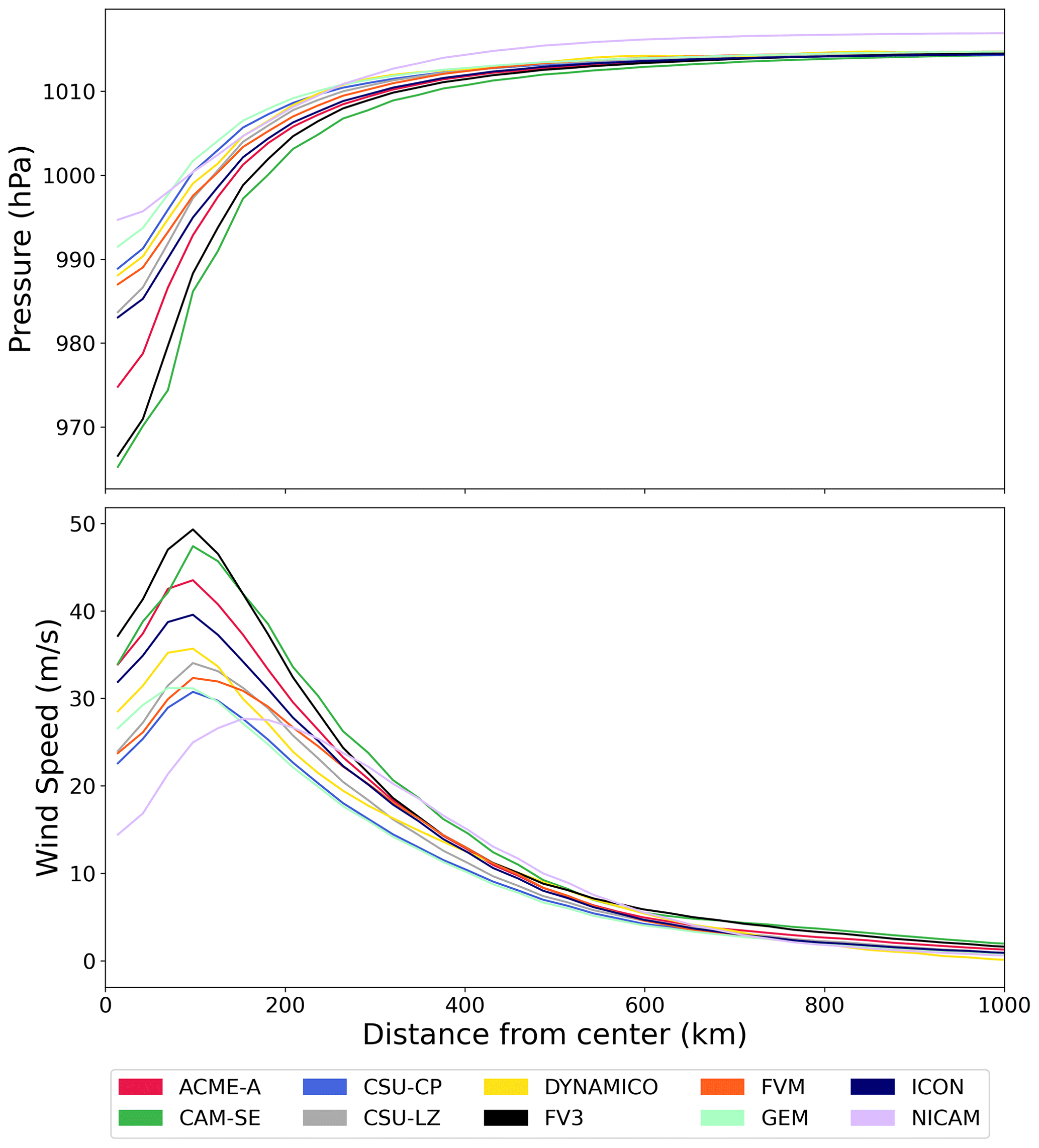
Figure 3 Radial profiles of 1 km wind speed and surface pressure averaged from days 4–10 of the 50 km simulation. Values in the radial profiles are azimuthally averaged.

MSP values range from approximately 965 to 995 hPa. The most intense models are again ACME-A, CAM-SE, and FV³, which have minimums in the 965–975 hPa range, while all other models have minimums in the 985–995 hPa range. The pressure values in all models then rapidly increase until an approximate radius of 200 km, after which they remain relatively constant and approach the background surface pressure value of 1015 hPa, which is consistent with Sect. 2.1.1 and the initialized environment. This behavior occurs in all models except NICAM, which plateaus at a pressure above 1015 hPa, possibly due to an initialization error. The radial surface pressure profiles in Chavas et al. (2017) have similar radial structure, indicating that the intermediate-complexity simulations produce behavior seen in more complex GCM simulations.

The 2D structure of the TC is analyzed using azimuthally averaged radial wind composites (Fig. 4). Starting from the TC center, the azimuthally averaged wind speeds quickly increase with increasing radius. The region of the most intense TC winds is generally centered around a 100 km radius, reaches a maximum altitude of 5–10 km, and has a maximum radial width of 100–200 km. There are some exceptions to this as NICAM's wind field has a flat top and no significant peak, while FV³ has a maximum altitude above 10 km. The most intense winds occur in ACME-A, CAM-SE, FV³, and to a lesser extent ICON, where wind speeds are greater than 40 m s⁻¹ compared to 30–35 m s⁻¹ for the remaining models. Similar results are seen in more complex GCM simulations analyzed in Moon et al. (2020), where the wind fields of simulated TCs in GCMs have similar 2D structure in their most intense winds.

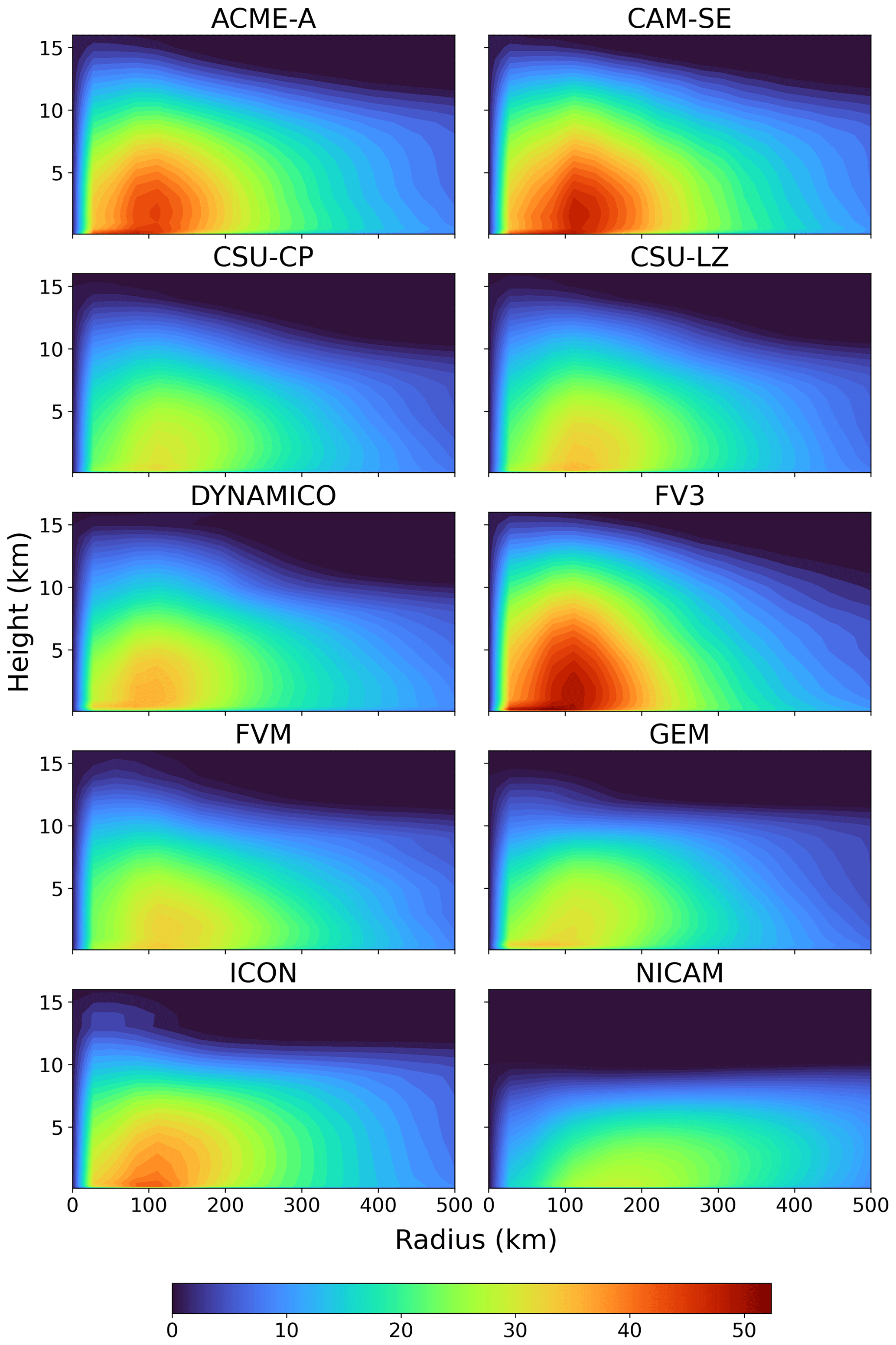
Figure 4 Azimuthally averaged vertical wind composite of the simulated TCs from days 4–10 of the 50 km simulation.

Based on the structural properties of the wind composites, the models can be placed into similar groupings as seen in Figs. 1–3. The most intense models are again ACME-A, CAM-SE, and FV³. DYNAMICO and ICON have regions of strong winds; however, they did not form at the same altitude, width, shape, or intensity as the previous three models. CSU-CP, CSU-LZ, FVM, and GEM only show small signs of intense wind formation and are largely unable to simulate winds above 35 m s⁻¹ in the wind composite.

3.4 Impact of finer grid spacing

The previous analysis is now repeated at 25 km grid spacing for participating models (Table 5). The time evolution of MSP and MWS is first examined and results are seen in Fig. 5. For both MWS and MSP, the evolution largely resembles the coarser grid spacing case in Fig. 1. There is a period of significant intensification in the first 4 d followed by a steady-state time period. In almost all cases, the 25 km simulations are more intense than their 50 km counterparts, and the most intense models in the 50 km simulation are also the most intense in the 25 km simulation. ACME-A and CAM-SE are the most intense models in both grid spacings, with their MWS increasing from 40–50 to 50–60 m s⁻¹ and their MSP decreasing from approximately 950–970 to 920–940 hPa with the change to 25 km grid spacing. An increase in TC intensity in CAM with finer grid spacing is shown in several studies, including Reed and Jablonowski (2011a, b) and Reed et al. (2012), and is likely related to implicit and explicit diffusion becoming weaker (Jablonowski and Williamson, 2011). FVM and GEM are again models with intermediate intensity, and FVM tends to have a larger increase in intensity than GEM by approximately 5 m s⁻¹ for MWS and 15 hPa for MSP. NICAM is unique in this analysis because of its substantial increase in intensity, upwards of 15 m s⁻¹ for MWS and 30 hPa for MSP, but these large changes only occur during days 2–8 of the simulation.

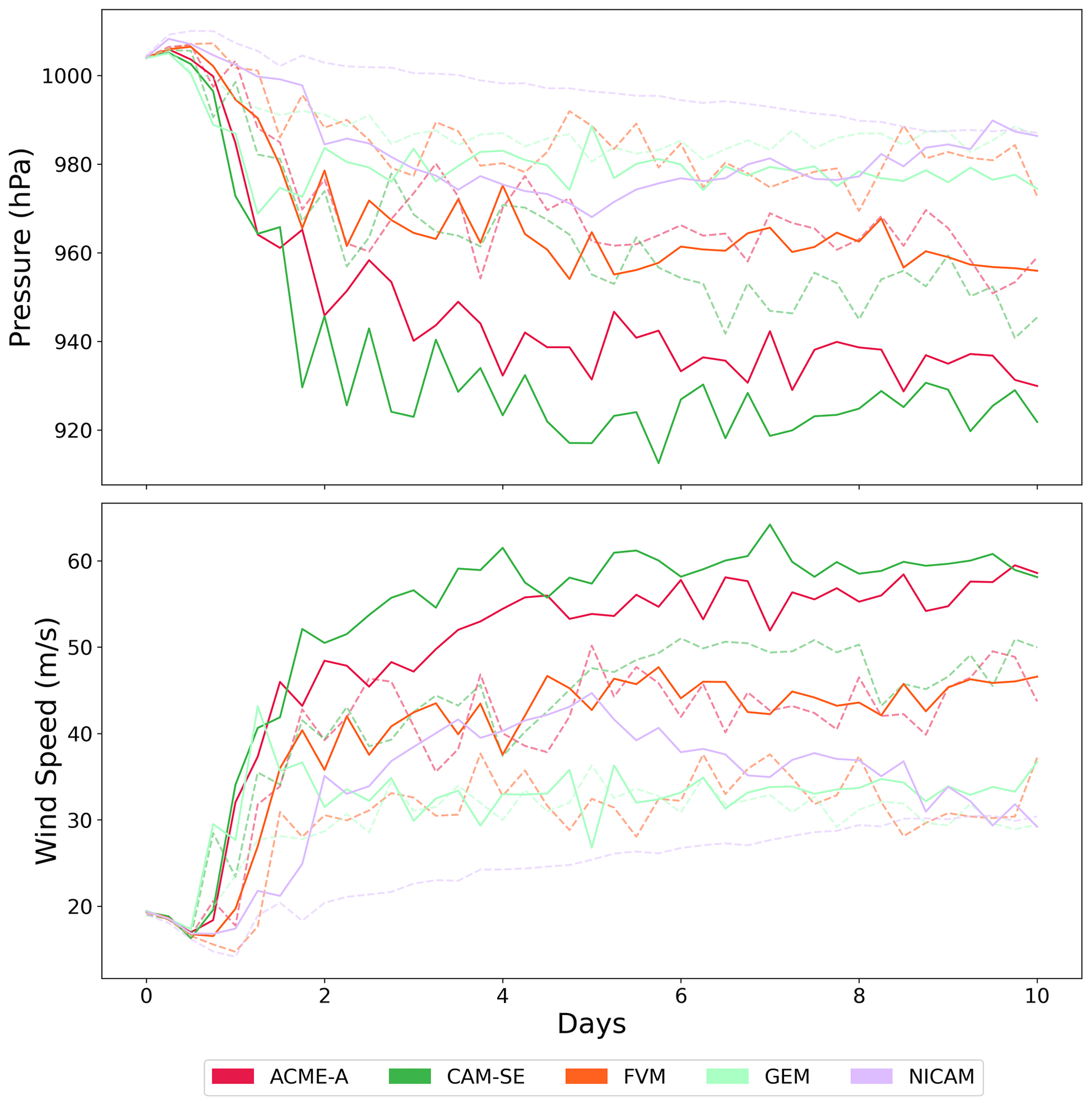
Figure 5 Evolution of MSP and MWS over the 10 d simulation period. Grid spacings of 50 km (dashed line) and 25 km (solid line) are shown for participating models.

The wind–pressure relationships (Fig. 6) have larger MSP and MWS ranges for all models, which was expected due to larger intensities at 25 km grid spacing. As in the 50 km simulations, most of these relationships are nonlinear since the rate of increase in MWS tends to decrease at lower MSP. Additionally, a majority of the points occur at the high-intensity region, as before, due to the longer period of the simulation spent by the TC at high intensity. The MSP and MWS values seen in this analysis are within observed ranges for TCs, reaching up to category 4 on the Saffir–Simpson scale.

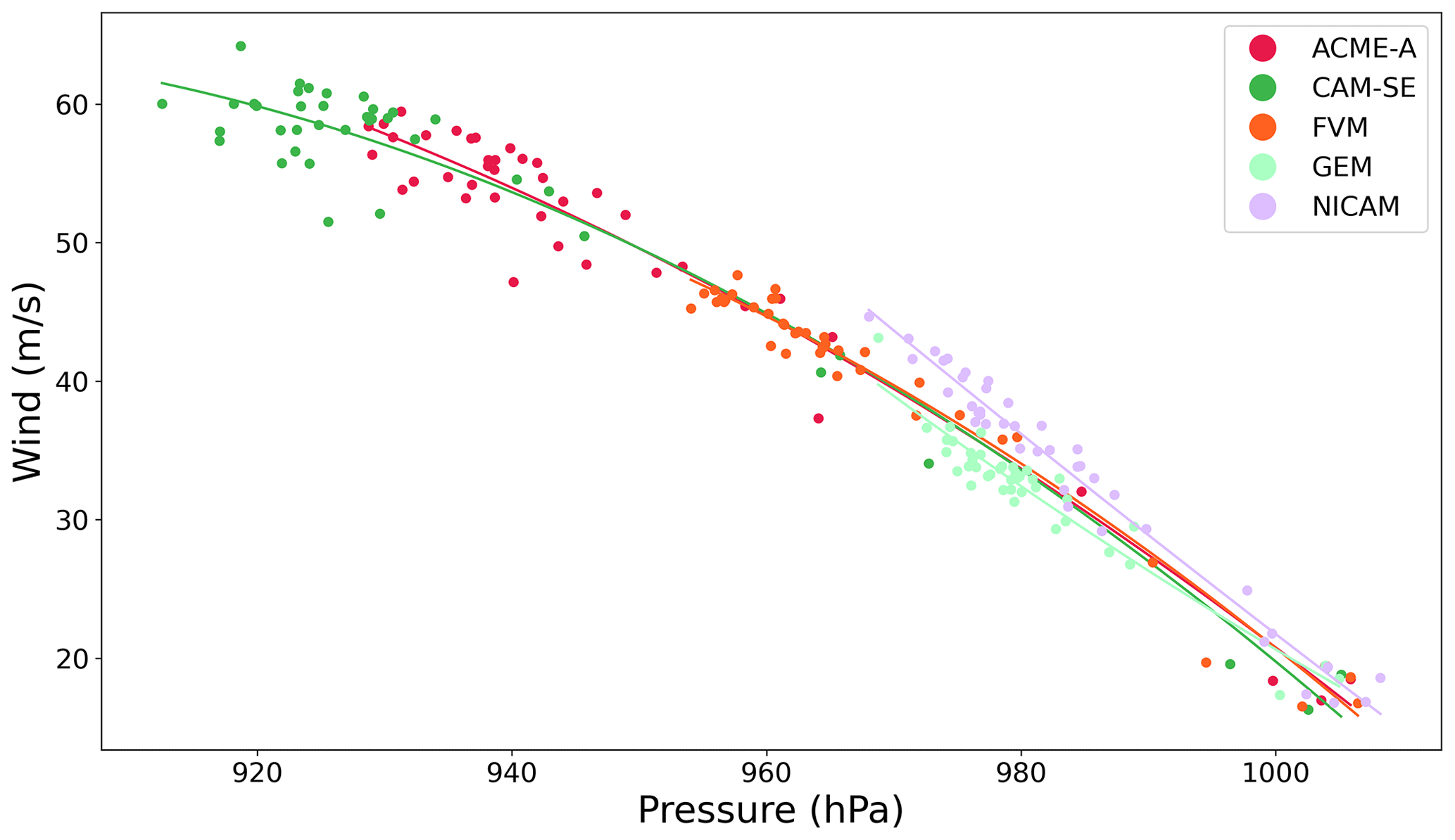
Figure 6 Wind–pressure relationship in the simulated TCs at all time steps for 25 km simulations of participating models.

Radial profiles of 1 km wind speed and surface pressure (Fig. 7) are used to determine how the TC horizontal structure changes at finer grid spacing. As in the coarser grid spacing simulations, the wind speed increases rapidly with radius until it reaches a maximum and subsequently decreases exponentially and reaches an asymptotic value of 0 m s⁻¹. At finer grid spacing, this maximum wind speed value occurs at a smaller radius, approximately 50 km compared to 100 km, and has a larger magnitude. All models significantly increase in intensity, often by 10 m s⁻¹ or greater, in the core region.

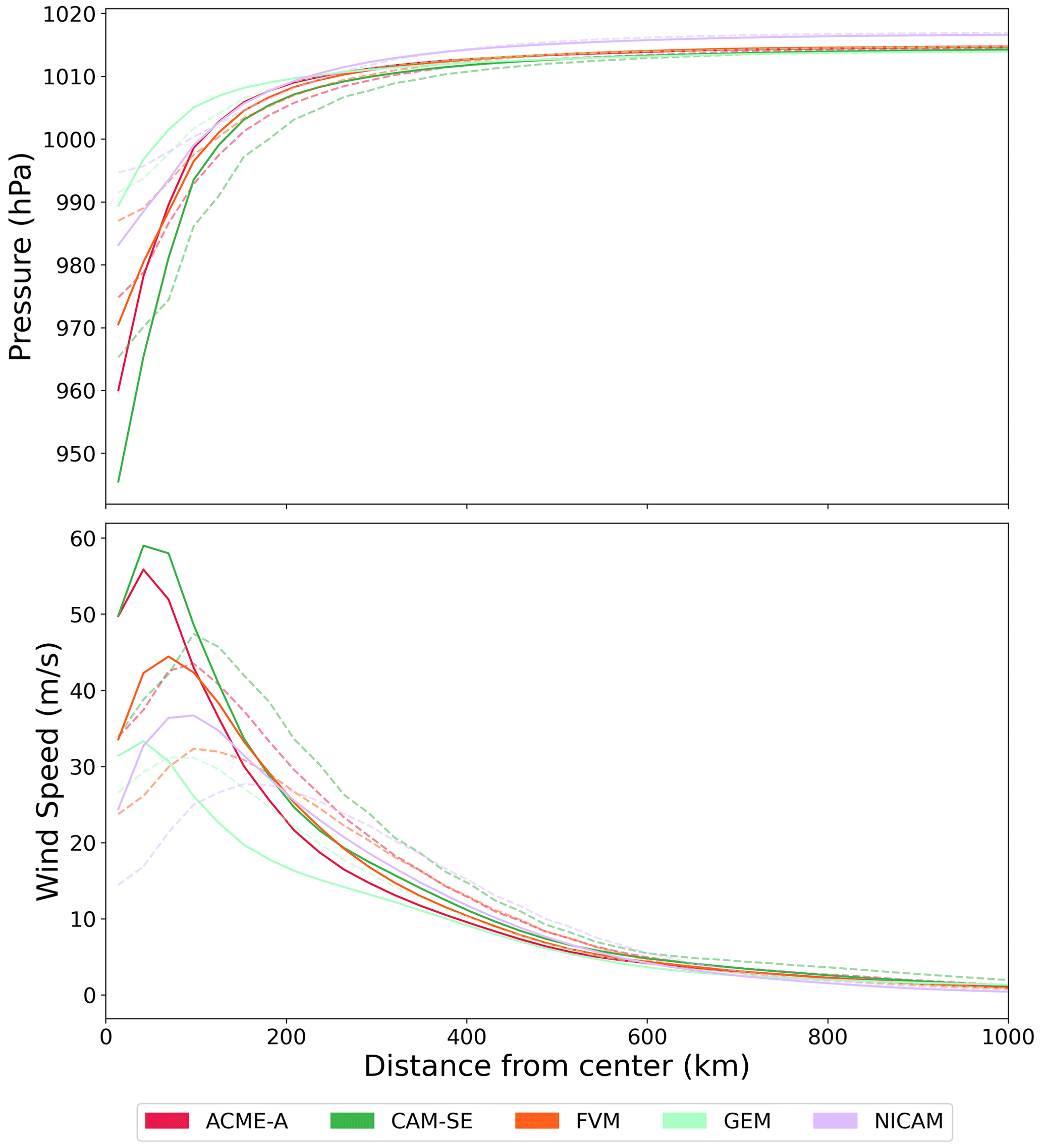
Figure 7 Radial 1 km wind speed and surface pressure profiles averaged from days 4–10 of the simulation. Values in the radial profiles are azimuthally averaged. Values of 50 km (dashed line) and 25 km (solid line) are shown for participating models.

Surface pressure radial profiles at finer grid spacing also have similarities to those at coarser grid spacing. In both cases, the minimum surface pressure values at the center rapidly increase at relatively small radii, and the rate of increase eventually slows and surface pressure reaches the prescribed value (Sect. 2.1.1) at large radii. The minimum pressure values decrease in all models by 10–20 hPa. At 25 km, the surface pressure profiles, similarly to the wind profiles, are more compact since they tend to plateau at a smaller radius, which is consistent with the larger magnitude and smaller radius of maximum winds. Results converge at radii greater than 400 km for all models.

As with the previous quantities, grid spacing has an impact on the wind composites (Fig. 8). The overall 2D structure of the 25 km TCs remains similar to that of the 50 km TCs, but there are key differences. As before, there is a narrow region of weak winds by the TC center at all heights followed by a stronger wind field that extends to a radius of approximately 300 km and a height of exactly or above 10 km. In ACME-A and CAM-SE, the most intense models, there is a region of intense winds that is more compact at 25 km grid spacing, which extends to around a 100 km radius compared to a 200 km radius in the 50 km simulations. This region contains stronger winds that are routinely greater than 50 m s⁻¹. This decrease in the radius of maximum winds is seen in the remaining models as there is a 50–100 km decrease in GEM, FVM, and NICAM. In particular, GEM becomes much more compact, especially at altitudes higher than 5 km, and has a profile with a different overall shape. Wind composites also become more compact at finer grid spacing in the more complex GCM simulations analyzed in Moon et al. (2020).

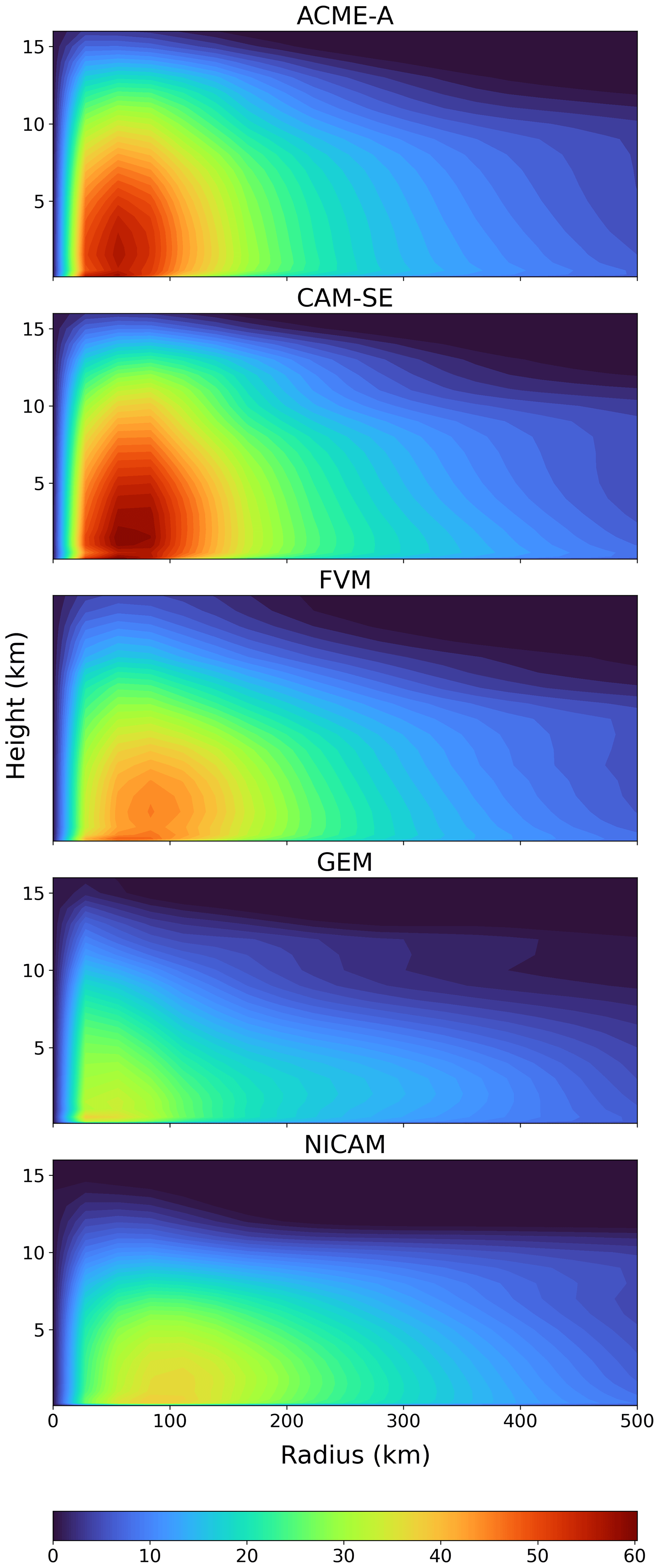
Figure 8 Azimuthally averaged vertical wind composite of the simulated TCs from days 4–10 of the 25 km simulation.

4 Conclusions

The RJ TC test case results demonstrate that solutions vary between DCMIP2016 models with different dynamical cores and identical simple-physics parameterization packages and physical environments, building on the work of Reed and Jablonowski (2012). Most participating GCMs produce a TC with similar MWS and MSP evolutions, wind–pressure relationship, radial profiles of wind and pressure, and wind composites; however, there are important differences between them. Certain models were more intense overall, and that is reflected in their MWS, MSP, and horizontal and vertical structures. These intensity differences are likely tied to the effective resolution of the dynamical core, which is the shortest wavelength which is accurately simulated in the model (Kent et al., 2014). GCMs also have relatively large intensity spread, possibly due to thermodynamic structures (Moon et al., 2020) or dynamical core choice (Reed et al., 2015). Similarly, numerical weather prediction (NWP) models have large TC intensity root-mean-square errors, often on the order of 2.5–8 m s⁻¹, depending on lead time (Zhang et al., 2023), although they are smaller in magnitude than the intensity spread seen in this study. Additionally, the physics–dynamics coupling is a further source of uncertainty in this test case (Gross et al., 2018). TC behavior among participating models also changes when the horizontal grid spacing becomes finer. TCs simulated at 25 km grid spacing tend to be more intense and compact than those simulated at 50 km grid spacing. Models that produced the most intense TCs at 50 km also produced the most intense TCs at 25 km, indicating that some differences between the models are preserved at finer grid spacing. In the intercomparison, NICAM was an outlier, possibly due to an initialization error. It is evident that the dynamical core has an essential role in determining the resulting TC behavior in GCMs. While the impact of the dynamical core has been investigated thoroughly in studies including one or two models, the intercomparison of a larger group of models illustrates this role and related sensitivity to horizontal grid spacing. The dynamical core choice should be carefully considered in the GCM development process, and more work can be done to better quantify its effects when all other parameters are held constant. The goal of this study is to present a general intercomparison of TC behavior among a grouping of models that differed in dynamical core. In doing so, this work provides a library of solutions that can serve as a benchmark for modeling groups to compare with during the model development process, similar to other non-TC-focused intercomparison efforts (e.g. Blackburn et al., 2013; Zarzycki et al., 2019). This is especially important since the RJ TC test case and other DCMIP2016 test cases are widely used in the community and some test cases are readily available in CESM. Future work could examine differences between specific dynamical core characteristics and how those differences impact TC simulation in intermediate-complexity simulations.