cloudbandPy 1.0: an automated algorithm for the detection of tropical–extratropical cloud bands

Persistent and organized convective cloud systems that arise in convergence zones can lead to the formation of synoptic cloud bands extending from the tropics to the extratropics. These cloud bands are responsible for heavy precipitation and are often a combination of tropical intrusions of extratropical Rossby waves and processes originating from the tropics. Detecting these cloud bands presents a valuable opportunity to enhance our understanding of the variability of these systems and the underlying processes that govern their behavior and that connect the tropics and the extratropics. This paper presents a new atmospheric cloud band detection method based on outgoing longwave radiation using computer vision techniques, which offers enhanced capabilities to identify long cloud bands across diverse gridded datasets and variables. The method is specifically designed to detect extended tropical–extratropical convective cloud bands, ensuring accurate identification and analysis of these dynamic atmospheric features in convergence zones. The code allows for easy configuration and adaptation of the algorithm to meet specific research needs. The method handles cloud band merging and splitting, which allows for an understanding of the life cycle of cloud bands and their climatology. This algorithm lays the groundwork for improving our understanding of the large-scale processes that are involved in the formation and life cycle of cloud bands and the connections between tropical and extratropical regions as well as evaluating the differences in cloud band types between different ocean basins.

1 Introduction

Convergence zones can be described as broad bands of persistent, quasi-stationary convectively active clouds, which are aligned from northwest to southeast and from southwest to northeast in the Southern and Northern Hemisphere, respectively. They typically occur throughout the respective wet season. The water and energy cycle within these convergence zones is strongly modulated by individual storm events that are embedded in the synoptic circulation, similar to other convective regions (Rickenbach and Rutledge, 1998; Schumacher and Houze, 2003; Roca et al., 2010, 2014). These individual storm events play a crucial role in shaping the distribution and intensity of precipitation, affecting the overall hydrological and atmospheric dynamics within the convergence zone. There are four tropical convergence zones, which are the Baiu frontal zone (BFZ), which is considered here jointly with the Meiyu frontal zone over East Asia (Kodama, 1992, 1993; Li et al., 2018), the South Atlantic convergence zone (SACZ) (Carvalho et al., 2004; Villela, 2017), the South Indian convergence zone (SICZ) (Cook, 2000), and the South Pacific Convergence Zone (SPCZ), which is the most vast and intense (Vincent, 1994; Matthews, 2012; Brown et al., 2020). The convergence zones are formed by low-level wind convergence, which causes an accumulation of moist air and eventually leads to an upward movement of air, convective activity, and intense rainfall (Streten, 1973). As convective storms progress within the convergence zone, they intensify moisture convergence, fostering heightened cloud formation and precipitation (Hudson, 1971; Houze, 1997; Tsuji et al., 2021). The synoptic circulation provides the large-scale framework for these individual storm events and influences the spatial organization and evolution of the storms within the convergence zone.

The SPCZ is the primary region where persistent deep tropical convection frequently merges with troughs from the midlatitude circulation. Its largest extent is observed during austral summer (Vincent, 1994). Convergence zones allow for the organization of mesoscale convective systems (MCSs) (Matthews et al., 1996; Takahashi and Battisti, 2007; Oueslati and Bellon, 2013), which consist of an ensemble of cumulonimbus towers and anvils that become organized on a scale larger than the individual convective core (Houze, 2004) and that form long, narrow bands that extend from the tropics to the subtropics with a northwest–southeast orientation in the Southern Hemisphere and a southwest–northeast orientation in the Northern Hemisphere (sometimes referred to as a diagonal tilt). Given that the cloud bands over the SPCZ are a significant contributor to precipitation, especially on Pacific islands, it is crucial to document them in order to gain a better understanding of the water and energy cycle.

Atmospheric feature extraction and tracking can aid in this effort to identify cloud bands by creating a reduced dataset that allows for more efficient visualization and statistical evaluation of cloud bands. Originating from image processing and computer vision Zucker (1976), this technique has proven to be a valuable tool for identifying and analyzing features of interest in various fields. In the extratropics, atmospheric feature detection has been successfully applied to study midlatitude cyclones (Ulbrich et al., 2009), jet stream features (Limbach et al., 2012), and extreme precipitation events associated with potential vorticity streamers and integrated water vapor transport structures (de Vries et al., 2018). Post et al. (2003) and Limbach et al. (2012) provide comprehensive overviews of conceptual views on feature identification and tracking in atmospheric sciences.

In addition to their application in the extratropics, image processing techniques have also been instrumental in the detection of organized convective cloud systems. These cloud systems can be identified using satellite data at a global scale or using measures such as infrared brightness temperature (Fiolleau and Roca, 2013; Roca et al., 2014; Huang et al., 2018; Laing and Michael Fritsch, 1997; Williams and Houze, 1987) or radar reflectivity (Nesbitt et al., 2006; Kummerow et al., 2011; Houze et al., 2015) by combining brightness temperature and precipitation from the Global Precipitation Measurement dataset (Feng et al., 2021, 2023). These studies focused on the life cycle of MCSs.

Another proxy for deep convection is the outgoing longwave radiation (OLR). Deep convective clouds are usually identified by their cold cloud tops, which emit low OLR values. These clouds possess a dense and vertically extended structure, leading to reduced emission of longwave radiation. Consequently, low OLR values often signify the presence of high, thick clouds, including deep convective clouds. OLR has been used to study organization of convection (Holloway and Woolnough, 2016), as well as energy balance and tropical convection (Hartmann et al., 2001), to estimate deep convection (Waliser et al., 1993; Zhang et al., 2017), or to study the link between convective clouds, anvils, and cirrus clouds (Massie et al., 2002; Sokol and Hartmann, 2020).

Larger cloud systems, such as tropical–extratropical cloud bands, are often detected using satellite imagery or reanalysis data using OLR thresholding, i.e., by dividing OLR into two groups with low and high values, respectively, to distinguish different clouds according to their radiation characteristics Kodama (1992, 1993). Low OLR values typically indicate the presence of convective or cirrus clouds, while high OLR values are associated with regions where the atmosphere is relatively clear of clouds or where the cloud cover consists of thin or (thick) low-level clouds. While OLR detection may not achieve the same accuracy as methods using brightness temperature and precipitation features, it remains a valuable tool for identifying these large-scale systems. This is especially true for quasi-stationary tropical–extratropical cloud bands consisting of several MCSs, where the use of precipitation features and high-frequency data may not be as relevant. More recent work has focused on the detection of cloud bands over the SACZ (Zilli and Hart, 2021; Rosa et al., 2020) and extratropical cloud bands over the SICZ (Hart et al., 2012, 2018).

Despite the different detection methods available for tropical–extratropical cloud bands, all cloud band studies focus on the subtropical part of the cloud bands. Most of the available open-source tools for cloud band detection are tailored for the subtropics, do not treat merging and splitting of cloud bands (which allows for a better understanding of the large-scale processes at play), are not optimized to work with different data, and have thresholds that are dependent on the specific dataset.

This study aims to overcome these shortcomings by introducing a user-friendly Python software package, built on a supported Python version, designed to detect and track the life cycle of extended tropical–extratropical cloud bands. Specifically, the software package tracks the inheritance of cloud bands, providing a better understanding of the representation of a cloud band's life cycle. The algorithm is applicable to various types of gridded data and can operate at different temporal and spatial scales. It explicitly handles the merging and splitting of features and includes visualization and analysis of detected cloud bands. It also includes visualization and analysis tools for the detected cloud bands. The goal of this paper is to describe this algorithm and to demonstrate its capabilities with examples applied to reanalysis data and to identify the limitations of thresholding image-segmentation methods to study these large-scale cloud bands. The algorithm serves to connect large-scale processes that link the tropics to the extratropics, with cloud bands acting as a proxy for further studies.

2 Data and methods

2.1 Dataset

We utilize the ERA5 global reanalysis dataset (Hersbach et al., 2020) from the European Centre for Medium-Range Weather Forecasts (ECMWF) as input data for our cloud band detection algorithm. This dataset provides hourly estimates of a large number of atmospheric, land, and oceanic climate variables on a 30 km grid and at 137 vertical levels. In this study, cloud bands are detected from 1959 to 2021 using ERA5 OLR data at 3 h intervals regridded to a regular latitude–longitude grid of 0.5° at a global scale.

We opted for ERA5 over satellite retrievals due to its convenience and various advantages. Our primary goal is to seamlessly integrate this algorithm into models, leveraging the widespread availability of OLR, which is more commonly used in atmospheric models than black-body temperatures at the cloud top or brightness temperatures, making this algorithm particularly useful in combination with models. ERA5 has the benefit of high temporal and fine horizontal resolution and therefore serves as an ideal source for our study. While ERA5 demonstrates commendable performance in representing tropical mean values of OLR, we acknowledge certain limitations, notably its tendency to underestimate cloud radiative effects. However, the distributions of longwave and shortwave radiation (radiation emitted by particles in the atmosphere and land surfaces and solar radiation received and reflected by the Earth's surface, respectively), as well as total cloud radiative effects at the top of the atmosphere in ERA5, consistently align with observed values. This consistency distinguishes ERA5 from other reanalyses (Wright et al., 2020) and underscores its reliability in our cloud band detection methodology.

2.2 Cloud band identification

Low OLR values generally correspond to the cold cloud shields of convective systems, which include the core of the convective system and its anvil. In this study, the algorithm uses OLR data to identify tropical–extratropical diagonal cloud bands associated with deep convective cloud systems. The algorithm includes a threshold-based segmentation and utilizes a morphological approach, which modifies the shape of objects in an image and extracts valuable information, such as their geometric characteristics. Segmentation refers to dividing the image into regions of pixels based on the OLR threshold and has been used in other studies such as in SACZ or SICZ automated detection algorithms (Hart et al., 2012, 2018; Rosa et al., 2020). Our method of tracking the time dependency of OLR associated with cloud bands takes into account the full life cycle of cloud bands. In addition, applying the method globally and across a wide range of latitudes (from the tropics to the extratropics) allows us to extend the cloud band climatology to a global scale, enabling a comparison between different basins and also highlighting the limitations of the tool presented here.

We apply the basic workflow of image data analysis to OLR data, which includes smoothing, binarization of the image, setting a threshold, applying morphological operations, and labeling. Version 3 of Python is used for all steps. Figure 1 presents a schematic flowchart detailing the step-by-step process of the cloud band identification developed in this study, which is subsequently explained in detail.

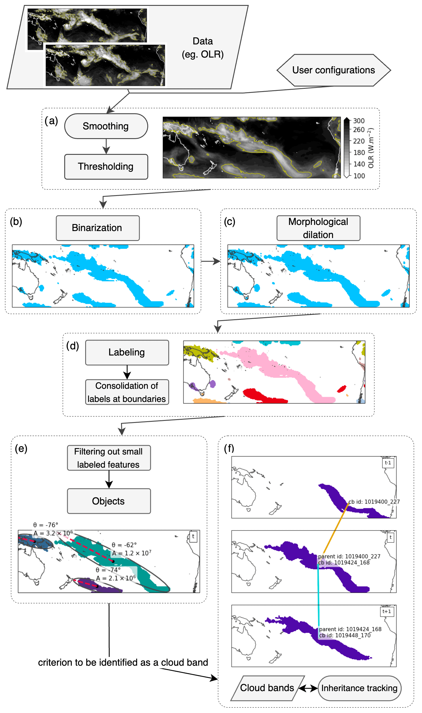
Figure 1 Case study example of the cloud band identification processing steps over the South Pacific Ocean. Data shown are snapshots of OLR on 18 April 2016 at 03:00 and 06:00 UTC. (a) Daily mean OLR data in shading and 210 W m⁻² isocontour in yellow, (b) binarization, (c) morphological dilation, (d) connected component labeling with different colors indicating distinct identified features, (e) cloud systems with a size below a threshold value removed and geometrical properties calculated to filter tropical–extratropical cloud bands, (f) cloud band after filtering. The evolution of each cloud band is tracked between two consecutive time steps (see Sect. 2.4).

First, we calculate the daily mean of the 3-hourly OLR data (Fig. 1a). This average is used as the smoothing procedure that prevents over-segmentation of cloud systems; i.e., temporal smoothing increases the connectivity between low-OLR regions. Such over-segmentation usually occurs at the early stage of cloud band formation and at its last stage before splitting (see Sect. 2.4) or disappearance, when convective systems start to organize. Instead of using the temporal smoothing employed here, a spatial box smoothing may be needed when using different periods and may have to be adjusted for datasets of different temporal and/or horizontal resolution.

Secondly, a threshold is used to differentiate regions of low and high OLR values through binarization of the data (Fig. 1a, b). Choosing an appropriate value for thresholding images can be challenging. The main problem with thresholding is that it considers only the intensity for each single pixel, but not any relationships between the pixels. Following Massie et al. (2002) with respect to the distribution of tropical cirrus clouds associated with deep convective anvils and multiple sensitivity tests (see Appendix B), contiguous areas with smoothed OLR below values of 210 W m⁻² are identified here as distinct cloud systems (Fig. 1a). This threshold can be adjusted by the user. The limitations of using thresholding methods are described in the “Discussion and conclusion” section.

The above threshold is chosen for two reasons: the first reason is that the cloud band systems we want to identify are mainly convective and areas of frequent convection are often accompanied by a high occurrence of cirrus clouds (Sassen et al., 2009; Schoeberl et al., 2019; Nugent et al., 2022), which have OLR values below this threshold. Moreover we want to take into consideration anvils from deep convective clouds. The second reason is that we aim to prevent convective cloud systems, extending from the tropics to the extratropics, from forming a single region of low OLR values with upper-tropospheric cold clouds from midlatitudes and polar regions that extend over large areas.

Next, each cloud system undergoes a morphological dilation (Fig. 1c), adding pixels to the boundaries of each object in an image. Region growing allows us to merge clouds that occupy neighboring pixels and can prevent the subsequent labeling step from separating clouds that could be part of a single cloud band.

As a next step, all cloud systems are labeled using an eight-connected-components labeling method (Fig. 1d). Connectivity refers to the relationship between pixels and their neighbors, which can form objects or groups. Here, a pixel is considered to be connected to its eight neighbors. The labeling process involves iterating over all pixels in the image and assigning labels to connected objects. In the case of global cloud band identification, all labeled systems that intersect the longitudinal boundaries of the domain are consolidated by merging labeled features that connect through image boundaries. The labeled systems are treated as image-like arrays, allowing for measuring properties that are not dependent on the spatial resolution or the projection of the input data. To speed up the last step of the algorithm, smaller cloud systems are filtered out (Fig. 1e), where cloud systems below the threshold of 10⁵ km² are subsequently excluded. This threshold value is comparable to that of an organized convective system, which typically has an area of 10⁴ km² or larger (Roca and Ramanathan, 2000; Houze, 2004). To ensure that cloud systems are not excessively removed from the labeled systems, we visually examine a wide selection of time steps and values to determine a suitable area threshold.

Finally, each identified feature is transformed into an object. For each object, its geometric properties are calculated by drawing an ellipse around it. These geometric properties include the object's orientation (that is, the tilt of a cloud band with respect to the latitude–longitude grid) measured from the ellipse's centroid location and the orientation of its major axis (Fig. 1e). These geometric properties are then saved in each cloud band object. These properties are then utilized to filter out cloud bands from any other labeled features. Specifically, in this study, we define a tropical–extratropical diagonal cloud band as a cloud system with the following properties.

1. Its major axis has to exhibit an orientation between −5 and −90° in the Southern Hemisphere and between 5 and 90° in the Northern Hemisphere. Cloud bands without a strong enough latitudinal tilt, i.e., with an orientation along a latitude circle, are filtered out to prevent labeling cloud systems belonging, for example, to the Intertropical Convergence Zone (ITCZ) as a diagonal cloud band.

2. Each cloud band must cross 23.5° north or south, which defines the extent of the tropics. By doing so, we assume that cloud bands must have a minimal extent and must cover tropical and extratropical regions. Furthermore, for cloud bands to have a minimal extent, their northernmost and southernmost latitudes have to lie equatorward of 20° S and poleward of 27° S, respectively, in the Southern Hemisphere and equatorward of 20° N and poleward of 27° N, respectively, in the Northern Hemisphere. While these criteria are somewhat subjective, they are implemented to establish a baseline minimal extent. Users have the flexibility to adjust these values based on their preferences and requirements.

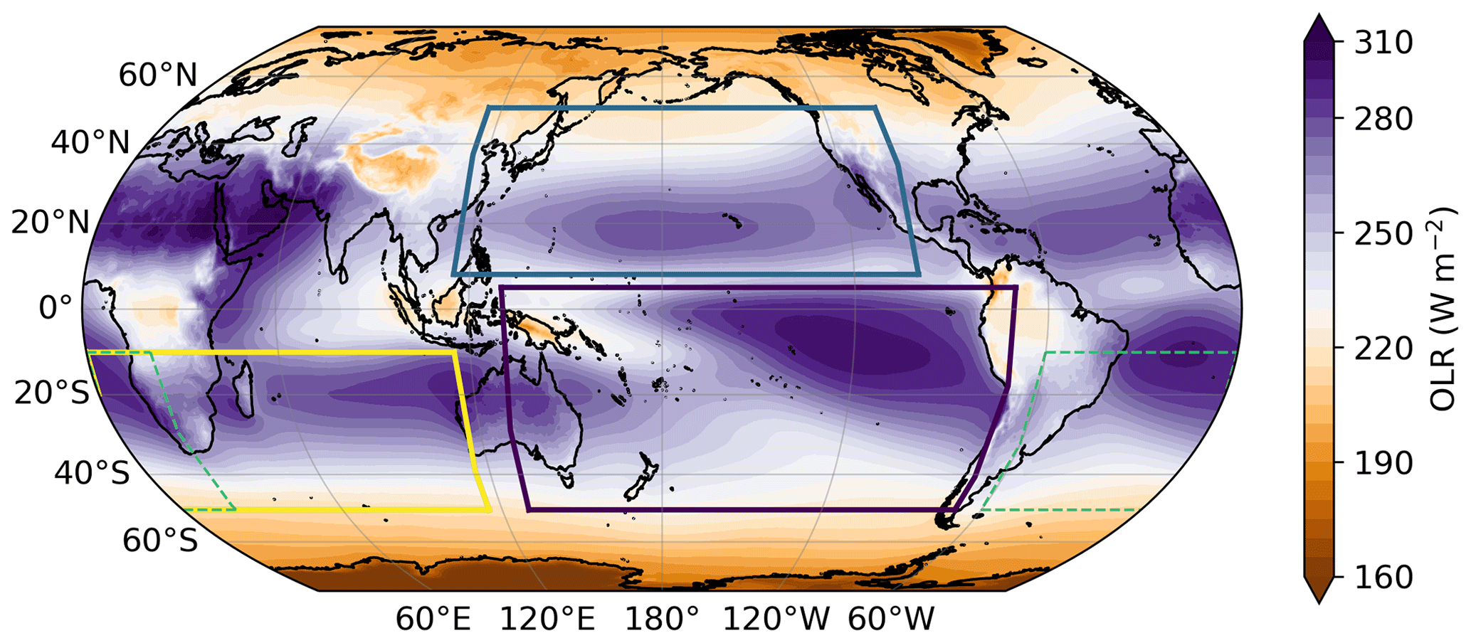
Figure 2 Average OLR (in W m⁻²) from 1959 to 2021 from ERA5 data. The rectangles correspond to the domains used in this study.

2.3 Domains of detection and limitations of a threshold-based detection

Although the detection workflow here is initially designed for the South Pacific Ocean and tested in both hemispheres, it is advisable to establish a specific domain for each basin based on the prevailing processes. This is particularly relevant for the detection of cloud bands over convergence zones, for which the workflow is specifically developed. Since the method is based on an OLR threshold, all regions covered by cold clouds can influence the identification and lead to a false identification of cloud bands by merging actual cloud bands with other cloud cover types (from the midlatitudes or from the ITCZ), despite the orientation criterion.

Moreover, low OLR values of cold clouds located over high-altitude terrains such as the Tibetan plateau (Su et al., 2000) may connect with other low-OLR regions emerging from the South Asian monsoon (Fig. 3a) and from the BFZ. Another example of erroneous detection is the presence of low OLR values above the Andes and the Bolivian high, which can connect cloud systems from the ITCZ with clouds from the SACZ (Lenters and Cook, 1997; Villela, 2017) (blue contour in Fig. 3b). Additionally, since the SPCZ may be seen as an extension of the ITCZ, the algorithm may identify the elongated region of low OLR values as a cloud band, influenced by the cloud orientation above the SPCZ (yellow contour in Fig. 3b). In such cases, the presence of diagonal cloud bands may be an artifact of the algorithm. Therefore, it is crucial to exercise caution when interpreting cloud band detection over these regions.

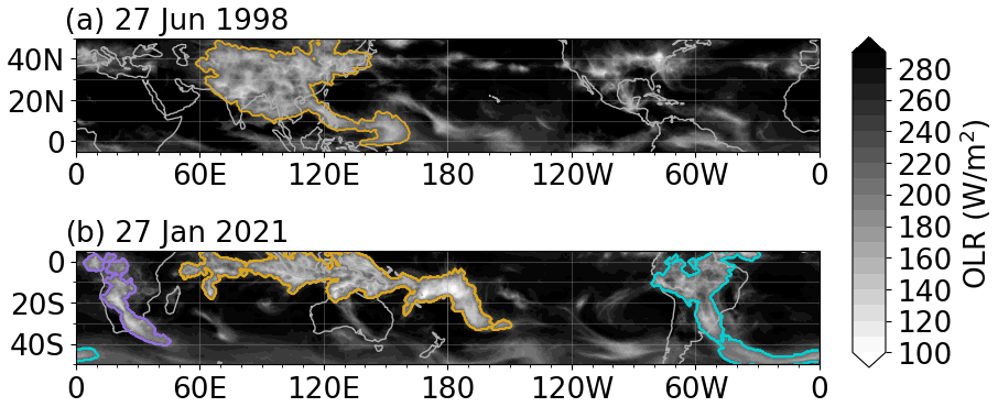
Figure 3 Illustration of problematic cloud band detection on (a) 27 June 1998 and (b) 27 January 2021, highlighting the significance of setting domains based on convergence zones. Shading corresponds to OLR data and colored contours represent detected cloud bands.

A guideline would be to define specific domains based on a climatology of OLR, as shown in Fig. 2. In this figure, we suggest four domains that encompass the four convergence zones. It is worth noting that the North Atlantic basin is not included in the selection as it does not exhibit a distinct convergence zone. The domains will be subsequently referred to by the names of the respective ocean basins. The North Pacific domain (115° E, 100° W; 50° N, 8° S) covers the eastern part of the North American continent and offers the potential to identify cloud formations related to atmospheric rivers (Neiman et al., 2008; Guan et al., 2023) that extend to the western part of the North American continent. The South Pacific domain (130° E, 70° W; 5° N, 50° S) encompasses the SPCZ as well as potential cloud bands extending towards the South American continent. One possible shortcoming of using the algorithm in this region is the identification of tropical cyclones within cloud bands and the potential merging of cloud cover between the westernmost part of the ITCZ in this domain with cloud bands over the SPCZ. The South Atlantic domain (60° W, 20° E; 10° S, 50° S) primarily covers the SACZ. To avoid potential merging of the Bolivian anticyclone and the ITCZ with cloud bands over the SACZ, the northwestern portion of the convergence zone is intentionally excluded. The southern Indian Ocean domain (0°, 115° E; 10° S, 50° S) encompasses the SICZ and allows the detection of potential elongated cloud bands.

To enable the detection of tropical–extratropical cloud bands globally, the latitudinal range must be adjusted and set from 10 to 50° N and S, taking into account the varying location of the ITCZ over time, which can occasionally extend up to 20° N/S (Cook, 2000; Waliser and Jiang, 2015; Liu et al., 2020). However, in this case, the algorithm should not flag features resembling the ITCZ that are located poleward of 20° as cloud bands (second criterion of the last step of the detection in Sect. 2.2). Limitations of global detection are discussed further in Sect. 3.2.

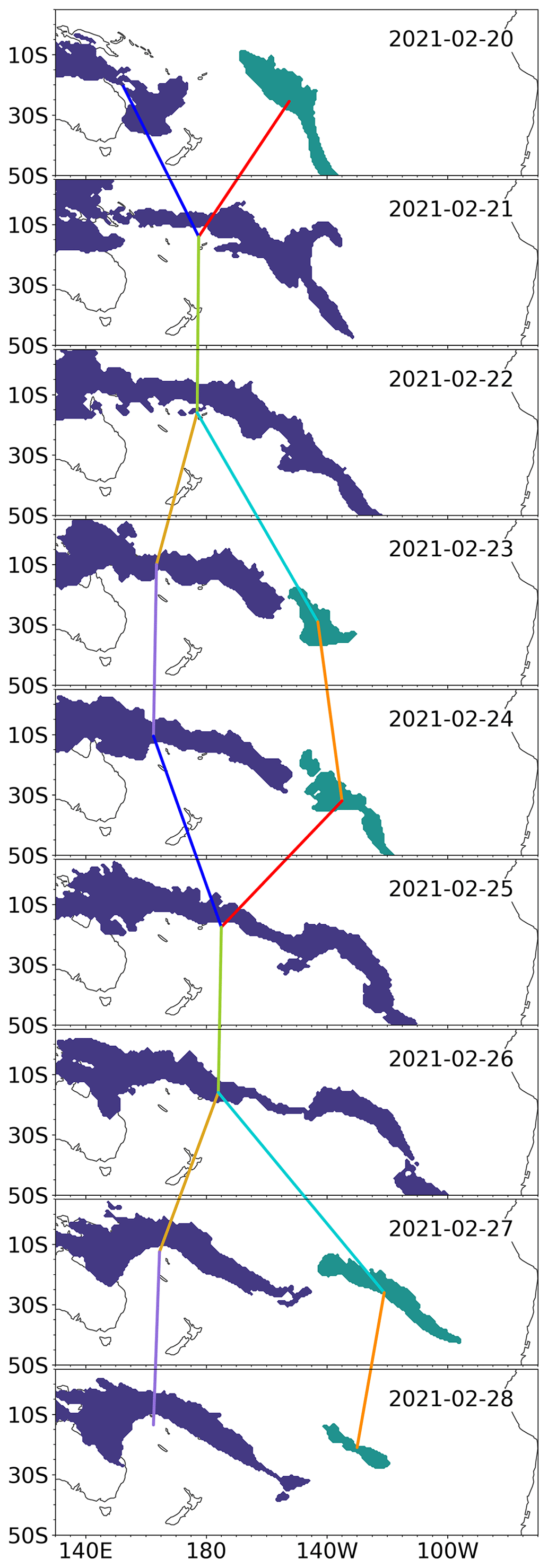
Figure 4 Example of splitting and merging of cloud bands, as well as their inheritance tracking from 20 to 28 February 2021 in the South Pacific Ocean. Lines connect the cloud bands' centroid locations. Colors are chosen to visualize merged (blue and red) versus split (gold and cyan) cloud bands.

Finally, a limitation associated with defining a specific domain for cloud band detection is that if a potential cloud band is on the boundary of the defined domain and its coverage within the domain is insufficient, the algorithm will discard such an object.

2.4 Inheritance tracking

To understand the life cycle of a cloud band and gain insights into the large-scale processes at play, we introduce an inheritance tracking method. This method focuses on establishing temporal connections between two consecutive cloud bands, distinctly different from traditional tracking methods used for tropical cyclones or MCSs. Our tracking method of cloud bands over time uses a simple area overlap method. Two-dimensional objects can be linked together across adjacent time frames based on the amount of overlap between them. Cloud bands with an area overlap between two consecutive time steps are considered the same, with the option for the user to define a specific overlap value. By default, any positive overlap area between two consecutive cloud bands is considered a single cloud band. We conducted tests with various overlap values ranging from 0 % to 100 % and found that any value between 0 % and 50 % overlap was suitable for our purposes, with 0 being too permissive. The overlap area is calculated in both time directions (i.e., from time t−1 to time t and from t to t+1), allowing us to determine the history and future of each cloud band and if a cloud band is either growing or shrinking in size. That is, the merging and splitting of cloud bands are treated explicitly. An example of splitting and merging of cloud bands is shown in Fig. 4. In this figure, cloud bands are detected from 20 to 28 February 2021 over the South Pacific. Initially, a cloud band in the western Pacific merges with another cloud band originating from the central Pacific between 20 and 21 February. Subsequently, the resulting cloud band persists for 2 d before splitting into two separate cloud bands on 23 and 24 February. These two bands then merge again on 24 and 25 February. It becomes apparent that the eastern segment of the cloud band slowly separates on 25 and 26 February, ultimately appearing as two distinct cloud bands on the 27 February. By 28 February, the easternmost cloud band begins to diminish in size, and the following day it is no longer detected (not shown in the figure).

Tracking methods in general provide information about the lifetime of the tracked features (Bengston et al., 1995; Camargo and Zebiak, 2002; Sugi et al., 2002; Chauvin et al., 2006). In this study, tracking tropical–extratropical cloud bands means knowing their inheritance from one time step to another. The tracking here does not provide information about the lifetime of a specific cloud band, and it does not indicate how long a specific cloud band lasts. Furthermore, as shown in Fig. 4, it is difficult to talk about the lifetime of a tropical–extratropical cloud band, especially if it is deeply rooted in the tropics, e.g., the quasi-permanent cloudiness over the SPCZ (Streten, 1973; Vincent, 1994; Brown et al., 2020). Focusing on the lifetime of a specific cloud band could lead to the workflow identifying long periods wherein a single cloud band persisted, despite the likelihood that the initial identified cloud band may have split into two different ones and merged with another one, for example with a trough intruding from the midlatitudes (Kiladis et al., 1989). However, in other basins where cloud bands are often associated with transient weather systems (see Fig. 5) the lifetime of such weather systems may be relevant.

2.5 Implementation and configuration

The method developed in this study is embedded in a Python package called cloudbandPy. Installation can be done using the Pip package management system (The Pip Development Team, 2021) or the Conda environment setup (Anaconda, Inc., 2016). Environment, requirement files, and installation instructions are provided here: https://github.com/romainpilon/cloudbandPy (last access: 13 March 2024). All user-defined parameters are stored in a YAML file (https://yaml.org/, last access: 13 March 2024) for easy access and modification. The configuration file specifies dates, study domains, data location, and which steps to run. As an example, loading 1 year of 0.5° horizontal resolution OLR data from ERA5, the detection of cloud bands and writing files that contain all detected cloud bands takes less than 1 min using an AMD EPYC processor.

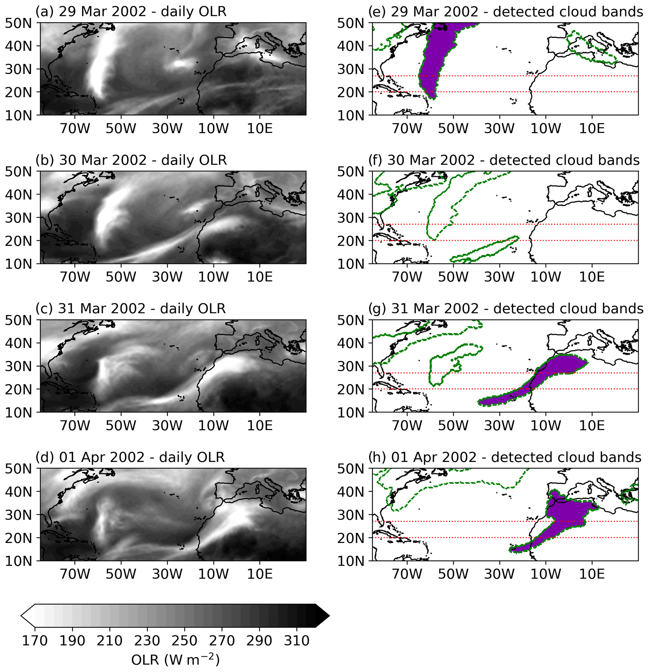
Figure 5 Snapshots of (a–d) OLR as well as of (e–h) associated detected cloud bands (shading) and of identified features, i.e., potential cloud bands (dashed contours) over the North Atlantic basin from 29 March to 1 April 2002. The horizontal lines represent the latitudinal lines that cloud bands must cross to be defined as a tropical–extratropical cloud band.

3 Application to ERA5 reanalysis data

We envisage that the algorithm presented here will be used for assessing tropical–extratropical connections in different datasets including global climate simulations, and we now present a few examples of such applications. All examples briefly discussed in this section are included in the public repository linked to in the “Code and data availability” statement.

3.1 Case study

Among the cloud bands in the literature that satisfy the criteria chosen here, we select a well-documented cloud band resulting from tropical–extratropical interaction, which was extensively investigated by Knippertz (2005) (hereafter referred to as KP05). This cloud band (“tropical plume”) is described as an elongated band of upper- and mid-level cloud formation stretching from the central tropical Atlantic Ocean to the northern African continent accompanied by a subtropical jet streak from 29 March to 1 April 2002. The evolution of this specific cloud band with a latitudinal tilt is shown with daily average of OLR in Fig. 5a–d and in satellite infrared imagery (Fig. 2 from Knippertz, 2005).

Although this basin falls outside of our primary areas of interest, which focus on basins with a tropical–extratropical convergence zone, this cloud band serves as an excellent test bed and provides insights into the behavior of our algorithm. For this particular event, we perform the detection process in the entire Northern Hemisphere. In Fig. 5e–h, both cloud bands and the identified features (obtained from the step illustrated in Fig. 1e) are displayed. On 29 March 2005, our algorithm detects a cloud band in the western Atlantic with a strong inclination, spanning from the Caribbean to the western coasts of Canada. The following day, this cloud band shifts poleward and is no longer classified and labeled as a tropical–extratropical cloud band by our algorithm (its southern tip is at 21° N on 30 March and at 23° N on 31 March); the northern section of this unlabeled cloud band shifts eastward along with the midlatitude circulation. The midlatitude segment of the unlabeled cloud band dissipates by 31 March, and on 1 April, no further features are detected.

In KP05, the cloud band that reaches western Africa becomes visually apparent on 30 March 2005. Our detection identifies a feature initially in the central tropical Atlantic Ocean, but it is disregarded due to insufficient spatial extent (based on the latitudinal extent criterion). However, the cloud band itself is successfully detected on 31 March.

3.2 Spatial distribution of cloud bands

Long-term global detection allows for an illustration of the spatial distribution of tropical–extratropical cloud bands. The spatial distribution of cloud bands is illustrated in Fig. 6, showing a climatology of the number of cloud band days per year per grid point from 1959 to 2021. Cloud bands are detected only between 10 and 50° N and between 10 and 50° S to avoid misidentifying tropical–extratropical cloud bands as mentioned in Sect. 2.3. The figure clearly illustrates the presence of the four tropical convergence zones, as indicated by the highest number of cloud band days per year. The SPCZ and the SICZ exhibit maxima of 49 and 28 cloud band days per year, respectively. Cloud bands from the BFZ merge here, with cold cloud cover from the Tibetan plateau and from the South Asian monsoon, which are also labeled as cloud bands. In the northeastern Pacific region, from Hawaii to the south of California, notable occurrences of cloud bands, commonly referred to as atmospheric rivers, are observed (on average from 1 to 2 weeks per year). It is worth noting that long cloud spirals trailing away from the centers of tropical cyclones may also be identified as cloud bands. Additionally, in the eastern tropical Atlantic Ocean and the western Sahara, there are instances of cloud bands, including the one discussed in KP05 and depicted in the previous section. The North Atlantic basin does not exhibit a convergence zone; hence, it contains few cloud bands. The northern Caribbean experiences approximately 14 cloud band days per year, potentially influenced by tropical cyclones, compared to 21 cloud band days in the northeastern Pacific region, which is also influenced by tropical cyclones and by atmospheric rivers.

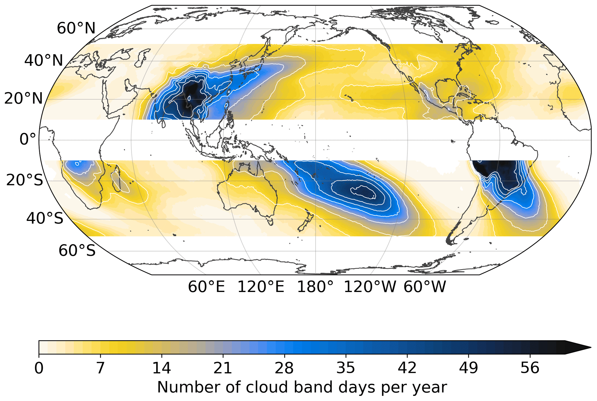
Figure 6 Number of cloud band days per year averaged from 1959 to 2021. Contour interval: 7 cloud band days per year.

To mitigate the issue of false detections (i.e., non-diagonal tropical–extratropical cloud bands) in spatial distributions, it is preferable to conduct the detection process separately for each basin in order to account for features that are specific to the respective geographical region. This can be achieved by considering the four defined domains in the study. To illustrate this approach, Fig. 7 depicts the average number of cloud band days per year, computed from 1959 to 2021, overlaid on the Global Precipitation Climatology Project (GPCP) data (Huffman et al., 2020). The GPCP data combine satellite and gauge measurements of precipitation.

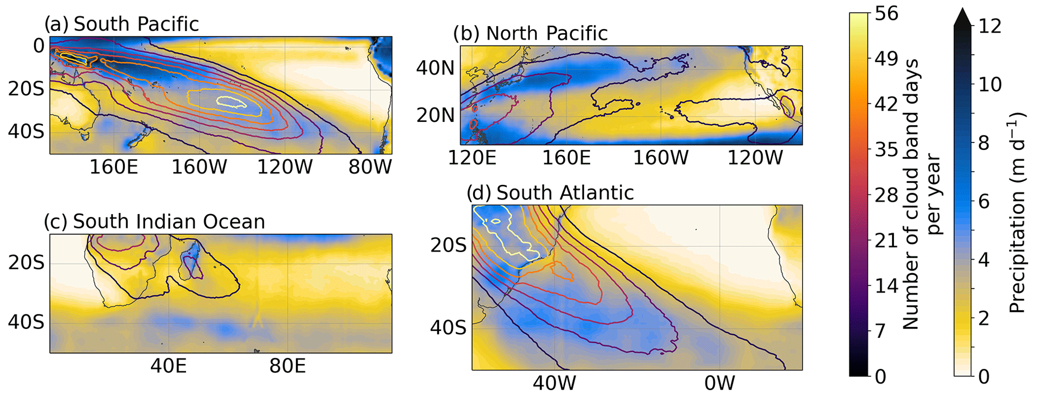
Figure 7 Mean precipitation rate in mm d⁻¹ from the GPCP precipitation data from 1983 to 2019 (shading), overlaid by the number of cloud bands per year averaged over the same period (contour interval: 7 cloud band days per year). Contours correspond to contours in Fig. 6 but the detection is performed separately for the four domains.

The SPCZ (Fig. 7a) exhibits a maximum occurrence of cloud bands in the central Pacific, situated at the southeasternmost mean position of the SPCZ (Vincent et al., 2011). This region, situated south of French Polynesia, experiences approximately 2 months of cloud band days per year. This maximum occurrence of cloud bands is positioned between two precipitation maxima in the central Pacific region: one of these maxima is associated with midlatitude dynamics, while the other originates from the SPCZ itself.

In the North Pacific region (Fig. 7b), the occurrence of cloud bands displays a peak (35 d of cloud bands per year) between two areas characterized by heavy precipitation: the BFZ and the Maritime Continent. Additionally, in the northeastern part of the North American continent, the detection of cloud bands suggests a potential association with cloud cover resulting from midlatitude Rossby wave breaking, which instigates convection and can lead to heavy precipitation (Kiladis and Weickmann, 1992; Knippertz, 2007; de Vries, 2021).

In the southern part of the African continent and the southwestern Indian Ocean (Fig. 7c), the distribution of cloud bands follows a similar pattern to that of the SICZ, which is influenced by the circulation around the Angola Low, the northeastern monsoon region, and the southern Indian Ocean high-pressure system that extends over the continent (Cook, 2000; Ninomiya, 2008). This pattern of cloud bands in the region was previously observed by Hart et al. (2012) using OLR data with coarser resolution (2.5°). Among the four convergence zones, the SICZ displays relatively lower activity in terms of cloud band days per year, with a maximum of 21 d cloud band days per year. Additionally, this convergence zone demonstrates lower surface precipitation compared to other convergence zones, mainly owing to the predominance of rainfall during the summer months across most inland regions and during the winter months along the Western Cape coastal areas (Harrison, 1984). Moreover, precipitation is modulated by the Madden–Julian oscillation (Pohl et al., 2007).

Finally, in the case of the SACZ (Fig. 7d), the region extending from southern Amazonia to the southeast coastal regions of Brazil exhibits the highest annual occurrence of cloud bands, with 56 cloud band days per year. Over the South Atlantic Ocean, lower cloud band occurrences ranging from 21 to 35 d per year are observed. Our findings align with the spatial distribution of OLR in the presence of an intense and continental SACZ, as defined by Carvalho et al. (2004). Furthermore, the dominant role of deep convection in the southern Amazon Basin and the southeastward extension of low OLR values into the Atlantic have been previously highlighted (Liebmann et al., 1999; Carvalho et al., 2002). Precipitation from the GPCP reveals two distinct regions of strong precipitation. One is located over the southern Amazon Basin, while the other extends over the South Atlantic Ocean, encompassing parts of southern Brazil and Uruguay. The oceanic region is influenced by midlatitude dynamics and Rossby wave breaking (Liebmann et al., 1999; Zilli and Hart, 2021).

3.3 Climatology and temporal evolution

The use of automated detection techniques facilitates the study of the variability associated with cloud bands. In this regard, Fig. 8 presents the time series of the annual frequency of cloud bands (Fig. 8a) and of the mean area covered by cloud bands (Fig. 8b) across the four aforementioned domains.

The South Pacific domain stands out with the highest annual occurrence of cloud bands, highlighting the strong convective activity of the SPCZ (Vincent et al., 2011; Dowdy et al., 2012) deeply entrenched in the tropical region and including the Maritime Continent, compared to the other three convergence zones. The intrusion of fronts from the midlatitudes into the South Pacific further increases the mean annual occurrence of cloud bands, as multiple cloud bands can be present in a single day (Fig. 4). The North Pacific domain sees between 100 and 200 cloud band days per year. In this domain, our algorithm captures cloud bands from the BFZ but also cloud bands associated with eastward-propagating disturbances (Huaman et al., 2020) and atmospheric rivers (Dettinger et al., 2011). Over the South Atlantic domain, the occurrence of cloud bands ranges from 60 to 150. Some of the SACZ and its associated cloudiness are located outside, northwest of the domain we define, which is discussed in Sect. 2.3. Hence, the algorithm cannot detect some of the land-based cloud systems than might account for some of the cloud band day occurrence. In contrast, the southern Indian Ocean (yellow line in Fig. 8) demonstrates the lowest occurrence of cloud bands. The cool and highly variable sea surface temperatures over the SICZ lead to less intense convective activity and cloud band formation (Shannon et al., 1990) compared to other convergence zones. Moreover, the SICZ is a land-based convergence zone whose intensity is partially influenced by surface conditions over southern Africa, with its intensity partially determined by surface conditions over southern Africa. This characteristic results in a stronger annual cycle and intermittent behavior compared to the other convergence zones (Cook, 2000).

The magnitude of the time series, depicting the number of cloud bands per year, is consistent with the spatial patterns of cloud band occurrence displayed in Fig. 7 and closely follows the evolution of the mean area covered by the cloud bands.

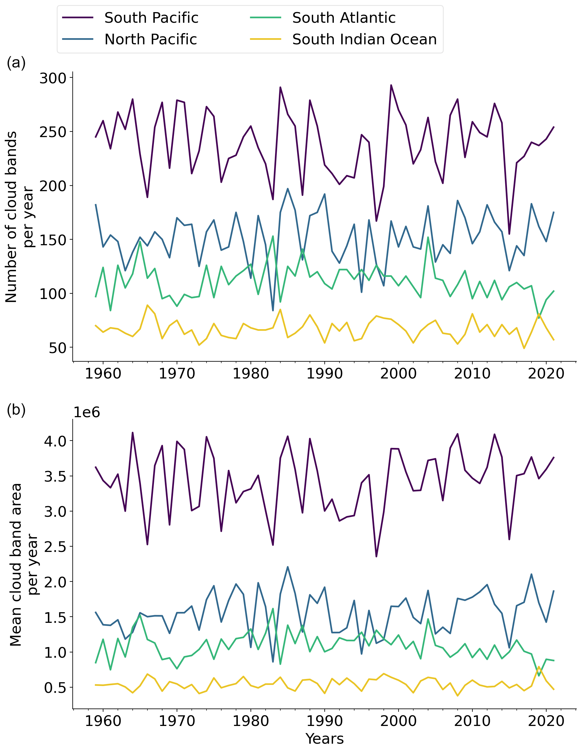
Figure 8 Time series of (a) the number of cloud bands per year for each domain defined in Fig. 2 and (b) of the mean cloud band area per year (expressed in km²).

A similar picture emerges in the seasonal cycle as shown in Fig. 9, which represents the annual cycle of cloud bands and of their mean area per basin, averaged from 1959 to 2021. The seasonal cycles of the respective domains follow the seasonal cycle of convective activity and precipitation. Moreover, the seasonal variations in the mean area covered by cloud bands closely mirror the fluctuations in the number of cloud bands. For example, in the South Pacific, cloud bands are the dominantly present during austral summer, in agreement with findings from Vincent (1994) and Matthews (2012), and the cloud bands show a strong seasonal cycle with around 3 times more cloud band days per month during austral summer than during austral winter. The variability between seasons in the North Pacific domain is low, with only a twofold increase in cloud band days during the summer season. In the South Atlantic, the magnitude of the annual cycle of cloud bands over the SACZ is similar to the findings of Zilli and Hart (2021). Moreover, because this convergence zone is more strongly rooted in the subtropics and over land, convection and associated cloudiness are more strongly affected by seasonality (Paegle et al., 2000; Jones and Carvalho, 2002; Carvalho et al., 2004). The seasonal cycle of cloud band days over the South Atlantic ranges from 2 to 20 cloud bands per month during the winter/dry season and the summer/wet season, respectively. The southern Indian Ocean exhibits the fewest cloud bands per month among all the domains. There is an extended period of no or very few cloud bands from June to September. We find more cloud bands per month compared to Hart et al. (2013), who find that the seasonal cycle from 1979 to 1999 ranges from 0 to 5 cloud bands per month and who used a domain smaller than ours.

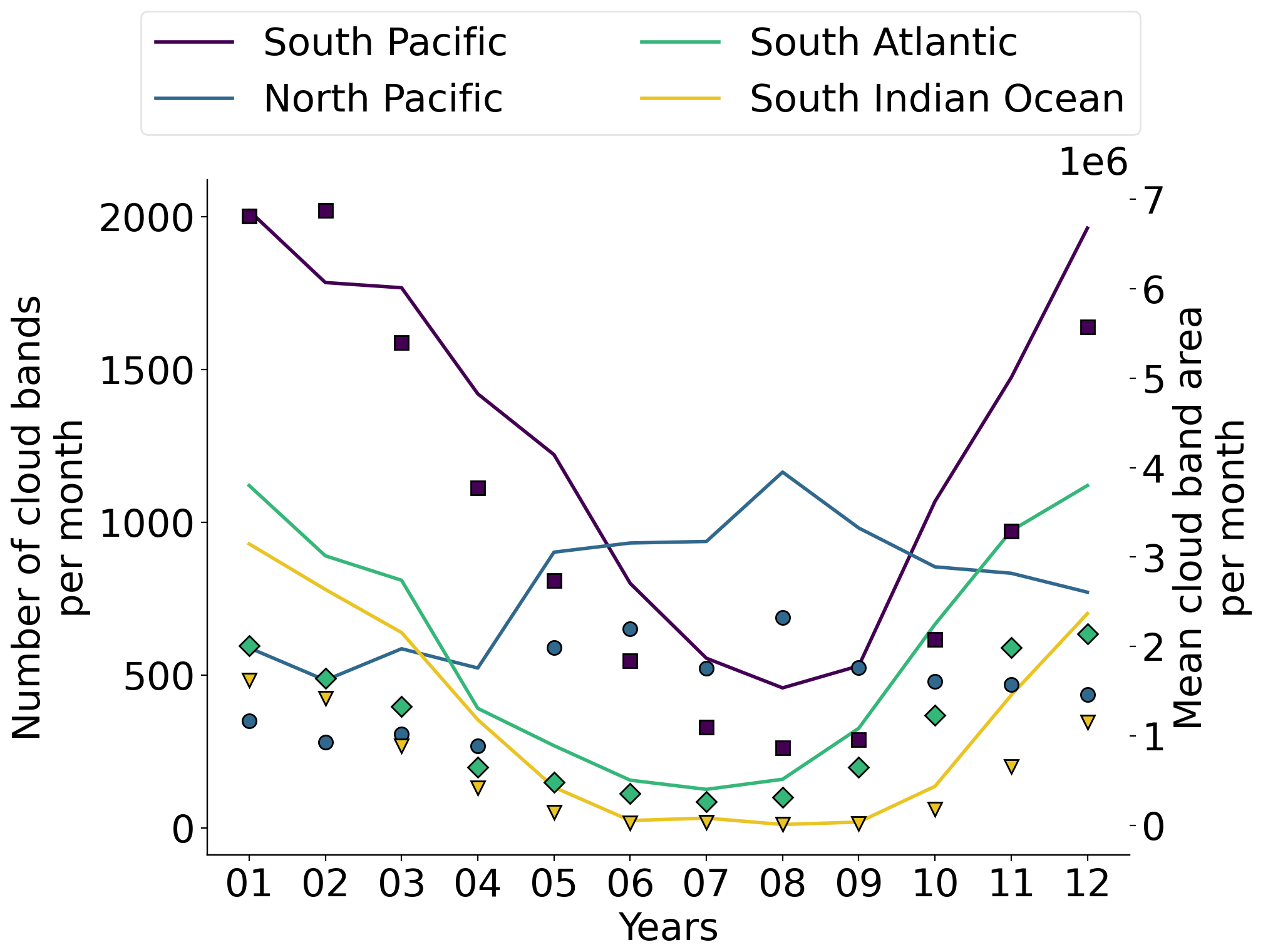
Figure 9 Annual cycle of the number of cloud bands per month (lines) for each domain defined in Fig. 2, overlaid by the annual cycle of mean cloud band area (markers: squares – South Pacific, circles – North Pacific, diamonds – South Atlantic, triangles – southern Indian Ocean). Marker colors correspond to line colors.

4 Discussion and conclusion

In this study we develop a Python-based tool for efficiently detecting atmospheric tropical–extratropical cloud bands, aiming to better understand their spatiotemporal distribution and associated atmospheric processes. This tool will facilitate the connection of large-scale processes bridging the tropics and extratropics, using cloud bands as a proxy for further studies.

This novel tool combines thresholding and labeling methods and allows for explicit merging and splitting of cloud bands using conventional area overlapping. We specifically focus on using OLR data. The identification algorithm is developed to handle a variety of weather and climate datasets, such as high-resolution reanalyses or model simulations. In addition, a flexible interface has been designed so that users can apply their own criteria for the identification of cloud bands or use other variables for detection such as brightness temperature. All user-definable parameters are specified in a configuration file that contains detailed explanations for ease of use. Additional features of interest can be implemented without much coding due to the modular framework design. The package can be run on small or high-performance computers and can rapidly create cloud band datasets. The algorithm code is publicly available, facilitating further refinement of the method. Various visualization and statistical analysis examples are provided in the package. We demonstrate the capability of this algorithm to detect diagonal cloud bands in different basins chosen based on the location of the major convergence zones.

In the context of our methodology, it is necessary to acknowledge certain limitations. Firstly, it is important to note that OLR is a derived variable that depends on both temperature and emissivity, unlike brightness temperature, for example. This sensitivity may lead to misidentification of cloud bands. Secondly, context and application play a crucial role in selecting threshold values, as different values may be suitable depending on the specific use case. For example, previous studies by Hart et al. (2012) and Hart et al. (2018) primarily examined the midlatitude section of tropical–extratropical cloud bands, which exhibit less convective activity. These studies adopted a higher OLR threshold, encompassing a wider range of cloud types. In our study, we specifically focused on identifying cloud bands characterized by convection and set an OLR threshold value according to the OLR distribution associated with deep convection. To further optimize our methodology, it would be preferable to use a relaxed OLR value instead of a morphological expansion. This adjustment would ensure a more accurate consideration of the real OLR values surrounding identified cloud systems before initiating the labeling step. Finally, our software is designed solely for the detection of tropical–extratropical cloud bands. While this focus aligns with our primary objective, it is conditioned by the specific criteria we use to identify and classify these cloud bands. These criteria, while effective for our intended area, may not be universally applicable to cloud detection in various atmospheric conditions and regions.

Alternative thresholding methods were tested, such as global thresholding methods (see Appendix A), which automatically select optimal threshold values based on data. While useful for certain applications, if used globally, these techniques may lead to mislabeling features as cloud bands, particularly in situations with significant temporal and spatial variability in OLR values, encompassing regions such as the Tibetan plateau, South Asian monsoon, and BFZ. Hence, careful interpretation and domain refinement are important, which necessitates selecting appropriate domain limits. Domains are provided in the code. Using the algorithm in specific domains can therefore improve the accuracy of the detection and allows for a better characterization of cloud bands over convergence zones. Further regional refinements will still be required in order to limit the detection to cloud bands.

Another approach is to use machine learning techniques (Cilli et al., 2020; Beucler et al., 2021; Prabhat et al., 2021), which can automatically select the best threshold values based on the data and the studied phenomena (see Appendix A). These models can evaluate multiple features and their interactions to determine the optimal threshold values for each feature, without requiring manual tuning or manual labeling.

Further developments could include combining cloud features with precipitation features similarly to techniques for tracking MCSs (e.g., Yuan and Houze, 2010; Fiolleau and Roca, 2013; Feng et al., 2023). This approach allows for unrestricted global tracking and improves the detection of tropical–extratropical cloud bands, while separating cloud cover from non-cloud-band regions. In addition, future enhancements may focus on automatic detection of cloud bands regardless of the mapping convention used in the input data.

The demonstrated method can then be used for further investigations of cloud band climatology as well as for studying connections with synoptic processes.

Appendix A: Use of global thresholding method

In image processing applications, thresholding, also known as image segmentation, is a technique used to separate objects or regions of interest from an image based on their pixel intensity values. It involves selecting a fixed threshold value that acts as a cutoff point. The threshold value is a pixel intensity value used to separate the pixels into two groups: those with intensities above the threshold are assigned to the background, and those with intensities below the threshold are assigned to the foreground. In this study, the foreground corresponds to clouds, the background corresponds to clear sky, and the pixel intensity corresponds to the OLR threshold value.

Other and more objective techniques exist, such as global thresholding methods. Contrary to simple thresholding techniques with a fixed threshold, global thresholding methods automatically determine the threshold value by selecting a single value that minimizes the variance between the foreground and background pixels based on the histogram of the image. Global thresholding methods hold promise for greater objectivity compared to thresholds determined subjectively by humans, as they do not rely on specific phenomena observed in a limited number of cases.

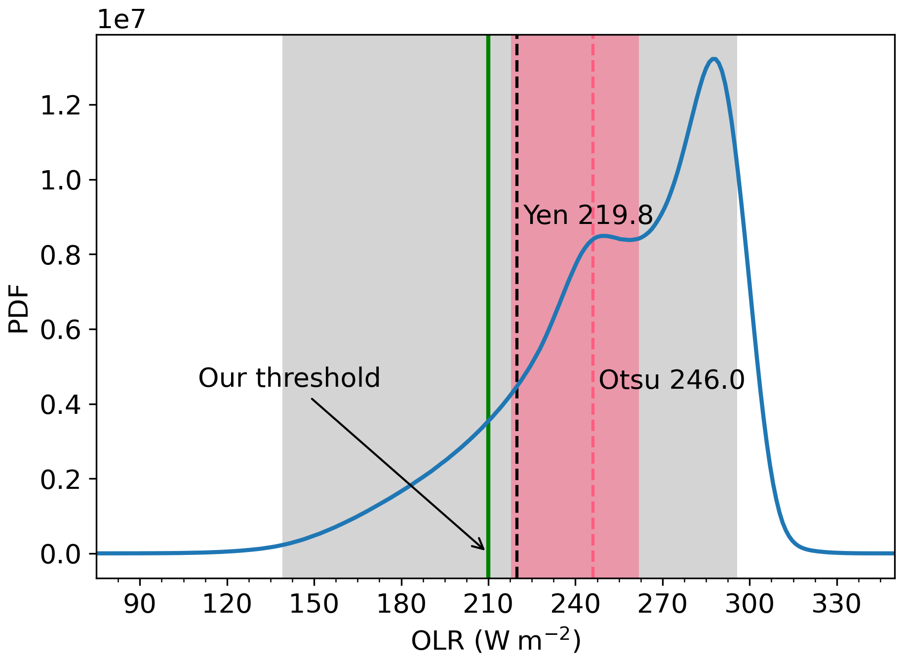
Figure A1 Distribution of OLR values for each grid point of the South Pacific domain covering 130–290° E and 5° N–50° S (see Fig. 2). The vertical green line represents the threshold value used in our study. The vertical dashed lines represent the median threshold values obtained from applying the Yen and Otsu automated thresholding methods (see explanations in the text). The gray and pink shaded areas indicate the range of values found for each day of the period, from the minimum to the maximum, for the Yen and Otsu thresholding methods, respectively.

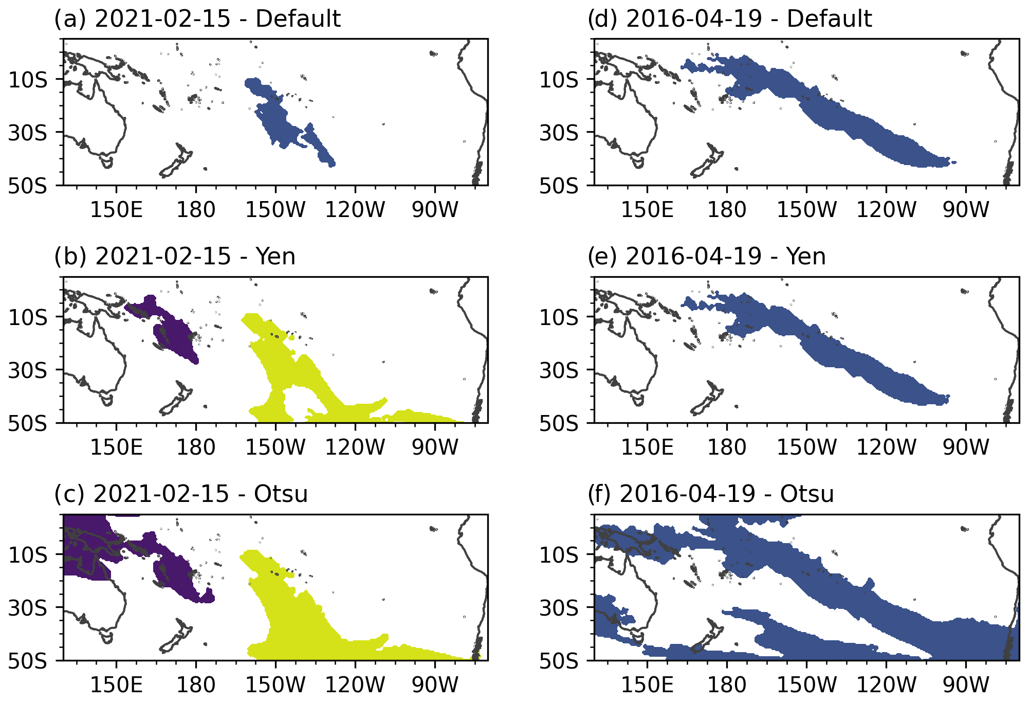
Figure A2 Comparison of cloud band detections using various thresholding techniques on 15 February 2021 and 19 April 2016. The images in panels (a) and (d) were processed using the threshold value from this study (i.e., 210 W m⁻²), while panels (b) and (e) utilized the Yen thresholding technique and (c) and (f) utilized the Otsu thresholding technique.

However, these methods have limitations when the object (the cloud band) of interest in the foreground is not well separated from the background or when values (in this case OLR) are irregular across the image. Moreover, this technique and more advanced ones, such as adaptive thresholding or edge-based segmentation, have been developed mainly for contrasting images with edges, such as for optical character recognition to convert an image of text into text format. Such methods were developed mainly to make details visible throughout data and may not be applicable to the same degree when studying physical objects without clear boundaries.

We tested two popular approaches: (1) the Otsu method (Otsu, 1979), which is particularly useful when there is a bimodal distribution of pixel intensities in the image, such as the OLR distribution shown in Fig. A1, and (2) the Yen method (Yen et al., 1995), which finds an optimal threshold by minimizing the difference between the probability distributions of pixel intensities between the foreground and background regions at each time step. The Yen method is particularly relevant for identifying features in scattered data.

Figure A1 shows the probability distribution of OLR over the South Pacific domain using all grid points and all days from 1960 to 2021. The distribution is bimodal with two peaks at 250 and 295 W m⁻². The Yen and Otsu methods yield threshold values of approximately 220 and 246 W m⁻² indicated by the vertical lines, respectively. The Otsu median threshold value proves to be excessively high for detecting tropical–extratropical cloud bands composed of convective systems (Massie et al., 2002), hindering the detection of cloud bands composed of warmer clouds with higher OLR values. Consequently, the detected features in Fig. A2c and f do not solely represent tropical–extratropical cloud bands.

On the other hand, the Yen median value of around 210 W m⁻² aligns more closely with our chosen threshold and has a higher likelihood of accurately detecting cloud bands (Fig. A2e). However, in some cases, the value calculated with the Yen method is still too high to effectively detect tropical–extratropical cloud bands, leading our algorithm to merge different features. For example, in Fig. A2b, the central Pacific cloud band is merged with two midlatitude troughs. During the development stage of our algorithm, we opted for a more restrictive approach and then expanded the detected feature using morphological dilation, as described in Sect. 2.2.

Moreover, the shaded areas in Fig. A2 represent the range of threshold values calculated for each day of the period. The wide range of values indicates a significant daily variability. It is noteworthy that on certain days with no cloud bands, the global thresholding method may still identify a feature to extract from the image, typically characterized by the lowest contiguous OLR values at each time, potentially mislabeling this feature as a cloud band (Fig. A2f).

Appendix B: Sensitivity test on OLR threshold

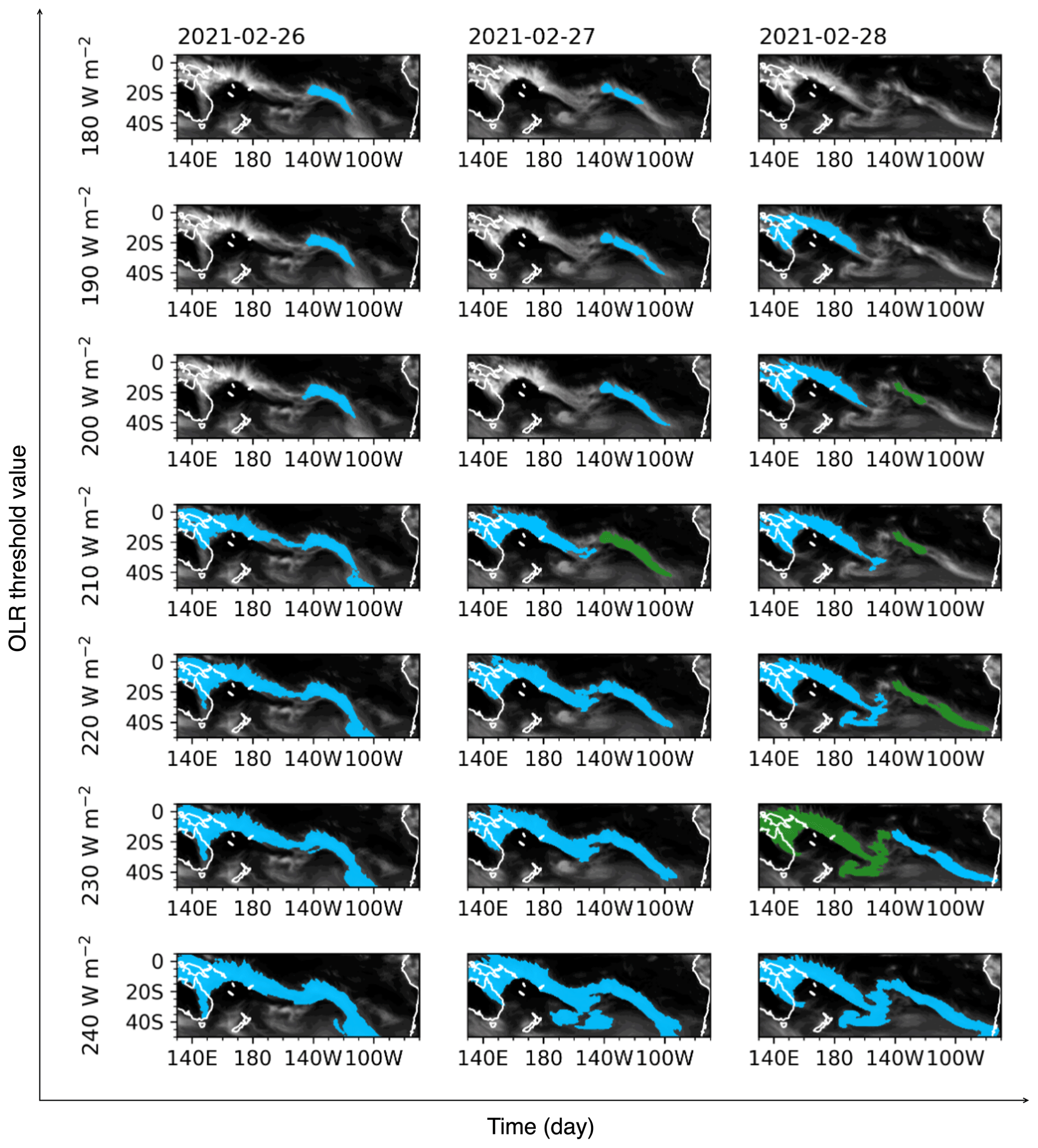
Figure B1 Sensitivity test case illustrating the detection of cloud bands in relation to the OLR threshold, ranging from 180 to 240 W m⁻² with an interval of 10 W m⁻², from 26 to 28 February 2021 in the South Pacific.

We conducted a sensitivity test on the OLR threshold to check the performance of the algorithm in detecting the cloud bands shown in Fig. 4 and their evolution. We used values between 180 and 240 W m⁻² with an interval of 10 W m⁻². Figure B1 illustrates that using an excessively high threshold for OLR at 240 W m⁻² results in the identification of a single cloud band instead of the expected two. In addition, the algorithm incorrectly detects extratropical clouds that do not belong to a specific cloud band but are instead mistakenly identified as part of the cloud band. The detection does not allow cloud band splitting and merging in this example. Conversely, when using the lowest OLR threshold of 180 W m⁻², it is evident that the algorithm has difficulty identifying any cloud bands, especially in tropical regions. In particular, the detection of cloud systems in the tropics during the entire period (especially clouds from the SPCZ) only begins at an OLR threshold of 210 W m⁻². However, the user may find that the SPCZ is identified too often as a cloud band and would then choose a threshold around 200 W m⁻², as in Rosa et al. (2020).