Deep learning applied to CO₂ power plant emissions quantification using simulated satellite images

The quantification of emissions of greenhouse gases and air pollutants through the inversion of plumes in satellite images remains a complex problem that current methods can only assess with significant uncertainties. The anticipated launch of the CO₂M (Copernicus Anthropogenic Carbon Dioxide Monitoring) satellite constellation in 2026 is expected to provide high-resolution images of CO₂ (carbon dioxide) column-averaged mole fractions (XCO₂), opening up new possibilities. However, the inversion of future CO₂ plumes from CO₂M will encounter various obstacles. A challenge is the low CO₂ plume signal-to-noise ratio due to the variability in the background and instrumental errors in satellite measurements. Moreover, uncertainties in the transport and dispersion processes further complicate the inversion task.

To address these challenges, deep learning techniques, such as neural networks, offer promising solutions for retrieving emissions from plumes in XCO₂ images. Deep learning models can be trained to identify emissions from plume dynamics simulated using a transport model. It then becomes possible to extract relevant information from new plumes and predict their emissions.

In this paper, we develop a strategy employing convolutional neural networks (CNNs) to estimate the emission fluxes from a plume in a pseudo-XCO₂ image. Our dataset used to train and test such methods includes pseudo-images based on simulations of hourly XCO₂, NO₂ (nitrogen dioxide), and wind fields near various power plants in eastern Germany, tracing plumes from anthropogenic and biogenic sources. CNN models are trained to predict emissions from three power plants that exhibit diverse characteristics. The power plants used to assess the deep learning model's performance are not used to train the model. We find that the CNN model outperforms state-of-the-art plume inversion approaches, achieving highly accurate results with an absolute error about half of that of the cross-sectional flux method and an absolute relative error of ∼ 20 % when only the XCO₂ and wind fields are used as inputs. Furthermore, we show that our estimations are only slightly affected by the absence of NO₂ fields or a detection mechanism as additional information. Finally, interpretability techniques applied to our models confirm that the CNN automatically learns to identify the XCO₂ plume and to assess emissions from the plume concentrations. These promising results suggest a high potential of CNNs in estimating local CO₂ emissions from satellite images.

1 Introduction

The burning of fossil fuels, such as coal and oil, in power plants (PPs), is a primary source of anthropogenic CO₂ (carbon dioxide) emissions. Approximately 50 % of worldwide fossil fuel CO₂ emissions originate from large facilities, which encompass PPs (IEA, 2019; Nassar et al., 2022). As a result, maintaining regular monitoring of these emissions and possessing the capacity to control their reporting are crucial.

Observations from satellites like OCO-2 provide valuable data that can be utilised to estimate CO₂ emissions (Nassar et al., 2017; Reuter et al., 2019; Chevallier et al., 2019; Wu et al., 2020; Zheng et al., 2020; Nassar et al., 2022; Chevallier et al., 2022). Specifically, satellite observations of CO₂ plumes, such as the plume transects obtained from OCO-2 and OCO-3 satellites, offer a direct means of quantifying their source and complement other estimations (Cusworth et al., 2021). The upcoming launch of the Copernicus Anthropogenic Carbon Dioxide Monitoring (CO₂M) satellites in 2026 is anticipated to capture high-resolution images of CO₂ column-averaged mole fractions (XCO₂), aiming to have a much larger swath and more accurate CO₂ estimations and further advancing our capabilities in this area. Leveraging these images, however, will present significant challenges (Wang et al., 2020).

CO₂ plumes are notoriously difficult to invert due to various factors, including (1) image integrity issues caused by cloud cover or satellite overpasses, which result in missing data in the images used for analysis. Additionally, the estimation of the emissions associated with a plume is further complicated by (2) the low signal-to-noise ratio (SNR) of the measurements. The noise component encompasses variations in the background as well as errors in the satellite measurements. The SNR problem stands as the main hurdle in the detection of the plume, a crucial step for inversion. Recent research conducted by Dumont Le Brazidec et al. (2023a) has illustrated the remarkable ability of convolutional neural networks (CNNs) to effectively overcome this obstacle. Lastly, another challenge stems from (3) the uncertainties in the transport and dispersion processes, specifically, when it comes to estimating the effective wind driving the plume and determining its shape (Kuhlmann et al., 2019).

This paper addresses the second and third problems (except for the errors in the satellite measurements) by employing deep learning techniques to perform inverse modelling of CO₂ plumes. In particular, we focus on developing techniques for inverting CO₂ plumes from PPs of different emission levels.

To assert the effectiveness of the method, the predictions of the deep learning model are compared against state-of-the-art techniques. Plume inversion methods include approaches that use an atmospheric transport model to simulate the plume and compare it to observations (e.g. Pillai et al., 2016; Broquet et al., 2018). They also include techniques that quantify emissions from a hotspot based on plume detection in satellite observations (Koene et al., 2021). These methods can be based on time-averaged plumes, such as the divergence method (Beirle et al., 2019; Hakkarainen et al., 2022), or on instantaneous images. Varon et al. (2018) compared several of these approaches, namely the Gaussian plume inversion, the integrated mass enhancement, and the cross-sectional flux method. In the CoCO2 project, several of these methods were compared using synthetic CO₂M CO₂ and NO₂ (nitrogen dioxide) observations (Hakkarainen et al., 2023). Here, we use the cross-sectional flux (CSF) method for comparison, which showed similar accuracy to other well-performing methods such as Gaussian plume inversion and the light cross-sectional flux (LCSF) method. Finally, it should be noted that the CoCO2 project identified several potential improvements of these methods that may yield superior performance in the future (Hakkarainen et al., 2023; Santaren et al., 2024).

In this paper, the proposed plume inversion approach is based on convolutional neural networks. This research builds on earlier work in the field of remote sensing image analysis leveraging machine learning techniques (Lary et al., 2016; Finch et al., 2022; Jongaramrungruang et al., 2021; Joyce et al., 2023; Kumar et al., 2023). Here, plume inversion involves the analysis of an image to extract a scalar or a vector of emissions at different time steps. Therefore, this task can be framed as an image regression problem, where relying on CNNs can offer significant advantages (Chollet, 2017). CNNs can be trained on a comprehensive dataset, where all input variables (images) and associated output variables (like emissions) are known. Once trained, these CNNs can effectively process and draw conclusions from unseen observational imagery. CNNs employ convolutional layers to extract essential features from images. Each filter is automatically trained to detect specific patterns, such as edges, corners, or other shapes within the image. By stacking multiple convolutional layers, CNNs become capable of learning intricate patterns, enabling them to capture increasingly complex features. The ability of CNNs to capture and learn spatial features in images makes them a popular choice for various image-related tasks, including image recognition, classification, and regression. Given the nature of our plume inversion task, they are particularly well-suited due to their ability to identify spatial features in images, such as plume shapes or intensity, that correspond to specific emissions. This feature extraction approach effectively harnesses the knowledge embedded in transport models, enabling this automatic capture of plumes dynamics. This ability to capture such features has already been demonstrated by Finch et al. (2022) or Dumont Le Brazidec et al. (2023a), who studied the segmentation of plumes in CO₂ images.

To train and test the CNN models, this paper relies on a synthetic dataset as CO₂M data will not be available until 2026. This dataset has been designed to possess similar key features to the forthcoming CO₂M satellite, such as resolution and the availability of NO₂ data. However, the influence of clouds or systematic error patterns is not considered in the analysis.

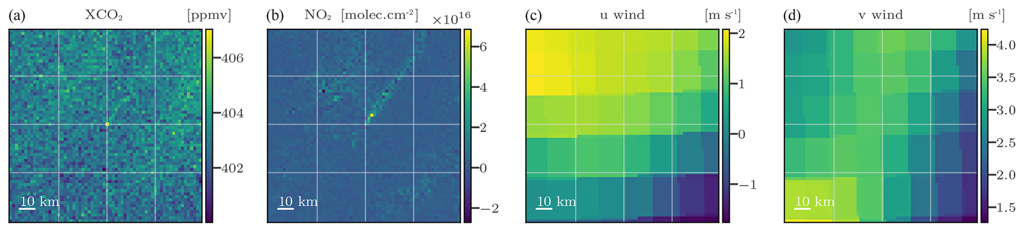
Figure 1 Examples of inputs used by the CNN model. Panels (a)–(d) represent the XCO₂ images, NO₂ images, and vertically averaged u and v winds, respectively.

Before introducing the inversion methodology and results, we briefly describe the physical fields used to train and evaluate the CNNs. This includes the presentation of the simulated satellite fields in Sect. 2 and of the model used to produce segmentation masks of the plumes used as inputs of the inversion model in Sect. 3. The inversion methodology using CNN is described in Sect. 4, specifying the problem statement, the model, the training process, and the alternative method employed for comparison. The subsequent Sect. 5 delves into the application of the model to three specific PPs. In particular, Sect. 5.3 places special emphasis on the interpretability of the trained CNNs. Discussions on the limitations and future directions of this study can be found in Sect. 6, while the conclusions are outlined in Sect. 7.

2 Dataset of XCO₂, winds, and NO₂ images

XCO₂ and NO₂ images are taken from the concentration fields simulated for the SMARTCARB project (Brunner et al., 2019). Using the COSMO-GHG model, the SMARTCARB simulations were performed in a region centred on Berlin and covering several nearby coal-fired PPs. These simulations were used to produce synthetic observations of CO₂M and to evaluate various plume detection and inversion approaches (Kuhlmann et al., 2019, 2020a, 2021; Hakkarainen et al., 2021, 2023). The data are hourly and cover an entire year. Their spatial resolution is 0.01°, and 60 vertical layers ranging spanning from an altitude of 0 to 24 km are used. More information can be found in Dumont Le Brazidec et al. (2023a), who presented more extensively a dataset very similar to the one used in this study.

Images used to train and evaluate the CNN inversion models consist of 64 × 64 pixels, with each pixel covering an area of 2 km × 2 km. Each image is extracted from the SMARTCARB COSMO-GHG simulated fields so that one hotspot is located in the centre. In addition, the selected size guarantees the inclusion of the majority of the central hotspot plume within the image. The mapping from the original SMARTCARB fields' resolution to the 2 km resolution is performed by cubic spline interpolation (Virtanen et al., 2020). The 2 km resolution was chosen to be consistent with the resolution expected for CO₂M observations.

It is necessary to take into account the expected noise associated with the satellite instruments. For this, Gaussian random noise of standard deviation 0.7 ppm, characteristic of the CO₂M (Meijer, 2020), is added to the XCO₂ images.

In addition to XCO₂, ancillary data can be used to assist in the inversion of XCO₂ plumes. Considering that CO₂M will provide measurements of NO₂ and the observed strong correlation between NO₂ and CO₂ plumes, noisy NO₂ fields are used in this study. The noise associated with a NO₂ field is implemented as the standard normal distribution multiplied by the NO₂ field values. The median standard value for NO₂ fields surpasses 1×10¹⁵ $\mathrm{molec}.{\mathrm{cm}}^{-\mathrm{2}}$, leading to an average noise level in the NO₂ field that exceeds the CO₂M NO₂ requirement (less than 1×10¹⁵ $\mathrm{molec}.{\mathrm{cm}}^{-\mathrm{2}}$). Furthermore, ERA5 winds are used: the original resolution of 28 km is mapped to 2 km to be consistent with the CO₂ and NO₂ images. To overcome the circular data limitation of statistical methods, the u and v wind fields are used instead of the direction and magnitude components. This limitation corresponds to the statistical model's inability to correctly interpret wind directions where the value of 360 ° is equivalent to 0°. More precisely, we use 2D u and v wind fields which are calculated as the average of the zonal and meridional wind fields over the 37 lower ERA5 vertical levels, respectively, which correspond roughly to the lowest 4000 km of the atmosphere. Figure 1 presents a series of potential inputs to the CNN.

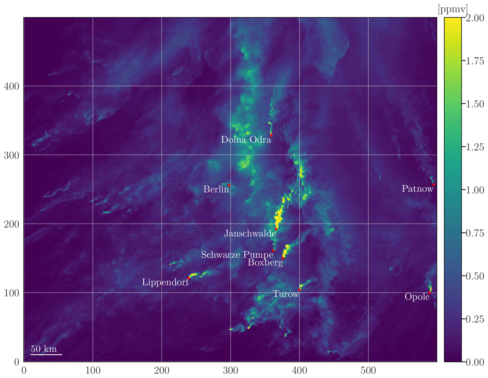
Figure 2 XCO₂ concentration map with the locations of Berlin and each considered PP within the complete SMARTCARB domain. The map consists only of the concentrations stemming from the major anthropogenic sources. Furthermore, to enhance plume visibility, as fluxes of power plants such as Jänschwalde are vastly superior to other fluxes, concentrations exceeding 2 ppmv have been capped at 2 ppmv.

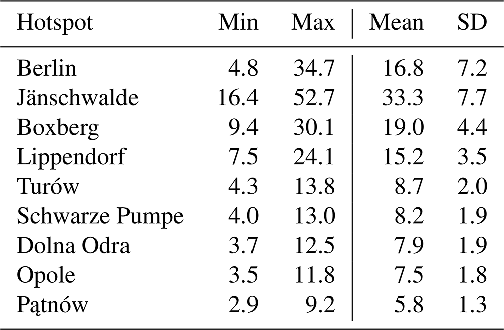
This paper only addresses the retrieval of PP emissions, although the training dataset includes the city of Berlin. More precisely, depending on the PP evaluated, the training dataset might be composed of any hotspot in Berlin, Jänschwalde, Schwarze Pumpe, Boxberg, Turów, Pątnów, Lippendorf, Opole, or Dolna Odra. The primary rationale behind prioritising the training of the model on PPs is the scarcity of cities in the dataset, which poses a challenge for the model to effectively learn and generalise for cities. However, Berlin is included in the training dataset as supplementary data to aid the model in its learning process. In the SMARTCARB dataset, the modelling of anthropogenic emissions, incorporating fixed diurnal, weekly, and seasonal cycles, was performed using the TNO-MACC III inventory (Kuenen et al., 2014). The emissions range, mean, and standard deviation of each hotspot are given in Table 1, and locations of considered PPs and Berlin are described in Table 2. Moreover, data augmentation techniques are employed to expand the database, as detailed in Sect. 4.2.1.

Table 1 Emission statistics for the PPs considered and the city of Berlin. Fluxes are in Mt CO₂ yr⁻¹.

3 Application of the segmentation model

Utilising a segmentation algorithm to incorporate plume contours as additional prior information in plume inversion may yield significant benefits. In this section, we provide a brief description and application of the CNN-based method developed in Dumont Le Brazidec et al. (2023a) that predicts plume contours in XCO₂ images. The methodology of Dumont Le Brazidec et al. (2023a) involves employing an image-to-image U-Net model, which generates images that are subsequently used as inputs for the CNN inversion model, as outlined in Sect. 4.

Apart from a few specific points, the training and model choices are similar to those of Dumont Le Brazidec et al. (2023a). A simpler encoder, with fewer neurons, is chosen, since the NO₂ fields are used as inputs to the CNN. This simplification of the problem reduces the need for a complex encoder. In addition to NO₂ and XCO₂ fields, winds are also used to assist in the XCO₂ plume contour prediction, although experiments show that the addition of these data has very little influence on the predictions. Finally, the U-Net models were designed to make predictions beyond the geographical region of their training data. Specifically, the model that learns to predict the mask of the Boxberg PP plume from an image centred at the Boxberg PP is trained on a dataset excluding the images centred at Boxberg.

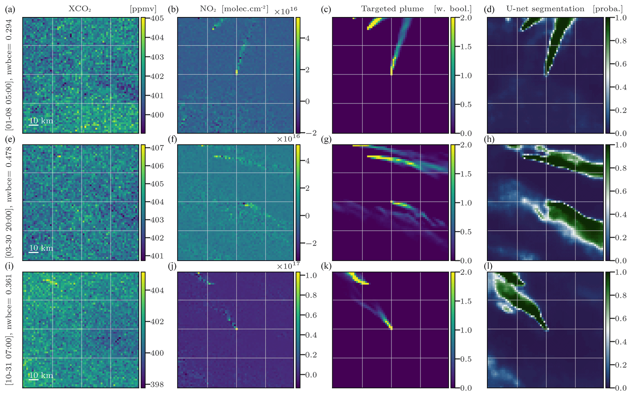
Figure 3 Examples of the U-Net CNN model application on images from the test dataset centred at Turów. The columns from left to right represent the XCO₂ images (a, e, i), NO₂ images (b, f, j), weighted Boolean plumes (c, g, k), and U-Net predictions (d, h, l) as probability maps, respectively. All times are in UTC.

In Fig. 3, we show the application of a model trained to predict the positions of Turów plumes. It was trained on pairs of fields in the regions of Boxberg, Berlin, Lippendorf, Pątnów, Jänschwalde, Dolna Odra, Schwarze Pumpe, and Opole. The first and second columns of the figure show the XCO₂ and NO₂ fields, inputs to the CNN. The third column shows the target plume as a reference point, while the fourth column shows the output of the CNN.

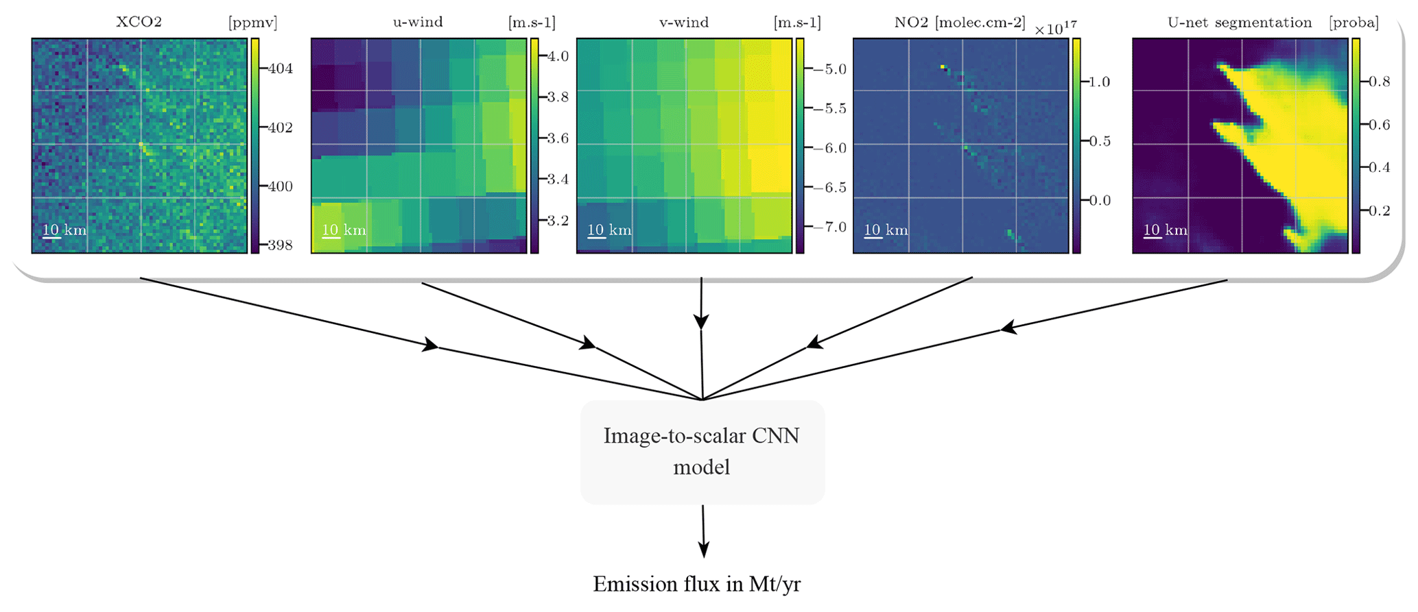
Figure 4 Various fields – XCO₂, winds, NO₂, and segmentation results – and the emissions are used by a CNN that learns to estimate the emissions associated with the central plume concealed under the background. Note that the combination of NO₂ and segmentation results as inputs is never assessed in this paper.

4 Deep learning method for the inversion of XCO₂

4.1 Inversion based on supervised learning

The inverse problem addressed here is the estimation of the CO₂ emissions accountable for the central hotspot plume observed in a given XCO₂ field image. To do so, a CNN is used, processing as input a given XCO₂ field and other additional fields and resulting in a scalar output representing the emission rate of CO₂ in Mt CO₂ yr⁻¹ at the hour corresponding to the image. The choice of representing the flux as a scalar was made for the sake of simplification, as the quality of the results is minimally impacted by the choice between targeting average, instantaneous fluxes or targeting a vector of instantaneous fluxes over the last N hours. This is due to the relatively slow hourly variation in the CO₂ emission rate of the PP. All future flux quantities are expressed in  Mt yr⁻¹. The image-to-scalar, or image regression, problem is depicted in Fig. 4. The CNN is trained using XCO₂ fields, ancillary data fields (winds, segmentation results, and NO₂), and associated emission fluxes ranging from 3 to 53 Mt yr⁻¹ across various times and targets.

4.2 CNN model and training parametrisation

In this section, we present and discuss the architecture of the model, the hyperparameters, and the learning methodology for the inversion task. In particular, the model is built from preprocessing layers and a core model. The preprocessing layers are used to augment/transform, construct, add noise, and normalise the input data before feeding them into the core model. The core model is designed to extract features from these transformed input data.

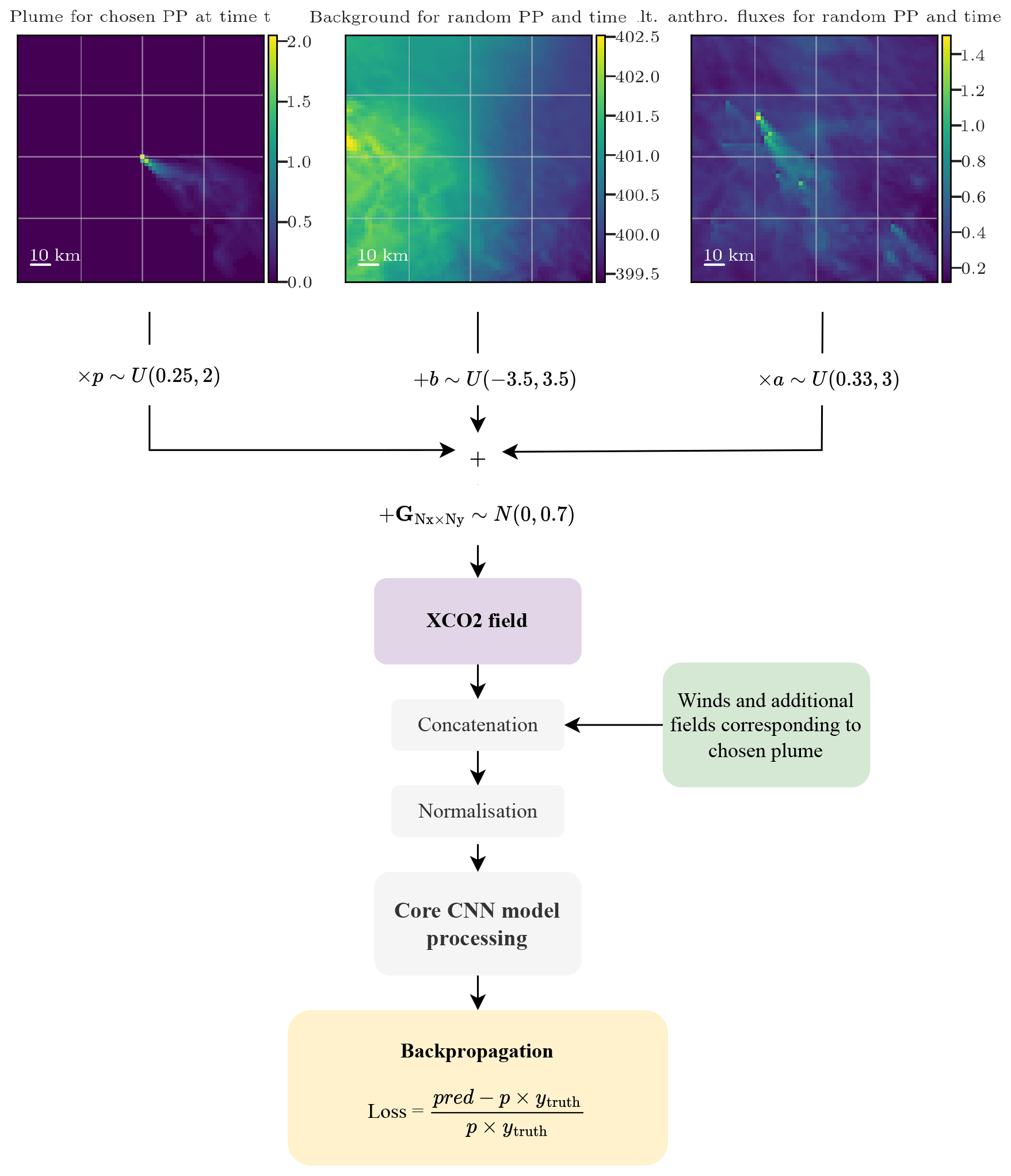
Figure 5 Description of the preprocessing layers as a sequence of six steps: (1) random choice of the XCO₂ field components, (2) scaling transformation of the components, (3) sum of the components, (4) satellite noise simulation, (5) concatenation with the additional data, and (6) normalisation.

4.2.1 Description of the preprocessing layers

The preprocessing layers consist of a six-step sequence, as presented in Fig. 5. The purpose of steps 1, 2, and 3 is to extend the initial database, thereby enhancing the model's ability to generalise to unseen data. A pair of input–output data items for training is constituted in the following way.

1. A target CO₂ plume corresponding to a PP at a time t is chosen randomly. A background must be constructed to form the XCO₂ image with this plume. This background is chosen randomly and therefore does not necessarily correspond (geographically and temporally) to the chosen target plume. It may correspond to another PP as well as to another time. Furthermore, in SMARTCARB, the background is partitioned into multiple segments. In our case, the background is constructed from two randomly and independently drawn fields: a field containing the major part of the fluxes including the biogenic fluxes and a field containing a part of the anthropogenic fluxes of the SMARTCARB domain. Finally, potential additional fields (wind, NO₂, segmentations) corresponding geographically and temporally to the chosen CO₂ plume are selected.

2. Then the following occurs.

   • The target XCO₂ plume is multiplied by a random uniform scaling factor $p\sim U(\mathrm{0.25},\mathrm{2})$. The corresponding true emissions are also multiplied: $y_{\text{truth}}^{\text{scaled plume}}=p\times y_{\text{truth}}^{\text{plume}}$.

   • A random number $b\sim U(-\mathrm{3.5},\mathrm{3.5})$ (in ppmv) is added uniformly to the main background. Extrema of this uniform distribution are chosen as approximately the standard deviation of an average XCO₂ background.

   • A random uniform scaling factor $a\sim U(\mathrm{0.33},\mathrm{3})$ is applied to multiply the field containing a part of the alternate anthropogenic fluxes.

   Anthropogenic flux scaling factors p and a are chosen so that the resultant emissions still correspond to reasonable anthropogenic fluxes.

3. The XCO₂ field is built as the sum of the target plume, background, and alternate anthropogenic fluxes field components.

4. A Gaussian noise matrix of shape 64 × 64 (equal to the image shape) ${\mathbf{G}}_{Nx\times Ny}\sim N(\mathrm{0},\mathrm{0.7})$ (in ppmv) is added to the XCO₂ field to simulate the satellite observational noise.

5. The noisy XCO₂ field is concatenated with the additional fields. If added, the NO₂ field is noised beforehand.

6. Standardisation (i.e. Z-score normalisation) is applied independently to each channel (each physical field) of the concatenated input data.

These steps are carried out exclusively during the model training phase. The different operations in this process are performed to create a more robust and diverse training dataset. To ensure an accurate assessment of the performance of the trained model, the test dataset used for the evaluation consists only of pre-constructed, physically consistent simulated data. Specifically, no scaling factors are applied and the XCO₂ fields used for testing are always constructed from geographically and temporally consistent plume and background components.

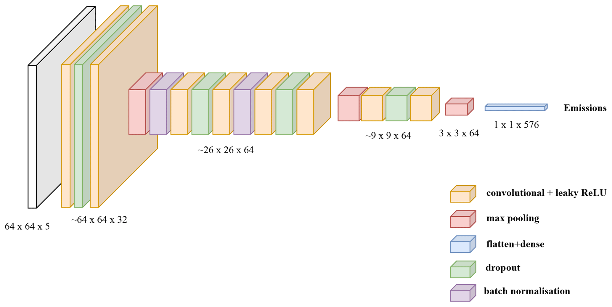
Figure 6 Description of the core CNN model, designed to extract features from the input data. The resolution given for each sequence of layers is approximate, as convolutional layers also slightly reduce the resolution.

4.2.2 Description of the core model

The chosen core CNN model, depicted in Fig. 6, is designed for image regression. It was chosen by comparing its performance with state-of-the-art models such as EfficientNet or SqueezeNet (Tan and Le, 2020). These two models are deep neural networks designed primarily for image classification tasks. They incorporate modified versions of CNN, including features such as residual connections and depth-separable convolutions, in order to improve efficiency, speed, and ease of implementation. As their initial implementation tended to overfit, we considered a smaller version with a reduced number of neurons in each layer. But even after tuning, the simpler model depicted below outperformed these more advanced models.

The chosen model takes three to four images of 64 × 64 pixels as input (which correspond to the XCO₂ field and ancillary data such as the winds). The model is constructed as a succession of convolutional, max pooling, batch normalisation, and dropout layers where the following applies:

• Convolutional layers aim to identify and extract relevant features by applying a set of learnable filters to the previous feature map. The 2D convolutional operations are applied with a filter size of 32 and a kernel size of 3 × 3.

• Max pooling layers play a key role in reducing the resolution of feature maps while retaining the essential information. This reduces the computational complexity of the network and leads to the extraction of more complex features.

• Batch normalisation layers are used to improve the stability of the network and speed up its learning process.

• Dropout layers randomly exclude a certain percentage of the neurons in the previous layer at each iteration to reduce overfitting. They are only activated during the training phase.

The output of the core model is flattened and fed into a fully connected final dense layer with a single output unit, which is activated by a leaking rectified linear unit (ReLU). In total, the CNN has approximately ∼ 186 000 parameters.

4.2.3 Training parametrisation

The training hyperparameters, such as the optimiser, learning rate, and batch size, have been determined through a combination of experimental investigation and adherence to standard practice. In accordance with customary practices, Adam's optimiser was employed with a fixed learning rate of 10⁻³ and a dropout rate of 0.2 was applied. The batch size, or number of samples before the model updates its weights, was set to 32. After analysis, to ensure model convergence, the epoch count was set to 500, which yields a total training time of approximately 4 h using an NVIDIA Quadro RTX 5000 16 GB GPU. Furthermore, the default choice of loss function employed is the mean absolute percentage error (MAPE), which emphasises proportionate deviations between emissions predictions and ground truth. This loss function is equivalent to an absolute relative error between the truth and the predictions. It should be noted that the mean absolute error (MAE) metric was used to train roughly half of the ensemble models (detailed in the subsequent section, Sect. 4.2.4) in the Lippendorf case (Sect. 5.1.1). MAE and MAPE metrics generally yielded similar performances.

4.2.4 Model ensembling

In many cases, deep learning models suffer from high levels of volatility due to their reliance on random initialisations of parameters and hyperparameter optimisation algorithms. To overcome these limitations and increase the stability of our predictions, we employed the technique of model ensembling. Specifically, for each considered configuration, we trained multiple instances of the same model architecture and parameters. This approach enabled us to produce a range of predictions that were subsequently averaged into a single estimate. To ensure sufficient convergence of these estimates, a minimum of five individual models were used for each considered configuration. Through these steps, we significantly reduced the variability observed across multiple models runs, thereby improving the accuracy and confidence in our system.

4.3 Geographical separation between the training and test datasets

We consider a strict geographical separation between the PPs of the training/validation and those of the test dataset. For example, to train a model to predict emissions from Boxberg plumes, we consider a training dataset consisting of images centred at all other available PPs except Boxberg. In this way, the model predicting Boxberg emissions never had access to the Boxberg emissions inventory.

During the training phase, to avoid overfitting or underfitting, a separate validation dataset is used to follow the model's performance using new data. In our case, the validation dataset is chosen as unseen data from the same geographical area as the training dataset.

Three distinct models are created and trained to predict emissions from three specific PPs. The target PPs are Lippendorf, Boxberg, and Turów and are selected for the following reasons:

• to obtain a diverse range of emission rates – between 7 and 24 Mt yr⁻¹, with a mean of 15 Mt yr⁻¹ and an SD of 3 Mt yr⁻¹ for Lippendorf; between 4 and 13 Mt yr⁻¹, with a mean of 9 Mt yr⁻¹ and an SD of 2 Mt yr⁻¹ for Turów; and between 9 and 30 Mt yr⁻¹, with a mean of 19 Mt yr⁻¹ and an SD of 4 Mt yr⁻¹ for Boxberg;

• to account for the potential presence of multiple plumes in the same image – the images centred at Boxberg also include plumes from Jänschwalde, Schwarze Pumpe, and Turów, which sometimes overlap;

• because their emission rates are at neither the highest nor the lowest extremes (Boxberg was selected over Jänschwalde because Jänschwalde has the highest emission levels in our dataset, potentially placing it outside the training distribution);

• due to their positioning away from the boundaries of the SMARTCARB domain. These PPs are less affected by border conditions – as shown in Fig. 1, Pątnów or Opole are close to the borders and are influenced by border conditions.

Although these models differ in terms of the training datasets used, they all share the same architectural framework, including hyperparameters, CNN structure, and preprocessing layers. The objective behind creating these models is to demonstrate the effectiveness of the architectural framework, laying the groundwork for a universal model based on this architecture and capable of generalising across future PPs. It is important to note that while the test dataset from one experiment appears in the training dataset of another, each experiment was conducted independently. The model tuning was not influenced by the results obtained with the test datasets. In particular, the selection of the hyperparameters such as the learning rate was made before the model training.

4.4 Alternative method for comparison

The accuracy of our inversion method is compared to the cross-sectional flux (CSF) method implemented in the Python library for data-driven emission quantification (ddeq¹). The CSF method was recently compared with other state-of-the-art methods and shows similar accuracy than other well-performing methods (Hakkarainen et al., 2023). This method consists in

• detecting the plume and extracting it from the background, whereby NO₂ fields are used to help in the detection;

• dividing the plume into a series of horizontal slices of known areas and heights;

• estimating the line densities of CO₂ by fitting Gaussian curves to the CO₂ and NO₂ concentrations within each slice;

• inferring the CO₂ fluxes as the product of the line densities and the wind speed at the sources;

• deriving the total emission rate by multiplying the flux estimation and the area of each slice and then averaging all downstream fluxes.

The CSF method is limited by the need for accurate estimation of the effective wind (Kuhlmann et al., 2020a). Two separate wind estimates have been considered: the first derived from an average of the 37 lower levels of ERA5 data and the second corresponding to the wind at 100 m. The first estimate was chosen because of its superior performance.

5 Application: inversion of three power plants and model interpretation

In this section, we study the performance of a trained CNN under the conditions exposed in Sect. 4:

• Firstly, various ensembles of models with different sets of inputs are evaluated using the Lippendorf PP in Sect. 5.1.1, the Turów PP in Sect. 5.1.2, and the Boxberg PP in Sect. 5.1.3. In each configuration, the training, validation, and test datasets involve 25 152, 4608, and 6289 images, respectively.

• Secondly, we investigate how the assimilation of segmentation fields or NO₂ affects the CNNs. Afterwards, since overfitting arises in certain configurations, discussions and partial solutions to this issue are proposed.

• Thirdly, we propose to interpret the CNNs using a gradient-based technique and by permuting the input features.

5.1 Inversion of plumes' performance

We study the performance of various CNN model ensembles in predicting the emissions of the Lippendorf, Turów, or Boxberg PPs. More precisely the following applies:

• Three model ensembles are trained on Berlin, Jänschwalde, Schwarze Pumpe, Boxberg, Turów, Pątnów, Opole, and Dolna Odra and are tested on Lippendorf.

• Three model ensembles are trained on Berlin, Jänschwalde, Schwarze Pumpe, Boxberg, Lippendorf, Pątnów, Opole, and Dolna Odra and are tested on Turów.

• Three model ensembles are trained on Berlin, Jänschwalde, Schwarze Pumpe, Turów, Lippendorf, Pątnów, Opole, and Dolna Odra and are tested on Boxberg.

Lippendorf typical emissions fall between those of low-emission PPs (such as Dolna Odra or Turów) and those of high-emission PPs (Boxberg, Jänschwalde). Turów emissions range between 4 and 14 Mt yr⁻¹, which is similar to PPs like Opole. This implies that most Turów CO₂ plumes are hidden under the background. The last-studied PP is Boxberg, which is characterised by high emissions and the presence of other PPs in the vicinity, which entails the presence of other high-SNR plumes.

For each of the three target PPs, three model ensembles are trained. The input data for the first model ensemble are the XCO₂ field and the wind fields u and v. The second and third model ensembles use the same three base fields and the output of the segmentation model or the NO₂ field, respectively, as fourth input. In the following, for simplicity, these ensembles of CNN models will be referred to simply as “models”.

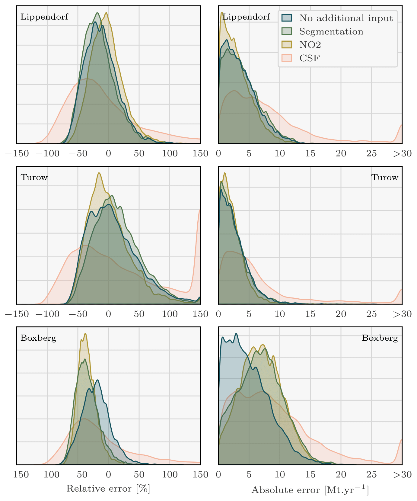
Figure 7 Density plots of the signed relative and absolute error between the predicted and the true Lippendorf emissions. Four sets of predictions are considered, corresponding to the three CNN models with three different sets of inputs and the CSF method. Each CNN model is trained with the XCO₂ field and the winds as inputs. Two of the models additionally assimilate the NO₂ field or the predictions of the segmentation model. Predictions with absolute relative errors greater than 150 % or absolute errors greater than 30 Mt yr⁻¹ were set to ± 150 or 30 to increase visibility. Of the CSF method predictions, 3 % are missing. Those predictions correspond to Lippendorf plumes superimposed onto other plumes, where the CSF method cannot be applied.

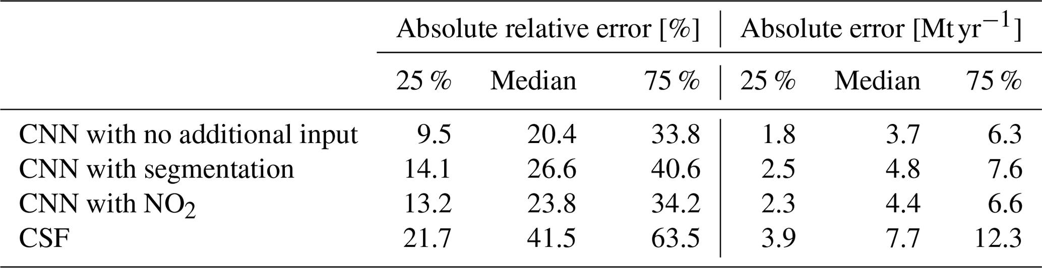
Table 2 Absolute relative and absolute error statistics between predicted and true emissions for CNN models with various inputs and applied to various target PPs and the CSF method.

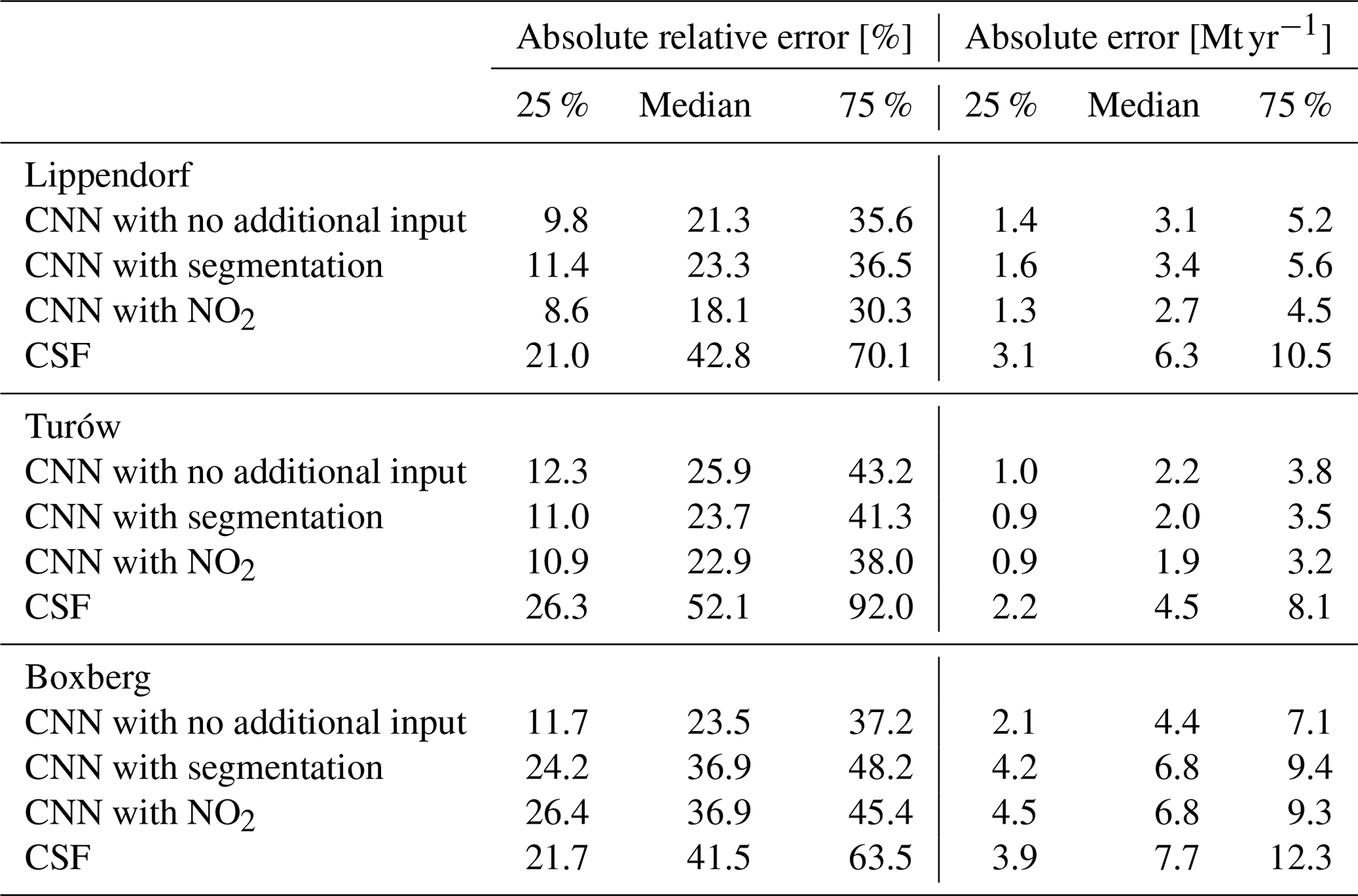
Kernel density estimation (KDE) plots over the 6289 images of the test dataset are drawn in Fig. 7, comparing with relative and absolute metrics the true emission rates and the predictions of the four models for each PP. While Fig. 7 employs signed relative error to assess prediction bias in the CNNs, Table 2 and the majority of the analysis rely on absolute relative error. KDE is a non-parametric statistical technique that estimates the probability density function of a continuous random variable by smoothing its observed data points using a kernel function. The three first ensembles of predictions consist of those of the trained CNNs, and the fourth corresponds to the CSF method application. The main statistics corresponding to these KDE plots are summarised in Table 2.

5.1.1 Lippendorf plumes' inversion

As reported in Table 2, the utilisation of the CNN approach yields remarkably accurate predictions of Lippendorf emissions compared to the CSF method. The performance of all three CNN models shows a median absolute relative error of approximately 20 % and a median absolute error of around 3 Mt yr⁻¹ (the average emissions for Lippendorf are 15.2 Mt yr⁻¹). In comparison, the CSF method exhibits a higher median absolute relative error performance of around 40 %, and the absolute error performance is approximately double, at 6 Mt yr⁻¹. The CNN results are reliable, as the majority of errors are concentrated below 10 Mt yr⁻¹ or 50 %, with very few exceeding 100 %. This indicates that the models provide trustworthy estimates, with a relatively small margin of error.

5.1.2 Turów plumes' inversion

The CNN approach produces highly accurate predictions for the low-SNR Turów plumes, exhibiting similar performance to the results obtained in the Lippendorf case. The three models yield a median absolute relative error performance of approximately 25 % and a median absolute error performance of around 2 Mt yr⁻¹. The results can be considered reliable: 75 % of the results fall below a threshold of 4 Mt yr⁻¹. By contrast, the CSF method exhibits a median absolute relative error performance of approximately 50 %–55 % and an absolute error more than 2 times larger. The inclusion of segmentation or NO₂ fields has a noticeable, albeit not significant, impact on the model's performance, resulting in an improvement on the order of a 10th of 1 Mt yr⁻¹. Notably, the addition of the NO₂ field appears to have a slightly greater impact compared to the inclusion of segmentation fields. This implies that when applying the model that assimilates the segmented XCO₂ fields (with the assistance of the NO₂ fields), there is a potential loss of information for the NO₂ fields compared to using the model directly assimilating the NO₂ fields. The observed phenomenon could be a result of potential overfitting when employing the segmentation model, as it is trained on the same dataset as the inversion model. Consequently, the segmentation predictions on the training dataset are typically superior to those on the test dataset. This discrepancy can lead to an over-reliance on the segmentation fields, subsequently causing overfitting.

5.1.3 Boxberg plumes' inversion

In contrast to the inversion results obtained for Lippendorf and Turów PPs, there is a significant variation in Boxberg plume inversion performance. A CNN only trained with XCO₂ and u and v winds demonstrates strong performance, comparable to that of the models estimating Lippendorf and Turów emissions. The median absolute relative error performance is approximately 20 %–25 %, and the median absolute error performance is around 4 Mt yr⁻¹. The CSF method exhibits a median absolute relative error performance of around 40 % and an absolute error performance close to 8 Mt yr⁻¹. But both models with segmentation or NO₂ fields show a significant decline in performance, which contradicts our expectations. This phenomenon can be attributed to overfitting and is examined in detail in Sect. 5.2.2.

5.1.4 Cross-sectional flux method results

The CSF results align with the findings reported in Kuhlmann et al. (2021) and Hakkarainen et al. (2023). Other methods, such as the light cross-sectional fluxes technique, might yield predictions with absolute relative errors reduced by 5 % to 10 % (Hakkarainen et al., 2023). A notable constraint of the CSF method is that it hinges on the estimation of the effective wind speed inside the plume. Under ideal circumstances, the effective wind speed should be estimated using the wind profile, weighted by the CO₂ concentration profile, but in practical applications, estimating this profile presents a substantial challenge. In a separate experiment, the CSF method was utilised based on a reduced dataset (compared with that used to study the CNN results). Among other changes, this dataset considers only the CO₂M overpass, or excludes the plume overlaps processed by the CNN. In this experiment, the exact emission profile used to simulate the COSMO-GHG fields of SMARTCARB was used to compute the effective wind. This methodology resulted in a median absolute error of around 4 Mt yr⁻¹, thereby indicating that the effective wind estimation significantly contributes to the errors associated with the CSF method.

5.2 Result analysis

This section presents an analysis of the results from the preceding section, Sect. 5.1. It involves examining the trained models, or new models trained under the same configuration, across various datasets, including the test dataset. It is important to note that these analyses were conducted after obtaining the previous section's results and thus did not influence, for example, the choice of model architecture or hyperparameters.

5.2.1 Study of the addition of the segmentation and NO₂ fields

Interestingly, the model designed to invert the Lippendorf plumes does not yield more accurate emission estimates when using segmentations as inputs, compared to the model without segmentations. One possible reason for this lack of improvement is that the Lippendorf segmentation fields are inadequate. The segmentation model assimilates NO₂ fields to segment the CO₂ fields, and the presence of multiple alternative NO₂ plumes in the NO₂ fields hinders the segmentation model's ability to accurately delineate the contour of the Lippendorf CO₂ plume. However, the incorporation of the NO₂ field as inputs slightly increases the quality of the predictions made by the new CNN model. One hypothesis to explain the error discrepancy between the model utilising NO₂ and the one using segmentation fields is the segmentation model not capturing NO₂ or CO₂ plume amplitude variations. Precisely, the segmentation model does not discriminate between plume pixels with high amplitude and those with low amplitude. Consequently, if the NO₂ images are of poor quality due to the presence of numerous alternative NO₂ plumes, the segmentation model will struggle to distinguish the main plume accurately. Taking into account these segmentation fields that do not distinguish the background plumes in the test dataset results in a degradation of the predictions.

Regarding the benefits brought by the integration of NO₂ fields, their essential contribution is their facilitation of the plume segmentation, rather than a direct enabling of inversion based on the NO₂ levels alone. Indeed, as stated in Sect. 4.2.1, the NO₂ plumes are not scaled like CO₂ plumes. To further investigate this, it is possible to verify this hypothesis by modifying the scaling of the plume in the NO₂ fields. In Fig. 8 we draw the relative absolute error of the model at testing stage when taking as inputs scaled NO₂ fields by a constant factor in [0,3]. The CNN model exhibits its highest performance within the scaling range of 1.0 to 1.3. As expected, performances gradually decrease for scaling below 1 and above 1.3. However, intriguingly, the model still achieves remarkably satisfactory scores for scalings ranging from 0.5 to 1.75. Notably, these scores outperform those of the CNN models without the NO₂ field as input. If the model were utilising the amplitude of the NO₂ field as a predictor, deeply inaccurate results could be expected for scalings of 0.5 or 1.5. However, the graph contradicts this assumption, strongly suggesting that the amplitude of the NO₂ field is not employed as a predictor by the model. Instead, it is likely that only the contour of the NO₂ plume and the ratios between different parts of the plume serve as predictors. In essence, the model's reliance on the NO₂ field for predictions appears to be based on the contour of the plume and the relative proportions of its various components, rather than on the absolute amplitude of the NO₂ field values. Finally, the model's inability to accurately estimate emissions for scaling factors exceeding 2 can be attributed to the unprecedented and extreme values that NO₂ plumes can reach, which lie beyond the range of what the model has been trained on.

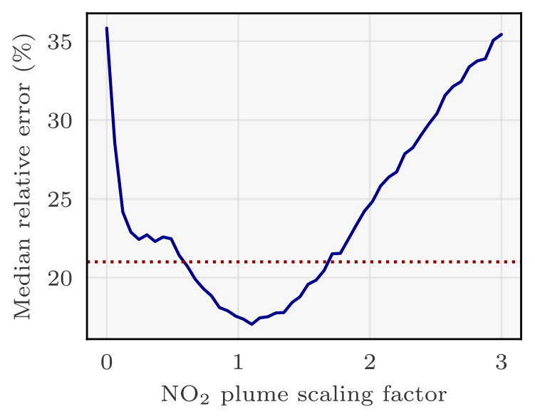
Figure 8 Effect of scaling the NO₂ plume of Lippendorf inputs on the performance of the CNN model. The x axis corresponds to the scaling of the NO₂ plume: 1 corresponds to the original plume and 0 to no plume. The y axis corresponds to the median absolute relative error of the CNN model evaluated for the given scaling of the NO₂ plumes. The CNN model is the same for each scaling (each tick of the x axis) and corresponds to the CNN model having obtained the best absolute relative error score. The dotted red line approximately corresponds to the median absolute relative error of a model not learning with NO₂ fields.

5.2.2 Overfitting investigation

To understand the reasons behind the deviations between predictions and actual values, we conducted an analysis of the residuals in Fig. 9. This examination, which focuses on the disparities between predicted and true emissions, reveals a substantial underestimation of the actual Boxberg emissions by the model incorporating NO₂ or segmentation fields.

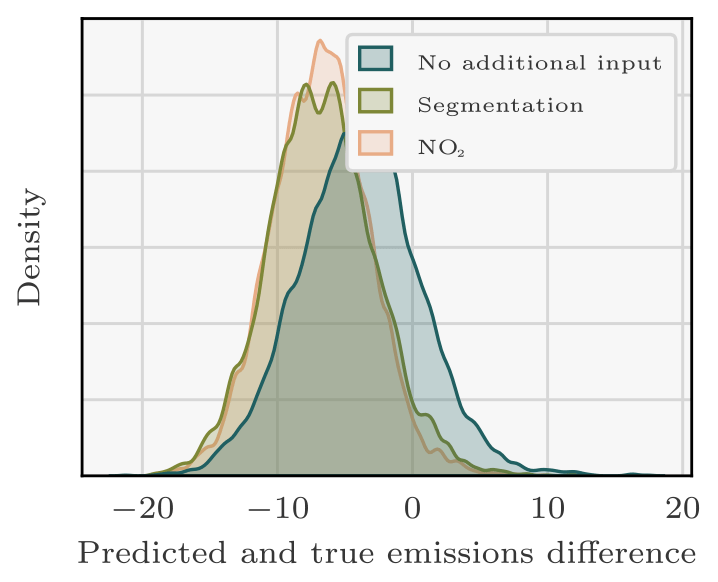
Figure 9 Residual density between the true emissions of the Boxberg PP and the predictions of the CNNs.

This observation suggests an overfitting issue (Zhang et al., 2022), since the majority of PPs used to train the model exhibit lower emission rates compared to Boxberg (six out of seven: Schwarze Pumpe, Lippendorf, Turów, Pątnów, Opole, and Dolna Odra). The low absolute relative error observed in the training dataset of the models with NO₂ or segmentation fields, as depicted in Fig. 10, further substantiates concerns regarding overfitting. An overfitted model tends to learn features that are overly tailored to the specifics of the training dataset. Consequently, when presented with images from the test dataset with slightly different features, the model struggles to generate accurate predictions.

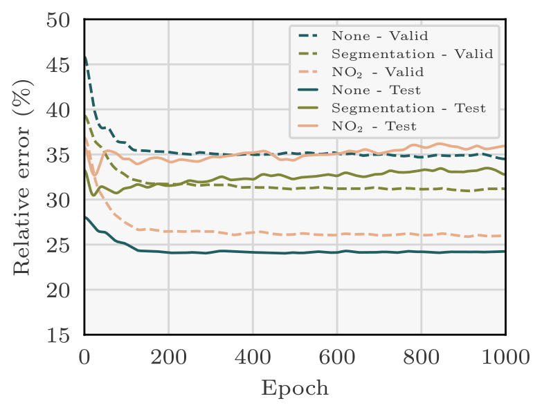
Figure 10 Evolution during training of the validation and test relative errors between the true emissions of Boxberg and the predictions of the CNNs. Specifically, for the needs of this experiment, new models are trained and employed to predict the emissions corresponding to the validation and test fields at each epoch. Three models are considered: each is trained with the XCO₂ field and the winds as inputs. Two of the models additionally assimilate the NO₂ field or the predictions of the segmentation model. The validation error decreases monotonically with the number of epochs, while the test error does not, which suggests overfitting of the model.

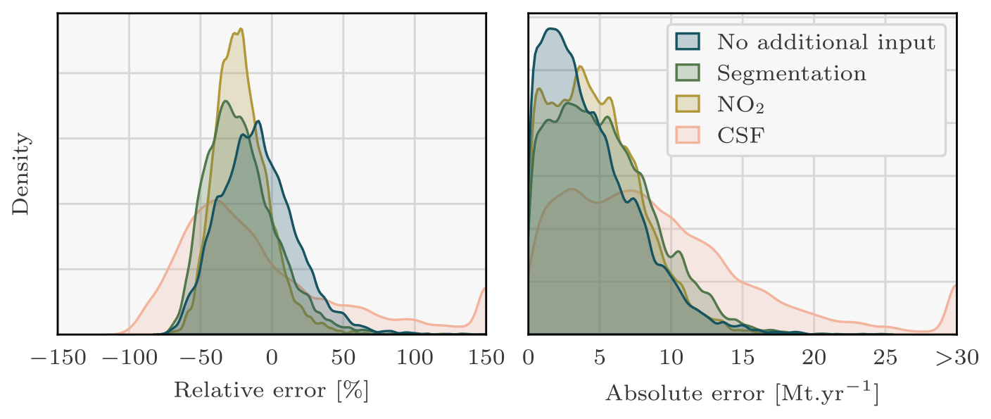
Figure 11 Density plots of the relative and absolute error between the predicted and the true emissions. Four sets of predictions are considered, corresponding to the three CNN models with three different sets of inputs and the CSF method. Each CNN model is trained with the XCO₂ field and the winds as inputs to a dataset composed of Berlin, Jänschwalde, Lippendorf, Turów, and Opole. Two of the models additionally assimilate the NO₂ field or the predictions of the segmentation model. Predictions with absolute relative errors greater than 150 % or absolute errors greater than 30 Mt yr⁻¹ were set to 150 or 30 to increase visibility. Of the CSF method predictions, 15 % are missing. Those predictions correspond to Boxberg plumes superimposed onto other plumes, where the CSF method cannot be applied. A modified dataset is used to avoid overfitting.

Table 3 Relative and absolute error statistics between predicted and true Boxberg emissions for three CNN models (assimilating three different sets of inputs) and the CSF method. A modified dataset is used to avoid overfitting.

Our hypothesis is that the model specifically overfits the low-emission PPs, which can be attributed to the information gained through the use of NO₂ or segmentation fields. When provided with new images, the model fails to recognise the new features and consequently yields predictions that align more closely with the training dataset, which predominantly consists of emissions from the low-emission PPs. The failure to recognise new features is due to the incorporation of the NO₂ field as inputs. The model's ability to learn highly specific features is limited when no additional input is provided. Conversely, when the model incorporates the NO₂ field, it gains access to more information and can acquire more intricate features. Consequently, the model's capacity to generalise worsens in the latter case.

Next, we examine the performance of a new ensemble of models trained on a more balanced dataset, achieved by removing three out of the five low-emission PPs from the original dataset. The new dataset is composed of Berlin, Jänschwalde, Lippendorf, Turów, and Opole, i.e. of two medium- or high-emission PPs and two low-emission PPs and Berlin. Furthermore, the choice of the factor scaling the plumes during training (see Sect. 4.2.1) varies depending on the ensemble member considered (see Sect. 4.2.4). Specifically, the uniform distribution is defined with a minimum scaling factor of 0.25 or 0.5 and a maximum scaling factor of 2 or 3. Once more, we examine the outcomes for three models obtained from ensembling, as depicted in Fig. 11, and summarise them in Table 3.

The three CNN models demonstrate very good performance, although the inclusion of NO₂ or segmentation fields still leads to a degradation in results, albeit to a lesser extent than in Sect. 5.1.3. For example, the median absolute relative error for the CNN with NO₂ as additional input is 23.8 %, compared to 36.9 % in Sect. 5.1.3. On the one hand, the median absolute relative error of the CNN model trained on NO₂ and wind fields stands at approximately 20 %, while the median absolute error remains below 4 Mt yr⁻¹. On the other hand, the degradation of the results when adding the NO₂ or segmentation fields can still be regarded as overfitting. The model learns features from NO₂ or segmentation fields that are not general enough to cover the case of Boxberg. Furthermore, it fails to acquire compensatory generalisable features such as in the case of Turów, where the model probably gains information about the plume contour from the NO₂ field, which is not straightforwardly apparent in the Turów XCO₂ field.

5.3 Interpretation of the CNN inversion models

In the two following sections, we introduce and apply two methods to gain a deeper understanding of the behaviour and decision-making processes of the CNNs discussed in this paper. These methods offer valuable insights into the significance of input features in the predictions made by the CNNs:

• The integrated-gradient method allows us to examine the importance of individual pixels across channels.

• The feature permutation method enables us to assess the importance of the channels, i.e. the fields used as inputs.

5.3.1 Gradient-based study of the pixels

The integrated gradients method is a gradient-based method for the interpretability of neural networks that enables the assessment of pixel importance in CNN prediction. The method calculates the sensitivity of a model's predictions to input features (here pixels), assigning relevance scores to them. By analysing how changes in the input pixels affect the model's output, the method provides insights into the importance of each pixel in the decision-making process.

One unique aspect of this gradient-based method is that the scores it assigns are relative to a baseline. More precisely, these scores are computed as integrated gradients along a linear interpolation from a blank image to the input.

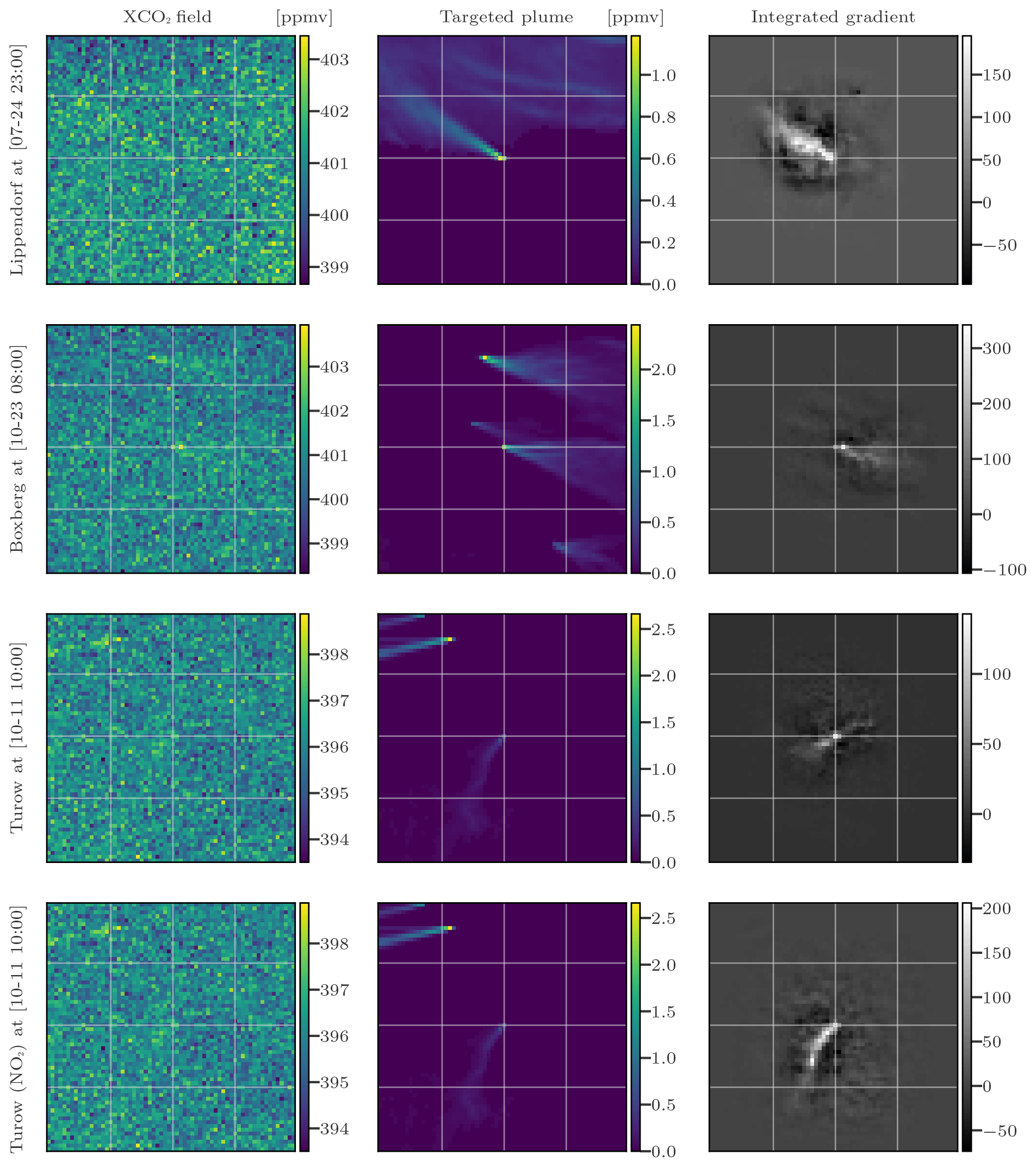
Figure 12 Evaluation of four CNN models using the integrated-gradient method with four input sets. Columns 1, 2, and 3 represent the XCO₂ field, the corresponding XCO₂ plume, and the integrated gradient between the model predictions and the inputs, in that order. The rows represent the four models and corresponding test fields.

In Fig. 12, we apply the integrated-gradient approach to study four different models specific to various sources. The first and second models are built to invert the emissions from Lippendorf (see Sect. 5.1.1) and Boxberg plumes (see Sect. 5.1.3), respectively, whereas the last two models target Turów plumes (see Sect. 5.1.2). The first three models only use the XCO₂ field and the winds as inputs, whereas the fourth model considers an additional input, the NO₂ field. To apply the integrated-gradient method, a random plume from the target PP is selected for each model. Columns of Fig. 12 represent the XCO₂ field, the corresponding XCO₂ plume, and the integrated gradient between the model predictions and the inputs.

In order to simplify the analysis, we choose the model that exhibits the best performance using the test dataset, rather than using the ensemble of models. It is worth noting that such a model yields similar performances to the ensemble of models.

The integrated-gradient technique reveals that the CNN model learns to estimate the emissions of a source based on the pixels of the plume from this source. In the first row, we examine a plume from Lippendorf PP. The integrated-gradient technique identifies the most important pixels, which correspond to the plume pixels. This indicates that if the pixels associated with the plume were to deviate, the estimated flux rate would be significantly affected. This demonstrates that the CNN model effectively makes inferences from the crucial parts of the image. In the second row, we focus on an image centred at Boxberg. The gradients reveal that the model concentrates exclusively on the Boxberg plume in the centre, disregarding the other plumes when inferring the emissions of the Boxberg PP. In the third row of the figure, we examine a plume from the Turów PP. Although the precision is lower compared to the Lippendorf or Boxberg cases, the pixels in the general direction of the Turów plume are the main ones used to estimate the emissions. In the fourth row, we display the gradients associated with the same Turów image but for a model trained with NO₂ fields as additional inputs. In this case, the model clearly identifies the pixels corresponding to the plume as critical, as indicated by the amplitude and contour of the gradients. This reinforces the hypothesis that the improved estimation of Turów emissions when the model is trained with NO₂ fields can be attributed to the enhanced assessment of the plumes.

In conclusion, the model consistently identifies the target emission plume situated at the image's centre, indicating it implicitly understands the relationship between the plume and targeted emissions.

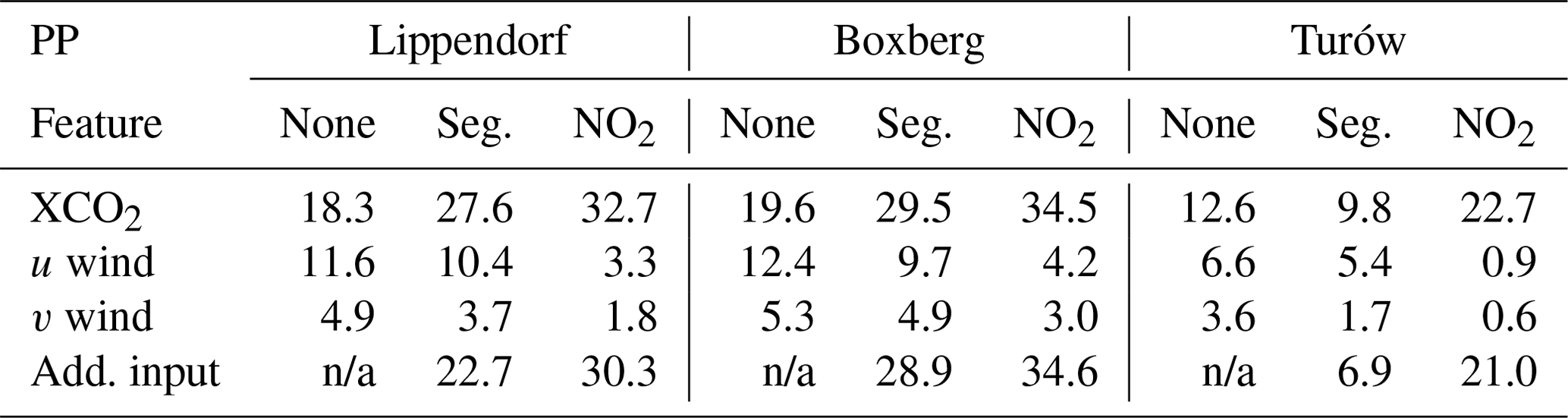
Table 4 Evaluation of the degradation in the average absolute relative error of the model when the corresponding feature is permuted. Each column corresponds to a model, and each row corresponds to a permuted feature. For example, we estimate the emissions corresponding to Boxberg plumes with the CNN model trained with the XCO₂ field, the winds, and no additional input. We then estimate the degradation of the predictions of this model on the test dataset with the u wind fields permuted: the degradation in the absolute relative error is 12.4 %. Seg. is for segmentation. Add. input corresponds to either the “None”, “NO₂”, or “Seg.” fields depending on the column considered.

n/a: not applicable.

5.3.2 Feature permutation analysis

Feature permutation is a technique used to determine the importance of input channels used in a model (Molnar, 2022). As input variables used here are not independent, the interpretation of the following permutation analysis should be taken with caution. The principle is to (i) permute the values of a feature (e.g. exchange the u wind field corresponding to an XCO₂ image with another random u wind field) and (ii) use the model to predict emissions for the given input, which includes the XCO₂ field, other associated inputs, and the random u wind field. By comparing the performance of the model using the original dataset with the performance on the permuted dataset, we can measure the impact of each feature on the performance of the model. The more the permutation of a feature affects the performance of the model, the more important that feature is. In Table 4, we present the outcomes of the permutation of the features for nine ensembles of models (for each PP and each ensemble of inputs considered). Each entry in the table represents the degradation in the average absolute relative error of the model (associated with a specific column) when the corresponding feature is permuted (related to the respective row).

We can formulate hypotheses regarding several groups of cells in Table 4.

• Comparison of the first row with the others shows that the XCO₂ feature consistently holds (or shares) the highest importance among other features.

• Examining the second and third rows reveals a pattern where the u wind seems to have a more significant influence on the inversion process compared to the v wind. This might be due to the bigger variance of u (∼ 51 m² s⁻²) comparing to v (∼ 19 m² s⁻²): u is the dominant wind in this situation.

• The XCO₂ field input permutation seems to have a lower impact for the CNN targeting Turów (12.6 % in absolute relative error degradation compared to 18.3 % and 19.6 % for Lippendorf and Boxberg).

• The importance of the XCO₂ feature differs for models with different inputs: specifically, the XCO₂ feature importance increases when additional data are used. For example, the XCO₂ feature permutation degrades the performance of the model by 32.7 % when NO₂ is used and by 18.3 % when no additional input is used. This observation is consistent with the overfitting tendency of the CNN models when trained with NO₂ fields. When confronted with inconsistent data (non-corresponding XCO₂ and NO₂ fields), the acquired complex features of the model exhibit a total absence of correspondence with these inputs. As a consequence, the model predicts nonsensical emissions.

• The wind inputs systematically hold greater importance in the model without additional input, followed by a relatively diminished importance in the model with segmentation fields, and finally, it exhibits the least significance in the model with NO₂ fields. This suggests that the inclusion of NO₂ fields is more advantageous for inversion compared to segmentation fields. Furthermore, it indicates that the winds compensate for the absence of additional data.

6 Discussions and limitations

The approach developed in this paper carries certain limitations: firstly, it focuses exclusively on European PPs, which raises questions about its generalisability to PPs in other regions with different climatic conditions. Secondly, the study emphasises the importance of a balanced dataset, as highlighted by Sect. 5.2.2, and the need to be able to identify and address potential overfitting issues. It should also be noted that the study did not specifically investigate outliers such as PPs with exceptionally high emission rates. Despite incorporating plume scaling strategies, the model may struggle to generalise to such outliers. A last limitation is the absence of a zero-emission source in the dataset. However, the inclusion in the training dataset of very low-emission power plants and of a plume scaling approach generating near-zero-emission plumes indicates that incorporating zero-emission cases would likely not markedly change the outcomes.

In terms of future research, several areas should be explored such as the challenge posed by clouds. In this respect, CNNs can be trained to ignore missing data caused by cloud cover and to make effective use of the available data. Another aspect to consider is the presence of noise in CO₂M data. While Gaussian noise may not pose significant issues if the satellite noise exhibits structured patterns, it would become crucial to develop robust noise modelling techniques to enable CNNs to accurately distinguish and remove such noise. Furthermore, in real-world applications, models trained on synthetic datasets may face challenges when applied to real datasets due to differences in data distribution. Strategies such as importance weighting, specific data augmentation techniques, transfer learning, or active learning methods may be necessary to account for these differences and ensure reliable performance. Finally, the method could be modified to extract CO₂ emissions from plume imagery at more detailed scales, necessitating the use of resource-intensive large-eddy simulation (LES) models.

7 Conclusions and perspectives

The future availability of CO₂ satellite imagery, through missions such as the Copernicus CO₂ Monitoring (CO₂M) mission, heralds new opportunities and challenges for the evaluation of local CO₂ emissions. Emissions can certainly be retrieved from CO₂ plumes of hotspots in the satellite images. But the emission estimation is hindered by two primary obstacles: plumes with a low signal-to-noise ratio which cannot be extracted straightforwardly from the background and uncertainties in the transport or dispersion processes which hampers the assessment of the emissions from the plumes.

In this work, we assess the ability of convolutional neural networks (CNNs) to invert a plume from satellite imagery using simulated XCO₂, NO₂, and wind fields with similar characteristics to the future CO₂M images. The fields used to train and evaluate the CNNs are based on the SMARTCARB dataset and possess the same resolution, satellite noise level and ancillary data availability as the future CO₂M images. Each synthetic XCO₂ image encompasses the anthropogenic plume from at least one power plant, a background arising from other biogenic and anthropogenic fluxes, and random Gaussian noise intended to simulate the errors inherent in satellite instruments. But the model evaluation was conducted using simulated data. This approach does not account for all the challenges that real satellite images present, specifically issues related to cloud cover and systematic error patterns due to surface reflectance and the aerosol dependency of retrievals.

Our source emission estimation model is an image-to-scalar CNN model, which infers from the full XCO₂ field a flux rate estimation of the anthropogenic emission corresponding to the plume. The first layers of the model consist of preprocessing steps which transform the input data during the training time, in particular by adding noise and by scaling the plume and emission rate. The core model is a CNN composed of approximately 200 000 neurons divided into convolutional, max pooling, dropout, and batch normalisation layers.

We strongly suggest that the design of a “universal” CNN, trained on a small power plant subset and highly accurate when applied to all of them, is possible. To do so, we evaluate the model's ability to generalise to unobserved images from another region. Explicitly, three CNN models trained on different datasets but sharing the exact same structure (hyperparametrisation, architecture, etc.) are tested on plumes from three sources: Boxberg, Lippendorf, and Turów. The training/validation dataset for each CNN is restricted to a dataset consisting of all other power plants except their target. The CNNs are highly accurate in each case, and the addition of NO₂ fields often improves the results slightly. Precisely, the median absolute relative errors for the CNN models are on average close to 20 %–25 %. Moreover, the median absolute error is generally half that obtained with the CSF method, which is an alternative and state-of-the-art inversion approach. This strongly suggests that it is possible to build a universal neural network (which can generalise to all targets) using this methodology.

Using interpretability tools, we demonstrate that the predictions made by the CNNs are grounded in the physically meaningful components of the features. The integrated-gradient method shows that the CNNs learn to predict the emissions corresponding to a plume from the pixels making up the plume. The feature permutation technique highlighted several aspects of the models, such as the expected high importance of the XCO₂ fields compared to the ancillary data used.

Future prospects of the CNN plume inversion method from satellite images encompass the challenges of clouds, cities, and real satellite images. Concretely, the method should be able to handle missing data caused by clouds. Additionally, the CNN approach should incorporate the second important category of hotspots: cities. Finally, the method should be tested on real satellite data once they become available.