the Creative Commons Attribution 4.0 License.
the Creative Commons Attribution 4.0 License.
 | 29 Feb 2024
Assessment of climate biases in OpenIFS version 43r3 across model horizontal resolutions and time steps
Abhishek Savita
Joakim Kjellsson
Robin Pilch Kedzierski
Mojib Latif
Tabea Rahm
Sebastian Wahl
Wonsun Park
We examine the impact of horizontal resolution and model time step on the climate of the OpenIFS version 43r3 atmospheric general circulation model. A series of simulations for the period 1979–2019 are conducted with various horizontal resolutions (i.e. ∼100, ∼50, and ∼25 km) while maintaining the same time step (i.e. 15 min) and using different time steps (i.e. 60, 30, and 15 min) at 100 km horizontal resolution. We find that the surface zonal wind bias is significantly reduced over certain regions such as the Southern Ocean and the Northern Hemisphere mid-latitudes and in tropical and subtropical regions at a high horizontal resolution (i.e. ∼25 km). Similar improvement is evident too when using a coarse-resolution model (∼100 km) with a smaller time step (i.e. 30 and 15 min). We also find improvements in Rossby wave amplitude and phase speed, as well as in weather regime patterns, when a smaller time step or higher horizontal resolution is used. The improvement in the wind bias when using the shorter time step is mostly due to an increase in shallow and mid-level convection that enhances vertical mixing in the lower troposphere. The enhanced mixing allows frictional effects to influence a deeper layer and reduces wind and wind speed throughout the troposphere. However, precipitation biases generally increase with higher horizontal resolutions or smaller time steps, whereas the surface air temperature bias exhibits a small improvement over North America and the eastern Eurasian continent. We argue that the bias improvement in the highest-horizontal-resolution (i.e. ∼25 km) configuration benefits from a combination of both the enhanced horizontal resolution and the shorter time step. In summary, we demonstrate that, by reducing the time step in the coarse-resolution (∼100 km) OpenIFS model, one can alleviate some climate biases at a lower cost than by increasing the horizontal resolution.
- Article
(8022 KB) - Full-text XML
- BibTeX
- EndNote


In the last few decades, atmosphere–ocean general circulation model (AOGCM) simulations from the Coupled Model Intercomparison Project (CMIP) have been widely used to study the internal climate variability and the climate response to external forcings, such as increasing atmospheric greenhouse gas concentrations, causing global warming. These simulations, however, suffer from long-standing biases (Bayr et al., 2018; Flato et al., 2014; Gates et al., 1999; Kim et al., 2014; Zhou et al., 2020), which lead to significant uncertainties in short-term and long-term climate projections and potential ecosystem impacts (Athanasiadis et al., 2022; Couldrey et al., 2021; Meehl and Teng, 2014; Meng et al., 2022). These biases can arise from a variety of sources, including inaccurate representation of physical processes, poor initialization of model conditions, or inadequate representation of the Earth's topography and land cover.
Simulations using atmospheric general circulation models (AGCMs) from the Atmosphere Model Intercomparison Project (AMIP), a part of CMIP, are used to study the internal variability of the atmosphere. The AGCMs are less complex than the AOGCMs as the former are constrained by observed sea surface temperature (SST) and sea ice concentration (SIC). Despite being constrained by the observations, the AGCMs also exhibit biases (e.g. Gates et al., 1999), and some of these biases have persisted for over several phases of AMIP (He and Zhou, 2014). The biases in AGCMs are largely due to the fact that many unresolved processes, such as atmospheric convection, precipitation, clouds, cloud microphysical and aerosol processes, boundary layer processes, and interactions between the land surface and hydrologic processes, have to be included in a parameterized form in the coarse-resolution model (Ma et al., 2022). The treatment of unresolved gravity waves and the relatively large model time step also contribute to the biases in AGCMs (Flato et al., 2014; Gates et al., 1999).
Recently, Liu et al. (2022) analysed AOGCM simulations and reported that, by increasing the horizontal resolution of the ocean component, one can reduce SST and precipitation biases in the equatorial Pacific, whereas increasing the horizontal resolution of the atmospheric component did not have the same effect. However, other studies found that a high-horizontal-resolution atmosphere model better simulates the main features of tropical precipitation, tropical atmospheric circulation, and extra-tropical cyclones when the horizontal resolution is increased from 125 to 40 km, with relatively small improvements for further enhanced horizontal resolution (Branković and Gregory, 2001; Jung et al., 2012; Williamson et al., 1995). Similarly, Roberts et al. (2018) found that there was not much improvement in the Integrated Forecasting System (IFS) from the European Centre for Medium-Range Weather Forecasting (ECMWF) when increasing the horizontal resolution from 50 to 25 km.
Jung et al. (2012) and Roberts et al. (2018) demonstrated a time step sensitivity in the coarse- and high-horizontal-resolution model simulations using the IFS model. Jung et al. (2012) found that the precipitation and wind biases were reduced at the coarse horizontal resolution when shortening the model time step from 60 to 15 min. Roberts et al. (2018) did not find such a significant improvement when reducing the model time step from 20 to 15 min in their high-resolution (∼25 km) configuration. However, neither study investigated the model's sensitivity to changes in the model time step in detail.
While the semi-implicit semi-Lagrangian scheme, as used in OpenIFS, is unconditionally stable and the time step can be chosen to be very long, a shorter time step generally leads to a decrease in truncation error in the finite differences and thus a more accurate representation of the model dynamics. The physics parameterizations, which are computed independently of each other in OpenIFS, also benefit from a shorter time step as it will allow the various parameterizations to be coupled at a higher frequency (Beljaars et al., 2018). However, model parameters for e.g. convection or diffusion may be tuned for a specific time step, and shortening the time step can therefore, in some cases, increase model error. Hence, a shorter model time step is expected to reduce biases in model dynamics, e.g. winds, while the results for parameterized processes, e.g. precipitation, may be mixed.
In the research community, there is no standard definition for a coarse horizontal resolution as one study considered 200 km to be a coarse-resolution (∼2°) configuration (Branković and Gregory, 2001), whereas another study considered 50 km (0.5°) to be a coarse resolution (Roberts et al., 2018). Likewise, there is no unique rule for setting the model time step depending on model resolution. Groups using either the IFS or OpenIFS model at horizontal resolutions of ∼ 100 km have used a relatively long time step of 1 h (Hazeleger et al., 2012; Kjellsson et al., 2020; Streffing et al., 2022) or 45 min (Döscher et al., 2022), while other groups using the ARPEGE-Climat with a similar dynamical core have used 15 min (Voldoire et al., 2019). The model's horizontal resolution and time steps are rather chosen based on what can be afforded computationally, and their relative contributions to biases in the model's climate are not well documented.
In this study, we systematically investigate the sensitivity of the OpenIFS model version 43r3 to the model time step and horizontal resolution. We mostly focus on the surface zonal winds since they play a crucial role in the ocean circulation in the AOGCMs. We also study the representation of the synoptic-scale variability such as Rossby waves and weather regimes. The paper is structured as follows: Section 2 describes the model, experimental design, data, and methodology; Sect. 3 describes the results, and Sect. 4 summarizes the conclusions of this work.
We conducted a series of experiments with the OpenIFS model. The OpenIFS model is derived from the Integrated Forecasting System at the European Centre for Medium-range Weather Forecasting (ECMWF-IFS) cycle 43 release 3 (43r3). The dynamical core is the same as the ECMWF-IFS that uses a two-time-level semi-implicit time stepping with semi-Lagrangian advection (Temperton et al., 2001) on a reduced Gaussian grid with a hybrid-sigma vertical coordinate (Simmons and Burridge, 1981). Likewise, the OpenIFS uses the same model physics as the ECMWF-IFS (see Forbes and Tompkins, 2011; Hogan and Bozzo, 2018; Tiedtke, 1993) but does not include the tangent-linear code or 4D-VAR capabilities. Our version, OpenIFS, is similar to CY43R1 as used in Roberts et al. (2018), with the main difference being the new radiation scheme, ecRad (Hogan and Bozzo, 2018), introduced in CY43r3.
Table 1List of the experiments performed across different horizontal resolutions and model time steps using OIFS model. In the table, CHPSY is core hours per simulation year, and SYPD is simulation year per day.
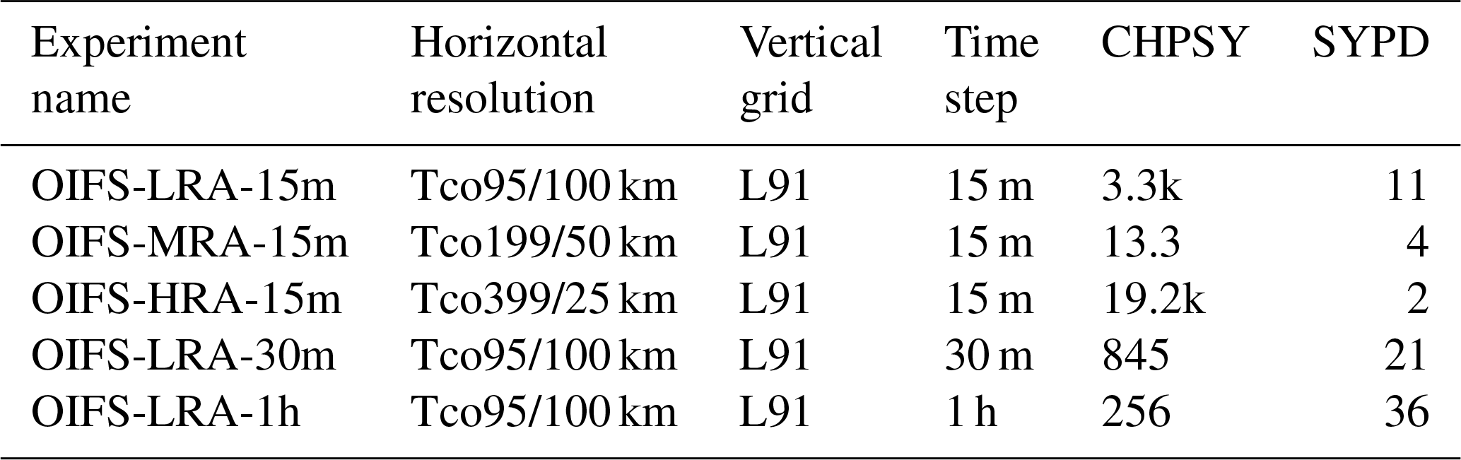
Our study is partly motivated by evaluating the suitability of various OpenIFS configurations for coupled climate simulations with FOCI-OpenIFS (Kjellsson et al., 2020) with an atmosphere horizontal resolution higher than that of ECHAM6 Tq63/N48 (∼200 km) in FOCI (Matthes et al., 2020). Our choices thus fall on three different horizontal resolutions: a low resolution (Tco95, ∼100 km), a medium resolution (Tco199, ∼50 km), and a high resolution (Tco399, ∼25 km). The Tco95 grid is the lowest acceptable resolution since the supported lower-resolution grids, e.g. Tl95/N48 and Tq42/F32, are either similar to Tq63 in ECHAM6 or coarser. The Tco399 grid was chosen as an upper limit of what is computationally feasible for AMIP integrations and century-long coupled integrations given our computer resources. All the configurations share the same vertical L91 grid. We did not modify any other model parameters when changing the model horizontal resolutions or model time steps, but we note that some parameters such as launch momentum flux for non-orographic gravity waves scale with resolution in the model. We performed five experiments in total (Table 1). For simplicity, we now refer to OpenIFS as OIFS in the rest of the sections. We note that exploring the effect of different time steps was only done for the lowest horizontal resolution (Tco95, ∼100 km). We did not run similar sensitivity experiments for the high-resolution configuration (Tco399, ∼25 km) for two reasons. First, the high-resolution configuration is very computationally expensive. Second, it was deemed to be more important to explore time step sensitivity at a low resolution since this configuration (and other similar resolutions) is often used for coupled climate simulations. The potential time step sensitivity at a high resolution is discussed in the Discussion section.
The lower boundary conditions, i.e. SST and SIC, are taken from the Atmospheric Model Intercomparison Project (AMIP) version 1.1.6 (Eyring et al., 2016; Taylor et al., 2012); they are available as monthly means on a 1° × 1° horizontal grid. The external forcing is identical to that used in the CMIP6 AMIP simulations, except for the aerosol and ozone concentrations, which are taken from monthly mean climatologies. SST and SIC are interpolated from monthly to daily frequency and from 1° × 1° horizontal resolution to the OIFS horizontal grid using bilinear interpolation. All the simulations are run for the period 1979–2019. We extend the simulations beyond the AMIP protocol for 1979–2014 up to 2019 by using SST and SIC from the ERA5 reanalysis and the Shared Socioeconomic Pathway 5 (SSP5-8.5) emission scenario. Ozone concentrations are taken from monthly photochemical equilibrium states, and aerosol concentrations are taken from monthly CAMS climatologies of 11 species.
The amplitude and phase speed of Rossby waves were computed by performing a Fourier decomposition analysis on 300 hPa daily meridional winds. First, we interpolated both ERA5 and OIFS simulation datasets onto a 2.5° × 2.5° grid using bilinear interpolation. We then applied the Fourier decomposition analysis to determine the amplitude and position for each Rossby wave number at each latitude as a function of time. Phase speed is computed as the difference in the daily position of each wave and stored at the midpoints in the time dimension. For consistency, wave amplitudes are interpolated to the midpoints in time as well. Lastly, seasonal averages are computed from the daily data for the boreal and austral winter seasons over the time period 1979–2019. In the case of phase speed, it is weighed by the corresponding daily (midpoint) amplitude squared when computing the seasonal averages in order to account for the impact of higher-amplitude events. The results are presented in wavenumber–latitude diagrams, similarly to previous studies (e.g. Pilch Kedzierski et al., 2020; Wolf and Wirth, 2017). Our wavenumber–latitude analysis is not directly comparable to either of the studies mentioned above because we did not apply any high-pass filtering in time before the Fourier decomposition. While the previous literature had similar diagrams with varying measures of wave amplitude, our detailed analysis of phase speed in such a manner is novel in the literature, to our knowledge, and is a strong addition as a model performance diagnostic.
The weather regime patterns (WRPs) were calculated using daily 500 hPa geopotential height (Z500) anomalies over the Euro–Atlantic region (30–90° N, 80° W–40° E) for the boreal winter season during the period 1979–2019. The daily Z500 anomalies were computed by subtracting the daily climatology smoothed by a 20 d running mean from the raw Z500 data. We calculated the first four empirical orthogonal functions (EOFs) from the ERA5 dataset. In the next step, the OIFS-simulated Z500 anomalies were projected onto the ERA5 EOFs to obtain pseudo principal components (pseudo-PCs). We then applied a K-means clustering algorithm to the individual model pseudo-PCs and observation PCs using four clusters. We chose four clusters because these give the most of the significant clustering. Spatial WRPs are obtained by compositing over all daily Z500 anomalies for each regime. More information about the methodology can be found in Fabiano et al. (2020), Sect. 3.1. In order to evaluate the WRPs simulated by the OIFS across configurations more quantitatively, we have additionally estimated the Pearson's pattern correlation coefficient (PCC) between the WRPs identified in the model and ERA5.
We compare the climate of OIFS to observational and reanalysis datasets. Precipitation is validated against the Global Precipitation Climatology Project (GPCP; Huffman et al., 1997), and the surface air temperature (SAT) is validated against the CRUTEM4 (Harris et al., 2014; Osborn and Jones, 2014). We have used the ERA5 reanalysis (Hersbach et al., 2020) to evaluate 10 m surface wind and the zonal wind at 300 hPa for the Rossby wave analysis. We use Z500 from ERA5 to validate the OIFS-simulated weather regimes. We also compare our results with the MERRA2 reanalysis (Gelaro et al., 2017) and find similar results. Therefore, the comparison with MERRA2 is not shown. The bootstrapping (in total 2000 iterations) method is used to compute the 95 % confidence interval for the RMSE and the WRP correlation.
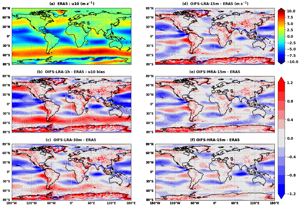
Figure 1(a) Annual mean ERA5 surface zonal wind [m s−1]. (b–d) Annual mean zonal wind [m s−1] bias for different model time steps (1 h (b), 30 m (c), and 15 m (d)) using ∼100 km resolution and (e, f) with different horizontal resolutions (∼50 (e) and ∼25 km (f)). Biases are computed with respect to ERA5 over the period 1979–2019.
3.1 Global and regional surface bias and deriving processes
The annual mean 10 m zonal wind (surface wind hereafter) bias during the period 1979–2019 for the different OIFS configurations is shown in Fig. 1. We find that the OIFS-LRA-1h configuration has a large surface wind bias over most of the world ocean, with positive biases in the mid-latitudes (the Southern Ocean, North Atlantic, and North Pacific) and negative surface wind biases over the tropical oceans (tropical Pacific, tropical Indian, and Atlantic Ocean) (Fig. 1b). Thus, the OIFS-LRA-1h configuration simulates too-strong surface westerly winds (and wind speed) over the mid-latitude oceans, which, if coupled to an ocean model, may cause biases in upper-ocean mixing and oceanic uptake of heat and carbon.
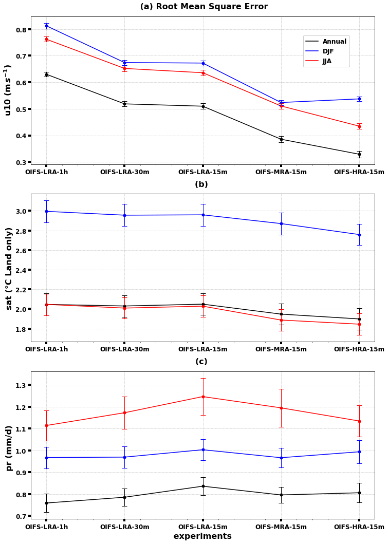
Figure 2Root mean squared error of surface zonal wind (a), SAT (b), and precipitation (c) over the period 1979–2019 for all the configurations: annual (black) and seasonal mean (DJF: blue, JJA: red). The error bars represent a 95 % confidence interval.
The surface wind bias in the OIFS-HRA-15m configuration is reduced significantly (Fig. 1f) over most of the world ocean compared to the OIFS-LRA-1h configuration (Fig. 1b), indicating that increasing the horizontal resolution from 100 to 25 km and shortening the time step from 1 h to 15 min improves the representation of the surface winds. The surface wind bias is also significantly reduced everywhere in the OIFS-MRA-15m configuration (Fig. 1e) compared to the OIFS-LRA-1h configuration (Fig. 1b). The surface wind bias in OIFS-MRA-15m is larger than that in the OIFS-HRA-15m configuration but smaller than that in the OIFS-LRA-1h configuration. Similar conclusions are obtained by performing root mean square error (RMSE) analysis, which shows that the OIFS-HRA-15m configuration has the lowest annual and global mean RMSE of surface wind, while the OIFS-LRA-1h configuration has the highest RMSE (Fig. 2a, black line). Though we have found a significant improvement in the wind bias in the OIFA-HRA-15m configuration, it is not clear yet whether the improvement is due to the increased horizontal resolution or the shorter time step.
Surface wind bias is also reduced in both the OIFS-LRA-30m (Fig. 1c) and OIFS-LRA-15m (Fig. 1d) configurations compared to the OIFS-LRA-1h configuration (Fig. 1b), and the bias improvement is mostly observed at the same places as in the OIFS-HRA-15m configuration (Fig. 1f). The surface wind bias improvement is similar in the OIFS-LRA-30m and OIFS-LRA-15 configurations, except over the North Pacific and Southern Ocean, where the OIFS-LRA-15m configuration has a smaller wind bias than the OIFS-LRA-30m configuration. However, we have not seen a large difference between the OIFS-LRA-30m and OIFS-LRA-15 configurations in the global average RMSE analysis (Fig. 2a).
The surface wind bias improvement in the OIFS-HRA-15m and OIFS-LRA-15m configurations not only exists in the annual average but also in boreal winter (DJF) and summer (JJA) (Fig. 2a blue and red lines, respectively). Our results are consistent with Jung et al. (2012) as they found a reduction in wind bias in the tropical Pacific region when they shortened the time step in their coarse-resolution configuration. However, this study and the Jung et al. (2012) study are not consistent with that of Roberts et al. (2018), who did not find much time step sensitivity. We speculate that, in Roberts et al. (2018), the reduction from 20 to 15 min in their high horizontal resolution (25 km) may be too small. Alternatively, the 20 min time step could be the optimal time step for the 25 km configuration.
The surface wind biases in the OIFS-HRA-15m and OIFS-LRA-15m configurations look similar in pattern, but they differ in magnitude. The OIFS-HRA-15m configuration has a smaller bias in the North Pacific, Peru upwelling, and Agulhas Bank regions compared to the OIFS-LRA-15m configuration. We hypothesize that the reduction in surface wind bias in the OIFS-HRA-15m configuration (Fig. 1f) compared to the OIFS-LRA-1h configuration (Fig. 1b) is a combination of the enhanced horizontal resolution and shorter time step. The improvement in the OIFS-HRA-15m configuration (Fig. 1f) compared to the OIFS-LRA-15m configuration (Fig. 1d) is due only to the enhanced horizontal resolution as both configurations use the same time step.
The zonal wind bias improvement in the OIFS-LRA-15m is further explored using the online zonal wind tendencies from OIFS, which are split into dynamics and physics that include turbulent diffusion, gravity wave drag, and convection:
where is the sum of the tendencies from advection, pressure gradient, and Coriolis force; includes tendencies from surface processes, vertical diffusion, and orography drag; includes gravity wave drag and non-orographic drag; and is the tendency from convection. The individual tendencies on the right-hand side of Eq. (1) are referred to as Dyn, Turb, Gwd, and Conv, respectively. They were stored for each model level in the OIFS-LRA-1h and OIFS-LRA-15m configurations. The lowest model level is at 10 m height (assuming surface pressure of 1013 hPa), so the 10 m wind will behave very similarly to the wind at level k=91.
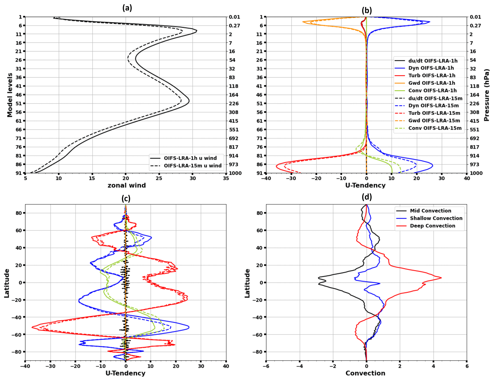
Figure 3(a) Averaged zonal wind (u) [m s−1] and (b) zonal wind tendencies [m s−2 h−1] over the Southern Ocean (40–60° S, all longitudes) as a function of height for OIFS-LRA-1h and OIFS-LRA-15m. Model levels (y axis left) and pressure levels (y axis right). (c) Zonal and time average of zonal wind tendencies at the lowest level of the model as a function of latitude. (d) Zonal and time average convection difference [Kg m−2 h−1] between the OIFS-LRA-15m and OIFS-LRA-1h configurations. The solid lines in panels (b) and (c) show the wind tendency for the OIFS-LRA-1h configuration, whereas the dashed lines are for the OIFS-LRA-15m configuration. Shown are averages over 1979–2019.
The averaged zonal wind and zonal wind tendencies over the Southern Ocean (40–60° S and all longitudes) in the OIFS-LRA-1h and OIFS-LRA-15m configurations are shown in Fig. 3a and b, respectively. The zonal wind tendency (i.e. ) in both the OIFS-LRA-15m and OIFS-LRA-1h configurations is very small ( to 0.04 m s−1) compared to the other processes (Fig. 3b, black lines). Conv provides westward acceleration between the 700 and 900 hPa pressure levels and eastward acceleration below, indicating a downward transport of westward momentum. Dyn acts to accelerate the flow eastward from 700 hPa and below, likely via momentum advection, pressure gradient, and Coriolis forces, while Turb has the opposite effect, likely via surface friction and vertical mixing processes. In the OIFS-LRA-15m configuration, we find a similar balance as in the OIFS-LRA-1h, but the westward acceleration above and eastward acceleration below are enhanced by Conv, likely by increased downward momentum transport, in agreement with the increased shallow and mid-level convection (Fig. 3d). The vertical momentum mixing by shallow and mid-level convection reduces the vertical wind shear, making the westerly winds more barotropic. As a result, the westerly winds weaken throughout the troposphere and even in the stratosphere (Fig. 3a). We note similar changes in the Northern Hemisphere mid-latitudes, suggesting that similar mechanisms are acting here. Gwd has a negligible role in the winds in the lower stratosphere and troposphere, and the Gwd term does not appear to be sensitive to the model time step (Fig. 3b, orange lines).
Figure 3c shows the zonal average of the zonal wind tendencies at the lowest level of the model as a function of the latitude. In the OIFS-LRA-1h configuration, Conv and Dyn accelerate the surface westerly wind in the mid-latitudes (∼40 to ∼60° N) in both hemispheres, and these westerly winds are partly balanced by Turb (Fig. 3c, solid lines). Dyn makes a larger contribution to accelerating the surface westerly winds than Conv (Fig. 3c, solid lines). However, the Conv contribution is enhanced in the OIFS-LRA-15m configuration, while the Dyn contribution is reduced (Fig. 3c, dashed lines). We also find that the contribution to slowing the westerly wind is reduced by Turb in the OIFS-LRA-15m configuration (Fig. 3c, dashed lines).
It is also noteworthy that the individual wind tendencies are significantly larger in the Southern Hemisphere (and Southern Ocean) than in the Northern Hemisphere (Fig. 3c). The larger magnitudes of the tendencies over the Southern Ocean compared to similar latitudes in the Northern Hemisphere are likely due to the Southern Hemisphere having fewer continents in the mid-latitudes than the Northern Hemisphere, and, thus, the surface is less rough and allows for stronger winds. In the low latitudes, both Dyn and Conv contribute to accelerating the easterly winds, which are partly balanced by Turb in the OIFS-LRA-1h configuration (Fig. 3c, solid lines). There are no discernible changes in Conv, Dyn, or Turb from OIFS-LRA-1h to OIFS-LRA-15m, indicating that the tropical surface winds are relatively insensitive to the model time step (Fig. 3c, dashed lines).
In addition to surface wind, we also investigated the sensitivity of the model time step and horizontal resolution for SAT and precipitation. The RMSEs for SAT and precipitation are shown in Fig. 2b and c, respectively. We find that the OIFS-HRA-15m has the lowest SAT RMSE of all model experiments in terms of both annual and seasonal means, although the RMSE difference across the configurations is not significant (Fig. 2b). The reduced SAT RMSE in the OIFS-HRA-15m configuration is primarily due to the lowered SAT bias over North America and the eastern part of Russia. Compared to the OIFS-LRA-1h, the SAT RMSE decreases with increased horizontal resolution (OIFS-HRA-15m and OIFS-MRA-15m), and there is no notable improvement when shortening the time step (OIFS-LRA-30m and OIFS-LRA-15m) (Fig. 2b).
We have computed the SAT and precipitation biases with a three-point smoothing, i.e. approximately 3×3° spatial smoothing, which eliminates the wiggles near steep topography arising from the Gibbs' phenomenon in the model spectral fields. We find that smoothing the fields does not change the main result that precipitation biases increase with shorter time steps in Tco95 and then decrease somewhat with higher horizontal resolutions. Hence, the wiggles are not the main source of precipitation biases, and their presence does not impact the findings of this study.
The OIFS-LRA-1h experiment exhibits the lowest precipitation RMSE of all experiments, with RMSE increasing with a shorter time step (OIFS-LRA-15m) and increased horizontal resolution (OIFS-HRA-15m) for both the annual and boreal winter means (Fig. 2c, black and blue lines). The patterns of regional precipitation biases are similar across the configurations in the middle and high latitudes, whereas the precipitation biases increase in the tropics at the high horizontal resolution or in the smaller time step configuration (not shown). The results suggest that some of the cloud and/or convection parameters may be dependent on resolution or time step and need retuning for each configuration.
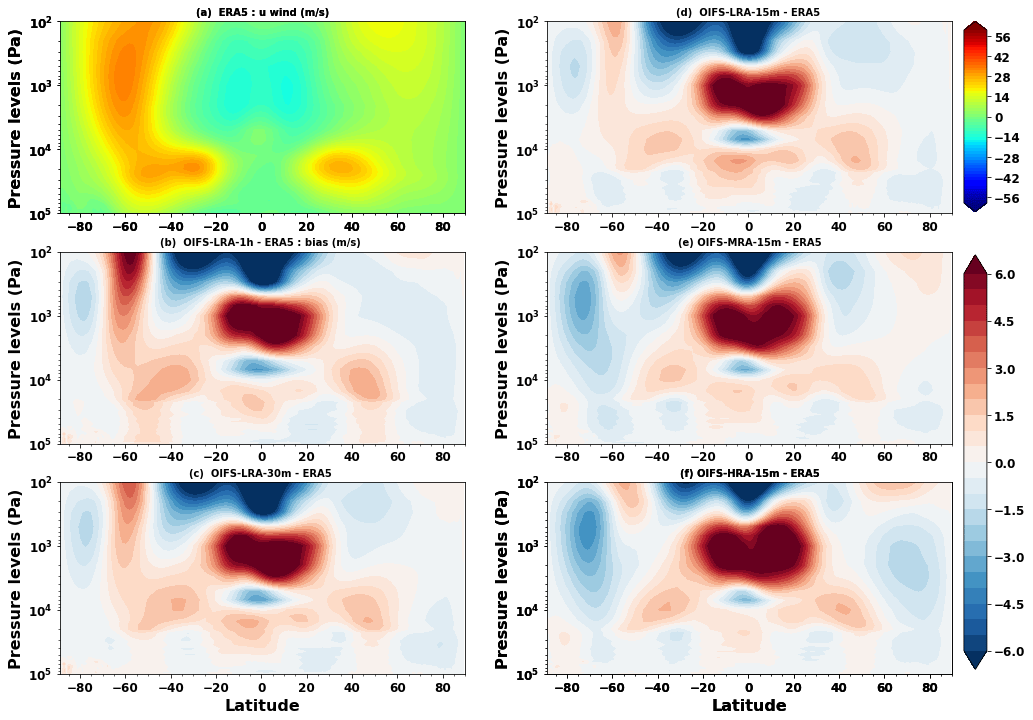
Figure 4(a) Annual zonal mean ERA5 zonal wind [m s−1]. (b, d) Annual zonal mean zonal wind [m s−1] bias for different model time steps (1 h (b), 30 m (c), and 15 m (d)) using ∼100 km resolution and (e, f) with different horizontal resolutions (∼50 (e) and ∼25 km (f)). Biases are computed with respect to ERA5 over the period 1979–2019.
3.2 Wind and temperature bias in the upper atmosphere
We examined the zonal mean u wind bias at different model levels, and it is shown in Fig. 4. We find that zonal mean u wind bias over the tropical region (40° S and 40° N) is positive and independent of model horizontal resolution and model time step (Fig. 4b–f). The OIFS-HRA-15m configuration has a relatively large negative bias in the Northern Hemisphere compared to the other configurations. The OIFS-LRA-15m and OIFS-HRA-15m zonal mean u wind biases are similar to those in Roberts et al. (2018). However, the zonal mean u wind bias in the Southern Hemisphere is not consistent across horizontal resolutions or model time steps. The zonal mean u wind bias in mid-latitudes (i.e. 70 to 50° S) is positive and large in the OIFS-LRA-1h configuration and is reduced throughout the pressure levels by shortening the model time step in the coarse-resolution OpenIFS configuration (i.e. OIFS-LRA-30m and OIFS-LRA-15m), whereas the negative zonal wind bias south of 70° S in the coarse-resolution configuration is consistent across the different time steps (Fig. 3b–d). It is also interesting to note that both OIFS-MRA-15m and OIFS-HRA-15m configurations exhibit a negative bias over the Southern Ocean (SO) at most of the pressure levels, which is not seen in either the standard OIFS-LRA-1h configuration or the OIFS-LRA-30m or OIFS-LRA-15m configurations. Overall, we conclude that, by reducing the model time step in the coarse-resolution configuration, we improve winds not only at the surface but also at higher model levels, mostly over the SO. A similar conclusion does not hold for the OIFS-MRA-15m and OIFS-HRA-15m configurations as both suffer from large negative biases over the SO.
We also examined the zonal mean temperature bias at different pressure levels. We find a cold bias (1.5 to 6 °C) in the troposphere and lower stratosphere and a warm bias (1.5 to 6 °C) above the stratosphere across the configurations (figure not shown). This indicates that OpenIFS simulations (independent of model time step and horizontal resolution) are colder than observations in the lower stratosphere and warmer above. The cold bias in the lower stratosphere is larger in the high resolution (i.e. OIFS-HRA-15m), and the warm bias above the stratosphere is smaller compared to the other configurations. Roberts et al. (2018) noticed a similar zonal mean temperature bias and speculated that the zonal mean temperature bias is linked with the sensitivity of spurious mixing due to convection and diffusion.
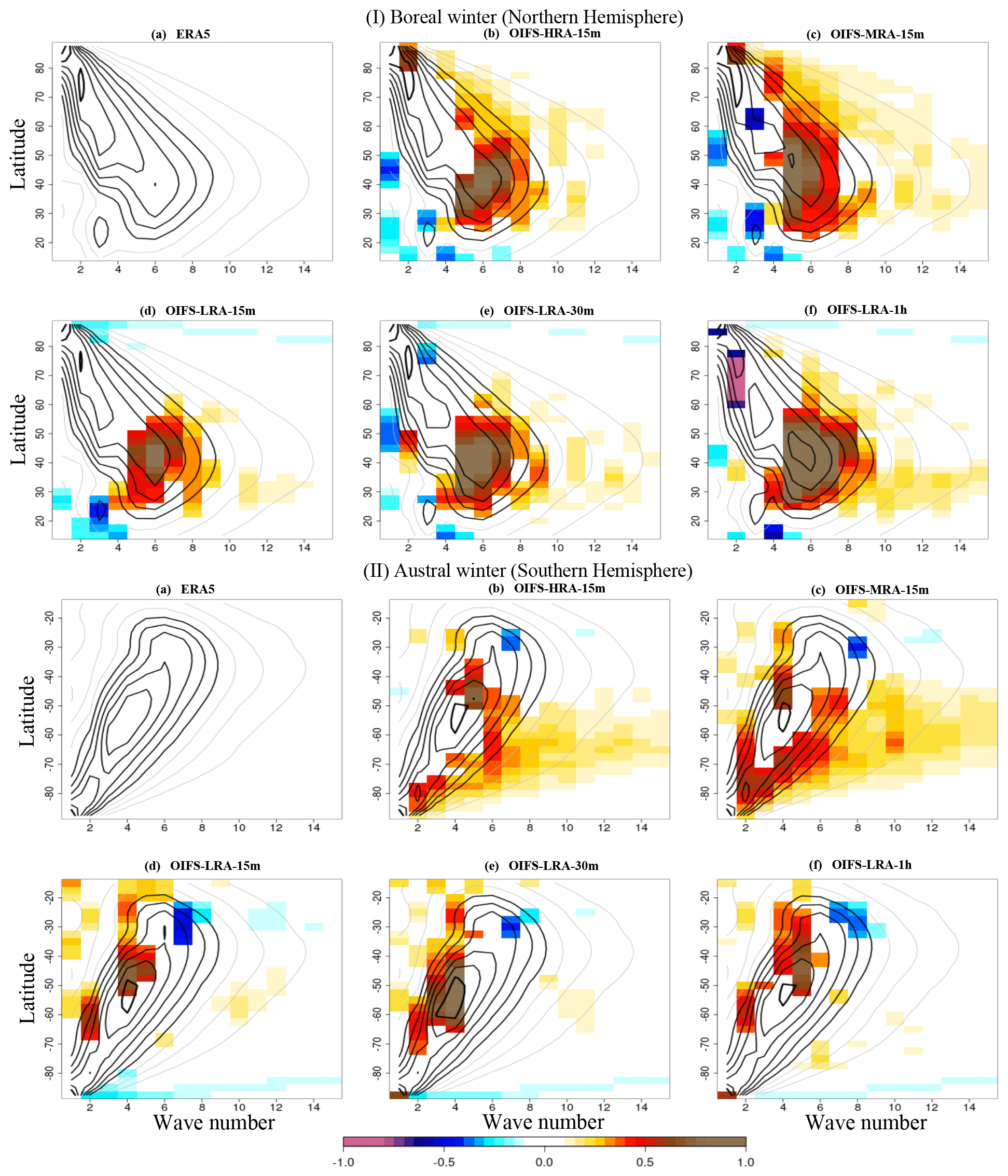
Figure 5(I) The Rossby wave amplitude (contours) for different wave numbers in the Northern Hemisphere at 300 hPa (a) in ERA5 observations and (b–f) in the OIFS model simulations during 1979–2019 in DJF (i.e. boreal winter). The colour shows the difference in wave amplitude between the model and ERA5 where it is significant at the 95 % confidence level. The wave amplitude and contour interval are shown in m s−1. The grey contours start from 2 m s−1 and the black contours from 5 m s−1, and the contour interval is 1 m s−1. (II) is similar to (I) but for JJA (i.e. austral winter).
3.3 Rossby wave analysis
Figure 5 shows the Rossby wave amplitude (grey and black contours) for ERA5 and the individual OIFS simulations for the boreal winter (Fig. 5I, DJF, Northern Hemisphere (NH)) and austral winter (Fig. 5II, JJA, Southern Hemisphere (SH)). The colour in Fig. 5 denotes the wave amplitude bias relative to ERA5 (model – ERA5). We focus only on those wave numbers and latitudes that have the highest wave amplitude because these waves explain most of the variability. The region where the wave amplitude is larger than 5 m s−1 is termed the “core region”, which mostly covers the area that is occupied by the thick black contours in Fig. 5. In DJF (NH), north of 70° N, the Rossby wave numbers k=1 and k=2 have the largest amplitudes in ERA5, whereas at the mid-latitudes (30 to 60° N), the wave numbers between about k=3 and k=9 have large amplitudes, with the largest amplitude amounting to 8 m s−1 at about 40° N for the wave number k=6 (Fig. 5Ia). During JJA (SH), the wave amplitude is located in a similar core region (Fig. 5IIa) as that in DJF (NH). The amplitude is largest south of 70° S for the wave numbers k=1 and k=2, whereas at the mid-latitudes (45 to 65° S), the wave numbers between about k=3 to k=5 have large amplitudes, with the largest amplitude amounting to 9 m s−1 being found at 57.5° S for the wave number k=4 (Fig. 5IIa).
In DJF (NH), the OIFS-LRA-1h configuration exhibits a positive bias of ∼1 m s−1 in Rossby wave amplitude (i.e. the wave amplitude bias in OIFS-LRA-1h is larger than the ERA-5) in the core region, in particular for wave numbers k=3–8 at latitudes between 25 to 55° N, and a negative bias at latitudes between 60 to 80° N for wave number k=2 (Fig. 5If). The wave amplitude biases around the core region in OIFS-LRA-1h in the mid-latitudes (20 to 40° N) are small (∼0.2) for the higher wave numbers and get better with a shorter time step configuration (OIFS-LRA-15m).
The Rossby wave amplitude biases in the OIFS-HRA-15m configuration are strongly reduced compared to the OIFS-LRA-1h configuration over the core region (Fig. 5Ib and If). The Rossby wave amplitude bias reduction in the OIFS-MRA-15m configuration is mostly similar to that in the OIFS-HRA-15m configuration, except for the wave number k=7 at 45° N, where the wave amplitude bias is larger in the OIFS-HRA-15m configuration (Fig. 5Ib and Ic). The OIFS-HRA-15m and OIFS-MRA-15m configurations also exhibit a positive bias for wave number k=2 at high-latitudes of 60 to 80° N. The OIFS-MRA-15m configuration also shows a negative bias for the wave number k=3 at latitudes between 60 to 65° N in the core region, which is not present in the other configurations. The OIFS-HRA-15m and OIFS-MRA-15m configurations show similar biases around the core region as in the OIFS-LRA-1h configuration; i.e. high-resolution and OIFS-LRA-1h configurations overestimate wave amplitudes for the higher wave numbers. The Rossby wave amplitude biases are progressively reduced from the OIFS-LRA-1h configuration to the OIFS-LRA-30m and OIFS-LRA-15m configurations (Fig. 5Id–If), indicating a sensitivity of model bias to the time step. The wave amplitude bias for wave number k=7 at 45° N exists in all the configurations, and it is smaller in the OIFS-LRA-15m and OIFS-MRA-15m configurations than in the other configurations. Overall, both the OIFS-LRA-15m and OIFS-HRA-15m configurations are able to reproduce the observed Rossby wave amplitudes in DJF (NH) better than OIFS-LRA-1h.
In JJA (SH), the Rossby wave amplitude bias in the core region is smaller than in DJF (NH) for all the configurations (Fig. 5I and II). OIFS-LRA-1h exhibits a positive bias of ∼0.5 m s−1 in JJA (SH) for the wave number k=2 at latitudes between ∼50 and ∼62.5° S and for wave numbers k=4 to k=5 between 30 and 40° S (Fig. 5IIf). The OIFS-LRA-30m configuration shows a positive bias for the wave numbers k=2 to k=5 at latitudes between 40 and 70° S, which is larger than other configurations.
The OIFS-HRA-15m and OIFS-MRA-15m configurations exhibit a positive bias ∼0.5 m s−1 around the core region and at latitudes of 50 to 70° S; this bias does not exist in the other coarse-resolution configurations (Fig. 5IIb–IIf). The Rossby wave amplitude biases around the core region at the mid-latitudes in the high-resolution simulations are consistent and larger in the SH than in the NH (Fig. 5Ib, c and IIb, c).
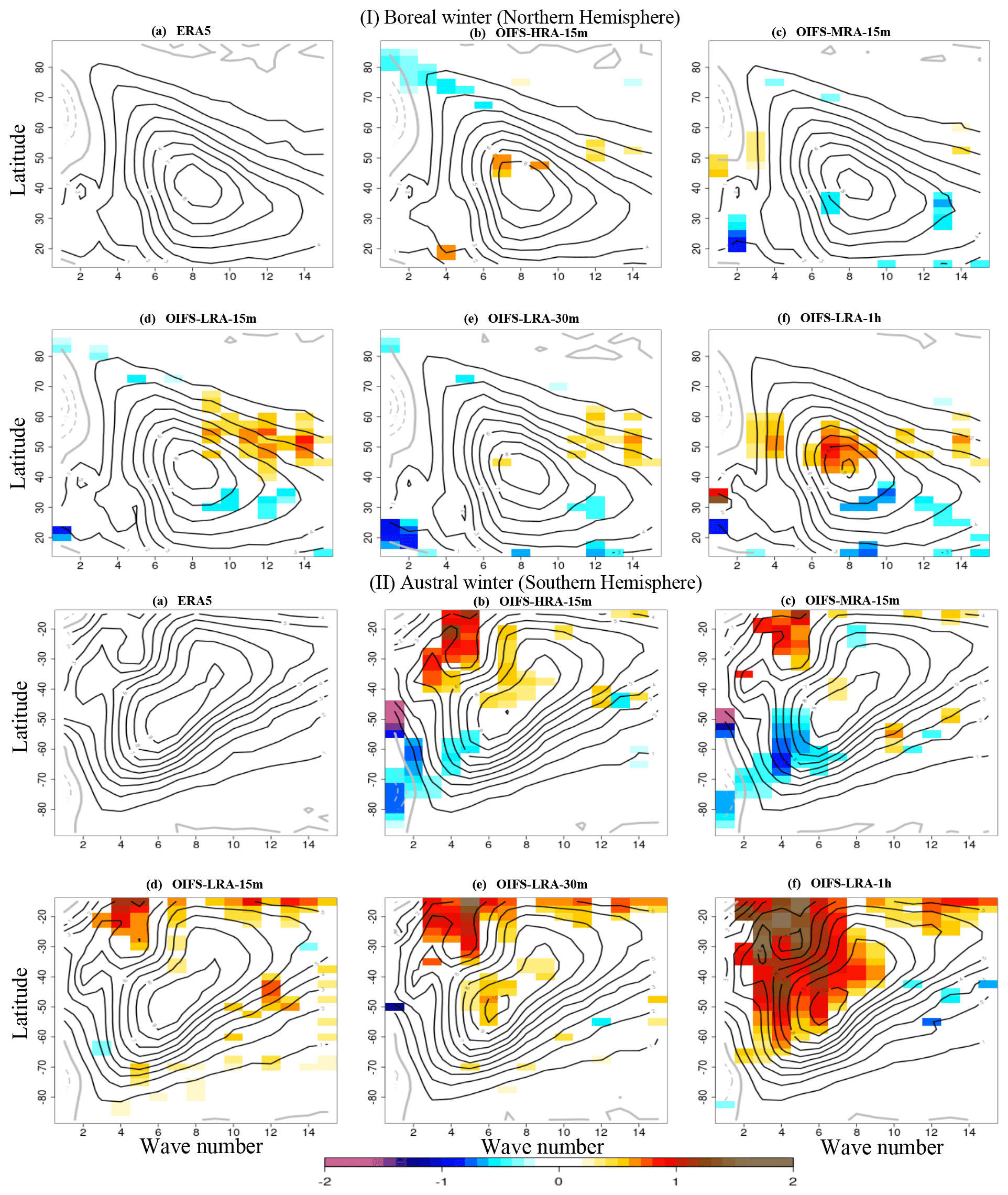
Figure 6(I) The Rossby wave phase speed (contours) for different wave numbers at 300 hPa in the Northern Hemisphere (a) in ERA5 observations and (b–f) in the OIFS model simulations during 1979–2019 in DJF (i.e. boreal winter). The colour shows the differences in wave phase speed between model and ERA5, where it is significant at the 95 % confidence level. The wave phase speed and contour interval are shown in m s−1. The black contours start from 1 m s−1, and the contour interval is 1 m s−1. Panel (II) is similar to panel (I) but for JJA (i.e. austral winter). The dashed contours show a negative phase speed, and a grey contour shows zero phase speed.
We also analyse the phase speed of Rossby waves for ERA5 and across the OIFS's configurations for DJF (NH) and JJA (SH) seasons (Fig. 6). In the ERA5 dataset (Fig. 6Ia), the Rossby wave phase speed is positive (i.e. eastward moving, solid contour) for wave numbers greater than 2 (i.e. k>2) at most latitudes. The wave numbers k=1 to k=2 have a positive wave phase speed from the Equator to 55° N and a negative wave phase speed (i.e. westward moving, dashed contours) between 60 and 80° N in DJF (NH) (Fig. 6Ia). The maximum phase speed is found at wave number k=8 at 40° N, while the minimum is found at wave number k=1 at 60° N (Fig. 6Ia). In JJA (SH) (Fig. 6IIa), the wave phase speeds are mostly positive and large for all the wave numbers and at each latitude, with the maximum phase speed being observed for the wave numbers between k=6 and k=8 and latitudes between 40 and 60° S, and these waves move faster than those in DJF (NH).
The OIFS-LRA-1h configuration suffers from positive phase speed biases for wave numbers k=4 to k=8 at latitudes between 42.5 and 60° N; i.e. waves move faster eastward than in ERA5, and the bias is larger than 1 m s−1. The bias of ∼1 m s−1 for wave numbers k=6 to k=8 at 40 and 60° N is of particular concern as it is near the maximum wave amplitudes in DJF (Fig. 6If). In general, phase speed biases in the OIFS-LRA-1h configuration are strongly reduced as either the horizontal resolution is increased or the time step is shortened (Fig. 6Ib–If). In JJA (SH), the OIFS-LRA-1h configuration exhibits a very large (between ∼1.5–2 m s−1) Rossby wave phase speed bias for most of the wave numbers, which is largest for the wave numbers k=2 to k=8 between 15 to 55° S (Fig. 6IIf). Large biases can be found between 15 and 25° S (∼1.5 m s−1) for most of the wave numbers, but the wave activity is low there (Fig. 6IIf). The large phase speed biases are strongly reduced in the OIFS-LRA-30m and OIFS-LRA-15m configurations (Fig. 6IId–IIf), indicating a strong sensitivity to the reduced biases in mean winds and wind speeds (Fig. 1). Overall, the Rossby wave speed bias in the OIFS-HRA-15m configuration is smaller than in the OIFS-LRA-1h configuration (Fig. 6IIb and IIf). However, we note that both the OIFS-MRA-15m and OIFS-HRA-15m configurations exhibit negative biases south of 55° S for wave numbers k=1 to k=5; that is, the eastward-moving waves are slower than in ERA5 (Fig. 6IIb).
The wave phase speed analysis reveals a clear improvement in the representation of the Rossby waves in the boreal winter (i.e. NH) when increasing the horizontal resolution and shortening the model time step compared to the OIFS-LRA-1h configuration. In austral winter, however, the representations of Rossby wave amplitudes and phase speeds are the most realistic in the OIFS-LRA-15m configuration, with longer time steps introducing too-fast phase speeds and higher horizontal resolutions introducing too-slow phase speeds at wave numbers less than 6 (i.e. k<6).
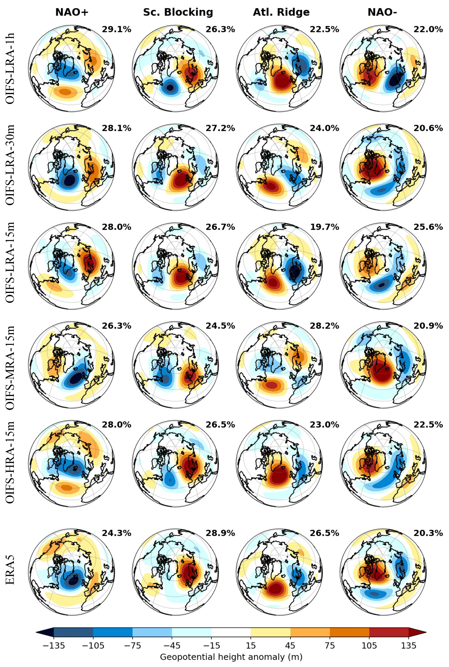
Figure 7Weather regime patterns over the Euro–Atlantic regions from ERA5 observation (bottom row) and the individual OIFS model simulations (first to fifth row) over the time period 1979–2019 for DJF (boreal winter season).
3.4 Weather regime pattern
We derive the four weather regimes patterns (WRPs) over the NH in the Euro–Atlantic region from ERA5. The patterns resemble the positive and negative phases of the North Atlantic Oscillation (NAO+ and NAO−, respectively), the Scandinavian blocking (Sc. Blocking) pattern, and the North Atlantic ridge (Atl. Ridge) pattern (Fig. 7, bottom row). These WRPs are consistent with the previous findings (Dawson et al., 2012; Fabiano et al., 2020, 2021).
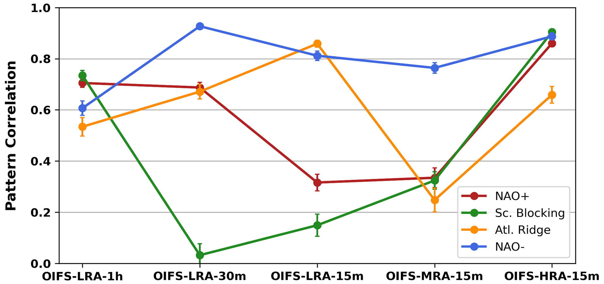
Figure 8Pattern correlation coefficient of the individual weather regimes between OIFS model configurations and ERA5 for the period 1979–2019 for the DJF season. The error bars represent a 95 % confidence interval.
The OIFS-HRA-15m configuration produces WRPs that are more visually similar to those in ERA-5 than OIFS-LRA-1h does (Fig. 7), a result confirmed by the higher pattern correlation coefficient (PCC) between OIFS-HRA-15m and ERA5 compared to that between OIFS-LRA-1h and ERA-5 (Figs. 7 and 8). The PCCs for NAO+, NAO−, and Sc. Blocking all exceed 0.8 in OIFS-HRA-15m, while OIFS-LRA-1h does not achieve PCCs above 0.8 for any WRP (Fig. 8).
The OIFS-MRA-15m configuration shows smaller PCCs than both the OIFS-HRA-15m and OIFS-LRA-1h configurations (Fig. 8); i.e. the improvement from OIFS-LRA-1h to OIFS-HRA-15m does not have a linear relationship with model horizontal resolution or time step. Compared to other configurations and ERA5, the OIFS-MRA-15m Z500 anomaly in the NAO+ pattern is too elongated in the southwest–northeast direction, and an unrealistic negative Z500 anomaly over the North Atlantic appears in the Sc. Blocking regime (Fig. 7). Furthermore, OIFS-MRA-15m shows an Atl. Ridge pattern with neither the right structure nor amplitude.
There is an improvement in the representation of the NAO− regime in the OIFS-LRA-30m configuration over the OIFS-LRA-1h configuration (Fig. 7), while the Sc. Blocking regime becomes worse due to the ridge shifting westward. These changes are also reflected in the PCCs (Fig. 8). Similarly, the OIFS-LRA-15m better represents NAO− and Atl. Ridge than OIFS-LRA-1h, while NAO+ and Sc. Blocking worsened. The westward shift of the Sc. Blocking is similar in OIFS-LRA-15m and OIFS-LRA-30m, and the worse NAO+ is related to a northward shift of both the positive and negative Z500 anomalies. We note that all experiments use the same SST and sea ice conditions and that OIFS-LRA-1h, OIFS-LRA-30m and OIFS-LRA-15m share the same horizontal resolution; i.e. the changes from OIFS-LRA-1h to OIFS-LRA-15m are not due to SST biases or representation of orography. There does not seem to be a clear improvement when the time step is shortened despite the reduction in mean state biases and Rossby wave amplitudes and phase speeds.
The PCC is greater than 0.8 for three out of four WRPs in the OIFS-HRA-15m configuration; hence, we argue that the OIFS-HRA-15m has the most realistic representation of the weather regime patterns out of all experiments here. Large improvement in OIFS-HRA-15m over the other configurations could be due to better-resolved topography and land–sea contrasts.
We have investigated the sensitivity of the climate biases in the OpenIFS atmosphere model to changes in horizontal resolution and time step by analysing AMIP simulations for the period 1979–2019 (Table 1). The strong positive surface zonal wind bias over the Southern Ocean and Northern Hemisphere mid-latitudes and the negative bias in the tropical and subtropical regions were significantly improved in the high-horizontal resolution configuration with a short time step (∼25 km, OIFS-HRA-15m). A similar improvement is observed in the coarse-horizontal-resolution version with a shorter time step (∼100 km with 30 or 15 min). The zonal wind bias over the mid-latitudes in both hemispheres is reduced throughout the air column when a smaller time step is used in the coarse-resolution version, and we find that the changes in the surface winds are largely due to enhanced shallow and mid-level convection, which increases vertical momentum transport. Biases in the surface westerlies in mid-latitudes are common in CMIP-class climate models (Bracegirdle et al., 2020), and a sensitivity to friction has been noted in idealized model studies (Chen and Plumb, 2009). We hypothesize that the enhanced shallow and mid-level convection with a shorter model time step and/or increased horizontal resolution deepened the layer over which friction acts in the lower troposphere so that the frictional effects on the barotropic jet increased, leading to a poleward shift in the jet and reduced biases in zonal wind.
We also find a notable improvement in the representation of the Rossby wave amplitude and phase speed with increased horizontal resolution and shorter time steps, at least for the waves accounting for the most variability in both austral and boreal winter seasons. The reduced zonal wind throughout the troposphere with a shorter time step (Fig. 3) would decrease the eastward phase speed of Rossby waves, which may explain part of the reduced phase speeds (Fig. 6) and reduced biases. However, changes in air–sea interactions or eddy–mean flow interactions may also play a role. In particular, we note that a very large reduction in phase speed biases in austral winter in OIFS-LRA-15m compared to OIFS-LRA-1h were concurrent with very large reductions in zonal surface wind biases.
The weather regime patterns are also more realistic in the high-horizontal-resolution and short-time-step configuration OIFS-HRA-15m than in OIFS-LRA-1h, but we note that there is no consistent improvement from OIFS-LRA-1h to OIFS-HRA-15m when either the horizontal resolution is increased or the time step is shortened. For example, both OIFS-MRA-15m and OIFS-LRA-15m are worse than OIFS-LRA-1h. The improvements in the weather regime patterns and Rossby wave amplitude and speed could very well be related to each other as e.g. variations in Rossby wave breaking have been linked to the onset of NAO phases (Strong and Magnusdottir, 2008), but this would require further and more targeted analysis. The overall good representation of weather regimes in OIFS-LRA-1h compared to simulations with shorter time steps (OIFS-LRA-30m, OIFS-LRA-15m) may be due to compensation for errors. For example, it is possible that improving the wave amplitudes and phase speeds in OIFS-LRA-30m compared to OIFS-LRA-1h exposes the effect of biases caused by the coarse resolutions in both configurations, e.g. weak interactions with topography, leading to an overall worse representation of weather regimes.
We found a gradual reduction in SAT biases in OpenIFS with increased resolution or shorter time steps. The improvements were largely driven by improvements over North America and eastern Russia. Roberts et al. (2018) noted similar SAT biases and linked them to surface albedo, which is thus likely the cause here as well. The improvement with increased resolution and/or shorter time steps may be a result of improved snow cover. Systematic improvements in the precipitation biases were not observed. Instead, precipitation biases generally increased with finer horizontal resolutions or shorter time steps, suggesting that some tuning may be required in the physics parameters when changing horizontal resolutions and time steps.
We stress that the results presented in this study are specific to the OpenIFS atmosphere model and are crucial for the modelling community that uses the OpenIFS in their climate models, such as in EC-Earth (Haarsma et al., 2020; Döscher et al., 2022), CNRM (Voldoire et al., 2019), AWI (Streffing et al., 2022), and GEOMAR (Kjellsson et al., 2020). However, the results may also have implications for other climate modelling communities, at least for those that use a semi-Lagrangian scheme similar to the IFS (e.g. Walters et al., 2019) in the atmospheric component, where long time steps are both possible and often desirable to reduce the computational cost of the model.
The zonal wind bias improvement in the OpenIFS is important for research questions linked with the Southern Ocean dynamics that play a crucial role in both the global atmosphere and ocean circulation. We propose that the model time step not be longer than 30 min at any horizontal resolution to minimize surface wind biases over the ocean. The computational cost increases linearly with dt (time step), whereas the cost scales with horizontal resolution as dx^3 as the number of grid points increases in both dimensions, and the time step is likely shortened as well. Hence, reducing the model time step from 45 or 60 min to 20 or 30 min may double the computational cost but would lead to significant improvements in the simulated climate. The optimal model time step for the OpenIFS coarse-resolution model (1°) is suggested to be 30 min but should likely be somewhat shorter, e.g. 15 min, for higher resolutions. In this study, we have not investigated the sensitivity of extreme events to the model time step as our focus is mostly on mean state biases. The effect of model horizontal resolution and time step on precipitation extremes is the topic of another paper currently in preparation.
Another limitation of this study is that the time step sensitivity was only tested for the low-resolution configuration, OIFS-LRA, and not the higher resolutions, e.g. OIFS-HRA. We found that many of the surface wind biases were alleviated by a shorter time step due to increased shallow and mid-level convection (Fig. 3). We therefore speculate that a similar sensitivity should be present at a high horizontal resolution (∼25 km); i.e. a simulation with OIFS-HRA using a 1 h time step would most likely exhibit a much larger surface wind bias than the OIFS-HRA simulation with a 15 min time step.
The OpenIFS model requires a software licence agreement with ECMWF, and OpenIFS's licence is easily given free of charge to any academic or research institute. The details of the different versions of the OpenIFS model, including the OpenIFS version used in this study, i.e. 43r3, can be found at https://confluence.ecmwf.int/display/OIFS/About+OpenIFS (ECMWF, 2018). The OpenIFS model source code has been made available for the editor and reviewers.
The input datasets (both initial and boundary conditions) needed to run the OpenIFS model, the run scripts, the model output, and the Jupiter notebook that support the findings of this study are available at https://hdl.handle.net/20.500.12085/c74887dc-e609-4392-9faf-48c67276d5d1 (Savita, 2023a). The source code for XIOS 2.5, revision 1910, is available from the official repository at https://doi.org/10.5281/zenodo.4905652 (Meurdesoif, 2017) under the CeCILL_V2 licence. OpenIFS experiments were made using ESM-Tools (https://doi.org/10.5281/zenodo.5787476, Miguel et al., 2021). The OASIS coupler is available at https://oasis.cerfacs.fr/en/ (CERFACS, 2024). The XIOS, ESM-Tools, and OASIS coupler used in this study can be downloaded from https://doi.org/10.5281/zenodo.8189718 (Savita, 2023b).
The observational datasets used to validate OpenIFS model results in this study are downloadable from the ERA5 (https://cds.climate.copernicus.eu/, Hersbach et al., 2020), GPCP (https://psl.noaa.gov/data/gridded/data.gpcp.html, Huffman et al., 1997), and CRUTEM4 (http://badc.nerc.ac.uk/data/cru/, Osborn and Jones, 2014) websites. Total model output exceeds 10 Tb and is not publicly available but is available from the authors upon reasonable requests.
All the model simulations were conducted by AS and JK. Analysis of the output and the writing of the text for this paper were coordinated by AS with substantial contributions from JK, RPK, ML, TR, SW, and WP.
The contact author has declared that none of the authors has any competing interests.
Publisher's note: Copernicus Publications remains neutral with regard to jurisdictional claims made in the text, published maps, institutional affiliations, or any other geographical representation in this paper. While Copernicus Publications makes every effort to include appropriate place names, the final responsibility lies with the authors.
Abhishek Savita, Joakim Kjellsson, and Mojib Latif are supported by JPI Climate/Ocean (ROADMAP project, grant no. 01LP2002C). Wonsun Park was supported by IBS (grant no. IBS-R028-D1). We wish to thank the OpenIFS team at ECMWF for the technical support. All simulations were performed on the HLRN machine under shk00018 project resources. All analyses were performed on computer clusters at GEOMAR and Kiel University Computing Center (NESH). We give thanks to Anton Beljaars for the discussion on ECMWF model physics. We also thank both reviewers and the editor for their constructive comments and suggestions during the review process.
This research has been supported by the EU's ROADMAP project (grant no. 01LP2002C).
The article processing charges for this open-access publication were covered by the GEOMAR Helmholtz Centre for Ocean Research Kiel.
This paper was edited by Sophie Valcke and reviewed by two anonymous referees.
Athanasiadis, P. J., Ogawa, F., Omrani, N.-E., Keenlyside, N., Schiemann, R., Baker, A. J., Vidale, P. L., Bellucci, A., Ruggieri, P., and Haarsma, R.: Mitigating climate biases in the midlatitude North Atlantic by increasing model resolution: SST gradients and their relation to blocking and the jet, J. Climate, 35, 3385–3406, 2022.
Bayr, T., Latif, M., Dommenget, D., Wengel, C., Harlaß, J., and Park, W.: Mean-state dependence of ENSO atmospheric feedbacks in climate models, Clim. Dynam., 50, 3171–3194, 2018.
Beljaars, A., Balsamo, G., Bechtold, P., Bozzo, A., Forbes, R., Hogan, R. J., Köhler, M., Morcrette, J.-J., Tompkins, A. M., and Viterbo, P.: The numerics of physical parametrization in the ECMWF model, Front. Earth Sci., 6, 137, https://doi.org/10.3389/feart.2018.00137, 2018.
Bracegirdle, T., Holmes, C., Hosking, J., Marshall, G., Osman, M., Patterson, M., and Rackow, T.: Improvements in circumpolar Southern Hemisphere extratropical atmospheric circulation in CMIP6 compared to CMIP5, Earth Space Sci., 7, e2019EA001065, https://doi.org/10.1029/2019EA001065, 2020.
Branković, C. and Gregory, D.: Impact of horizontal resolution on seasonal integrations, Clim. Dynam., 18, 123–143, 2001.
CERFACS: The OOASIS Coupler, CERFACS [software], https://oasis.cerfacs.fr/en/ (last access: 30 September 2021), 2024.
Chen, G. and Plumb, R. A.: Quantifying the eddy feedback and the persistence of the zonal index in an idealized atmospheric model, J. Atmos. Sci., 66, 3707–3720, 2009.
Couldrey, M. P., Gregory, J. M., Boeira Dias, F., Dobrohotoff, P., Domingues, C. M., Garuba, O., Griffies, S. M., Haak, H., Hu, A., and Ishii, M.: What causes the spread of model projections of ocean dynamic sea-level change in response to greenhouse gas forcing?, Clim. Dynam., 56, 155–187, 2021.
Dawson, A., Palmer, T., and Corti, S.: Simulating regime structures in weather and climate prediction models, Geophys. Res. Lett., 39, https://doi.org/10.1029/2012GL053284, 2012.
Döscher, R., Acosta, M., Alessandri, A., Anthoni, P., Arsouze, T., Bergman, T., Bernardello, R., Boussetta, S., Caron, L.-P., Carver, G., Castrillo, M., Catalano, F., Cvijanovic, I., Davini, P., Dekker, E., Doblas-Reyes, F. J., Docquier, D., Echevarria, P., Fladrich, U., Fuentes-Franco, R., Gröger, M., v. Hardenberg, J., Hieronymus, J., Karami, M. P., Keskinen, J.-P., Koenigk, T., Makkonen, R., Massonnet, F., Ménégoz, M., Miller, P. A., Moreno-Chamarro, E., Nieradzik, L., van Noije, T., Nolan, P., O'Donnell, D., Ollinaho, P., van den Oord, G., Ortega, P., Prims, O. T., Ramos, A., Reerink, T., Rousset, C., Ruprich-Robert, Y., Le Sager, P., Schmith, T., Schrödner, R., Serva, F., Sicardi, V., Sloth Madsen, M., Smith, B., Tian, T., Tourigny, E., Uotila, P., Vancoppenolle, M., Wang, S., Wårlind, D., Willén, U., Wyser, K., Yang, S., Yepes-Arbós, X., and Zhang, Q.: The EC-Earth3 Earth system model for the Coupled Model Intercomparison Project 6, Geosci. Model Dev., 15, 2973–3020, https://doi.org/10.5194/gmd-15-2973-2022, 2022.
ECMWF: OpenIFS programme, ECMWF [software], https://confluence.ecmwf.int/display/OIFS/About+OpenIFS (last access: 28 February 2024), 2018.
Eyring, V., Bony, S., Meehl, G. A., Senior, C. A., Stevens, B., Stouffer, R. J., and Taylor, K. E.: Overview of the Coupled Model Intercomparison Project Phase 6 (CMIP6) experimental design and organization, Geosci. Model Dev., 9, 1937–1958, https://doi.org/10.5194/gmd-9-1937-2016, 2016.
Fabiano, F., Christensen, H., Strommen, K., Athanasiadis, P., Baker, A., Schiemann, R., and Corti, S.: Euro-Atlantic weather Regimes in the PRIMAVERA coupled climate simulations: impact of resolution and mean state biases on model performance, Clim. Dynam., 54, 5031–5048, 2020.
Fabiano, F., Meccia, V. L., Davini, P., Ghinassi, P., and Corti, S.: A regime view of future atmospheric circulation changes in northern mid-latitudes, Weather Clim. Dynam., 2, 163–180, 2021.
Flato, G., Marotzke, J., Abiodun, B., Braconnot, P., Chou, S. C., Collins, W., Cox, P., Driouech, F., Emori, S., and Eyring, V.: Evaluation of climate models, in: Climate change 2013: the physical science basis. Contribution of Working Group I to the Fifth Assessment Report of the Intergovernmental Panel on Climate Change, Cambridge University Press, 741–866, 2014.
Forbes, R. and Tompkins, A.: An improved representation of cloud and precipitation, ECMWF Newsletter, 129, 13–18, 2011.
Gates, W. L., Boyle, J. S., Covey, C., Dease, C. G., Doutriaux, C. M., Drach, R. S., Fiorino, M., Gleckler, P. J., Hnilo, J. J., and Marlais, S. M.: An overview of the results of the Atmospheric Model Intercomparison Project (AMIP I), B. Am. Meteorol. Soc., 80, 29–56, 1999.
Gelaro, R., McCarty, W., Suárez, M. J., Todling, R., Molod, A., Takacs, L., Randles, C. A., Darmenov, A., Bosilovich, M. G., and Reichle, R.: The modern-era retrospective analysis for research and applications, version 2 (MERRA-2), J. Climate, 30, 5419–5454, 2017.
Haarsma, R., Acosta, M., Bakhshi, R., Bretonnière, P.-A., Caron, L.-P., Castrillo, M., Corti, S., Davini, P., Exarchou, E., Fabiano, F., Fladrich, U., Fuentes Franco, R., García-Serrano, J., von Hardenberg, J., Koenigk, T., Levine, X., Meccia, V. L., van Noije, T., van den Oord, G., Palmeiro, F. M., Rodrigo, M., Ruprich-Robert, Y., Le Sager, P., Tourigny, E., Wang, S., van Weele, M., and Wyser, K.: HighResMIP versions of EC-Earth: EC-Earth3P and EC-Earth3P-HR – description, model computational performance and basic validation, Geosci. Model Dev., 13, 3507–3527, https://doi.org/10.5194/gmd-13-3507-2020, 2020.
Harris, I., Jones, P. D., Osborn, T. J., and Lister, D. H.: Updated high-resolution grids of monthly climatic observations–the CRU TS3. 10 Dataset, Int. J. Climatol., 34, 623–642, 2014.
Hazeleger, W., Wang, X., and Severijns, C.: SS tef anescu, R Bintanja, A Sterl, Klaus Wyser, T Semmler, S Yang, B Van den Hurk, et al. Ec-earth v2. 2: description and validation of a new seamless earth system prediction model, Clim. Dynam., 39, 2611–2629, 2012.
He, C. and Zhou, T.: The two interannual variability modes of the western North Pacific subtropical high simulated by 28 CMIP5–AMIP models, Clim. Dynam., 43, 2455–2469, 2014.
Hersbach, H., Bell, B., Berrisford, P., Hirahara, S., Horányi, A., Muñoz-Sabater, J., Nicolas, J., Peubey, C., Radu, R., and Schepers, D.: The ERA5 global reanalysis, Q. J. Roy. Meteor. Soc., 146, 1999–2049, https://doi.org/10.1002/qj.3803, 2020 (data available at: https://cds.climate.copernicus.eu/, last access: 15 February 2022).
Hogan, R. J. and Bozzo, A.: A flexible and efficient radiation scheme for the ECMWF model, J. Adv. Model. Earth Sy., 10, 1990–2008, 2018.
Huffman, G. J., Adler, R. F., Arkin, P., Chang, A., Ferraro, R., Gruber, A., Janowiak, J., McNab, A., Rudolf, B., and Schneider, U.: The global precipitation climatology project (GPCP) combined precipitation dataset, B. Am. Meteorol. Soc., 78, 5–20, https://doi.org/10.1175/1520-0477(1997)078<0005:TGPCPG>2.0.CO;2, 1997 (data available at: https://psl.noaa.gov/data/gridded/data.gpcp.html, last access: 15 February 2022).
Jung, T., Miller, M., Palmer, T., Towers, P., Wedi, N., Achuthavarier, D., Adams, J., Altshuler, E., Cash, B., and Kinter Iii, J.: High-resolution global climate simulations with the ECMWF model in Project Athena: Experimental design, model climate, and seasonal forecast skill, J. Climate, 25, 3155–3172, 2012.
Kim, S. T., Cai, W., Jin, F.-F., and Yu, J.-Y.: ENSO stability in coupled climate models and its association with mean state, Clim. Dynam., 42, 3313–3321, 2014.
Kjellsson, J., Streffing, J., Carver, G., and Köhler, M.: From weather forecasting to climate modelling using OpenIFS, ECMWF Newsletter, 164, 38–41, 2020.
Liu, B., Gan, B., Cai, W., Wu, L., Geng, T., Wang, H., Wang, S., Jing, Z., and Jia, F.: Will increasing climate model resolution be beneficial for ENSO simulation?, Geophys. Res. Lett., 49, e2021GL096932, https://doi.org/10.1029/2021GL096932, 2022.
Ma, P.-L., Harrop, B. E., Larson, V. E., Neale, R. B., Gettelman, A., Morrison, H., Wang, H., Zhang, K., Klein, S. A., Zelinka, M. D., Zhang, Y., Qian, Y., Yoon, J.-H., Jones, C. R., Huang, M., Tai, S.-L., Singh, B., Bogenschutz, P. A., Zheng, X., Lin, W., Quaas, J., Chepfer, H., Brunke, M. A., Zeng, X., Mülmenstädt, J., Hagos, S., Zhang, Z., Song, H., Liu, X., Pritchard, M. S., Wan, H., Wang, J., Tang, Q., Caldwell, P. M., Fan, J., Berg, L. K., Fast, J. D., Taylor, M. A., Golaz, J.-C., Xie, S., Rasch, P. J., and Leung, L. R.: Better calibration of cloud parameterizations and subgrid effects increases the fidelity of the E3SM Atmosphere Model version 1, Geosci. Model Dev., 15, 2881–2916, https://doi.org/10.5194/gmd-15-2881-2022, 2022.
Matthes, K., Biastoch, A., Wahl, S., Harlaß, J., Martin, T., Brücher, T., Drews, A., Ehlert, D., Getzlaff, K., Krüger, F., Rath, W., Scheinert, M., Schwarzkopf, F. U., Bayr, T., Schmidt, H., and Park, W.: The Flexible Ocean and Climate Infrastructure version 1 (FOCI1): mean state and variability, Geosci. Model Dev., 13, 2533–2568, https://doi.org/10.5194/gmd-13-2533-2020, 2020.
Meehl, G. A. and Teng, H.: CMIP5 multi-model hindcasts for the mid-1970s shift and early 2000s hiatus and predictions for 2016–2035, Geophys. Res. Lett., 41, 1711–1716, 2014.
Meng, Y., Hao, Z., Feng, S., Guo, Q., and Zhang, Y.: Multivariate bias corrections of CMIP6 model simulations of compound dry and hot events across China, Environ. Res. Lett., 17, 104005, https://doi.org/10.1088/1748-9326/ac8e86, 2022.
Meurdesoif, Y.: XIOS 2.0 (Revision 1297), Zenodo [code], https://doi.org/10.5281/zenodo.4905653, 2017.
Miguel, P. G., dbarbi, Streffing, J., seb-wahl, Wieters, N., Ural, D., Kjellsson, J., Koldunov, N., ackerlar, mbutzin, Semmler, T., Hegewald, J., mwerner-awi, chrisdane, SpontEIN, a270105, christian-stepanek, and Athanase, M.: esm-tools/esm_tools: Release 6 (v6.0.0), Zenodo [code], https://doi.org/10.5281/zenodo.5787476, 2021.
Osborn, T. J. and Jones, P. D.: The CRUTEM4 land-surface air temperature data set: construction, previous versions and dissemination via Google Earth, Earth Syst. Sci. Data, 6, 61–68, https://doi.org/10.5194/essd-6-61-2014, 2014 (data available at: http://badc.nerc.ac.uk/data/cru/, last access: 15 February 2022).
Pilch Kedzierski, R., Matthes, K., and Bumke, K.: New insights into Rossby wave packet properties in the extratropical UTLS using GNSS radio occultations, Atmos. Chem. Phys., 20, 11569–11592, https://doi.org/10.5194/acp-20-11569-2020, 2020.
Roberts, C. D., Senan, R., Molteni, F., Boussetta, S., Mayer, M., and Keeley, S. P. E.: Climate model configurations of the ECMWF Integrated Forecasting System (ECMWF-IFS cycle 43r1) for HighResMIP, Geosci. Model Dev., 11, 3681–3712, https://doi.org/10.5194/gmd-11-3681-2018, 2018.
Savita, A.: Assessment of Climate Biases in OpenIFS Version 43R3 across Model Horizontal Resolutions and Time Steps, GEOMAR Helmholtz Centre for Ocean Research Kiel [data set], https://hdl.handle.net/20.500.12085/c74887dc-e609-4392-9faf-48c67276d5d1 (last access: 27 July 2023), 2023a.
Savita, A.: Atmospheric and Coupled Model inter-comparison Study, Zenodo [data set], https://doi.org/10.5281/zenodo.8189718, 2023b.
Simmons, A. J. and Burridge, D. M.: An energy and angular-momentum conserving vertical finite-difference scheme and hybrid vertical coordinates, Mon. Weather Rev., 109, 758–766, 1981.
Streffing, J., Sidorenko, D., Semmler, T., Zampieri, L., Scholz, P., Andrés-Martínez, M., Koldunov, N., Rackow, T., Kjellsson, J., Goessling, H., Athanase, M., Wang, Q., Hegewald, J., Sein, D. V., Mu, L., Fladrich, U., Barbi, D., Gierz, P., Danilov, S., Juricke, S., Lohmann, G., and Jung, T.: AWI-CM3 coupled climate model: description and evaluation experiments for a prototype post-CMIP6 model, Geosci. Model Dev., 15, 6399–6427, https://doi.org/10.5194/gmd-15-6399-2022, 2022.
Strong, C. and Magnusdottir, G.: Tropospheric Rossby wave breaking and the NAO/NAM, J. Atmos. Sci., 65, 2861–2876, 2008.
Taylor, K. E., Stouffer, R. J., and Meehl, G. A.: An overview of CMIP5 and the experiment design, B. Am. Meteorol. Soc., 93, 485–498, 2012.
Temperton, C., Hortal, M., and Simmons, A.: A two-time-level semi-Lagrangian global spectral model, Q. J. Roy. Meteor. Soc., 127, 111–127, 2001.
Tiedtke, M.: Representation of clouds in large-scale models, Mon. Weather Rev., 121, 3040–3061, 1993.
Voldoire, A., Saint-Martin, D., Sénési, S., Decharme, B., Alias, A., Chevallier, M., Colin, J., Guérémy, J. F., Michou, M., and Moine, M. P.: Evaluation of CMIP6 deck experiments with CNRM-CM6-1, J. Adv. Model. Earth Sy., 11, 2177–2213, 2019.
Walters, D., Baran, A. J., Boutle, I., Brooks, M., Earnshaw, P., Edwards, J., Furtado, K., Hill, P., Lock, A., Manners, J., Morcrette, C., Mulcahy, J., Sanchez, C., Smith, C., Stratton, R., Tennant, W., Tomassini, L., Van Weverberg, K., Vosper, S., Willett, M., Browse, J., Bushell, A., Carslaw, K., Dalvi, M., Essery, R., Gedney, N., Hardiman, S., Johnson, B., Johnson, C., Jones, A., Jones, C., Mann, G., Milton, S., Rumbold, H., Sellar, A., Ujiie, M., Whitall, M., Williams, K., and Zerroukat, M.: The Met Office Unified Model Global Atmosphere 7.0/7.1 and JULES Global Land 7.0 configurations, Geosci. Model Dev., 12, 1909–1963, https://doi.org/10.5194/gmd-12-1909-2019, 2019.
Williamson, D. L., Kiehl, J. T., and Hack, J. J.: Climate sensitivity of the NCAR Community Climate Model (CCM2) to horizontal resolution, Clim. Dynam., 11, 377–397, 1995.
Wolf, G. and Wirth, V.: Diagnosing the horizontal propagation of Rossby wave packets along the midlatitude waveguide, Mon. Weather Rev., 145, 3247–3264, 2017.
Zhou, S., Huang, G., and Huang, P.: Excessive ITCZ but negative SST biases in the tropical Pacific simulated by CMIP5/6 models: The role of the meridional pattern of SST bias, J. Climate, 33, 5305–5316, 2020.