Understanding changes in cloud simulations from E3SM version 1 to version 2

This study documents clouds simulated by the Energy Exascale Earth System Model (E3SM) version 2 (E3SMv2) and attempts to understand what causes the model behavior change in clouds relative to E3SMv1. This is done by analyzing the last 30-year (1985–2014) data from the 165-year historical simulations using E3SMv1 and v2 and four sensitivity tests to isolate the impact of changes in model parameter choices in its turbulence, shallow convection, and cloud macrophysics parameterization (Cloud Layers Unified By Binormals, CLUBB); microphysical parameterization (MG2); and deep-convection scheme (ZM), as well as model physics changes in convective triggering. It is shown that E3SMv2 significantly improves the simulation of subtropical coastal stratocumulus clouds and clouds with optical depth larger than 3.6 over the stratocumulus-to-cumulus transition regimes, where the shortwave cloud radiative effect (SWCRE) is also improved, and the Southern Ocean (SO) while seeing an overall slight degradation in low clouds over other tropical and subtropical oceans. The better performance in E3SMv1 over those regions is partially due to error compensation between its simulated optically thin and intermediate low clouds for which E3SMv2 actually improves simulation of optically intermediate low clouds. Sensitivity tests indicate that the changes in low clouds are primarily due to the tuning done in CLUBB. The impact of the ZM tuning is mainly on optically intermediate and thick high clouds, contributing to an improved SWCRE and longwave cloud radiative effect (LWCRE). The impact of the MG2 tuning and the new convective trigger is primarily on the high latitudes and the SO. They have a relatively smaller impact on clouds than CLUBB tuning and ZM tuning do. This study offers additional insights into clouds simulated in E3SMv2 by utilizing multiple data sets and the Cloud Feedback Model Intercomparison Project (CFMIP) Observation Simulator Package (COSP) diagnostic tool as well as sensitivity tests. The improved understanding will benefit future E3SM developments.

1 Introduction

Given the importance of clouds in global radiative balance and hydrological cycle, continuously improving the representation of clouds has been a key focus for global climate model (GCM) development. For instance, major efforts have been devoted to reducing outstanding errors in clouds simulated in the Energy Exascale Earth System Model (E3SM) version 1 (E3SMv1) by the U.S. Department of Energy (DOE) during development of its version 2 (E3SMv2) (Golaz et al., 2022). These efforts include improvements in both representing its atmospheric physics and significantly retuning atmospheric parameters in its deep convection, microphysics, and turbulence and macrophysics. As a result, the lack of stratocumulus along the subtropical coasts, one outstanding error shown in E3SMv1 (Golaz et al., 2019; Rasch et al., 2019; Xie et al., 2018; Zhang et al., 2019), has been significantly reduced in E3SMv2, along with improvements in the stratocumulus-to-cumulus transition regimes. The updated physics and tuning parameters in E3SMv2 have also resulted in changes to other types of clouds over different cloud regimes such as the mixed-phase clouds in high latitudes (Zhang et al., 2022) and tropical high clouds (Golaz et al., 2022). Understanding model cloud behavior changes from E3SMv1 to E3SMv2 will provide necessary insights into clouds simulated by E3SMv2 and guide future E3SM development.

In this study, we perform a comprehensive evaluation of clouds simulated in E3SMv2. Our goal is to document the overall features in clouds simulated from this newly released model and understand what processes are primarily responsible for the changes from E3SMv1 to E3SMv2. To achieve our goal, we conduct and investigate a series of sensitivity tests using its atmospheric model (EAM) to isolate the impact of changes made in atmospheric physics and parameter choices in E3SMv2. This study provides a more comprehensive picture on E3SMv2 performance in cloud simulations, which was beyond the scope of the E3SMv2 overview paper by Golaz et al. (2022).

The cloud evaluation presented in this study is performed using the community satellite simulator package – the Cloud Feedback Model Intercomparison Project (CFMIP) Observation Simulator Package (COSP; Bodas-Salcedo et al., 2011; Swales et al., 2018) – to improve the consistency between model clouds and satellite observations. COSP contains several independent satellite simulators for better comparing model clouds with satellite measurements collected by the International Satellite Cloud Climatology Project (ISCCP; Rossow and Schiffer, 1999), the Moderate Resolution Imaging Spectroradiometer (MODIS), the Multi-angle Imaging SpectroRadiometer (MISR), Cloud-Aerosol Lidar and Infrared Pathfinder Satellite Observation (CALIPSO), and CloudSat. The use of satellite simulators will not only make a fairer comparison between model clouds and satellite data but also allow a more in-depth analysis of clouds. For example, clouds can be assessed in terms of their optical properties and vertical location, which dictate their radiative effects.

The paper is organized as follows. Section 2 provides a brief description of E3SMv2, with emphasis on changes in its atmospheric physical parameterizations and parameters settings compared to E3SMv1. In addition, satellite data and sensitivity tests analyzed in the study are also discussed. Section 3 documents the overall features in clouds simulated in E3SMv2. The processes that primarily attribute to the changes in simulated clouds from E3SMv1 to E3SMv2 are discussed in Sect. 4. A summary is provided in Sect. 5.

2 Model, data, and sensitivity tests

2.1 E3SMv2

E3SMv2 is the version 2 of E3SM that was released in 2021 for public use. Compared to its precedent version (E3SMv1), E3SMv2 shows improved computational efficiency (approximately twice as fast) and simulated climate specifically related to clouds and precipitation (Golaz et al., 2022). The improved computational efficiency mainly results from the implementation of high-order, property-preserving semi-Lagrangian tracer transport (Bradley et al., 2022) and high-order, property-preserving dynamics–physics–grid remap (“Physgrid”) (Hannah et al., 2021). The improved simulation of clouds and precipitation is mainly attributed to the updates of atmospheric physics and parameter retuning. Here we emphasize the changes made in cloud and convection parameterizations in E3SMv2 since they are relevant to the improved simulation of clouds that are discussed in this study.

E3SMv2 uses the same set of atmospheric physics as E3SMv1 as described by Rasch et al. (2019) and Xie et al. (2018). Its cloud and convection parameterizations include a third-order turbulence closure parameterization (CLUBB – Cloud Layers Unified By Binormals) (Golaz et al., 2002; Larson, 2017; Larson and Golaz, 2005) for representing processes related to planetary boundary layer turbulence, shallow convection, and cloud macrophysics. The deep-convection scheme is based on Zhang and McFarlane (1995) (ZM hereafter) with a dilute convective available potential energy (CAPE) modification by Neale et al. (2008). An updated version of the Morrison and Gettelman (2008) scheme (MG2, Gettelman et al., 2015) is used for representing cloud microphysics of stratiform and shallow convective clouds. The MG2 is combined with a classical-nucleation-theory-based ice nucleation (IN) parameterization for the heterogeneous ice formation in mixed-phase clouds (Wang et al., 2014).

A notable update related to clouds and precipitation is the use of a new convective trigger function described by Xie et al. (2019) and Wang et al. (2020) in ZM to improve the simulation of precipitation and its diurnal cycle. The new convective trigger named dCAPE-ULL uses the dynamic CAPE (dCAPE) trigger developed by Xie and Zhang (2000) with an unrestricted air parcel launch level (ULL) approach used by Wang et al. (2015). It was designed to address the unrealistically strong coupling of convection to the surface heating in ZM that often results in unrealistically too active model convection during the day in the summer season over lands and improve the model capability to capture mid-level convection for nocturnal precipitation. Other updates include the implementation of a convective gustiness scheme following Redelsperger et al. (2000) to account for subgrid-scale surface wind gustiness and improve the representation of tropical clouds and precipitation (Harrop et al., 2018; Ma et al., 2022).

Significant model retuning has also been done to reduce errors in clouds and precipitation during the E3SMv2 development. Following Ma et al. (2022), several tuning parameters are recalibrated in CLUBB, ZM deep convection, and microphysics schemes to improve the simulation of cloud and precipitation. Information learned from the short parameter perturbation ensemble simulations (Qian et al., 2018) is also used to guide the EAMv2 model retuning effort. See Table A1 in Golaz et al. (2022) for details about the tuning parameters used in E3SMv2 model and the difference from E3SMv1.

Table 1 Satellite data used in the study.

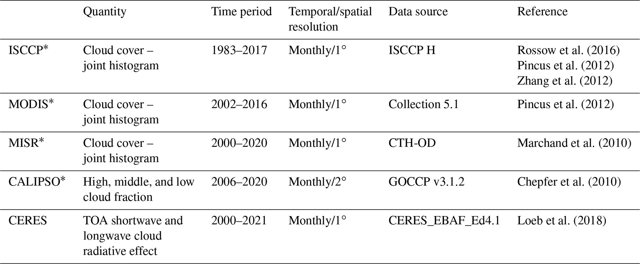
^* The joint histogram of cloud cover (as a function of cloud-top pressure (ctp) or cloud-top height (cth) and optical thickness (Tau)) and CALIPSO cloud data are from the CFMIP GCM Simulator-Oriented cloud products developed and can be downloaded from http://climserv.ipsl.polytechnique.fr/cfmip-obs/ (last access: 12 January 2023).

2.2 Satellite data

Satellite measurements from ISCCP, MODIS, MISR, and CALIPSO are used to evaluate clouds simulated by E3SMv2. CERES-EBAF Edition 4.1 data are used to evaluate the model-simulated top-of-the-atmosphere (TOA) shortwave cloud radiative effect (SWCRE) and longwave cloud radiative effect (LWCRE). More detailed information and references about these data are given in Table 1. Zhang et al. (2019) discussed additional details about these measurements. Here we highlight some of the key points from Zhang et al. (2019) to facilitate interpreting the results of this study.

Measurements from the ISCCP, MODIS, and MISR are from passive instruments. They contain information about the area coverage of clouds stratified by cloud-top pressure (ctp) or cloud-top height (cth) of the highest cloud in a column and by the column-integrated cloud optical thickness (Tau), which can be summarized in joint histograms of ctp-tau or cth-tau. As discussed in earlier studies (Marchand et al., 2010; Pincus et al., 2012), notable differences are found in the joint histograms among the three data sets, which are largely due to instrument limitations and different algorithms used for detecting clouds and retrieving the cloud heights and optical depths. For example, the ISCCP often has difficulties in detecting small cumulus clouds and mistakenly puts optically thin cirrus as a mid-topped cloud when there are low clouds underneath (Mace et al., 2006). In contrast, the retrievals used in MODIS do not work well for low-level clouds under temperature inversions or broken low-level clouds (Pincus et al., 2012), although MODIS cloud data are usually considered the most accurate for high-topped cloud among the three passive instruments. In addition, partly cloudy pixels are excluded in MODIS, while they are treated as homogeneous and included in ISCCP-detected cloud. Pincus et al. (2012) found that this could lead to 15 % difference in the optically thinnest clouds estimated by ISCCP and MODIS. Compared to ISCCP and MODIS, MISR gives the most accurate estimate of cloud-top height for low-level clouds and a better detection of cumulus clouds. Different from ISCCP, MODIS, and MISR, CALIPSO uses active instruments to measure cloud height directly and therefore can provide information of cloud vertical structure. The CALIPSO data used in this study include high-, middle-, and low-cloud fraction derived from the attenuated backscattered profile at 532 nm (Chepfer et al., 2010). Like Zhang et al. (2019), this study utilizes all these available observations to provide more complete information on model-simulated clouds.

Table 2 Description of simulations.

2.3 Sensitivity tests

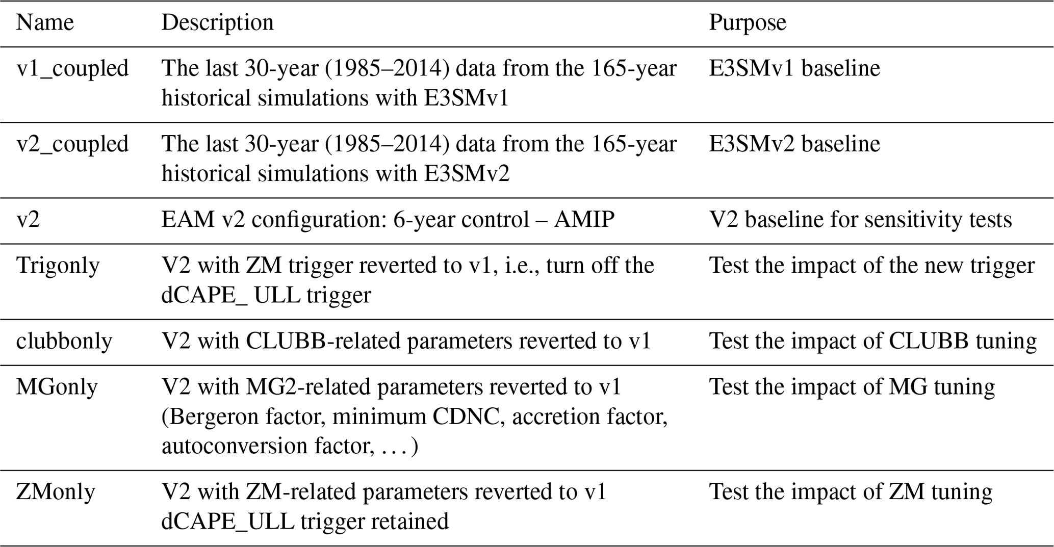
Table 2 lists the simulations analyzed in this study. In addition to the last 30-year (1985–2014) data from the 165-year historical simulations with E3SMv1 and E3SMv2 (Golaz et al., 2019, 2022) used to document the overall features of clouds simulated in these models, we also analyze the sensitivity tests with the atmosphere model of E3SMv2 (EAMv2) to investigate the impact of each major change on the simulated clouds. Four major changes made in E3SMv2 were tested in Qin et al. (2023) and analyzed in this study. They include the new dCAPE_ULL convective trigger (Trigonly) and the tuning done in CLUBB (clubbonly), MG2 (MGonly), and ZM (ZMonly). As demonstrated in Xie et al. (2019), the dCAPE_ULL trigger effectively suppresses daytime suspicious deep convection, particularly over land, and captures elevated nocturnal convection above the boundary layer. It also considerably reduces convective precipitation over subtropical regions and the occurrence frequency of light-to-moderate precipitation. The changes in model convection can have a large impact on the simulated clouds given the strong connection between clouds and convection. The tuning done in CLUBB is mainly to improve both stratocumulus and cumulus clouds and the transitions from stratocumulus to cumulus (Ma et al., 2022). As described in Table A1 of Golaz et al. (2022), the goal is achieved by (1) weakening the turbulence mixing in the planetary boundary layer (PBL) through adjusting a set of relevant parameters (e.g., clubb_c1, c14, and c6), (2) promoting cloud formation by reducing the width of the w′ probability distribution function (PDF) via reducing gamma_coef and gamma_coefb, (3) increasing stratocumulus clouds and reducing cumulus clouds by reducing skewness (skw) via increasing C8, and (4) allowing larger horizontal variation in subgrid characteristics by enlarging the difference in parameter values between high- and low-skewness regimes. The major recalibrations of cloud microphysics (MG2) include resetting the overly suppressed tuneable scaling factor (0.1) for the Wegener–Bergeron–Findeisen (WBF) process in EAMv1 to 0.7 to improve the simulation of mixed-phase clouds, adding a minimum cloud droplet number concentration (CDNC) to reduce aerosol forcing, and adjusting the exponent coefficient and the liquid cloud accretion enhancement factor to better represent clouds and precipitation in subtropical low-cloud regimes. In the deep-convection scheme (ZM), the parcel buoyancy considers the subgrid temperature perturbation from the CLUBB scheme in addition to a constant value of 0.8 K used in EAMv1. A new tunable parameter with a default value of 2.0, zmconv_tp_fac (see Table A1), is introduced to scale the square root of the CLUBB subgrid temperature variance to be the subgrid temperature perturbation. Additionally, the parameters related to the autoconversion rate, detrained ice cloud effective radius, and cloud fraction in deep convective clouds are reduced, while the parameters related to the downdraft mass flux fraction and the impact of the surface temperature change are enhanced compared to EAMv1. More details about what parameters were tuned in v2 are given in the Table A1 of Golaz et al. (2022). All the sensitivity tests are 6-year AMIP-type runs with present-day (2010) forcing from the Intergovernmental Panel on Climate Change (IPCC) AR5 emission data set (Lamarque et al., 2010), along with climatological sea surface temperature and sea ice prescribed from the observations (repeating seasonal cycle without interannual variability). To accurately measure their impacts, the same 6-year AMIP runs were conducted for the default E3SMv2. The last 5 years from each run is analyzed. By comparing the AMIP runs with the 30-year coupled simulations, the short-term AMIP runs can reproduce the major model errors shown in the long-term coupled simulations well (not shown). This suggests that the E3SM cloud behaviors should be mostly controlled by its atmosphere model, and most systematic errors in clouds are apparent in the first few years of the AMIP runs since clouds are associated with fast physics (e.g., Xie et al., 2012; Ma et al., 2014; and Qian et al., 2018).

3 General cloud features simulated in E3SMv1 and E3SMv2

Results shown in this section are based on the last 30-year (1985–2014) data from the 165-year historical simulations, which are part of the E3SMv1 and E3SMv2 CMIP6 DECK and historical simulation campaigns (Eyring et al., 2016). The exception is for MODIS simulator output. A bug was found in the MODIS simulator output shortly after the 165-year historical simulations were completed. Therefore, the results from MODIS analyzed here are from the default E3SMv1 and E3SMv2 simulations conducted in the sensitivity tests, that is, the 6-year AMIP runs. As we will discuss later, the 6-year AMIP runs can represent the general features in cloud simulations well, as we see in the 30-year coupled runs. So, we do not expect this issue will affect what we will learn from this study. In this section, we will emphasize the overall features in clouds simulated in E3SMv2 by utilizing COSP. We focus on annual mean climatology of clouds simulated by both models and changes from E3SMv1 to E3SMv2.

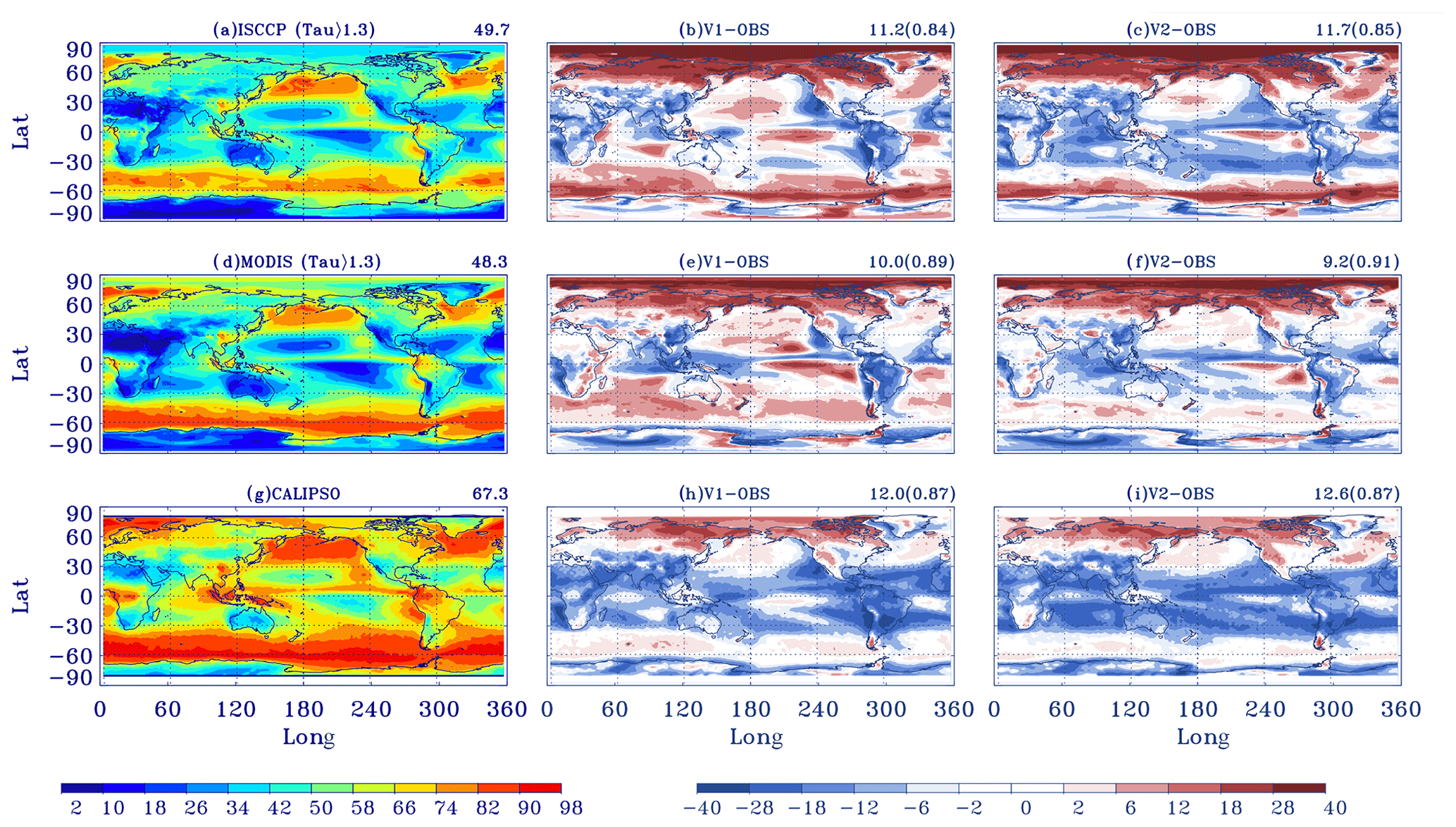
Figure 1 Annual mean total cloud fraction from (a) ISCCP (Tau >1.3), (d) MODIS (Tau >1.3), and (g) CALIPSO; the differences between E3SMv1 and observations (b), (e), and (h); and the differences between E3SMv2 and observations (c), (f), and (i). The number after each panel name is the global annual mean of cloud fraction for observations or the global annual mean RMSE and correlation (in parentheses) for cloud fraction differences.

3.1 Evaluation of model cloud with COSP

3.1.1 Total cloud fraction

The annual mean total cloud fraction between the models and the ISCCP, MODIS, and CALIPSO observations is shown in Fig. 1. Note that clouds with Tau <1.3 in ISCCP and MODIS are neglected due to the large uncertainty of cloud detection from passive instruments as discussed earlier (Marchand et al., 2010; Pincus et al., 2012). The impact of the exclusion of the optically thin clouds in ISCCP and MODIS was discussed by Zhang et al. (2019). In general, the omission of the optically thin clouds leads to a noticeable reduction in total cloud fraction between 60^∘ S and 60^∘ N; however, the exclusion of the optically thin clouds in MODIS has a minor effect on its total cloud fraction (not shown). Beyond 60^∘ S and 60^∘ N, measurements from the passive instruments are less reliable due to their difficulties in detecting clouds over surfaces with ice and snow (Klein et al., 2013; Zhang et al., 2019), and therefore caution needs to be taken for model results discussed in these regions.

Overall, both models produce comparable results with slightly fewer clouds simulated in E3SMv2 compared to its previous version. E3SMv2 generally shows slightly larger errors than E3SMv1 compared to ISCCP and CALIPSO. Relative to ISCCP, E3SMv2 underpredicts clouds in the tropical and extratropical regions and has more clouds over the Arctic than observations. As we will show later, this is mainly related to its simulated low clouds. E3SMv1 shows a similar error pattern in most regions except for the Pacific Ocean where clouds are generally overestimated. Relative to CALIPSO, both models underpredict clouds globally except for the Arctic. Compared to MODIS, however, E3SMv2 shows a slightly better result than E3SMv1 with reduced biases over most regions. The discrepancy in model performance against different satellite data is likely not due to the use of 6-year AMIP simulations for MODIS since a similar discrepancy is seen when 6-year simulation data are used for ISCCP and CALIPSO (not shown).

A robust improvement made in E3SMv2 is the considerable increase in stratocumulus cloud over the eastern ocean basins along the coasts, such as the west coasts of southern Africa and North and South America. The comparison with all three satellite observations shows this improvement. This is significant since the lack of stratocumulus along the coasts in E3SMv1 (common in most climate models) is one of the main outstanding issues that the development of E3SMv2 tackled. Cloud biases over N. Hemisphere storm tracks, the stratocumulus-to-cumulus transition regimes, and the Southern Ocean (SO) are also noticeably reduced in E3SMv2, as seen in the comparisons, particularly with ISCCP and MODIS. It is worth mentioning that the marine stratocumulus cloud biases are substantially reduced in the E3SMv2 North American regionally refined configuration (Tang et al., 2023), i.e., the high-resolution version of the E3SMv2 release. This is due to the finer resolutions in both atmosphere and ocean and highlights the benefits of refining resolutions in multiple components than in a single component.

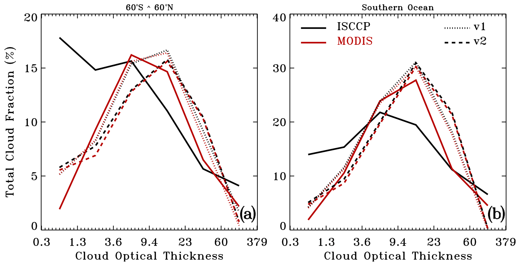
Figure 2 Column-integrated cloud optical depth distributions averaged (a) over 60^∘ S–60^∘ N and (b) over Southern Ocean (45–60^∘ S) for ISCCP, MODIS, E3SMv1, and E3SMv2.

The model-simulated clouds are further examined by analyzing the column-integrated cloud optical depth distributions for total cloud fraction averaged in the domain between 60^∘ S and 60^∘ N and over the SO region between 45 and 60^∘ S, respectively (Fig. 2). The domain between 60^∘ S and 60^∘ N is selected because measurements from ISCCP and MODIS are more reliable while the SO region is selected since most climate models have difficulties in accurately capturing clouds over this region where E3SMv2 shows clearly improvements in cloud simulations compared to E3SMv1. ISCCP and MODIS agree relatively better for clouds with Tau >3.6, while for clouds with Tau <3.6, the total cloud fraction in ISCCP is significantly larger than that in MODIS, primarily due to the different assumptions on partly cloudy pixels in their retrievals (Zhang et al., 2019). For 3.6< Tau <23, MODIS shows larger cloud fraction than ISCCP. In contrast, model results from the two simulators are very close to each other. This is because ISCCP and MODIS simulators use nearly the same method to determine the values of Tau (Pincus et al., 2012).

Both models agree with MODIS much better than with ISCCP in both examined regions. Relative to MODIS, E3SMv1 reproduces optically thin clouds generally well (1.3< Tau <3.6) and notably overestimates optically intermediate to thick clouds (Tau ≧9.4). In contrast, E3SMv2 underpredicts the optically thin clouds and shows slightly larger overestimation of thick clouds (Tau >23) compared to E3SMv1. The largest discrepancy between E3SMv1 and v2 is seen for Tau between 3.6 and 9.4, where E3SMv2 performs worse than v1 and considerably underestimates the MODIS observed clouds. This suggests that some features seen in the total cloud fraction in Fig. 1 are the result of compensating errors in clouds with different optical properties. For example, the reduction in positive cloud fraction bias over the SO in E3SMv2 relative to MODIS, as shown in Fig. 1, appears to stem more from the deficiencies in optically thin and intermediate clouds than the slightly more excessive optically thick clouds with respect to E3SMv1.

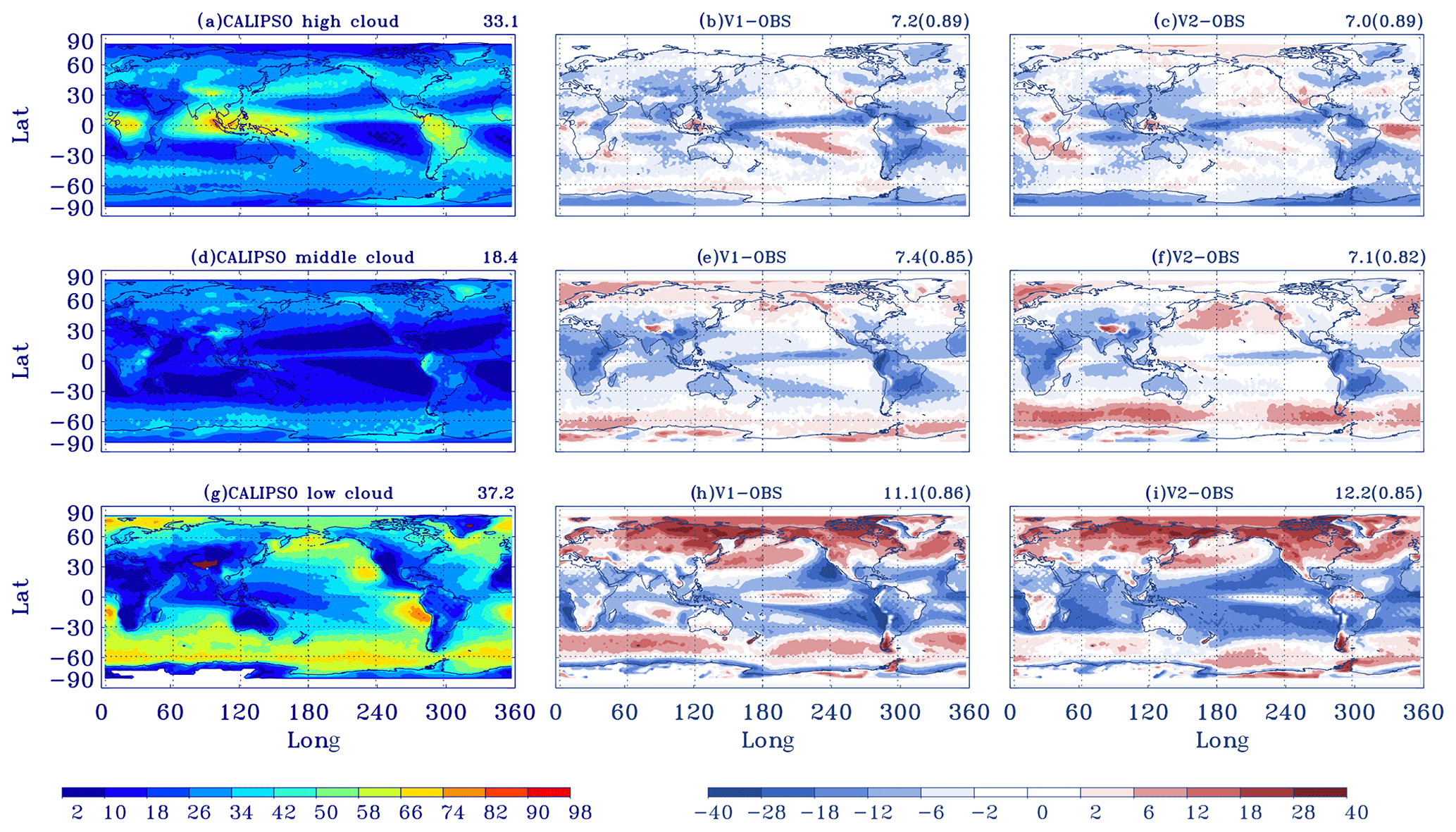
Figure 3 Annual mean CALIPSO-derived (a) high-, (d) middle-, and (g) low-cloud fraction; the differences between E3SMv1 and observation for (b), (e), and (h); and the differences between E3SMv2 and observation for (c), (f), and (i). The number after each panel name is the global annual mean of cloud fraction for observations or the global annual mean RMSE and correlation (in parentheses) for cloud fraction differences.

3.1.2 Cloud vertical structure

The annual mean high-, middle-, and low-cloud fractions from CALIPSO and model biases from the observation are shown in Fig. 3. The high, middle, and low clouds in both models and CALIPSO are defined as having a cloud-top pressure lower than 440 hPa, between 440 and 680 hPa, and higher than 680 hPa, respectively. E3SMv1 and E3SMv2 show similar bias patterns for all types of clouds, with clouds at all heights mostly underpredicted in the low latitudes and low clouds overpredicted in the northern high latitudes and the SO. Over the tropics, E3SMv2 slightly improves high and middle clouds, with a noticeable reduction in errors in the South Pacific (high clouds) and tropical and subtropical Pacific (middle clouds), when compared with E3SMv1. On the other hand, it degrades the representation of low clouds over tropical and subtropical oceans except along the subtropical coasts in both hemispheres, where E3SMv2 produces much more stratocumulus (better). Over the SO, the overpredicted clouds in E3SMv1 are reduced in E3SMv2. The degradation of low clouds over tropical and subtropical oceans is partially due to error compensation in low clouds with different optical properties in E3SMv1, as will be shown in a comparison with the MISR low-cloud data, which give a more accurate estimate of low clouds over oceans compared to CALIPSO (Zhang et al., 2019). Also over the SO, E3SMv2 shows larger overestimation of middle-level clouds and smaller overestimation of low clouds. This breakdown of biases in terms of clouds vertical structure from CALIPSO provides additional information to understand the overall model performance in simulating total cloud fraction. For instance, the degradation of the total cloud fraction simulation in E3SMv2 over the tropical and subtropical regions as shown in Fig. 1i is primarily due to errors in low clouds since middle and high clouds are generally improved over these regions (Fig. 3c, f, and i).

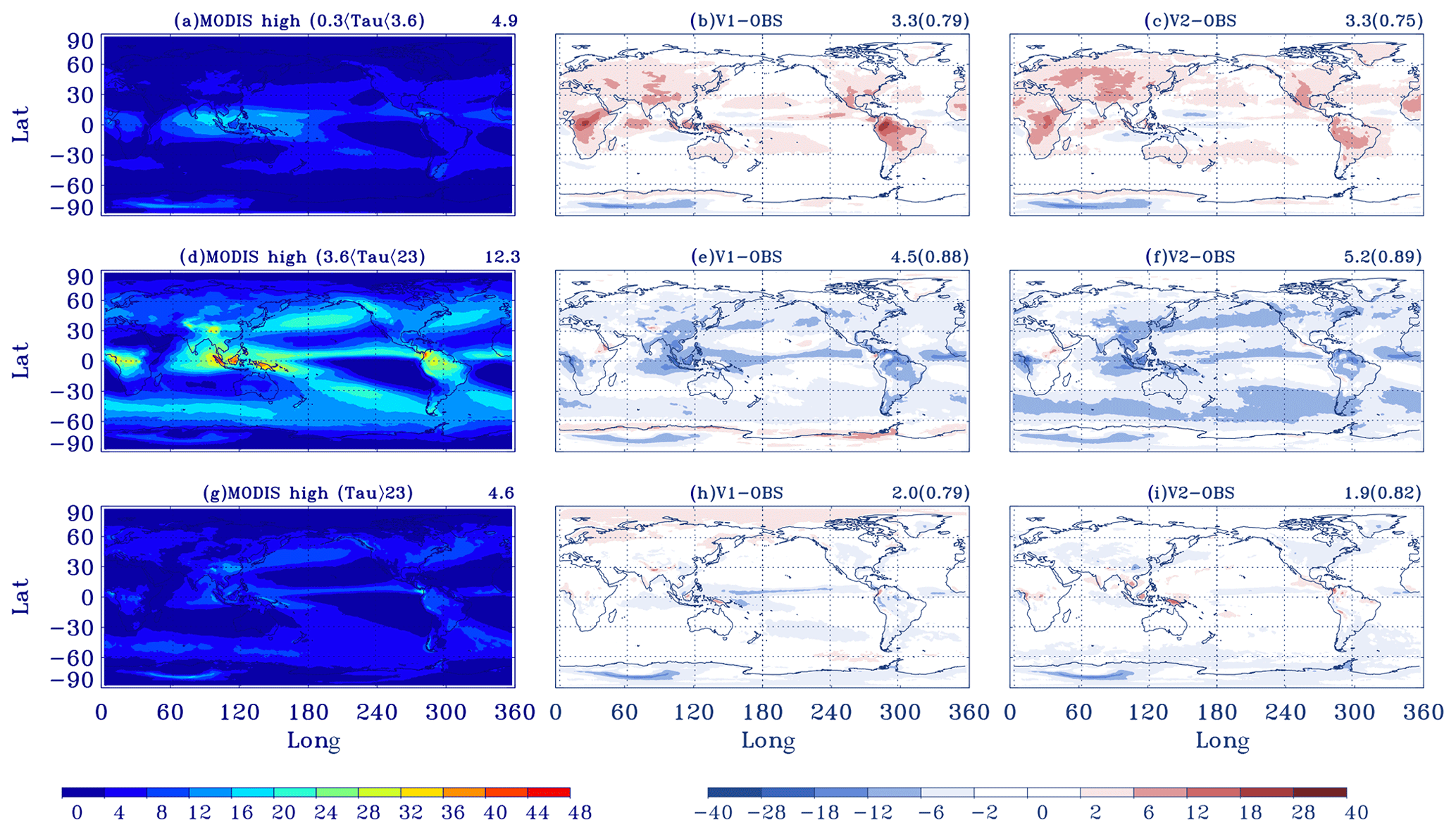
Figure 4 Annual mean MODIS high-topped thin (0.3< Tau <3.6), intermediate (3.6< Tau <23), and thick (Tau >23) clouds. Panels (a), (d), and (g) are MODIS observations; panels (b), (e), and (h) are the differences between E3SMv1 and observations; and panels (c), (f), and (i) are the differences between E3SMv2 and observations. The number after each panel name is the global annual mean of cloud fraction for observations or the global annual mean RMSE and correlation (in parentheses) for cloud fraction differences.

3.1.3 High clouds

The simulated high clouds in three optical thickness ranges (thin, intermediate, and thick) are further examined with MODIS (Fig. 4) since MODIS provides more accurate information about high clouds than other data sets. Despite some regional differences, E3SMv2 shows a very similar error pattern to E3SMv1. In general, both models overestimate the MODIS cloud fraction (particularly over land) for optically thin clouds and underestimate it (mainly over ocean) for optically intermediate and thick clouds. E3SMv2 shows slightly larger error for optically intermediate clouds and slightly smaller error for optically thick clouds. There are some improvements seen in E3SMv2 along the Antarctic coasts for optically intermediate clouds and in the Arctic for optically thick clouds, where E3SMv1 slightly overestimates the observed clouds.

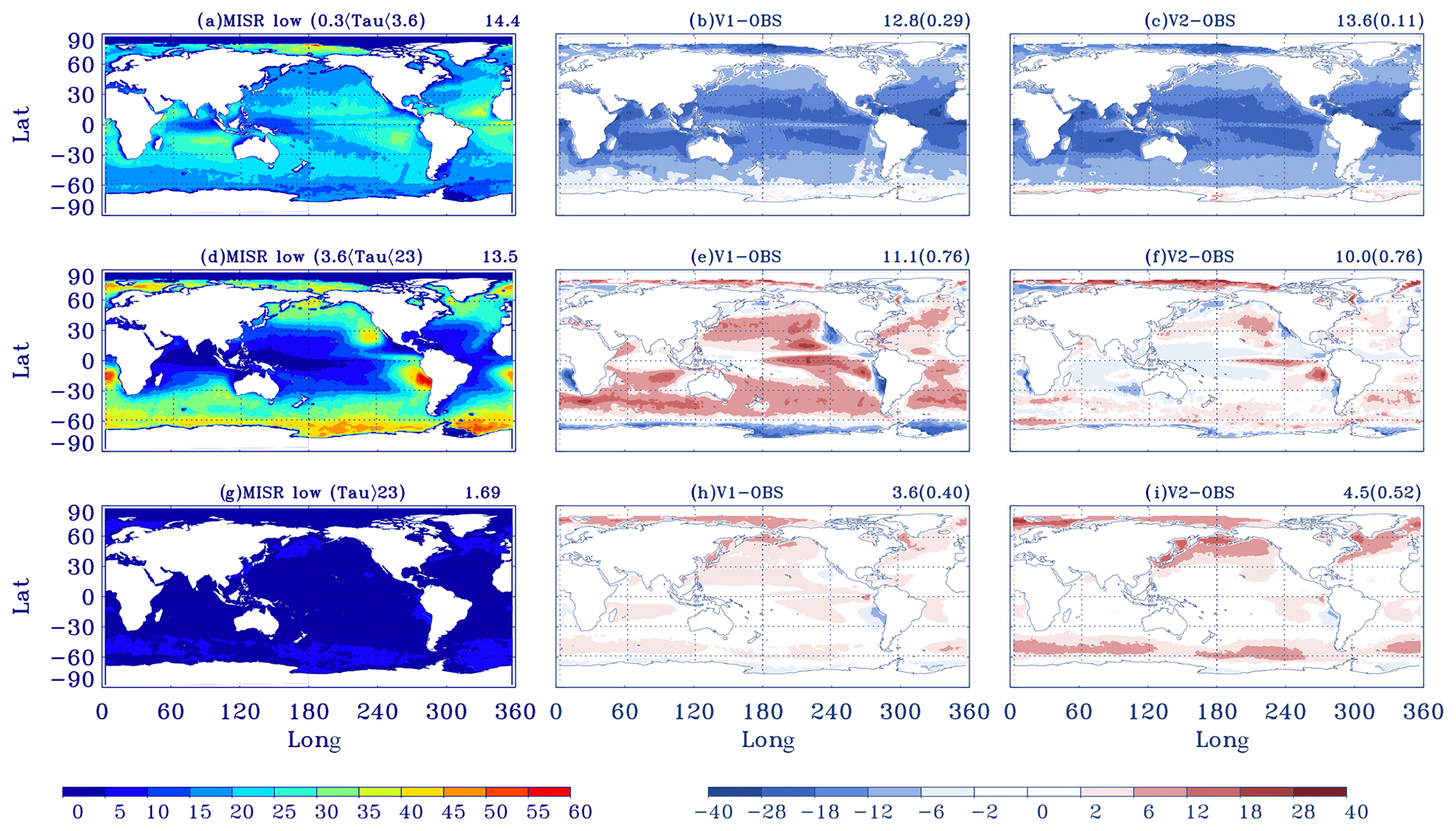
Figure 5 Annual mean MISR low-topped optically thin (0.3< Tau <3.6), intermediate thickness (3.6< Tau <23), and thick (Tau >23) clouds. Panels (a), (d), and (g) are MISR observations; panels (b), (e), and (h) are the differences between E3SMv1 and observation; and panels (c), (f), and (i) are the differences between E3SMv2 and observation. The number after each panel name is the global annual mean of cloud fraction for observations or the global annual mean RMSE and correlation (in parentheses) for cloud fraction differences.

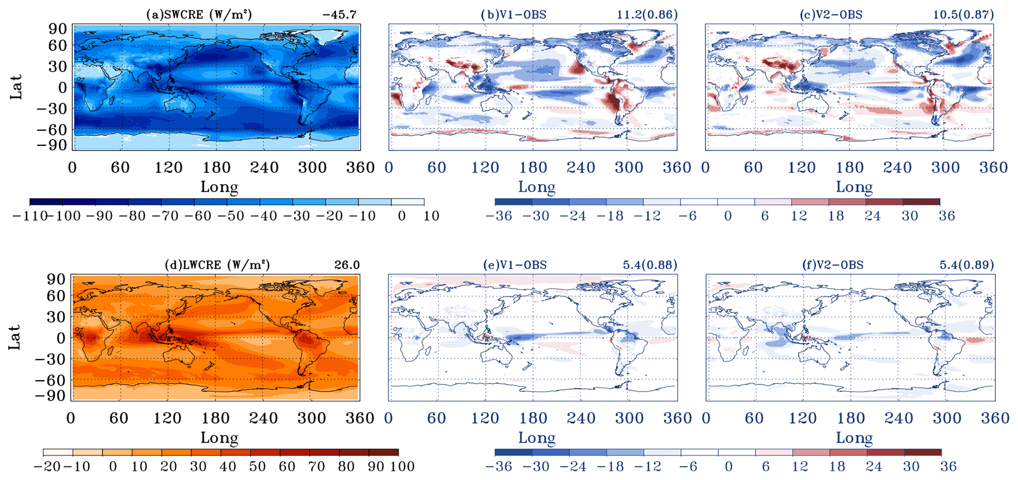
Figure 6 Annual mean (a) SWCRE and (d) LWCRE for CERES and (b) and (e) differences between E3SMv1 and CERES and (c) and (f) between E3SMv2 and CERES. The number after each panel name is the global annual mean of CRE for observations or the global annual mean RMSE and correlation (in parentheses) for cloud fraction differences.

3.1.4 Low clouds

As MISR can detect low clouds well, it is used to provide additional insights into model deficiencies in simulating low clouds. The optically thin, intermediate, and thick low-cloud fractions (cth below 3 km) from MISR (only available over oceans) and the difference between the models and MISR are displayed in Fig. 5. For optically thin low clouds (0.3< Tau <3.6), there is little change in model errors from E3SMv1 to E3SMv2. Both models largely underestimate the optically thin low clouds in both tropical and midlatitude oceans. For optically intermediate low clouds (3.6< Tau <23), E3SMv2 dramatically improves the simulation. The large overestimation over the Northern Hemisphere storm tracks, the SO, and the stratocumulus-to-cumulus transition regimes and underestimation in the stratocumulus regions in E3SMv1 are significantly reduced in E3SMv2, consistent with the earlier discussions and Golaz et al. (2022). However, the smaller positive biases in optically intermediate low clouds in E3SMv2 lead to a bigger negative bias in total low-cloud fraction than E3SMv1, as shown in Fig. 3 (compared to CALIPSO low clouds). The better performance shown in E3SMv1 is clearly due to error compensation between its simulated optically thin (underestimated) and intermediate (overestimate) low clouds. The optically thick low clouds are not the dominant cloud type. Only a few optically thick low clouds are detected by MISR, for which the models show a slightly positive bias in the N. Hemisphere storm tracks and the SO, especially for E3SMv2.

3.2 Cloud radiative effect

Clouds have a large impact on radiation. The biases in the model-simulated SWCRE and LWCRE from the CERES-EBAF Ed4.1 data set (Fig. 6) are closely related to those in model clouds. SWCRE is largely influenced by low clouds. The most noticeable improvement from E3SMv1 to E3SMv2 is over the stratocumulus regimes along the west coast of continents where the severely underestimated SWCRE in E3SMv1 is significantly reduced due to the improvement of stratocumulus as discussed earlier. In contrast, the biases in LWCRE are more related to high clouds. The major error in E3SMv1 is the much weaker LWCRE due to large underestimation of (optically intermediate) high clouds over the tropical Indo-West Pacific region (Fig. 4e and f). This problem is reduced over the western Pacific region in E3SMv2, while it is slightly exaggerated over eastern Indian Ocean. For other regions, the change is little from E3SMv1 to E3SMv2.

4 Impact of major changes in v2 on cloud simulations

The previous section indicates that E3SMv2 largely improves the stratocumulus clouds over the eastern ocean basins in both hemispheres along the coast of southern Africa and North and South America, along with the improvement seen in the stratocumulus-to-cumulus transition regimes, and the SO, while it degrades the simulations of high clouds and total cloud fraction compared to E3SMv1. The improvements in low clouds are mainly from optically intermediate clouds with Tau in a range of 3.6 and 23. For optically thin (Tau <0.3) and thick (Tau >23) low clouds, E3SMv2 actually produces a slightly worse result. The degradation of high clouds is primarily from the intermediate clouds.

In this section, we discuss what changes made in E3SMv2 have led to these changes in clouds from E3SMv1 to E3SMv2 through carefully designed sensitivity experiments, which are shown in Table 2 and discussed in Sect. 2.3. Since model responses to these changes are similar regardless of which simulator output is used, for simplicity, we use MODIS for total cloud fraction and CALIPSO for vertical cloud structure. Results from both MODIS and MISR simulators are also examined and discussed in this section for high and low clouds, respectively, given their relatively more accurate measurements in these two types of clouds. The inclusion of MODIS and MISR clouds is particularly meaningful to aid in the breakdown of the model responses in terms of cloud opacity. The relevant figures for MODIS high clouds and MISR low clouds are included in Appendix.

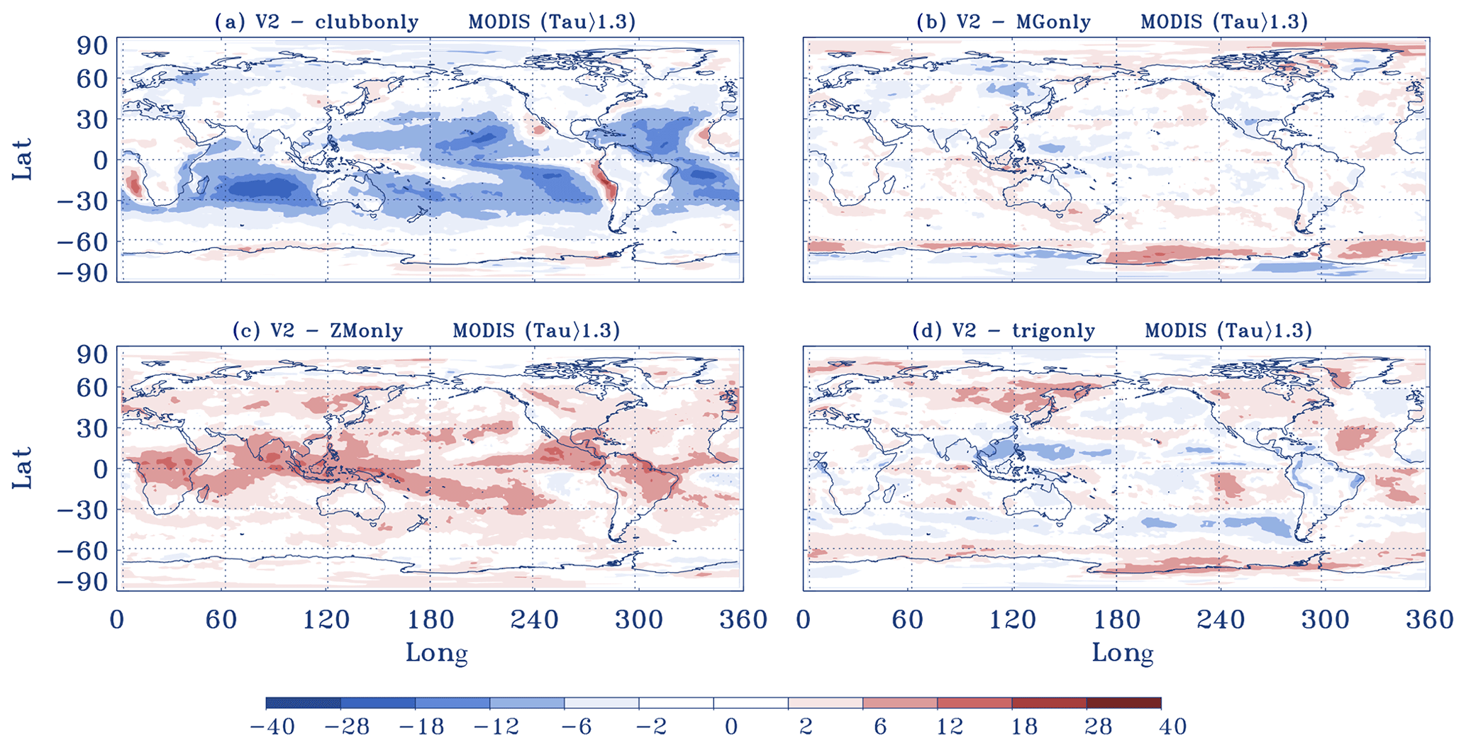
Figure 7 Difference in cloud fraction from the MODIS simulator (Tau >1.3) between sensitivity tests and the default E3SMv2 run. (a) E3SMv2 with CLUBB-related parameters changed from v2 to v1, (b) E3SMv2 with MG2-related parameters changed from v2 to v1, (c) E3SMv2 with ZM-related parameters changed from v2 to v1, and (d) E3SMv2 with the dCAPE_ULL trigger turned off. All results are from 6-year AMIP-style climatology runs.

4.1 MODIS total cloud fraction

Figure 7 shows the impact of these changes on the simulation of total clouds. The improved stratocumulus along the west coast of southern Africa and North and South America is clearly due to the retuning of CLUBB, which promote stratocumulus-like symmetric mixing by increasing the damping coefficients and allowing larger horizontal variation in subgrid vertical velocity as described in Ma et al. (2022). However, the retuning of CLUBB also leads to a considerable reduction in clouds over tropical and subtropical oceans, which contributes to the fewer clouds produced in E3SMv2 compared to v1. This is mainly from tuning those parameters that can decrease boundary layer mixing and decoupling between boundary layer and free troposphere. The cloud lateral entrainment is also decreased in v2 due to the CLUBB retuning, which could lead to a reduced cloudiness in shallow cumulus regime. As indicated by CALIPSO (Figs. 9–11) and MISR (Figs. A1–A3), the CLUBB-induced cloud changes are mainly in the optically intermediate low clouds. The reduction in total clouds is partially offset by the tuning done in ZM, which extends clouds originated from deep convection to almost everywhere. This is largely due to the tuning of the autoconversion for convective clouds, which is significantly tuned down from 0.007 in E3SMv1 to a nominal value of 0.002 in E3SMv2. This increases cloud condensate amount detrained from deep convection and increases overall cloudiness. An analysis of MODIS high clouds (Figs. A4–A6) supports that the major impact on high clouds is from the ZM tuning, which largely increases the optically intermediate and thick clouds. The impact of MG2 tuning and the new convective trigger on total cloud fraction is relatively small compared to the tuning done in CLUBB and ZM. The MG2 tuning mainly influences high latitudes, particularly along the Antarctic coastline, while the new trigger produces more clouds over most of the regions, except for the tropical western Pacific and the SO between 30 and 60^∘ S, where a reduction in clouds is noticeable. The large impact of MG2 tuning on high-latitude clouds is likely due to the change in the WBF process rate, which has a large impact on mixed-phase clouds that are common in high latitudes.

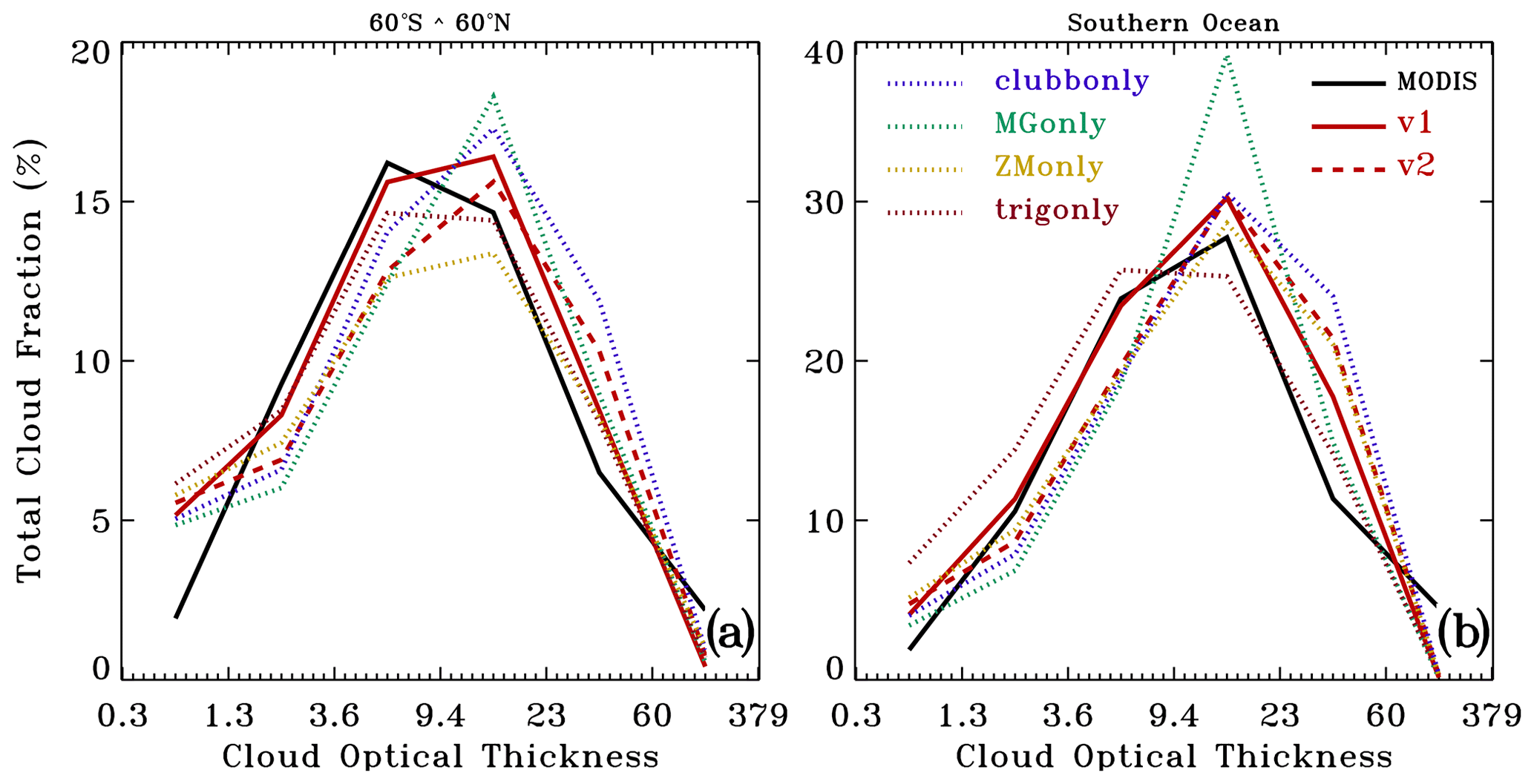
Figure 8 Column-integrated cloud optical depth distributions averaged (a) over 60^∘ S–60^∘ N and (b) over the Southern Ocean (45–60^∘ S) for MODIS, E3SMv1, E3SMv2, and sensitivity tests.

The impact on total cloud fraction with different cloud optical properties is further examined in Fig. 8. Over 60^∘ S–60^∘ N, consistent with Fig. 7, the CLUBB tuning has led to a reduction in clouds regardless of their optical properties, which results in a better simulation of optically thick clouds (Tau >9.4) and a worse simulation of optically thin clouds (Tau ≦9.4). The ZM tuning response is to increase clouds with an overall minor impact on optically thin clouds (Tau <3.6) and a considerably large impact on clouds with cloud optical depth between 3.6 and 23 that are more relevant to deep convection. The MG tuning mainly affects simulation of intermediate clouds (3.6< Tau <23), where the overestimation of clouds is reduced. The impact of the new trigger on clouds is more clearly demonstrated when examining clouds with different optical properties. It acts to reduce optically thin clouds and increase optically intermediate and thick clouds. This is consistent with Xie et al. (2019), who showed that the new trigger helped suppress light precipitation and enhance intermediate and heavy precipitation.

Similar impacts of these changes are found over the SO. The tuning done in CLUBB helps bring optically intermediate and thick clouds (Tau >9.4) closer to the observations, and the MG tuning dramatically improves optically intermediate clouds (9.4< Tau <23). The new trigger acts to reduce optically thin clouds and increase optically intermediate and thick clouds like over 60^∘ S to 60^∘ N. The reduction in optically thin clouds from the new trigger is mainly from low clouds as indicated in Fig. A1d. The exception is for the ZM tuning, which has a minor impact over the SO.

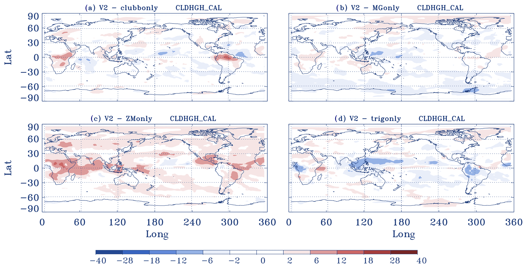
Figure 9 Difference in high-cloud fraction from the CALIPSO simulator between sensitivity tests and the default E3SMv2 run. (a) E3SMv2 with CLUBB-related parameters changed from v2 to v1, (b) E3SMv2 with MG2-related parameters changed from v2 to v1, (c) E3SMv2 with ZM-related parameters changed from v2 to v1, and (d) E3SMv2 with the dCAPE_ULL trigger turned off. All results are from 6-year AMIP-style climatology runs.

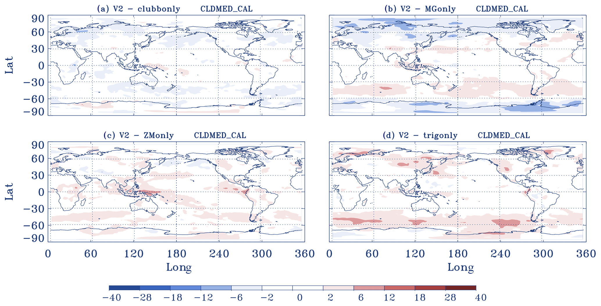
Figure 10 Difference in middle-level cloud fraction from the CALIPSO simulator between sensitivity tests and the default E3SMv2 run. (a) E3SMv2 with CLUBB-related parameters changed from v2 to v1, (b) E3SMv2 with MG2-related parameters changed from v2 to v1, (c) E3SMv2 with ZM-related parameters changed from v2 to v1, and (d) E3SMv2 with the dCAPE_ULL trigger turned off. All results are from 6-year AMIP-style climatology runs.

4.2 CALIPSO vertical cloud structure

Figures 9–11 display the impact of these changes on the simulation of high, middle, and low clouds, respectively. For high clouds (Fig. 9), it is not surprising to see that the deep-convection ZM tuning has the largest impact, which considerably increases high clouds globally, especially in the tropics. The new trigger leads to a considerable reduction in high clouds over the western Pacific, which is consistent with the reduction in precipitation over this region as shown in Xie et al. (2019). The CLUBB tuning typically increases high clouds over land and reduces them over ocean. Overall, the impact of MG2 on high clouds is minor, with a slight increase in clouds in the Arctic and reduction in clouds along the Antarctic coastlines. By comparing with MODIS high clouds, the changes in high clouds are mainly in intermediate and thick clouds due to the changes in ZM (Figs. A5c and A6c). All the changes have minor impact on optically thin high clouds.

For middle clouds (Fig. 10), the CLUBB tuning leads to a slight reduction in cloud amount globally. The MG2 tuning leads to a considerable reduction in clouds in both Arctic and Antarctic and a slight increase in clouds over the SO. The impact of the ZM tuning and the new trigger is mainly to increase clouds in the tropics (the ZM tuning) and the SO and the Arctic regions (the new trigger).

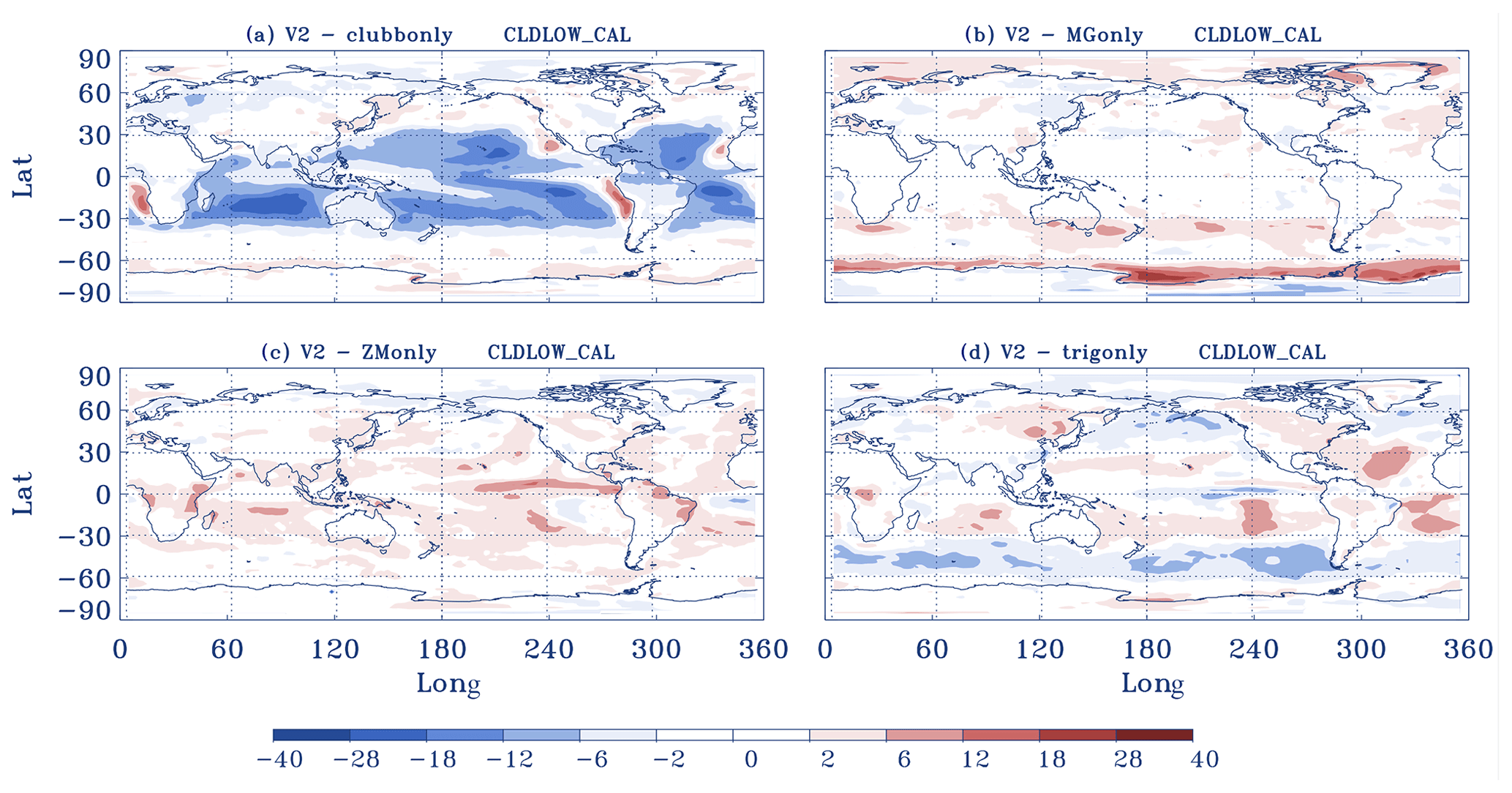
Figure 11 Difference in low-cloud fraction from the CALIPSO simulator between sensitivity tests and the default E3SMv2 run. (a) E3SMv2 with CLUBB-related parameters changed from v2 to v1, (b) E3SMv2 with MG2-related parameters changed from v2 to v1, (c) E3SMv2 with ZM-related parameters changed from v2 to v1, and (d) E3SMv2 with the dCAPE_ULL trigger turned off. All results are from 6-year AMIP-style climatology runs.

For low clouds (Fig. 11), the CLUBB tuning plays the largest role in the E3SMv2 cloud changes. It dramatically reduces the low clouds in the tropical and subtropical regions except for the stratocumulus regime, where low clouds along the subtropical coasts largely increase. These changes are primarily from the optically intermediate clouds as indicated earlier. The tuning done in ZM, as well as the use of the new trigger, helps offset the reduction in clouds made by the CLUBB tuning over the tropical and midlatitude regions. The exception is over the SO where the new trigger acts to reduce low clouds and MG2 tuning to substantially increase low clouds around the Antarctica. The reduced low clouds by the new trigger are mainly from optically thin clouds, while the increased low clouds by MG2 are from optically thin and thick clouds suggested by MISR.

The analysis of the vertical cloud structure clearly indicates the compensation effect of cloud changes in the vertical that has an impact on the total cloud fraction, shown in Fig. 7. For instance, the opposite sign of changes in middle and low clouds over the SO with the new trigger leads to overall small changes over that region in Fig. 7.

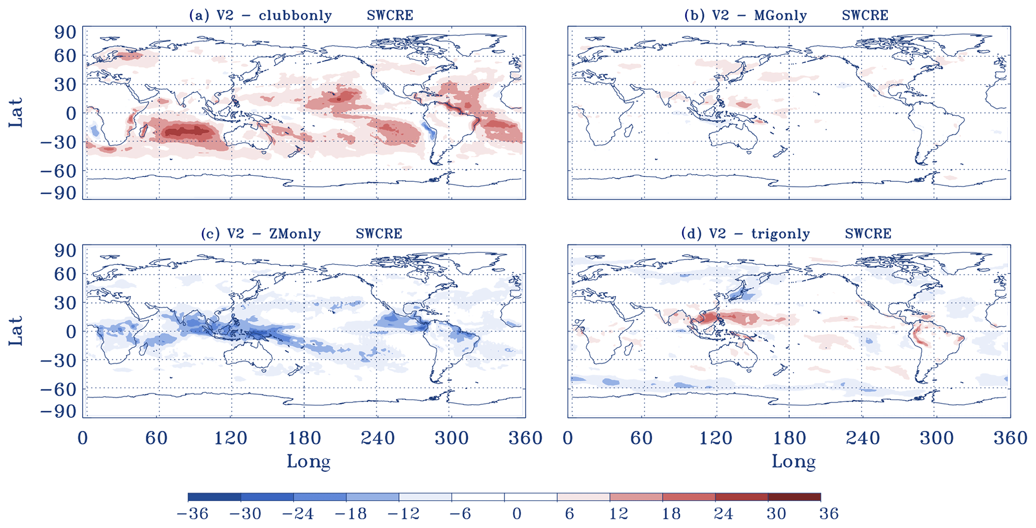
Figure 12 Difference in SWCRE (W m⁻²) between sensitivity tests and the default E3SMv2 run. (a) E3SMv2 with CLUBB-related parameters changed from v2 to v1, (b) E3SMv2 with MG2-related parameters changed from v2 to v1, (c) E3SMv2 with ZM-related parameters changed from v2 to v1, and (d) E3SMv2 with the dCAPE_ULL trigger turned off. All results are from 6-year AMIP-style climatology runs.

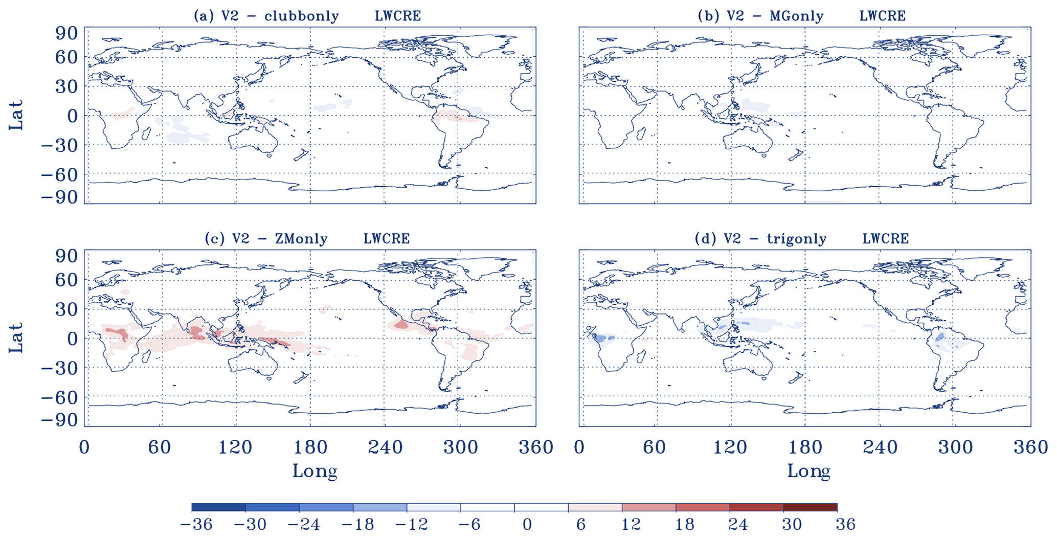
Figure 13 Difference in LWCRE (W m⁻²) between sensitivity tests and the default E3SMv2 run. (a) E3SMv2 with CLUBB-related parameters changed from v2 to v1, (b) E3SMv2 with MG2-related parameters changed from v2 to v1, (c) E3SMv2 with ZM-related parameters changed from v2 to v1, and (d) E3SMv2 with the dCAPE_ULL trigger turned off. All results are from 6-year AMIP-style climatology runs.

4.3 SWCRE and LWCRE

The impacts of these model changes on SWCRE and LWCRE are shown in Figs. 12 and 13, respectively. For SWCRE, consistent with the large reduction in low clouds, the CLUBB tuning largely reduces SWCRE over the tropical and subtropical oceans. In contrast, the SWCRE in the tropical deep-convection regions becomes much stronger, mainly due to the increase in optically intermediate and thick high clouds due to the ZM tuning. The reduction in high clouds over the western Pacific with the new trigger leads to reduction in SWCRE. Overall, the impact of the MG2 tuning on SWCRE is minor.

For LWCRE, only the ZM tuning has a noticeable impact, leading to an increase in LWCRE due to the increase in high clouds. The minor impact of the CLUBB tuning in LWCRE indicates that the changes in low clouds have a minor impact on LWCRE.

5 Summary

We performed systematic evaluation of clouds simulated in the newly developed E3SMv2 with satellite observations by utilizing the satellite simulator package (COSP) to mitigate sampling and algorithmic differences between modeled and observed clouds. Multiple cloud observations measured by various instruments were used to address potential data uncertainty and instrument and retrieval limitations. Our focus is to document E3SMv2 performance on clouds and understand what updates in E3SMv2 have caused the changes in clouds from E3SMv1 to E3SMv2. For the second purpose, results from four sensitivity tests conducted in Qin et al. (2023) were used to isolate the impact of tuning done in CLUBB, MG2, and ZM and the use of the new dCAPE_ULL trigger in E3SMv2 on clouds.

In general, E3SMv2 shows a similar error pattern in clouds as exhibited in its previous version. One robust improvement is seen in the stratocumulus regime, where stratocumulus clouds along the subtropical west coast of continents in both hemispheres are largely increased. This is true by comparing all the satellite data sets used in this study and consistent with a much stronger (better) SWCRE over these stratocumulus regions. The MISR data further indicate that the improvement is mainly from optically intermediate low clouds (3.6< Tau <23) along the subtropical coasts. Note that the lack of stratocumulus clouds is one of the most outstanding problems in E3SMv1. This improvement represents a big achievement made in E3SMv2 (Golaz et al., 2022). Relative to CALIPSO, however, E3SMv2 shows a larger negative bias in total low clouds than E3SMv1 in other regions in tropical and subtropical oceans. A comparison with MISR suggests that the smaller biases in E3SMv1 partially result from error compensation in its simulated low clouds with different optical properties, for which E3SMv1 shows an underestimation of optically thin low clouds (similar to E3SMv2), while it largely overestimates optically intermediate low clouds in these regions. Relative to the large changes in low clouds, E3SMv1 and E3SMv2 show very similar simulation of CALIPSO high clouds, although some regional changes are seen in their simulated optical properties as demonstrated in comparison of MODIS.

The sensitivity tests indicate that the improved stratocumulus along the coast is primarily from the retuning of parameters related to CLUBB. Other changes only have minor contributions. However, the CLUBB tuning also resulted in a reduction in low clouds, due to the reduction in optically intermediate clouds, in the tropical and subtropical regions. This change reduced the overpredicted cumulus clouds in the subtropical cumulus regions but exaggerated the issue with underpredicted cloud in other regions in tropical and subtropical oceans. This led to an overall slight degradation of cloud simulation in E3SMv2 compared to E3SMv1, although the better performance in the latter is partially due to error compensation in clouds with different optical properties, as discussed earlier. The sensitivity tests indicate that the impact of the MG tuning on clouds is mainly in the high latitudes over both hemispheres, where it increased low clouds and decreased middle clouds. Over the SO, its overall effect is minor. However, a close look at the cloud optical properties over the SO shows a significant improvement in optically intermediate clouds compared to MODIS. Overall, its impact on clouds is smaller than the other updates examined in this study. The ZM tuning primarily increased optically intermediate and thick high clouds over the tropical deep-convection regions. The increase in the high clouds partially offset the decrease of low clouds by the CLUBB tuning in the total cloud fraction and had a positive impact on simulation of both SWCRE and LWCRE in E3SMv2 over the tropical deep-convection regions. Similar to the MG2 tuning, the impact of the new trigger on clouds is also smaller than the tuning done in CLUBB and ZM. The most noticeable change using the new trigger is the large increase in optically thick low clouds near the Antarctic coast and in the northern high latitudes, whereas changes of opposite sign are seen in its optically thin clouds produced, leading to much smaller overall changes over these areas in Fig. 11d.

This study offered additional insights into clouds simulated in E3SMv2 by utilizing multiple data sets, the COSP diagnostic tool, and sensitivity tests. The improved understanding will benefit future E3SM developments and application of E3SM in various science applications.

Appendix A

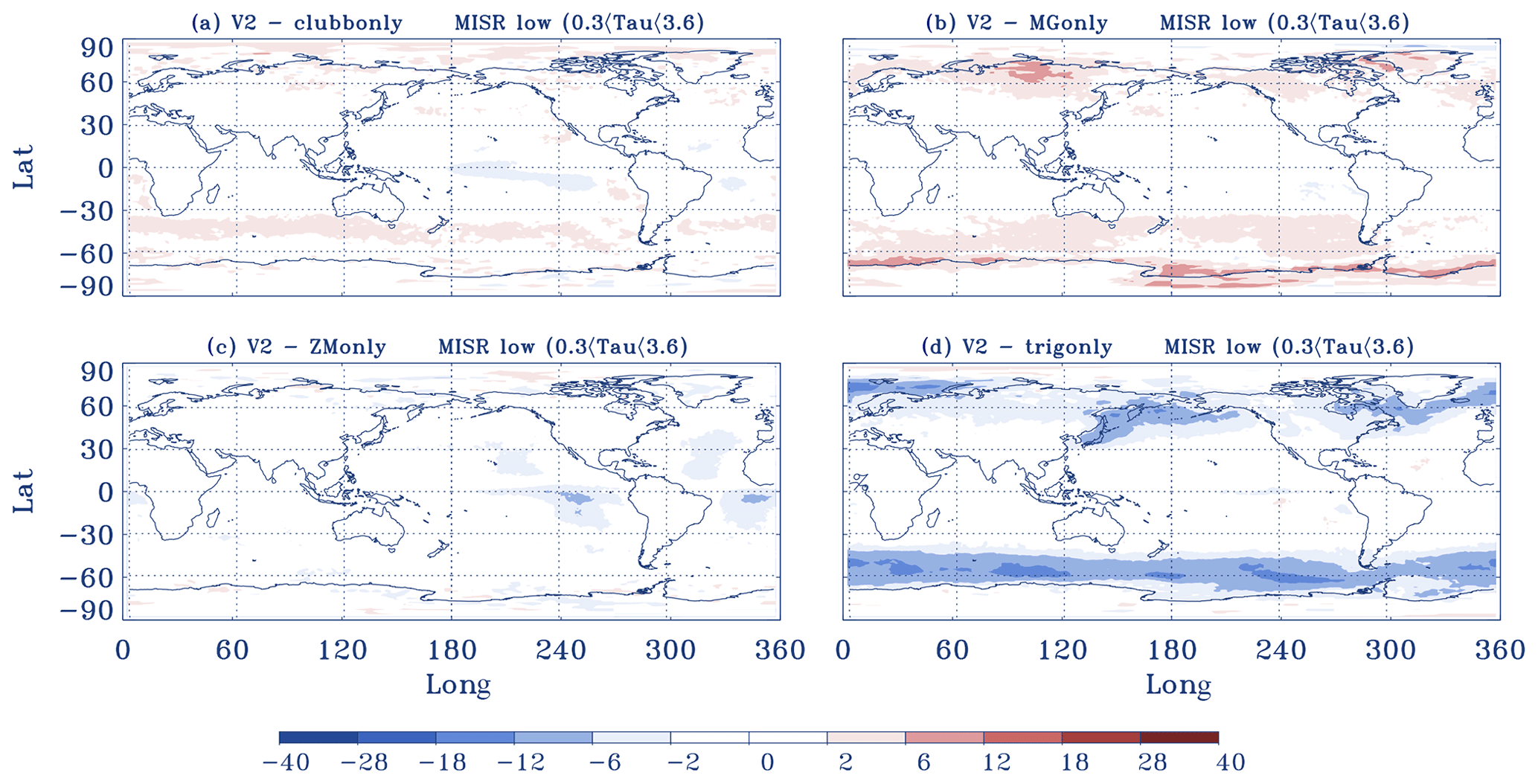
Figure A1 Difference in optically thin low-cloud fraction from the MISR simulator (0.3< Tau <3.6) between sensitivity tests and the default E3SMv2 run. (a) E3SMv2 with CLUBB-related parameters changed from v2 to v1, (b) E3SMv2 with MG2-related parameters changed from v2 to v1, (c) E3SMv2 with ZM-related parameters changed from v2 to v1, and (d) E3SMv2 with the dCAPE_ULL trigger turned off. All results are from 6-year AMIP-style climatology runs.

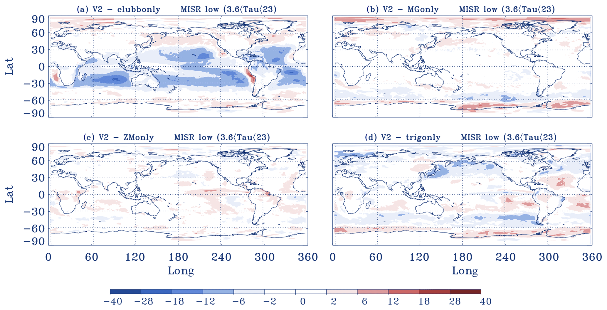
Figure A2 Difference in optically intermediate low-cloud fraction from the MISR simulator (3.6< Tau <23) between sensitivity tests and the default E3SMv2 run. (a) E3SMv2 with CLUBB-related parameters changed from v2 to v1, (b) E3SMv2 with MG2-related parameters changed from v2 to v1, (c) E3SMv2 with ZM-related parameters changed from v2 to v1, and (d) E3SMv2 with the dCAPE_ULL trigger turned off. All results are from 6-year AMIP-style climatology runs.

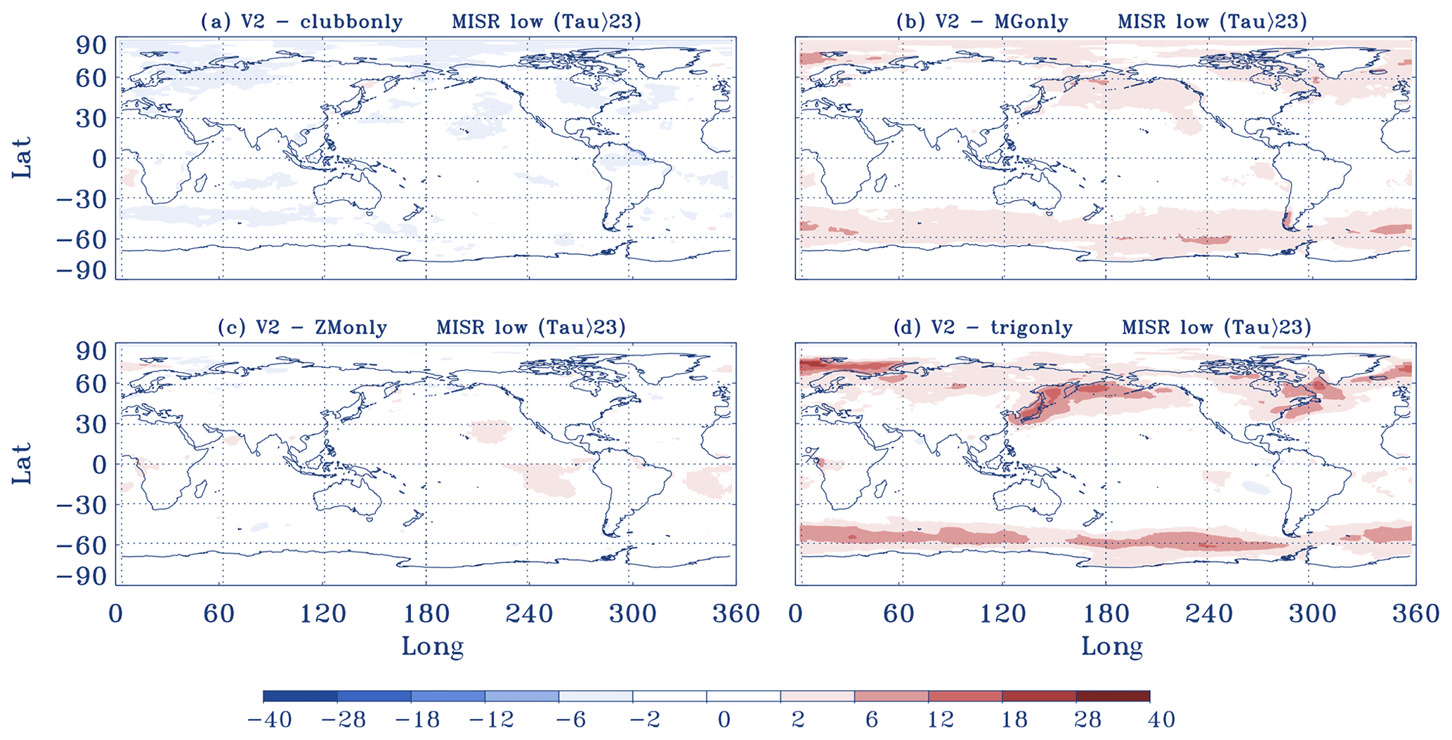
Figure A3 Difference in optically think low-cloud fraction from the MISR simulator (Tau >23) between sensitivity tests and the default E3SMv2 run. (a) E3SMv2 with CLUBB-related parameters changed from v2 to v1, (b) E3SMv2 with MG2-related parameters changed from v2 to v1, (c) E3SMv2 with ZM-related parameters changed from v2 to v1, and (d) E3SMv2 with the dCAPE_ULL trigger turned off. All results are from 6-year AMIP-style climatology runs.

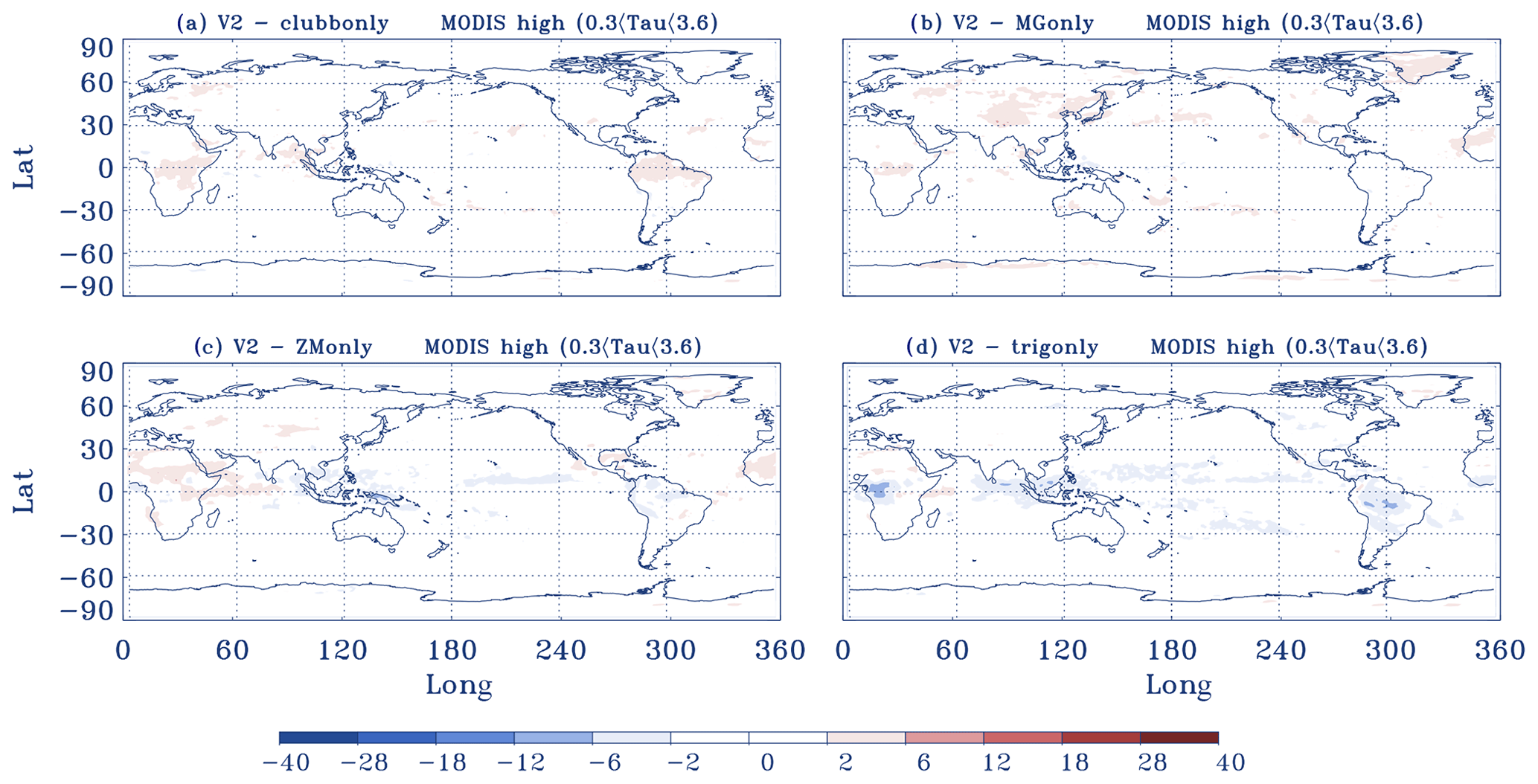
Figure A4 Difference in optically thin high-cloud fraction from the MODIS simulator (0.3< Tau <3.6) between sensitivity tests and the default E3SMv2 run. (a) E3SMv2 with CLUBB-related parameters changed from v2 to v1, (b) E3SMv2 with MG2-related parameters changed from v2 to v1, (c) E3SMv2 with ZM-related parameters changed from v2 to v1, and (d) E3SMv2 with the dCAPE_ULL trigger turned off. All results are from 6-year AMIP-style climatology runs.

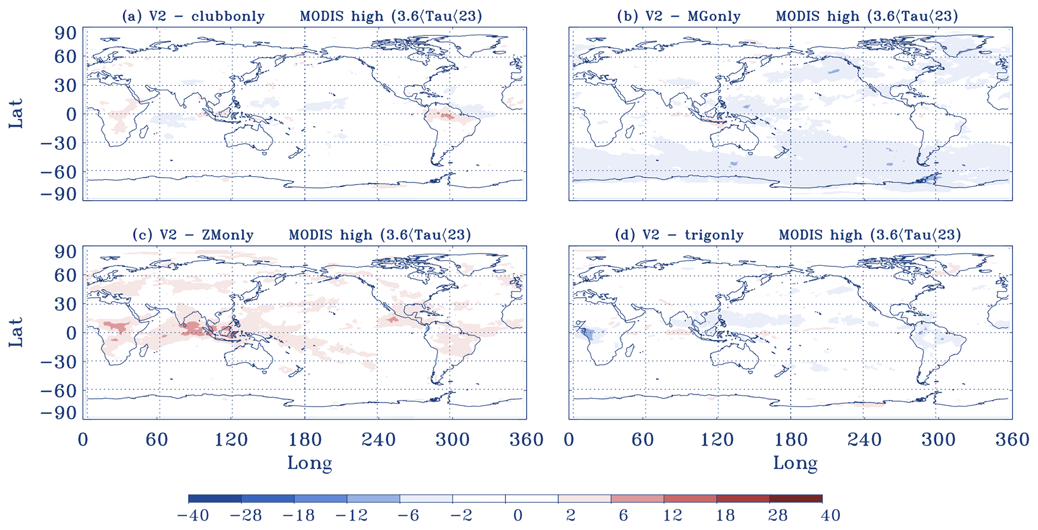
Figure A5 Difference in optically intermediate high-cloud fraction from the MODIS simulator (3.6< Tau <23) between sensitivity tests and the default E3SMv2 run. (a) E3SMv2 with CLUBB-related parameters changed from v2 to v1, (b) E3SMv2 with MG2-related parameters changed from v2 to v1, (c) E3SMv2 with ZM-related parameters changed from v2 to v1, and (d) E3SMv2 with the dCAPE_ULL trigger turned off. All results are from 6-year AMIP-style climatology runs.

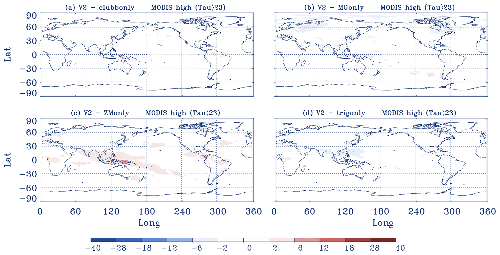
Figure A6 Difference in optically thick high-cloud fraction from the MODIS simulator (Tau >23) between sensitivity tests and the default E3SMv2 run. (a) E3SMv2 with CLUBB-related parameters changed from v2 to v1, (b) E3SMv2 with MG2-related parameters changed from v2 to v1, (c) E3SMv2 with ZM-related parameters changed from v2 to v1, and (d) E3SMv2 with the dCAPE_ULL trigger turned off. All results are from 6-year AMIP-style climatology runs.