the Creative Commons Attribution 4.0 License.
the Creative Commons Attribution 4.0 License.
 | 26 Feb 2024
Flux coupling approach on an exchange grid for the IOW Earth System Model (version 1.04.00) of the Baltic Sea region
Sven Karsten
Hagen Radtke
Matthias Gröger
Ha T. M. Ho-Hagemann
Hossein Mashayekh
Thomas Neumann
H. E. Markus Meier
In this article the development of a high-resolution Earth System Model (ESM) for the Baltic Sea region is described. In contrast to conventional coupling approaches, the presented model features an additional (technical) component, the flux calculator, which calculates fluxes between the model components on a common exchange grid. This approach naturally ensures conservation of exchanged quantities, a locally consistent treatment of the fluxes, and facilitates interchanging model components in a straightforward manner. The main purpose of this model is to downscale global reanalysis or climate model data to the Baltic Sea region as typically, global model grids are too coarse to resolve the region of interest sufficiently. The regional ESM consists of the Modular Ocean Model 5 (MOM5) for the ocean and the COSMO model in CLimate Mode (CCLM, version 5.0_clm3) for the atmosphere. The bi-directional ocean–atmosphere coupling allows for a realistic air–sea feedback that outperforms the traditional approach of using uncoupled standalone models, as typically pursued with the EURO-CORDEX protocol. In order to address marine environmental problems (e.g., eutrophication and oxygen depletion), the ocean model is internally coupled with the marine biogeochemistry model, ERGOM, set up for the Baltic Sea's hydrographic conditions. The regional ESM can be used for various scientific questions such as climate sensitivity experiments, reconstruction of ocean dynamics, study of past climates, and natural variability, as well as investigation of ocean–atmosphere interactions. Therefore, it can serve for a better understanding of natural processes via attribution experiments that relate observed changes to mechanistic causes.
- Article
(4791 KB) - Full-text XML
- BibTeX
- EndNote


The European continent and its marginal seas are located between the polar climate zone in the north and the subtropical climate in the south and are likewise influenced by a temperate maritime climate in the west and a continental climate with high seasonal amplitudes in the east. Consequently, the climate of Europe is highly variable, resulting in many different climate zones to be distinguished (Köppen and Geiger, 1930). These circumstances make this region a challenge for the development of coupled ESMs (Gröger et al., 2021). This is in particular the case for the Baltic Sea region, which is known for its high natural variability, complicated coast lines given by numerous islands, narrow channels between the basins, and the small baroclinic Rossby radius (Fennel et al., 1991), resulting from a permanent haline stratification.
Thus, simulating the Baltic Sea's regional climate requires a sufficiently high spatial resolution of the oceanic model grid. However, the corresponding atmospheric circulation is usually simulated on a much larger domain, as the pathways of cyclones originating from the North Atlantic region should be part of it. For this reason, the atmospheric model cannot be discretized with the same high resolution as the ocean model at reasonable numerical costs. Hence, an adequate strategy is needed to provide the highly resolved oceanic information to a suitable atmospheric model simulating the Baltic Sea's regional climate.
For the recent past, appropriate measurement data (or derived products such as satellite data) for the Baltic Sea's surface variables are available that may serve as the lower boundary for the atmospheric model. This enables uncoupled simulations where the atmosphere is simulated first, using observed values for the ocean state, and then an ocean model can later be driven with the atmospheric variables as forcing. This strategy, however, naturally fails for future projections. Projections for the Earth's future climate are based on global ESMs, i.e., platforms that interactively couple different components of the Earth system (e.g., atmosphere, biosphere, cryosphere, ocean, e.g., Heinze et al., 2019). Still, the resolution of these models is insufficient to explicitly resolve important small-scale processes (e.g., land–sea mask effects, polar lows, etc.) leading to, for example, unrealistic wind fields over the Baltic Sea (Meier et al., 2011). Therefore, regional models were developed that represent a step forward to more sophistically include small-scale processes and more realistically represent orography. However, most of these models for the Northern European region consist only of a single standalone model for the atmosphere that is driven by input data either from global models or from reanalysis products at the model boundaries. For future projections, this approach is problematic, as input information can only be derived from global models that can have substantial biases in the region of interest (especially in coastal regions, where the coarse resolution of the land–sea mask can become insufficient). Although numerous tested methods exist to bias-correct model forcing data for the historical period (e.g., Teutschbein and Seibert, 2012; Vaittinada Ayar et al., 2021), their application for future periods cannot be validated and may therefore be problematic. In addition, these models employ bulk formulas for the exchanged fluxes with rather simplistic models for the transfer coefficients. This argues in favor of the development of fully coupled Regional Earth System Models (RESMs) for future projections that consistently account for the local peculiarities of the considered domain (Gröger et al., 2021).
For the Baltic Sea, two independent coupled model systems from the Danish Meteorological Institute and the Swedish Meteorological and Hydrological Institute demonstrated an improvement of simulated winter Sea Surface Temperatures (SSTs) compared with their corresponding ocean-only simulations (Tian et al., 2013; Gröger et al., 2015). However, the fluxes are calculated entirely by the atmospheric model on its coarser grid.
In contrast to the existing RESMs for the Baltic Sea region, the IOW ESM presented here involves a third component, called the flux calculator, that computes the fluxes on an exchange grid formed by the intersections between the two model grids. This approach naturally ensures locally consistent treatment of the fluxes and conservation of exchanged quantities. Thus, the drawbacks accompanying the high resolution of the oceanic model grid and the large atmospheric simulation domain can be circumvented. Moreover, this approach enables more flexibility in interchanging model components and thus simplifies the development. At the present stage the IOW ESM consists of the MOM5 model (Neumann et al., 2021) for the Baltic Sea and the CCLM model (version 5.0_clm3) (Steger and Bucchignani, 2020) for the atmosphere on the EURO-CORDEX domain.
The exchange grid method is not new but was introduced by Balaji et al. (2006) for the Flexible Modeling System of the Geophysical Fluid Dynamics Laboratory at Princeton University. Also, the coupler Earth System Modelling Framework with the National Unified Operational Prediction (ESMF/NUOPC) follows this philosophy, where a mediator component can be used as an equivalent to our flux calculator, and the exchange grid calculation is performed on-the-fly during the model runtime (Campbell and Whitcomb, 2013). From the global modeling perspective the National Center of Atmospheric Research (NCAR) Community Earth System Model (CESM) (Danabasoglu et al., 2020) follows a similar strategy of consistently calculating fluxes by an additional component corresponding to the presented flux calculator. An alternative approach to conservative mapping was introduced by Furevik et al. (2003), where the action of an exchange grid was mimicked by a stochastic sampling in the fashion of a Monte Carlo simulation. However, for the Baltic Sea area, our model system is, to the best of our knowledge, the first to fully employ this approach. The ICONGETM coupled model system (Bauer et al., 2021) used an ESMF/NUOPC exchange grid before, but only for the conservative mapping of fluxes, the flux calculations were still performed by the atmospheric model component on its own grid, not by the mediator.
The paper is structured as follows. First, the theoretical background and the methodology of the developed coupling approach is described in Sect. 2, including implementation details. In order to investigate the differences between the chosen exchange grid and the more traditional coupling strategies, reference runs for different types of exchange grids with ERA5 (Hersbach et al., 2019) reanalysis data as atmospheric boundaries have been performed and are compared and discussed in Sect. 3. The focus of this article is on the flexibility in model development, the consistency of the presented flux calculation, and the facilitation of running simulations as well as performing subsequent data analysis that is enabled by the presented framework. Still, the presented simulations have been performed with realistic setups for the model components for several decades and thus give a robust impression of the model performance. Finally, the work is concluded in Sect. 4 and further details can be found in the Appendix.
One basic problem when dealing with RESMs is that the individual components (atmosphere, ocean, land, etc.) are described by different models that act on different grids (see Figs. 1 and 2).
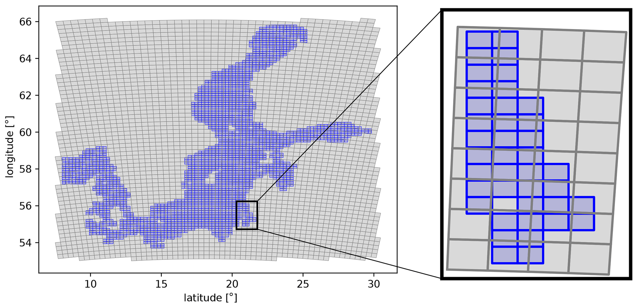
Figure 1Overlaying grids of atmospheric and ocean models for the Baltic Sea.
Still, the components have to be coupled in order to communicate their state to each other and exchange fluxes as in reality.
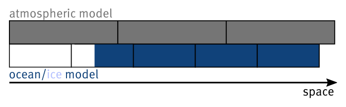
Figure 2Schematic of atmosphere and ocean model grids. The bottom model can support different surface types, for instance, water (blue) and ice (white). However, both are typically represented by the same grid cell and only the concentration of each surface type in that grid cell is considered. In the illustrated case, the first left ocean model grid cell has an ice concentration of 100 % and the second left has roughly 40 % ice and 60 % liquid water, whereas all other cells are fully covered with water.
2.1 The exchange grid and the flux calculator
In the standard approach to coupling climate model components, the exchanged fluxes are calculated in the atmospheric model (Wang et al., 2015; Sein et al., 2015). As fluxes naturally depend on the state of the ocean, the corresponding information has to be communicated to the atmosphere first. Owing to the normally lower resolution of the atmospheric grid, information on the ocean's state has to be averaged (weighted by areas) over several ocean grid cells and typically over different surface types (water, different ice classes or land; see blue and white boxes in Fig. 2 and for more details Fig. B1 in Appendix B).
With the averaged state information from the ocean model (ice or land model) and its own internal state, the flux can be calculated (as a field on the atmospheric grid) by the atmospheric model.
Subsequently, the flux field has to be redistributed on the ocean (sea-ice or land) cells (again in a area-weighted manner such that the exchanged quantity is overall conserved, i.e., a conservative mapping; see Fig. B1b). As the flux is only calculated from averaged information, this approach is locally not consistent and can become inaccurate. This is especially true if many bottom grid cells are covered by one atmospheric grid cell.
The alternative approach chosen within the developed ESM is the introduction of a third component, i.e., the flux calculator that acts on an exchange grid. The most natural choice for such an exchange grid would be the set of intersections between the atmospheric and the ocean grid cells. This grid has, by construction, a higher resolution than all involved model components (see Fig. 3).
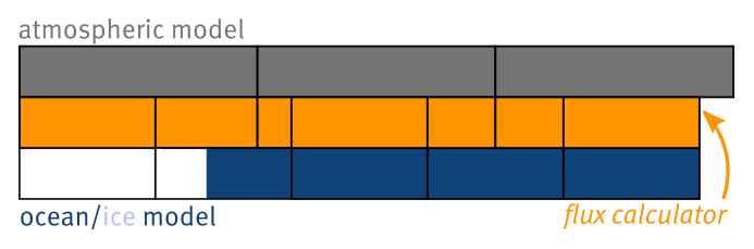
Figure 3Introduction of the exchange grid (orange boxes) on which the flux calculator is acting.
Thus, the exchange grid is capable of resolving all peculiarities covered by the involved model grids.
Employing the aforementioned exchange grid, the example from above, i.e., fluxes shall be communicated between the atmosphere and the ocean, is then treated as follows. First, the model components of the coupled model send their necessary state variables to the flux calculator. The variables are thereby mapped onto the exchange grid (see Fig. 4a), via conservative mapping. Importantly, as the intersection exchange-grid cells are always smaller or equal to the grid cells of the models, this mapping does not feature any averaging and, thus, no information is lost. Moreover, different surface types can be treated individually as this information on features of the ocean, sea-ice or land model can be implemented in the flux calculator.
Second, with all the state information, the flux calculator is then able to calculate the flux of interest. Any formula can be used that derives the desired fluxes from the available state variables. The calculation only requires local information and can be surface-type-dependent. The resulting flux has to be finally mapped onto the bottom grid (see Fig. 4b), again via conservative mapping. Note that, although not shown in the figures (for the sake of clarity), the exact same fluxes are communicated to the atmospheric model as well. This ensures a conservative and locally consistent exchange of mass, energy, and momentum between the different model components.
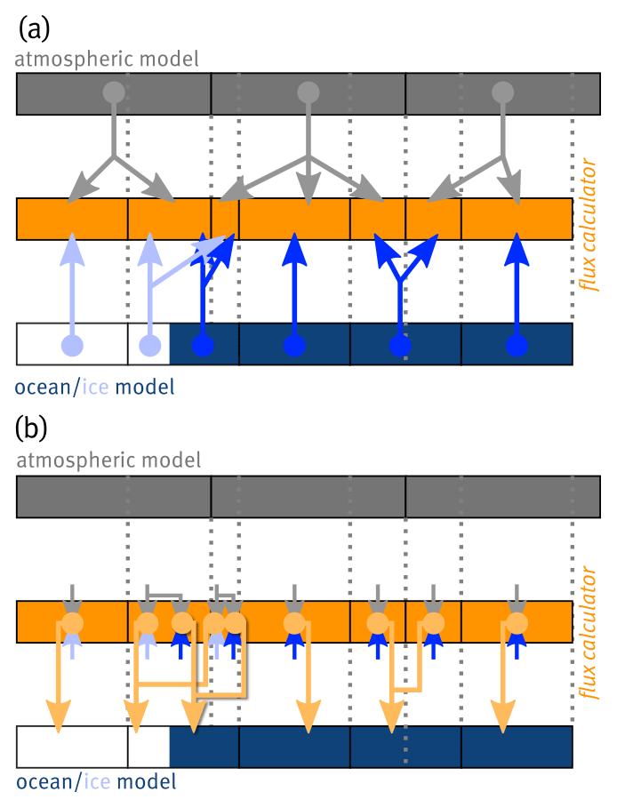
Figure 4Coupling the models via the exchange grid and the flux calculator. (a) State variables, calculated in the respective models (marked by the filled circles), are communicated to the flux calculator (as visualized by the arrows) without averaging. (b) Fluxes are calculated on the exchange grid and subsequently communicated to the bottom model.
However, the calculation of some fluxes does not depend only on surface fields and therefore are out of scope of the flux calculator capabilities. In particular, precipitation and (downward shortwave and longwave) radiative fluxes are calculated entirely by the atmospheric model and the resulting fluxes are sent via the flux calculator to the ocean model. Nevertheless, there is no direct communication between the two model components and this ultimately simplifies the interchangeability of the models. This is due to the fact, that either model can be exchanged (in principle) without affecting the source code of the other; only the self-developed flux calculator module has to be adapted.
In order to investigate the impact of the described exchange grid approach, two alternative exchange grid types are considered for comparison.
2.2 Different exchange grids
In Sect. 2.1, the described exchange grid is formed from the intersections of the involved models grids, henceforth called the intersection grid. The two apparent alternative exchange grids can then be either the atmospheric model grid or the ocean model grid itself.
As for a typical coupled model setup, the atmospheric grid has the lower resolution than the ocean model, the two resulting alternative exchange grids can differ quite substantially from each other, as well as from the intersection grid.
In any case, both alternatives will have (by construction) a lower resolution than the intersection-type exchange grid. With this more general conception of an exchange grid we are now able to consider three different kinds of coupling approaches on equal footing.
First, we consider the approach introduced in Sect. 2.1 and calculate fluxes by the flux calculator with state variables locally resolved on the intersection grid and subsequently communicate the fluxes to the models. Second and third, we may employ each of the model grids as the exchange grid and calculate fluxes with spatially averaged fields and then communicate the fluxes to the involved models. These two last cases also include the typical coupling approach, i.e., using a conservative mapping of state variables from the ocean to the atmospheric model accompanied by the flux calculation via the latter and the communication back to the former (e.g., Wang et al., 2015).
Importantly, the developed flux calculator methodology enables us to investigate all three approaches with the same infrastructure (i.e., the underlying source code). The only differences lie in the exchange grid and the resulting mapping matrices to and from the model grids. These different mappings are discussed in detail and visualized in the Appendix C. It can be seen from the figure therein that the differences between the intersection-type and ocean-model exchange grid are anticipated to be rather small (see Sect. 3.2, owing to the fact that many ocean grid cells are completely contained in a single atmospheric grid cell and therefore undergo the same flux calculations in both settings.
2.3 Implementation
As the first step, a working version of the coupled ESM is developed that consists of the MOM5 ocean model and the CCLM atmospheric model. Nevertheless, the ESM is designed in such a way that other models can be added and the current configuration could be extended or replaced by other suitable models in future. Technically, all components (including the flux calculator) communicate via the widespread OASIS3-MCT (version 4.0) coupling library (Valcke et al., 2013).
Note that since MOM5 and CCLM use time-independent horizontal grids, the exchange grid and all corresponding mapping matrices can be determined once in advance to the model run.
Furthermore, the exchange grid is only defined within the coupled region, i.e., the Baltic Sea.
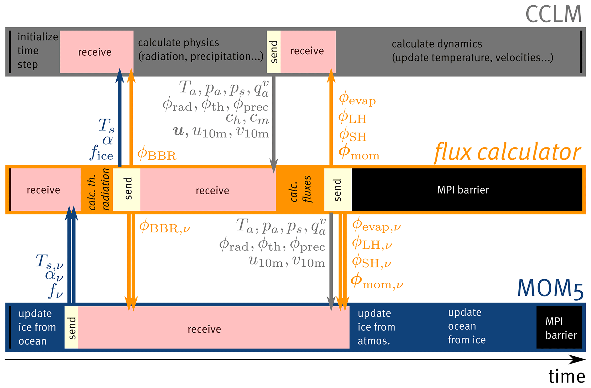
Figure 5Schematic sequence diagram for one coupling time step. The two model components, MOM5 and CCLM, are visualized as the blue and gray blocks respectively. The flux calculator is represented as the orange block. The calls of the coupling library routines are marked in light red for the blocking receiving function and in light yellow for the non-blocking send routine. Areas with the color corresponding to the particular model (blue and gray) mark the normal operation of the models. The simulation time runs from left to right. The scaling of the time axis is just illustrative and not quantitatively true. Arrows illustrate the data exchange of the spelled out quantities explained in Table 1, where double arrows stand for surface-type dependent fields, i.e., one communicated field for each surface type. The colors of the symbols represent the component from where they originate. For more detailed description see the main text.
2.3.1 Coupling cycle
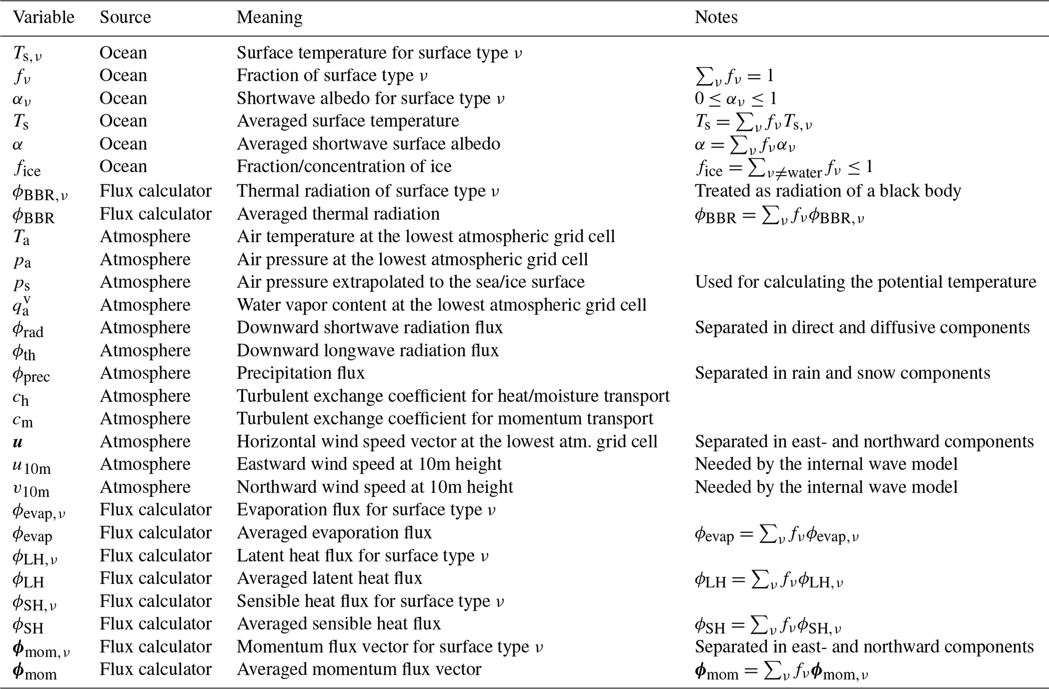
In the current implementation, the oceanic and atmospheric model exchange the following quantities via the flux calculator during one coupling time step (see also Fig. 5) and for more information on the exchanged variables, see Table 1. Note that all exchanged fields are taken instantaneously from the model components and sent to the flux calculator. Currently, no time averaging over a coupling cycle is employed; however, in future work, the impact of such an averaging might be considered.
In the beginning of each time step all components have to pass a global barrier, implemented with the Message Passing Interface (MPI) library (Message Passing Interface Forum, 2021), depicted by black vertical bars on the left of the figure. After all components passed the barrier and are thus synchronized, the ocean model starts with updating the internal ice model with the current state information of the underlying water body, whereas the flux calculator remains in the blocking receive function of the coupling library. In parallel, the atmospheric model does the necessary initialization of the time step until it calls the blocking receive function as well. As soon as the ice model is updated, the ocean model sends its state variables, i.e., surface temperature Ts,ν, the albedo αν, and the fraction or concentration fν of each surface type ν (water and five different ice classes categorized by their thickness; depicted by double arrows in Fig. 5) from each grid cell to the flux calculator. After the send routine returns, the ocean model is waiting for input to update its ice model from the top. In the meantime, the sent fields are mapped from the ocean model's grid to the exchange grid and then passed to the flux calculator. With this input, the flux calculator can compute the black-body (thermal) radiation that is emitted by the ocean (see Sect. 2.3.2). This quantity is then sent to both models (and mapped to their grids) where it is added to the atmospheric thermal radiation budget and subtracted from the ocean's one. Note that the thermal radiation that is emitted by the atmosphere is entirely computed in the atmospheric model as it is not simply given as black-body radiation (but also depends on cloudiness and the water vapor in layers above the surface). As the atmospheric model also requires the ocean's state variables mentioned above (for computing transfer coefficients, radiation fluxes and precipitation), they are passed through the flux calculator to the atmospheric model. However, owing to the fact that the atmospheric model does not distinguish surface categories, these variables are averaged over different surface types, e.g., (see Table 1). By sending these averaged variables from the CCLM to the flux calculator, it is implicitly assumed that above the surface of variable temperature, the atmosphere is homogeneous on the scale of the model grid box, from the first level of the model to the top. This assumption may not be valid in grid boxes with large temperature gradients, such as those that are partially covered with sea ice. However, it has been a common approach in the state-of-the-art Earth system models that the atmospheric model component does not treat the surface types separately. Different fluxes over open ocean and sea ice may be accounted for if the effect of these different surface types is considered separately throughout the atmospheric column, such as it is the case in the new ICOsahedral Nonhydrostatic (ICON) weather and climate model (Zängl et al., 2015).
After the send function has finished, the flux calculator is waiting for more input from the atmospheric model to calculate the other fluxes. During the blocking of the flux calculator and the ocean model, the atmospheric model can update its physics, i.e., calculating radiation fluxes, precipitation and transfer coefficients, for instance. The resulting fields are then sent to the flux calculator, which is released from the blocking receive function, whereas the atmospheric model is now waiting for the lower boundary surface fluxes. With the transfer coefficients over the coupled domain (i.e., the Baltic Sea) and the state variables from both model components, the flux calculator can calculate the evaporation, latent and sensible heat, as well as momentum fluxes (see Sect. 2.3.2). All quantities are computed on the exchange grid and sent to both models, which can then perform their final updating of the remaining variables with the given surface boundary fluxes. As soon as a component has reached the end of the current time step it is blocked by the MPI barrier before beginning the next cycle. Importantly, calculations in the flux calculator as well as the communication are restricted to grid cells that are coupled, i.e., grid cells that intersect with the ocean model's horizontal grid at the Baltic Sea surface.
In the case of the intersection-type exchange grid, the conservation of mass, energy, and momentum is naturally ensured in the coupled system. Radiation and precipitation fluxes that are not computed by the flux calculator, are simply passed through to the ocean model. The downward radiation fluxes are then redistributed by the MOM5 model to different surface types, resulting in different net fluxes depending on the particular surface albedo (Sect. 2.3.2). Additionally, the ocean model requires a few atmospheric state variables, i.e., atmospheric pressure and 10 m wind-speed components for the sea-ice, the turbulence, and the wave model that are implemented in the MOM5 component.
2.3.2 Flux formulas
The formulas used to calculate the exchanged fluxes are based on the corresponding CCLM (Doms et al., 2013) implementation. This implementation is in turn derived from the work of Louis (1979), which is briefly summarized in the following.
Central ingredients of the flux calculation are the air's density over the specific surface type ν (see also Appendix D) and the horizontal wind velocity from the lowest atmospheric grid cells. The coefficients for turbulent moisture and heat transfer as well as for the turbulent momentum transfer are obtained from the CCLM model via the Monin–Obukhov similarity theory (Monin and Obukhov, 1954). As these coefficients are calculated on the coarser atmospheric grid, they only account for the average sea-ice fraction of the underlying ocean grid cells instead of being decomposed into coefficients over ice and water, which can be very different. Hence, and are insensitive to the different scales of the surface heterogeneity, i.e., an ice front separating an ice-covered area from an area of open water (large-scale heterogeneity) is treated in the same way as ice fractured by leads (small-scale heterogeneity). Nevertheless, the presented formulas can be considered a step forward to improve on this deficiency, as they take different surface categories (water and ice) into account for variables other than the transfer coefficients that enter the flux calculation.
The evaporation mass flux is calculated assuming that the air adjusts its water vapor content to the one present at the sea/ice surface , i.e.,
where all quantities are meant to be functions of , i.e., the horizontal location on the sea surface and time; however, for the sake of brevity, we skip these arguments. How the surface-type-dependent water vapor content is calculated by the flux calculator is shown in Appendix D2.
The latent heat flux is then directly proportional to the evaporation
where ΔHν is the constant for the latent heat consumed/released by evaporation, freezing, or sublimation, depending on the type of phase transition related to the individual surface types.
The sensible heat flux is determined by the difference between the temperatures of the lowest (discretized) atmospheric layer and the surface , i.e.,
The appearing (where Rd is the gas constant for air) is the atmospheric potential temperature directly at the surface and Cp is the air's heat capacity at constant pressure.
The momentum fluxes (i.e., the shear stress at the components' interface) in x and y direction depend nonlinearly on the wind velocity at the lowest atmospheric layer and are calculated as
It is noteworthy, that in the current setup for the Baltic Sea tides are not considered and thus the horizontal velocity components of the ocean's surface ( to 10−1 m s−1) are negligible compared with the atmospheric ones (∝1…10 m s−1) and are thus omitted.
The thermal radiation that is emitted in an upward direction by the ocean is described by the radiation of a black body having the ocean's surface temperature, i.e., long-wave albedo is neglected. Thus, the thermal flux can be calculated via the Stefan–Boltzmann law suitable for black-body radiation
where σ is the Stefan–Boltzmann constant. Importantly, as the thermal radiation depends strongly nonlinearly on the temperature, this flux exemplifies the importance of the local consistency within the coupling. In other words, the averaged flux can differ strongly from the flux calculated with the averaged temperature , where the latter would correspond to the flux calculated by the atmospheric model.
As stated above, the downward radiation fluxes (i.e., short-wave and long-wave radiation) do not depend only on surface fields; they are thus entirely calculated by the atmospheric CCLM model and then passed through the flux calculator to the ocean model. The ocean model can then use its information on the different albedos of different surface categories ν to distribute the net flux (without the reflected part) onto the individual surface constituents as
The atmospheric model, on the other hand, receives the averaged albedo via the flux calculator from the ocean/ice model as
With this averaged albedo the atmospheric model calculates its own net radiation flux from the downward flux as
Although being calculated differently by the two models, it is shown in Appendix D that the resulting net fluxes are equal (when averaging over the contributing surface types in the ocean model grid cell).
Note that all the presented formulas for fluxes might be changed, e.g., to involve different methods, within the flux calculator source code without further changing the model codes. Thus, the presented approach, using an external component for the flux calculation, greatly facilitates sensitivity experiments with respect to surface boundary fluxes. It should be stressed, however, that in order to further improve on the sensitivity of the transfer coefficients with respect to different surface types, the calculation of and should be implemented in the flux calculator itself, which is currently out of scope. Alternatively, the employed atmospheric model should be able to treat different surface categories separately and to send the respective fields to the flux calculator.
2.4 Simulation setup
The following test setup has been used to perform benchmark simulations. In advance, ERA5 reanalysis data have been prepared as forcing/boundary data for the CCLM atmospheric model for the time period of 1 January 1959 to 31 December 1999. The forcing/boundary data have been processed using the COSMO pre-processing tool int2lm (Schättler and Blahak, 2013), which performs the interpolation from the coarse resolution ERA5 data to the employed resolution of the CCLM. With these data the coupled CCLM is forced over the EURO-CORDEX (Jacob et al., 2014) domain using a resolution of 0.22° by 0.22° and parameters similar to the setup used in (Ho-Hagemann et al., 2017, 2020). The coupled MOM5 simulates the Baltic Sea model with a horizontal resolution of 3×3 nautical miles. At the open boundary to the North Sea, we use climatologies for all prognostic model variables. The sea level elevation is estimated from the wind field by a statistical approach and the river runoff and nutrient loads are derived from HELCOM compilations (Neumann et al., 2021). The marine bio-geochemistry is modeled by the latest version of the internally coupled ERGOM (Neumann et al., 2021).
With this setup three runs are performed. First, the intersection-type exchange grid is used (Sect. 2.1). Second and third, the two model grids serve as the exchange grid respectively.
The runs are performed for a time span of 41 years, i.e., 1 January 1959 to 31 December 1999, where the first year 1959 is considered to be the spin-up phase. The model time steps are 600 and 150 s for the oceanic and atmospheric model respectively. In the atmosphere, radiation fluxes are updated every hour; the timestep for the physics is 150 s and is internally further subdivided to account for fast modes in the dynamics. The ocean model time step is 600 s and the time step of the coupling between the two models is also set to 600 s to temporally resolve strong wind gusts (Davis and Newstein, 1968). An investigation of the impact of different coupling time step sizes is planned for future work.
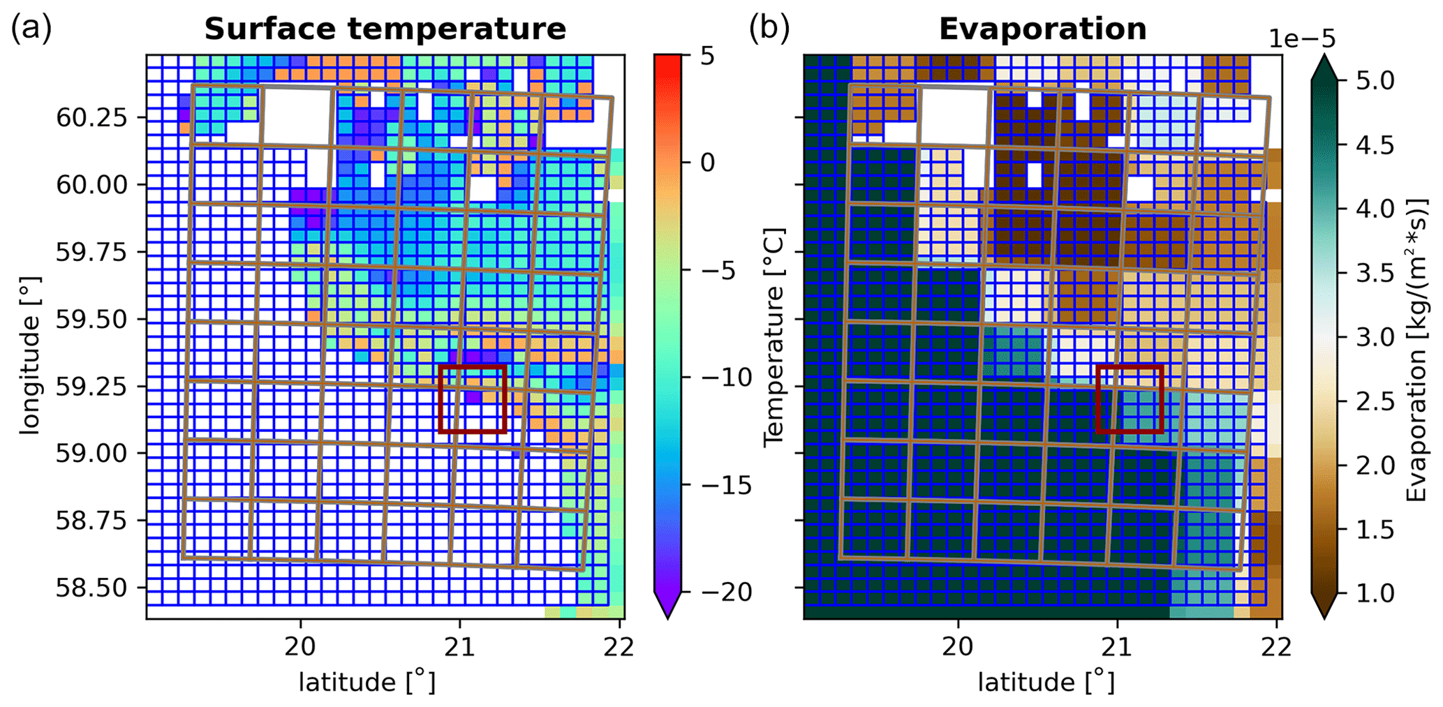
Figure 6Snapshots of the ocean's surface temperature (for ice-covered cells) and evaporation flux before the instability, i.e., 9 January 1960 south-east of the Åland island. (a) shows the surface temperature and the involved grids, i.e., blue boxes represent the ocean's grid and orange boxes the exchange grid, which is identical to the atmospheric grid. White ocean cells correspond to ice-free cells, which are omitted for the sake of clarity. White areas without boxes represent land. In (b) the evaporation instead of temperature is depicted. The dark red rectangle is centered around 21.08° E and 59.20° N (see text for further description).
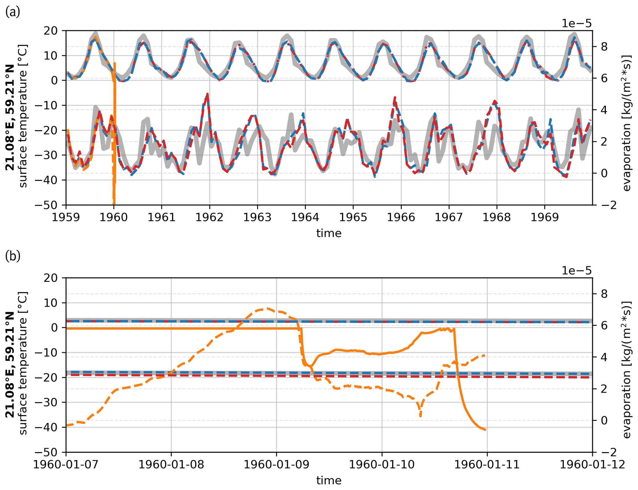
Figure 7Time series of the ocean's surface temperature and evaporation flux at 21.08° E and 59.20° N. The colors represent the different exchange grid types, where blue stands for the intersection grid, red for the ocean model's grid, and orange for the atmospheric grid. The light gray curves depict the ERA5 reference data. The upper curves in the upper panel (a) account for the surface temperature (left y-axis), whereas the lower curves represent the evaporation (right y-axis). The lower panel (b) shows the time evolution when the model using the atmospheric grid becomes instable. The solid orange curve shows the surface temperature (left y-axis) simulated with the atmospheric exchange grid. The dashed orange line depicts the corresponding evaporation flux (right y-axis).
3.1 Instability with the atmospheric exchange grid
When using the atmospheric grid as the exchange grid it was impossible to integrate the coupled model over the whole simulation time period. Instead, the model becomes instable after 12 months featuring an unrealistically low surface temperature at specific points on the ocean's grid. Figure 6 shows a snapshot on 9 January 1960, directly before the model stops. The cause of this instability is exemplified by considering the time evolution of temperature and evaporation for one specific location at 21.08° E and 59.20° N (centered in the dark red rectangle in Fig. 6), where the surface temperature falls below −40 °C within approximately 6 h (Fig. 7 and is magnified in panel (b) therein). It is evident that the evaporation has increased significantly before the surface temperature starts to vary strongly. Owing to the low exchange grid resolution (given by the atmospheric model), the evaporation's magnitude is mainly given by the surrounding ice-free cells (Fig. 6). Thus, the ice-covered cell is cooled down by the loss of latent heat, which is determined by the liquid water contained in the ice-free cells. Hence, the instability is a direct consequence of the inconsistency when calculating fluxes on the low-resolution atmospheric grid. Importantly, although the instability is explained with a very specific scenario, such inconsistencies may likely happen if the flux calculation is not consistent with respect to the spatial variation and surface-type dependence of the exchanged quantities.
In contrast, the surface temperature and evaporation rates simulated with the ocean-model exchange grid and the intersection-type exchange grid remain stable over the simulation time period. In Fig. 7 one can see that both model types simulate both quantities in good agreement with ERA5 reference data for 21.08° E and 59.2° N. Note that for the sake of clarity, only the 10 years plus spin-up time (1959) are depicted. A full analysis, including a final validation with respect to reliable reference data, is outside the scope of this study and will be performed separately in future publications. This would also include the investigation of a higher horizontal resolution of the atmospheric model grid in order to better resolve small call processes, e.g., cloud formation, and how these processes are influenced by the interactive coupling to the ocean variables, e.g., the spatially and time-dependent albedo.
3.2 Intersection grid vs. ocean model grid
As stated in Sect. 2.2, the differences between using the intersection grid and the ocean-model grid as the exchange grid are anticipated to be small. This also becomes apparent from Fig. 7 as the time series from both model types are almost identical. Thus, the mean difference in the seasonal SST data is not shown directly, as the differences are very small. Instead, in Fig. 8, the signal-to-noise ratio (SNR) of the differences between the SST from both model setups is depicted. The SNR is obtained from the time-averaged seasonal difference ΔSST between the two models divided by their common standard deviation , where σ1,2 are the individual standard deviations of the seasonal SST from both model runs.
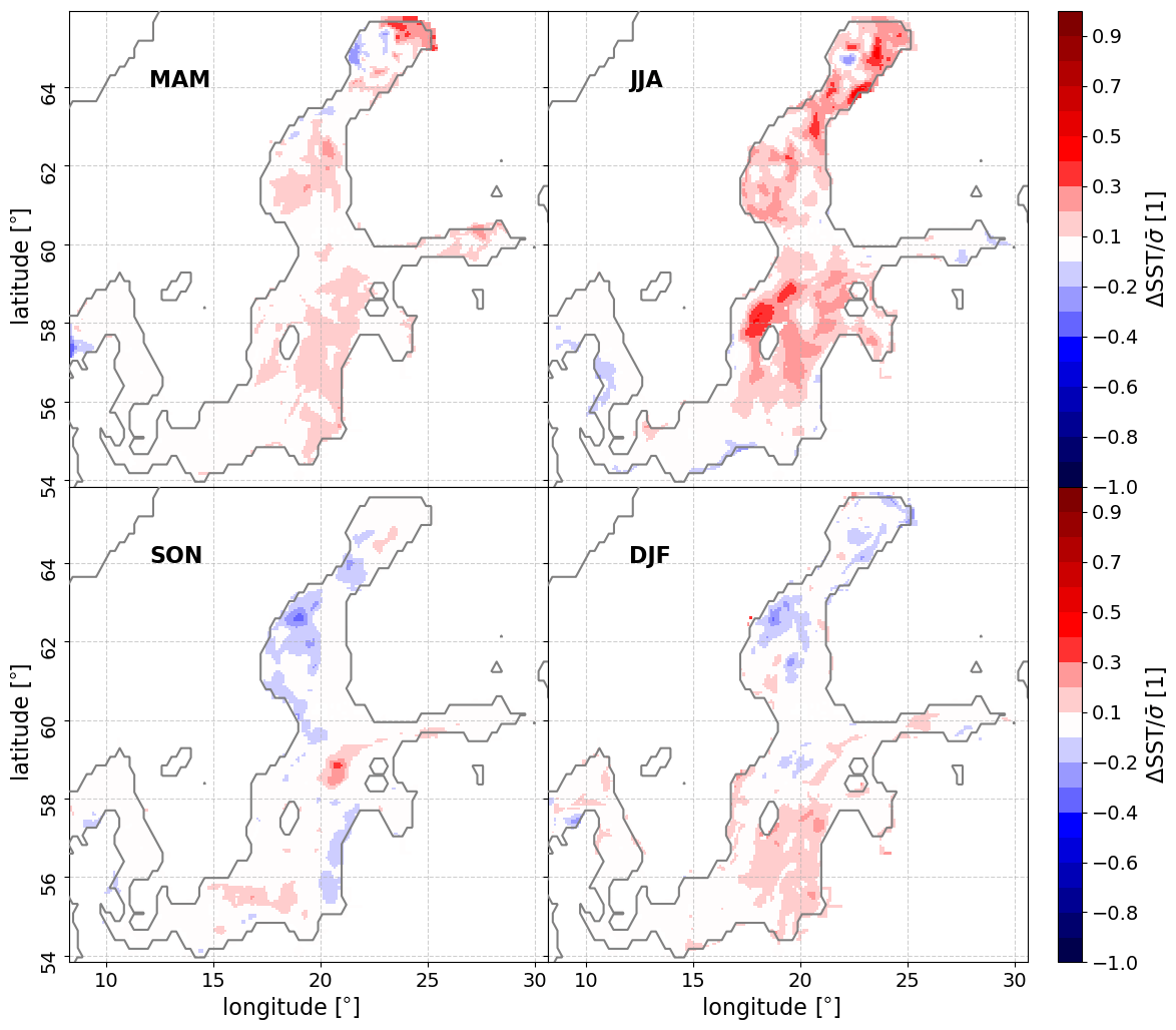
Figure 8SNR of differences between the temporal mean SST of the ocean-model grid and intersection-grid simulations. The maps show the time-averaged difference between the SSTs from the exchange-grid coupling simulation and the ocean-grid coupling simulation, divided by the standard deviation of the seasonal mean time series. The total evaluation period is 1 January 1960 to 31 December 1999. MAM: March, April, May (spring); JJA: June, July, August (summer); SON: September, October, November (fall); DJF: December, January, February (winter).
It can be seen from Fig. 8 that the mean signals do not differ significantly if one would take, for example, SNR ≥2 as a threshold. The largest SNR (>0.2) can be observed in the summer season around the Gotland island and in the Gulf of Bothnia, where the pattern that appears will be discussed below.
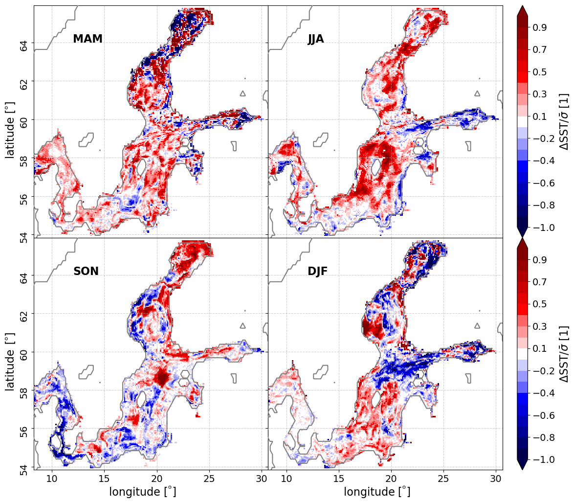
Figure 9SNR of differences between the ocean model's 95th percentile SST from ocean-model and intersection-grid simulations. See Fig. 8 for further description.
In contrast, when considering, for example, the differences in the 95th percentile calculated over the period 1 January 1960 to 31 December 1999, the deviations between the two exchange-grid types are more evident (see Fig. 9). In particular, the SNR for the summer features a similar pattern to that for the temporal mean (Fig. 8 second panel from the left) but with much higher values, even above one. The occurrence of this pattern, which is mainly concentrated around the Gotland island, might be explained to some extent by the different mappings when using different exchange grids (see Sect. 2.2) and in an extended discussion in the following paragraph. Moreover, for seasons where there is ice (i.e., spring and winter), one can see significant differences (with absolute values >1) in the Gulf of Bothnia. This might be due to surface-type-related inconsistencies as described in Sect. 3.1. We note that many assessments of climate extremes are based on thresholds in the higher percentile temperatures. Thus, the pronounced difference in the 95th percentile may indicate that the representation of such extremes will be sensitive to the choice of the exchange-grid. Hence, this may lead to systematic differences in the representation of extremes, such as marine heatwaves, which are commonly diagnosed through the 90th percentile SST (Hobday et al., 2016, 2018).
If so, one could expect that the intersection-type exchange grid yields more accurate results as it is by construction the most consistent approach. Using a coarser grid could systematically reduce extreme values since the averaging would yield spatially more homogenous fluxes, in line with what we see in the central Baltic Sea in spring, when the warming (by local shortwave radiation) is fastest. One has to keep in mind though that the simulated atmosphere-ocean systems can show chaotic behavior; thus, marginal differences in the beginning of the simulation may also increase to become random but substantial differences at later points of the simulation. An ensemble simulation with perturbed initial conditions would be needed to tell whether these differences in the representation of extremes are actually systematic.
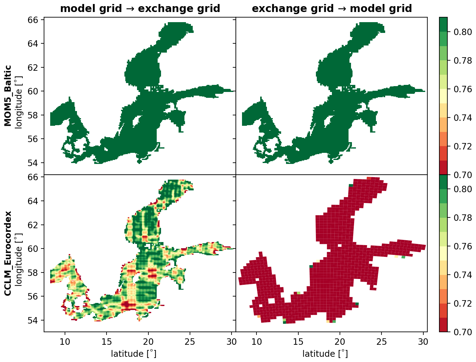
Figure 10Consistency map for flux calculation. Smoothed distribution of grid cell fractions that contribute to the flux calculation. A value of one means that only the grid cell itself contributes to the calculation of fluxes applied to that grid cell. A value smaller than one means that various surrounding cells contribute to the flux calculation.
In order to quantify the differences between the two exchange-grid types, a measure for the mapping consistency is needed. Such a measure can be found in the fraction of a grid cell that is involved for the calculation of the flux that is applied to the grid cell itself. If that fraction is exactly one, then the flux is calculated fully consistently, i.e., no averaging is performed. If the fraction is smaller, then other cells are also impacting the flux calculation, i.e., the information is averaged and fluxes may become inconsistent. In Fig. 10, the map of these fractions is depicted for the coupled domain when the ocean's model grid serves as the exchange grid. Note that the distribution of fractions is additionally convoluted with a Gaussian function to identify regions where more inconsistent flux calculation accumulates. This distribution is not isotropic as the involved model grids have different resolutions and are usually shifted with respect to each other. The resulting pattern can be considered as the superposition of two stationary waves with different wavelengths and phases yielding a beating between the two model grids (as can be seen in the lower left panel in Fig. 10).
In the case that the ocean model's grid is used as the exchange grid one has the following situation. First, the state information from both models (corresponding to the two rows in Fig. 10) is mapped to the exchange grid to calculate the fluxes (left panels therein). If the exchange grid is not the same as the model grid and is not the intersection grid, this mapping involves a loss of consistency, as the information has to be averaged over several grid cells of the source grid. In other words, the lower the number of these averaged-over cells, the higher the consistency. One can see that the mapping from the ocean to the exchange grid is (by construction) perfectly consistent in the whole coupling domain (upper left panel in Fig. 10). In contrast, when mapping from the atmospheric grid to the exchange grid, there are regions where more atmospheric grid cells contribute to the flux calculation, i.e., grid cells that are averaged over are more abundant. A significant part of these regions is located around the Gotland island and might be related to the pattern one can see in the significance of SST differences in Figs. 8 and 9. Importantly, when using the intersection grid as the exchange grid there is no inconsistency when mapping to it.
In the subsequent part of a coupling step (right panels in Fig. 10) the fluxes are mapped back to the model grids. Again the mapping from the exchange grid to the ocean grid is (by construction) perfectly consistent, whereas the mapping to the atmospheric model grid cells features high inconsistency, as the fluxes are averaged over a large number of exchange-(ocean-)grid cells. Nevertheless, this inconsistency when mapping from the exchange grid to the model grid cannot be avoided with all considered exchange grid types, see Appendix C.
The central focus of this article is to present a new regional ESM employing an exchange grid approach and to discuss the advantages and disadvantages. The model will be applied in dynamical downscaling experiments.
In contrast to existing coupled RESMs for the Baltic Sea, the presented coupling approach introduces an extra component that complements the involved circulation model components. This component called the flux calculator computes the fluxes between the models on an exchange grid, formed by the intersections of the model grids. That way, quantities can be exchanged locally consistently and their conservation within the coupled system is ensured. On top of the aforementioned intersection grid, other possible choices for the exchange grid are presented, i.e., taking one of the model grids as the exchange grid. Importantly, with the developed framework, these different choices can be investigated on the same footing without changing the setup of the involved models.
The current implementation of the coupled ESM consists of the MOM5 model for the Baltic Sea and the CCLM model for simulating the atmospheric dynamics over the EURO-CORDEX domain. The coupling cycle features the mapping of state variables from the models to the exchange grid and subsequent calculation of fluxes via well-known formulas introduced in Louis (1979) employing the Monin–Obukhov similarity theory (Monin and Obukhov, 1954) to obtain the transfer coefficients.
For each of the aforementioned exchange grid types an individual run of the coupled ESM has been performed with a realistic setup for both model components. If the atmospheric model provides the exchange grid, this leads to inconsistencies along borders that separate different surface types, e.g., water to ice or water to land. It turns out that this model configuration is not suitable for the considered setup without further modifications. In fact, the model becomes unstable in the second year of simulation as a result of an inconsistent evaporation flux applied to an ice-covered ocean grid cell located at the border to ice-free cells. This is because the evaporation is calculated on the coarse atmospheric model grid and thus accounts mainly for the neighboring ice-free cells. It is noteworthy that this deficit might be circumvented by updating the atmospheric model to CCLM version 6.0 or ultimately to the new ICON model (Zängl et al., 2015), which may both account for different surface types. The investigation of an updated configuration of the IOW ESM is reserved for future publications.
In contrast, the other two investigated exchange-grid types, i.e., the intersection grid and the ocean-model grid case, the model remains stable for the whole integration period 1 January 1959 to 31 December 1999. Both model variants yield seasonal mean SSTs that do not differ significantly. However, the 95th percentiles of the seasonal SST differ more strongly. The spatial distribution of these differences is related to a consistency map that reveals regions of inconsistent mapping between the involved grids, when using the oceanic exchange grid. In turn, using the intersection grid as the exchange grid naturally avoids these inconsistencies. Whether extreme events are differently described by the various coupling strategies will be investigated in future.
The presented methodology, employing the intersection grid as the natural choice for the exchange grid, provides a consistent treatment of the coupling in climate simulations. For the setup considered here, this approach outperforms the more standard method of calculating fluxes by the atmospheric model on its coarser grid. However, no significant improvements are apparent compared with the mean sea surface temperatures obtained with a flux calculation that is performed on the oceanic model grid. Whether the more significant differences in the 95th percentile SST would lead to an improved simulation of extremes is a topic for the next study. Still, the developed framework facilitates a flexible coupling between various components of the Earth system realized by different models. This opens the doorway to deducing robust dynamical downscaling experiments from global climate models to the climate of the Baltic Sea region.
| CCLM | COSMO model in CLimate Mode |
| CESM | Community Earth System Model |
| ESMF/NUOPC | Earth System Modelling Framework with the National Unified Operational Prediction |
| ESM | Earth System Model |
| ICON | ICOsahedral Nonhydrostatic |
| IOW | Leibniz Institute for Baltic Sea Research Warnemünde |
| MOM5 | Modular Ocean Model 5 |
| MPI | Message Passing Interface |
| NCAR | National Center of Atmospheric Research |
| RESM | Regional Earth System Model |
| SNR | Signal-to-Noise Ratio |
| SST | Sea Surface Temperature |
In contrast to Fig. 4 in the main text, Fig. B1 depicts how averaged quantities are used to calculate fluxes in the standard approach of coupling, i.e., fluxes are calculated by the atmospheric model.
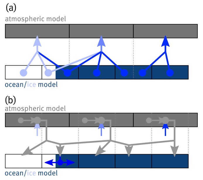
Figure B1The standard way of coupling. (a) Average of ocean's state variables communicated to the atmosphere. (b) Calculation of fluxes in the atmospheric model and remapping on to the ocean model grid.
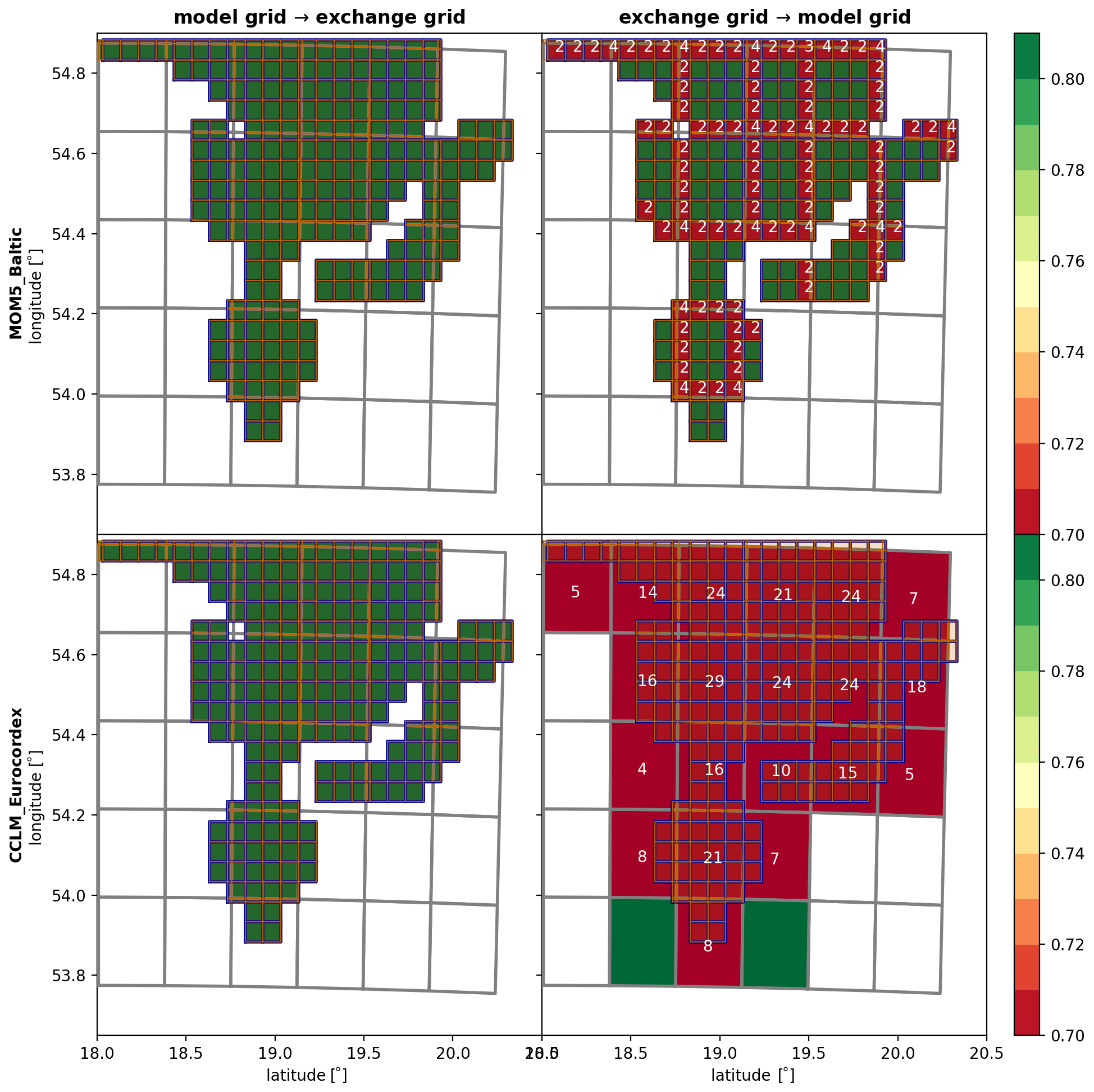
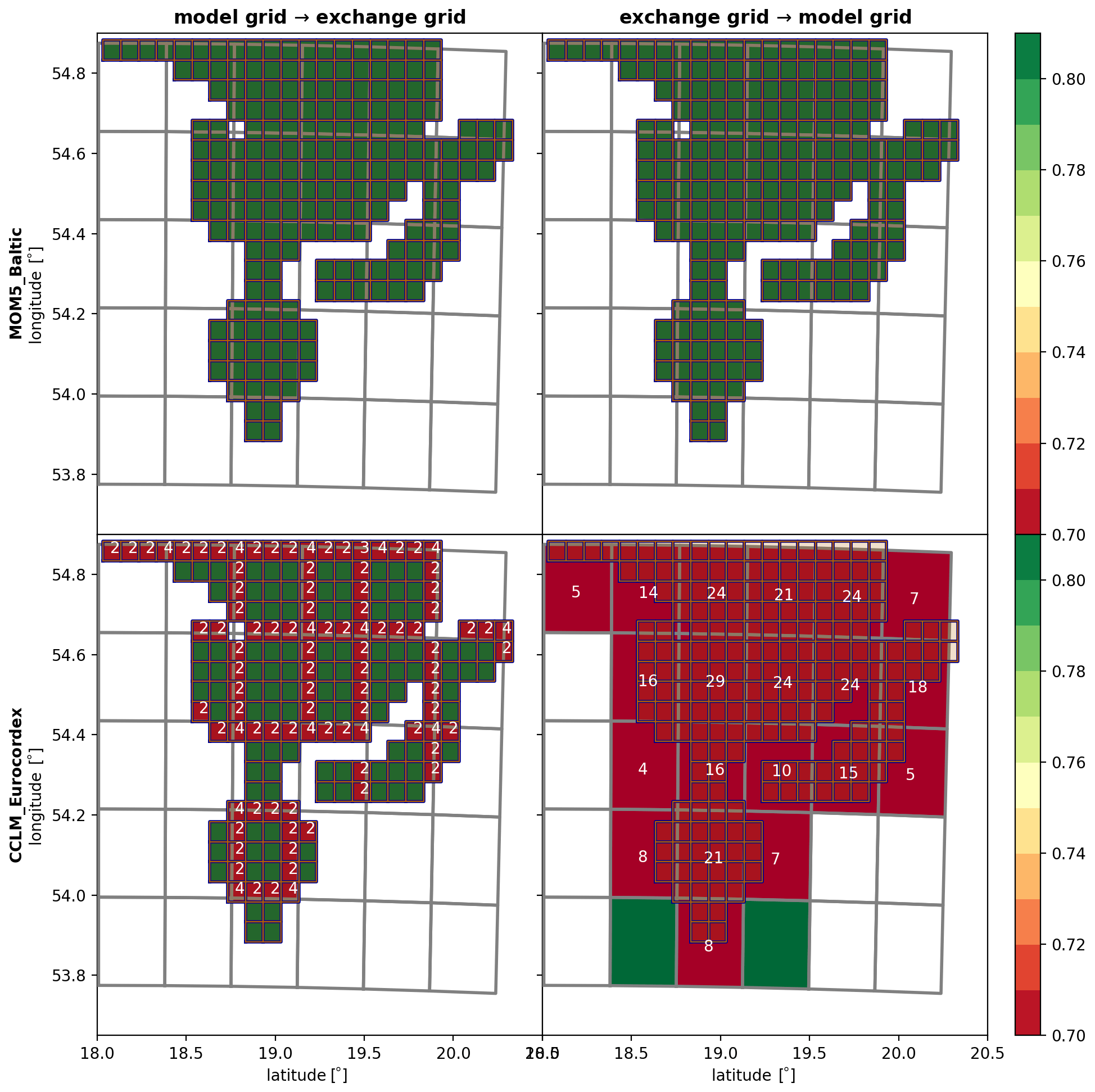
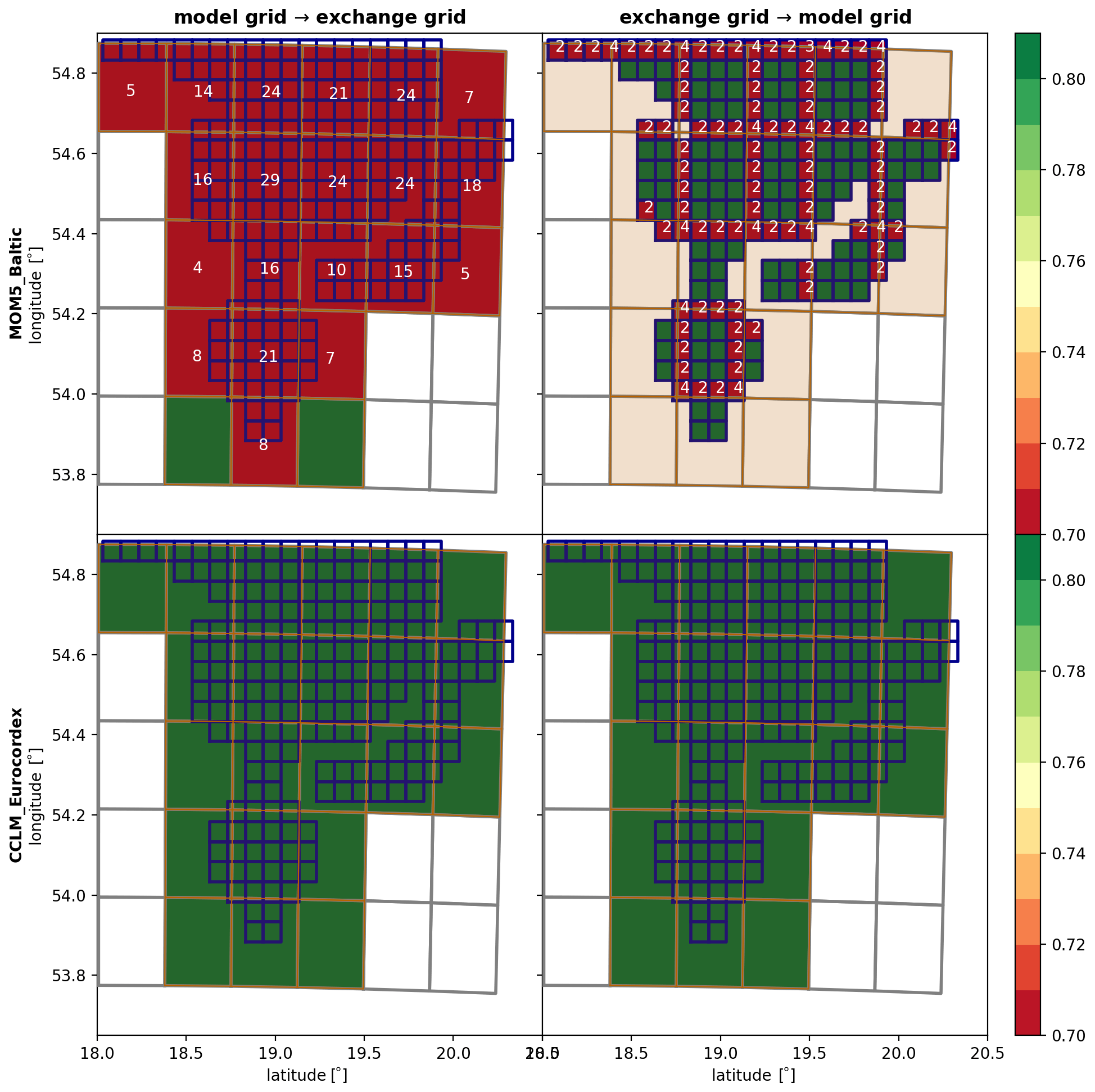
As stated in the main text in Sect. 2.2 the developed model framework enables comparison of different exchange grids on an equal footing. The difference between the various setups is discussed in detail in the following and visualized in Figs. C1, C2, and C3. The atmospheric grid is depicted by the gray lines, the ocean model's grid corresponds to the dark blue lines, and the exchange grid is shown by the thin orange lines. Exchange grid cells are additionally filled with transparent orange color. The opaque background colors refer to the mean mapping weight contributing to a particular cell on the destination grid. The white numbers show how many cells contribute to that mean. If no number is given, then only one cell contributes to the particular cell. The columns of each figure correspond to different phases during one coupling time step (from left to right). Left panels depict the sending of state variables from the models to the exchange grid; right panels show the communication of fluxes back to the models. The rows account for the two involved models.
The different mapping matrices for different exchange grids can be distinguished by the point in time when the spatial averaging is performed during the coupling cycle. For instance, in the case of the intersection grid, Fig. C1, the weights are all equal to one when the model's state variables are mapped to the exchange grid (see white grid cell areas in the left panels therein and note the color bar and figure caption). After the fluxes are calculated from the state variables, the fluxes have to be communicated back to the model grids. This mapping naturally involves averaging over several cells and cannot be avoided as the models do eventually feature different grids. This is illustrated by first the background color of the cells accounting for the mean mapping weight and second by the white numbers that count how many cells contribute to the particular destination grid cell. The higher this counter (and, thus, the lower the average mapping weight is) the more information is lost during the conservative mapping from one grid to the other. Importantly, when using the intersection grid as the exchange grid, the state variables are communicated to the flux calculator without any loss of information. Thus, no local inconsistency is due to any nonlinearity of the flux formulas and no errors stemming from the mapping procedure can be amplified by strongly nonlinear dependencies of the fluxes. Averaging over several cells only happens when the fluxes are finally communicated to the models.
In contrast, for the other two cases, there is a loss of information, when the state variables are communicated to the exchange grid for the flux calculation (see Figs. C2 and C3). The case when the ocean model's grid is used (see Fig. C2) seems to be quite similar to the intersection grid case. However, some local information is lost when mapping the atmospheric state variables to the exchange grid before the flux calculation. One can suppose from Fig. C3, that the largest local inconsistencies will occur when the standard approach is employed, i.e., the ocean's state variables are first communicated to the atmospheric grid, fluxes are calculated by the atmospheric model, and finally the fluxes are communicated back to the ocean. The impact of these inconsistencies is more quantitatively discussed in Sect. 3.1 and 3.2 in the main text.
D1 Ingredients of the flux calculation
Using the air pressure in the lowest atmospheric grid cells then the specific water vapor content over surface type ν can be calculated via
with the gas constants Rd for dry air and Rv for water vapor. The sea-surface temperature determines the saturation pressure that is calculated according to the Tetens approximation (Tetens, 1930) and the extension to temperatures below zero by Murray (1967), i.e.,
with Ts,ν in °C and where βν=17.27 if ν corresponds to water and βν=21.87 for ice. The temperature parameter Tν=237.30 °C for water and Tν=265.50 °C for ice.
Having the water vapor content at hand, one may then calculate the temperature at which dry air at the surface would show the same energy p⋅V as the moist air that is there now:
This temperature is related to the air's density by the ideal gas law (valid for dry air):
With the density all considered surfaces fluxes can be calculated as presented in the main text (Sect. 2.3.2).
D2 Calculating net radiation fluxes for different surface types
As was stated in the main text, the net radiation fluxes are calculated differently in the atmospheric and oceanic models. However, if we compare both net fluxes by taking the mean over the different surface types considered by the ocean model, we observe
Thus, the net fluxes calculated by both models are equal if we consider the mean flux applied to an ocean grid cell covered by different surface categories.
The source code of the IOW ESM (version 1.04.00) is available in multiple repositories collected in the Github organization https://github.com/iow-esm (last access: 27 July 2023). Frozen versions of the code repositories as used for this paper are archived on Zenodo. The main repository https://doi.org/10.5281/zenodo.8186789 (Karsten and Radtke, 2023a) is the entry point for the developed software framework and relates the repositories to each other. The sub-repositories are available as Zenodo archives and are listed in the description of the main product. Note that for the CCLM, there is only a patch available that contains the modifications implemented for the IOW ESM. In order to obtain the full model code, the original version of the CCLM code has to be downloaded. Further information can be found in https://github.com/iow-esm/components.cclm#readme (last access: 27 July 2023). The same holds for the preparation tool int2lm. Note that a complete version 1.01.00 of the coupled CCLM source code and version 1.00.02 of the int2lm tool has been made available to the editor and reviewers during the reviewing process of this manuscript.
A frozen version of the IOW ESM manual in jupyterbook format is archived on Zenodo https://doi.org/10.5281/zenodo.8186601 (Karsten and Radtke, 2023b). The current online version of the manual can be found at (last access: 27 July 2023).
A minimal setup to run the coupled model for a short period of time is stored on Zenodo https://doi.org/10.5281/zenodo.8167743 (Karsten, 2023).
The code, scripts, and manual of the IOW ESM in its current state have been developed by SK. HR designed the exchange grid approach including the flux calculator and implemented first prototypes of the coupling code and running scripts. In addition, HR guided the further development of the software framework. HTMH-H implemented a first version of the coupling interface to the CCLM. The setup for the CCLM was provided by HTMH-H and the setup for MOM5 was provided by TN. Atmospheric boundary condition generation was done by HM. HM also contributed to the discussions leading to a qualitative improvement of the model results. The coupled model simulations were performed, analyzed, and processed by SK. The manuscript text (including figures) has been prepared by SK and further iterated with the support of MG, HEMM, and all the other authors. HEMM designed and coordinated the research.
The contact author has declared that none of the authors has any competing interests.
Publisher’s note: Copernicus Publications remains neutral with regard to jurisdictional claims made in the text, published maps, institutional affiliations, or any other geographical representation in this paper. While Copernicus Publications makes every effort to include appropriate place names, the final responsibility lies with the authors.
The research presented in this study is part of the Baltic Earth program (Earth System Science for the Baltic Sea region, see http://www.baltic.earth, last access: 19 February 2024). HTMH-H acknowledges the German REKLIM project. The authors gratefully acknowledge the computing time granted by the Resource Allocation Board and provided on the supercomputers Lise and Emmy at NHR@ZIB and NHR@Göttingen as part of the NHR infrastructure. The calculations for this research were conducted with computing resources under the project mvk00050. The authors also thank Christian Steger, manager of the CLM community, for his help in publishing parts of the source code.
This research has been supported by the Federal Ministry of Education and Research (Bundesministerium für Bildung und Forschung, BMBF) through the project CoastalFutures (grant no. 03F0911E).
The publication of this article was funded by the Open Access Fund of the Leibniz Association.
This paper was edited by Sophie Valcke and reviewed by two anonymous referees.
Balaji, V., Anderson, J., Held, I., Winton, M., Durachta, J., Malyshev, S., and Stouffer, R. J.: The Exchange Grid: a mechanism for data exchange between Earth System components on independent grids, in: Parallel computational fluid dynamics 2005, 179–186, Elsevier, https://doi.org/10.1016/B978-044452206-1/50021-5, 2006. a
Bauer, T. P., Holtermann, P., Heinold, B., Radtke, H., Knoth, O., and Klingbeil, K.: ICONGETM v1.0 – flexible NUOPC-driven two-way coupling via ESMF exchange grids between the unstructured-grid atmosphere model ICON and the structured-grid coastal ocean model GETM, Geosci. Model Dev., 14, 4843–4863, https://doi.org/10.5194/gmd-14-4843-2021, 2021. a
Campbell, T. J. and Whitcomb, T. R.: Coupling Infrastructure and Interoperability Layer Extension Across All Earth System Components, Tech. rep., Defense Technical Information Center, Fort Belvoir, VA, https://doi.org/10.21236/ADA601269, 2013. a
Danabasoglu, G., Lamarque, J.-F., Bacmeister, J., Bailey, D., DuVivier, A., Edwards, J., Emmons, L., Fasullo, J., Garcia, R., Gettelman, A., Hannay, C., Holland, M. M., Large, W. G., Lauritzen, P. H., Lawrence, D. M., Lenaerts, J. T. M., Lindsay, K., Lipscomb, W. H., Mills, M. J., Neale, R., Oleson, K. W., Otto-Bliesner, B., Phillips, A. S., Sacks, W., Tilmes, S., van Kampenhout, L., Vertenstein, M., Bertini, A., Dennis, J., Deser, C., Fischer, C., Fox-Kemper, B., Kay, J. E., Kinnison, D., Kushner, P. J., Larson, M. V. E., Long, C., Mickelson, S., Moore, J. K., Nienhouse, E., Polvani, L., Rasch, P. J., and Strand, W. G.: The community earth system model version 2 (CESM2), J. Adv. Model. Earth Sy., 12, e2019MS001916, https://doi.org/10.1029/2019MS001916, 2020. a
Davis, F. K. and Newstein, H.: The variation of gust factors with mean wind speed and with height, J. Appl. Meteorol. Clim., 7, 372–378, 1968. a
Doms, G., Förstner, J., Heise, E., Herzog, H.-J., Mironov, D., Raschendorfer, M., Reinhardt, T., Ritter, B., Schrodin, R., Schulz, J.-P., and Vogel, G.: A description of the nonhydrostatic regional COSMO model. Part II: Physical parameterization, https://doi.org/10.5676/DWD_pub/nwv/cosmo-doc_5.00_II, 2013. a
Fennel, W., Seifert, T., and Kayser, B.: Rossby radii and phase speeds in the Baltic Sea, Cont. Shelf Res., 11, 23–36, 1991. a
Furevik, T., Bentsen, M., Drange, H., Kindem, I., Kvamstø, N. G., and Sorteberg, A.: Description and evaluation of the Bergen climate model: ARPEGE coupled with MICOM, Clim. Dynam., 21, 27–51, 2003. a
Gröger, M., Dieterich, C., Haapala, J., Ho-Hagemann, H. T. M., Hagemann, S., Jakacki, J., May, W., Meier, H. E. M., Miller, P. A., Rutgersson, A., and Wu, L.: Coupled regional Earth system modeling in the Baltic Sea region, Earth Syst. Dynam., 12, 939–973, https://doi.org/10.5194/esd-12-939-2021, 2021. a, b
Gröger, M., Dieterich, C., Meier, M. H. E., and Schimanke, S.: Thermal air–sea coupling in hindcast simulations for the North Sea and Baltic Sea on the NW European shelf, Tellus A, 67, 26911, https://doi.org/10.3402/tellusa.v67.26911, 2015. a
Heinze, C., Eyring, V., Friedlingstein, P., Jones, C., Balkanski, Y., Collins, W., Fichefet, T., Gao, S., Hall, A., Ivanova, D., Knorr, W., Knutti, R., Löw, A., Ponater, M., Schultz, M. G., Schulz, M., Siebesma, P., Teixeira, J., Tselioudis, G., and Vancoppenolle, M.: ESD Reviews: Climate feedbacks in the Earth system and prospects for their evaluation, Earth Syst. Dynam., 10, 379–452, https://doi.org/10.5194/esd-10-379-2019, 2019. a
Hersbach, H., Bell, B., Berrisford, P., Biavati, G., Horányi, A., Muñoz Sabater, J., Nicolas, J., Peubey, C., Radu, R., Rozum, I., Schepers, D., Simmons, A., Soci, C., Dee, D., and Thépaut, J.-N.: ERA5 monthly averaged data on single levels from 1959 to present, Copernicus Climate Change Service (C3S) Climate Data Store (CDS) [data set], https://doi.org/10.24381/cds.f17050d7, 2019. a
Ho-Hagemann, H. T. M., Gröger, M., Rockel, B., Zahn, M., Geyer, B., and Meier, H. M.: Effects of air-sea coupling over the North Sea and the Baltic Sea on simulated summer precipitation over Central Europe, Clim. Dynam., 49, 3851–3876, 2017. a
Ho-Hagemann, H. T. M., Hagemann, S., Grayek, S., Petrik, R., Rockel, B., Staneva, J., Feser, F., and Schrum, C.: Internal model variability of the regional coupled system model GCOAST-AHOI, Atmosphere, 11, 227, https://doi.org/10.3390/atmos11030227, 2020. a
Hobday, A. J., Alexander, L. V., Perkins, S. E., Smale, D. A., Straub, S. C., Oliver, E. C., Benthuysen, J. A., Burrows, M. T., Donat, M. G., Feng, M., Holbrook, J., Moore, P. J., Scannell, H. A., Sen Gupta, A., and Wernberg, T.: A hierarchical approach to defining marine heatwaves, Prog. Oceanogr., 141, 227–238, 2016. a
Hobday, A. J., Oliver, E. C., Gupta, A. S., Benthuysen, J. A., Burrows, M. T., Donat, M. G., Holbrook, N. J., Moore, P. J., Thomsen, M. S., Wernberg, T., and Smale, D. A.: Categorizing and naming marine heatwaves, Oceanography, 31, 162–173, 2018. a
Jacob, D., Petersen, J., Eggert, B., Alias, A., Christensen, O. B., Bouwer, L. M., Braun, A., Colette, A., Déqué, M., Georgievski, G., Georgopoulou, E., Gobiet, A., Menut, L., Nikulin, G., Haensler, A., Hempelmann, N., Jones, C., Keuler, K., Kovats, S., Kröner, N., Kotlarski, S., Kriegsmann, A., Martin, E., van Meijgaard, E., Moseley, C., Pfeifer, S., Preuschmann, S., Radermacher, C., Radtke, K., Rechid, D., Rounsevell, M., Samuelsson, P., Somot, S., Soussana, J.-F., Teichmann, C., Valentini, R., Vautard, R., Weber, B., and Yiou, P.: EURO-CORDEX: new high-resolution climate change projections for European impact research, Reg. Environ. Change, 14, 563–578, 2014. a
Karsten, S.: IOW ESM minimal complete setup, Zenodo [data], https://doi.org/10.5281/zenodo.8167743, 2023. a
Karsten, S. and Radtke, H.: iow-esm/main: 1.04.00, Zenodo [code], https://doi.org/10.5281/zenodo.8186789, 2023a. a
Karsten, S. and Radtke, H.: IOW ESM manual, Zenodo [code], https://doi.org/10.5281/zenodo.8186601, 2023b. a
Köppen, W. and Geiger, R.: Handbuch der klimatologie, vol. 1, Gebrüder Borntraeger Berlin, https://upload.wikimedia.org/wikipedia/commons/3/3c/Das_geographische_System_der_Klimate_(1936).pdf (last access: 19 February 2024), 1930. a
Louis, J.-F.: A parametric model of vertical eddy fluxes in the atmosphere, Bound.-Lay. Meteorol., 17, 187–202, 1979. a, b
Meier, H. E. M., Eilola, K., and Almroth, E.: Climate-related changes in marine ecosystems simulated with a 3-dimensional coupled physical-biogeochemical model of the Baltic Sea, Clim. Res., 48, 31–55, 2011. a
Message Passing Interface Forum: MPI: A Message-Passing Interface Standard Version 4.0, https://www.mpi-forum.org/docs/mpi-4.0/mpi40-report.pdf (last access: 19 February 2024), 2021. a
Monin, A. S. and Obukhov, A. M.: Basic laws of turbulent mixing in the surface layer of the atmosphere, Contrib. Geophys. Inst. Acad. Sci. USSR, 151, e187, https://moodle2.units.it/pluginfile.php/267453/mod_resource/content/1/ABL_lecture_13.pdf (last access: 19 February 2024), 1954. a, b
Murray, F. W.: On the Computation of Saturation Vapor Pressure, J. Appl. Meteorol. Clim., 6, 203–204, https://doi.org/10.1175/1520-0450(1967)006<0203:OTCOSV>2.0.CO;2, 1967. a
Neumann, T., Koponen, S., Attila, J., Brockmann, C., Kallio, K., Kervinen, M., Mazeran, C., Müller, D., Philipson, P., Thulin, S., Väkevä, S., and Ylöstalo, P.: Optical model for the Baltic Sea with an explicit CDOM state variable: a case study with Model ERGOM (version 1.2), Geosci. Model Dev., 14, 5049–5062, https://doi.org/10.5194/gmd-14-5049-2021, 2021. a, b, c
Schättler, U. and Blahak, U.: A description of the nonhydrostatic regional COSMO model. Part V: Initial and Boundary Data for the COSMO-Model, https://doi.org/10.5676/DWD_pub/nwv/cosmo-doc_5.00_V, 2013. a
Sein, D. V., Mikolajewicz, U., Gröger, M., Fast, I., Cabos, W., Pinto, J. G., Hagemann, S., Semmler, T., Izquierdo, A., and Jacob, D.: Regionally coupled atmosphere-ocean-sea ice-marine biogeochemistry model ROM: 1. Description and validation, J. Adv. Model. Earth Sy., 7, 268–304, https://doi.org/10.1002/2014MS000357, 2015. a
Steger, C. and Bucchignani, E.: Regional Climate Modelling with COSMO-CLM: History and Perspectives, Atmosphere, 11, 1250, https://doi.org/10.3390/atmos11111250, 2020. a
Tetens, O.: Uber einige meteorologische Begriffe, Z. Geophys., 6, 297–309, 1930. a
Teutschbein, C. and Seibert, J.: Bias correction of regional climate model simulations for hydrological climate-change impact studies: Review and evaluation of different methods, J. Hydrol., 456-457, 12–29, https://doi.org/10.1016/j.jhydrol.2012.05.052, 2012. a
Tian, T., Boberg, F., Christensen, O. B., Christensen, J. H., She, J., and Vihma, T.: Resolved complex coastlines and land–sea contrasts in a high-resolution regional climate model: a comparative study using prescribed and modelled SSTs, Tellus A, 65, 19951, https://doi.org/10.3402/tellusa.v65i0.19951, 2013. a
Vaittinada Ayar, P., Vrac, M., and Mailhot, A.: Ensemble bias correction of climate simulations: preserving internal variability, Sci. Rep.-UK, 11, 3098, https://doi.org/10.1038/s41598-021-82715-1, 2021. a
Valcke, S., Craig, T., and Coquart, L.: OASIS3-MCT user guide, oasis3-mct 2.0, CERFACS/CNRS SUC URA, https://www.cerfacs.fr/oa4web/oasis3-mct/oasis3mct_UserGuide.pdf (last access: 19 February 2024), 2013. a
Wang, S., Dieterich, C., Döscher, R., Höglund, A., Hordoir, R., Meier, H. E. M., Samuelsson, P., and Schimanke, S.: Development and evaluation of a new regional coupled atmosphere–ocean model in the North Sea and Baltic Sea, Tellus A, 67, 24284, https://doi.org/10.3402/tellusa.v67.24284, 2015. a, b
Zängl, G., Reinert, D., Rípodas, P., and Baldauf, M.: The ICON (ICOsahedral Non-hydrostatic) modelling framework of DWD and MPI-M: Description of the non-hydrostatic dynamical core, Q. J. Roy. Meteor. Soc., 141, 563–579, 2015. a, b
- Abstract
- Introduction
- Methods
- Results
- Conclusions
- Appendix A: Acronyms
- Appendix B: Conservative mapping in the standard coupling approach
- Appendix C: Comparing different exchange grids
- Appendix D: Flux formulas
- Code and data availability
- Author contributions
- Competing interests
- Disclaimer
- Acknowledgements
- Financial support
- Review statement
- References