the Creative Commons Attribution 4.0 License.
the Creative Commons Attribution 4.0 License.
 | 10 Jan 2024
Development of inter-grid-cell lateral unsaturated and saturated flow model in the E3SM Land Model (v2.0)
Gautam Bisht
Lingcheng Li
Dalei Hao
Donghui Xu
The lateral transport of water in the subsurface is important in modulating terrestrial water energy distribution. Although a few land surface models have recently included lateral saturated flow within and across grid cells, it is not a default configuration in the Climate Model Intercomparison Project version 6 experiments. In this work, we developed the lateral subsurface flow model within both unsaturated and saturated zones in the Energy Exascale Earth System Model (E3SM) Land Model version 2 (ELMv2.0). The new model, called ELMlat, was benchmarked against PFLOTRAN, a 3D subsurface flow and transport model, for three idealized hillslopes that included a convergent hillslope, divergent hillslope, and tilted V-shaped hillslope with variably saturated initial conditions. ELMlat showed comparable performance against PFLOTRAN in terms of capturing the dynamics of soil moisture and groundwater table for the three benchmark hillslope problems. Specifically, the mean absolute errors (MAEs) of the soil moisture in the top 10 layers between ELMlat and PFLOTRAN were within 1 %±3 %, and the MAEs of water table depth were within ±0.2 m. Next, ELMlat was applied to the Little Washita experimental watershed to assess its prediction of groundwater table, soil moisture, and soil temperature. The spatial pattern of simulated groundwater table depth agreed well with the global groundwater table benchmark dataset generated from a global model calibrated with long-term observations. The effects of lateral groundwater flow on the energy flux partitioning were more prominent in lowland areas with shallower groundwater tables, where the difference in simulated annual surface soil temperature could reach 0.3–0.4 ∘C between ELMv2.0 and ELMlat. Incorporating lateral subsurface flow in ELM improves the representation of the subsurface hydrology, which will provide a good basis for future large-scale applications.
- Article
(7747 KB) - Full-text XML
- BibTeX
- EndNote


Groundwater, which stores ∼30 % of the world's freshwater, plays an important role in the global hydrologic cycle and is a critical water resource for the environment and human systems. As the bottom boundary, groundwater moderates soil moisture, which is extracted by vegetation roots, recharged through water percolation, and serves as an important buffer in the water cycle (Maxwell et al., 2007; Fan et al., 2007; Miguez-Macho et al., 2007; Fan, 2015). Groundwater also interacts with rivers by supporting the base flow or receiving the percolated water from rivers and feeds the groundwater-dependent wetlands (De Graaf et al., 2014; de Graaf et al., 2017; Condon and Maxwell, 2019; Qiu et al., 2019, 2020). Groundwater is a major freshwater resource for drinking and irrigation and has been used for various industrial purposes (Döll et al., 2012; Wada et al., 2011). With the surging growth of population and water demand, overexploitation of groundwater resources has been witnessed worldwide (Wada et al., 2010, 2012; Gleeson et al., 2012; Pokhrel et al., 2015), which has unsustainably impacted the long-term water supplies and impaired the health of many ecosystems (Wada et al., 2012; Gleeson et al., 2012).
Improving the representations of groundwater flow in land surface models (LSMs), which serve as the land component of Earth system models (ESMs), could help address important scientific questions (Clark et al., 2015). Groundwater movement in the critical zone, usually defined as the shallow groundwater (between 1–5 m), is important in modulating the terrestrial water energy distribution and land–atmosphere interactions (Kollet and Maxwell, 2008; Condon and Maxwell, 2019; Fan, 2015). Long-term groundwater movement and storage variations are found to be highly influential in predicting the long-term water and energy partitions across different scales (Wang, 2012; Fang et al., 2016; Zhang et al., 2022). All of these factors determine the important role that groundwater plays in regulating the eco-hydrological processes, especially in the groundwater-supplied ecosystems (Chui et al., 2011; Miguez-Macho and Fan, 2012; Vrettas and Fung, 2017; Fang et al., 2022). Moreover, the role of groundwater in regulating the water and energy balances at the land–atmosphere interface and how its feedback to climate change would affect ecosystems functioning at various spatial and temporal scales remain partly understood (Kløve et al., 2014; Clark et al., 2015). Lateral groundwater flow represents a critical process in representing groundwater dynamics. The magnitude of lateral groundwater flow is suggested to scale with grid resolution (Krakauer et al., 2014). With grid resolution less than 0.1∘ (∼10 km), lateral flow is comparable to the recharge rate and thus is non-negligible (Krakauer et al., 2014). Therefore, incorporating detailed representations of the lateral groundwater flow is important in LSMs regarding the surging interests in hyper-resolution modeling at regional or global scales (Wood et al., 2011; Bierkens et al., 2015; Fan et al., 2019).
Despite the importance of groundwater systems in the terrestrial processes, the incorporation of lateral groundwater flow models in LSMs is only nascent. Nearly all LSMs that participated in the Climate Model Intercomparison Project version 6 (Eyring et al., 2016) ignored lateral groundwater flow. Most of these LSMs only simulated vertical soil water movement without lateral connections and parameterized the saturated groundwater dynamics with a lumped unconfined aquifer, e.g., CLM4.5 (Oleson et al., 2013) and HiGW-MAT (Pokhrel et al., 2015). A few recent works have incorporated lateral groundwater flow within and across grids in LSMs. For example, Swenson et al. (2019) incorporated intra-grid saturated lateral groundwater flow into the Community Land Model (CLM) v5.0 at the hillslope scale. Recently, a number of inter-grid-cell lateral groundwater flow models have been developed, which can be categorized into two major groups. The first group solves quasi-three-dimensional (3D) groundwater flow that accounts for vertical soil water movement in the unsaturated zone and lateral groundwater flow in the saturated zone. For example, Zeng et al. (2018) coupled a lateral groundwater flow model in the saturated zone with CLMv4.5 (Oleson et al., 2013). Felfelani et al. (2021) extended the work of Swenson et al. (2019) to include inter-grid-cell saturated lateral groundwater flow in CLM5.0 and applied the model at continental scale. Chaney et al. (2016, 2021) developed the HydroBlocks model by coupling the dynamic TOPMODEL, which used a kinematic wave approach and recently updated to use the Darcy flux to represent the saturated lateral flow with Noah-MP. The H3D model (Troch et al., 2003; Paniconi et al., 2003; Hazenberg et al., 2015) couples a vertical one-dimensional (1D) soil column model with a pseudo-two-dimensional (2D) saturated groundwater model and was validated with a 3D Richards equation model (Richards, 1931). Similarly, PAWS (Shen and Phanikumar, 2010; Shen et al., 2013) solves the saturation-based (θ-based) one-dimensional (1D) Richards equation in the unsaturated zone and 2D diffusive groundwater equation in the saturated zone and was coupled with CLMv4.0 for solving land surface processes. The second group solves fully 3D groundwater flow in both the saturated and unsaturated zones. For example, ParFlow solves the variably saturated 3D Richards equation for both unsaturated and saturated groundwater and has a comprehensive representation of the surface and subsurface processes (Kollet and Maxwell, 2006, 2008; Maxwell, 2013). CLM-PFLOTRAN couples PFLOTRAN (Hammond and Lichtner, 2010) with CLM4.5 (Oleson et al., 2013), which simulates the 3D subsurface flow by solving the 3D variably saturated Richards equation and represents the land surface processes with CLM4.5 (Bisht et al., 2017). Similarly, Miura and Yoshimura (2020) developed the 3D variably saturated groundwater model considering the storativity of groundwater and validated the model for different idealized situations. However, the second group of models has not been applied at global scales but has only been applied to watershed-, regional-, and continental-scale studies due to high computational costs (Archfield et al., 2015).
The surging interest in applying hyper-resolution LSMs at continental or global scales motivated the development of more comprehensive and efficient representations of subsurface hydrology in LSMs (Archfield et al., 2015). Stemming from the Community Earth System Model (CESM) version 1_3_beta10 (Oleson et al., 2013), the Energy, Exascale, Earth System Model (E3SM) is a state-of-the-art ESM sponsored by the U.S. Department of Energy (Leung et al., 2020). The latest E3SM Land Model version 2.0 (ELMv2.0) solves the 1D Richard equation in the unsaturated zone based on (Zeng and Decker, 2009) and parameterizes the saturated groundwater process with a lumped unconfined aquifer. The goal of this study is to develop and validate a computationally efficient inter-grid-cell lateral unsaturated and saturated groundwater flow model within ELMv2.0. Instead of solving the fully 3D Richards equation, the model solves a modified 1D θ-based Richards equation including unsaturated and saturated zones and considers the lateral groundwater flux as a source term. The developed model was first benchmarked against PFLOTRAN for three idealized hillslope planforms that included a convergent hillslope, divergent hillslope, and tilted V-shaped hillslope with variable saturated initial conditions. The model was next applied to the Little Washita Watershed (LWW) in the USA to assess its performance with field observations of soil moisture and soil temperature. The impacts of lateral flow on the surface energy fluxes were also evaluated.
2.1 Numerical formulation
2.1.1 Lateral flow in unsaturated zone
The θ-based Richards equation, which is often used to describe the water movement in the unsaturated zone, is given as
where θ (mm3 mm−3) is the volumetric soil water content, t (s) is time, q (mm s−1) is the water flux, and Q (mm3 mm−3 s−1) is the sink of soil moisture.
We then use finite-volume spatial discretization to rewrite the Eq. (1) and apply the finite-volume integral as follows:
where (m2) is the common face area between the nth and n′th control volumes; Ωn represents the nth non-overlapping control volume with volume Vn, such that ; and Γn represents the boundary surface of the nth control volume. Applying semi-implicit time discretization and based on Taylor series expansion leads to
where is the change in the volumetric liquid soil moisture over the time interval Δt.
In ELMv2.0, which is a 1D vertical model, a control volume at the kth soil layer is only connected to soil layers above and below with no lateral connections to the kth soil layer of the neighboring grid cell. The discretized Eq. (3) leads to a tridiagonal system of equations given as (Oleson et al., 2013)
where
where (mm s−1) is the water flux between (k−1)th and kth soil layer, Δzk (mm) is the soil thickness of the kth soil layer, and ek (mm s−1) is the sink of water in the kth soil layer.
The flux of water is given by Darcy's law as
where κ (mm s−1) is the hydraulic conductivity and ψ (mm) is the soil matric potential. The hydraulic conductivity and soil matric potential are modeled as the nonlinear function of volumetric soil moisture (Clapp and Hornberger, 1978) as
where κsat (mm s−1) is saturated hydraulic conductivity, ψsat (mm) is saturated soil matric potential, B (no unit) is a linear function of percentage clay and organic content (Oleson et al., 2013), and Θice (no unit) is the ice impedance factor (Swenson et al., 2012). ELMv2.0 uses the modified form of Richards equation of Zeng and Decker (2009) that computes Darcy flux as
where C is a constant hydraulic potential above the water table, z▿, given as
where ψE (m) is the equilibrium soil matric potential and θE (mm3 mm−3) is the equilibrium volumetric soil water content. At the water table depth, , the soil water content is ; thus, . Substituting Eq. (12) in Eq. (11) leads to
In this work, we modified the ELMv2.0 tridiagonal system given by Eq. (4) to include unsaturated lateral flux between gth and g′th grid cell for the kth soil layer (Fig. 1). The ELM with the newly developed lateral flow model is hereafter abbreviated as ELMlat. Specifically, the Eq. (8) is modified to account for unsaturated lateral flux, which uses an explicit time integration scheme and yields
where is lateral flux between grid cell g and its neighbor cells g′ for the kth soil layer.
Following Childs (1971), Henderson and Wooding (1964), and Maxwell (2013), we adapt the grid alignment in ELMv2.0 with parallelogram grid cells to better represent the real-world terrain. The adaption is illustrated in Fig. 1 for a x–z transect with a uniform Δz. In this setup, the lateral Darcy flux in unsaturated zone is modified to follow the grid alignment in Fig. 1a (Childs, 1971; Celia et al., 1990; Maxwell, 2013)
where θx is the angle of slope at the horizontal (x) direction between two neighboring cells. It should be noted that the vertical flux may not be perpendicular to the land surface given the parallelogram grid alignment. By performing the dot product between flux and area for the vertical direction in Eq. (3), the grid horizontal surface area is multiplied by the cosine of θz, which can be expressed as
where As is the grid horizontal surface area and θz is the angle between the normal vector of the cell surface at cell center and the vertical direction (z). The lateral Darcy flux in the y direction adopts the same computation method as Eq. (15).
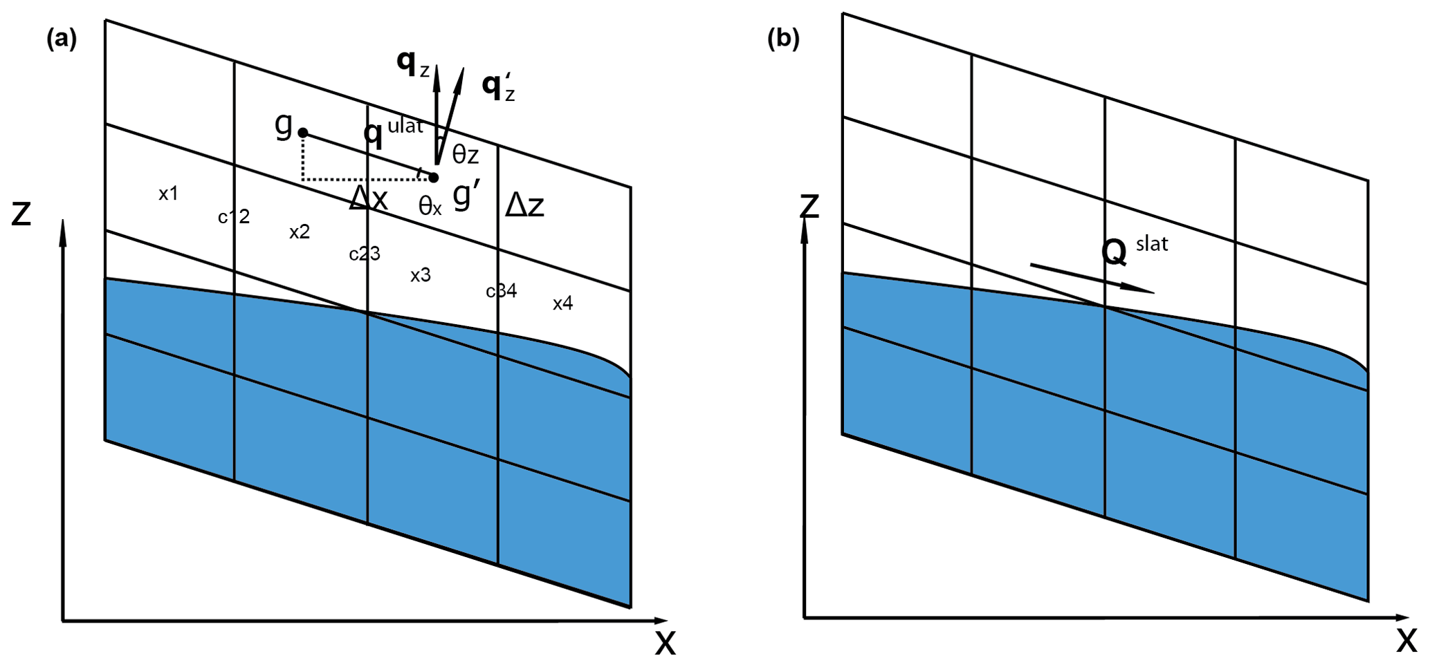
Figure 1Sketches of the terrain-following grid formulations, with illustrations of (a) unsaturated and (b) saturated subsurface lateral flow calculation. θx is the local angle of slope at the horizontal (x) direction, and θz is the angle between the normal vector of the cell surface and the vertical direction (z).
2.2 Lateral flow in saturated zone
The lateral flow in the saturated zone, Qslat (m−3 s−1), is also modeled using Darcy's law while taking the soil matric potential gradient as the groundwater hydraulic head gradient. In such a manner, the volumetric lateral groundwater flow can be given as
where w (m) is the width of the grid cell and T (m2 s−1) is the transmissivity. The transmissivity is calculated following the method used in Fan et al. (2007); see Appendix A. The Qslat is computed across inter-grid-cell scales using the same grid cell connections as used for the Qslat. The water table depth for each soil column within a grid cell is thereafter adjusted based on Qslat. Specifically, the Qslat increases and decreases the soil water content of the soil layer where the groundwater table is currently located. The soil moisture is updated while ensuring the soil moisture remains below and above the maximum and minimum allowable value. If the change in the soil moisture is less than the Qslat, the soil moisture of the layers above and below is recursively increased and decreased till the total change in soil moisture in all updated soil layers matches Qslat. In ELMv2.0, the groundwater table is adjusted by a conceptual recharge flux that depends on whether the water table is within or below the soil column. The approach by explicitly subtracting the hydrostatic equilibrium soil moisture distribution from the Richards equation resolved the numerical deficiencies when the water table is within the soil columns while using θ-based Richards equation (Zeng and Decker, 2009; Yu et al., 2014). In ELMlat, the water table is assumed within the soil columns, such that the conceptual recharge flux is no longer employed. The groundwater table depth is computed based on the soil water content following the θ-based water table method in CLM5.0 (Fig. 2). A no-flux boundary condition is applied to the last hydrologically active soil layer. Following ELMv2.0, the saturated zone is depleted by a drainage flux, i.e., the subsurface runoff, that is computed based on the SIMTOP scheme of Niu et al. (2007), with modifications to account for frozen soils (Oleson et al., 2013).
2.3 Model benchmarking against PFLOTRAN for idealized hillslopes
Three idealized hillslopes that included a convergent hillslope (CH), divergent hillslope (DH), and tilted V-shaped hillslope (VH) with variable saturated initial conditions are used to validate ELMlat by benchmarking against a 3D subsurface flow and transport model, PFLOTRAN.
2.3.1 Idealized hillslope geometries
The CH and DH problems have been widely used to test the newly developed lateral groundwater flow model, e.g., Troch et al. (2003); An et al. (2010); Hazenberg et al. (2015). Different from ELMv2.0, which uses uniform grid cells, the surface area of CH and DH grid cells change along the slope. The surfaces of CH and DH are curved by the sinusoidal function (Fig. 3):
where x, y, and z are the coordinates of the cell vertices. For the CH, the total width along the y direction linearly shrinks from 100 m at hill top to 80 m at hill bottom, whereas for the DH, it linearly expands from 80 m at hill top to 100 m at hill bottom (Fig. 3). The total width along the x direction is 100 m for both CH and DH.
The tilted V-catchment hillslope is another popular benchmark problem for validating groundwater flow in land surface models (Park et al., 2009; Sulis et al., 2011; Maxwell et al., 2014). As shown in Fig. 3c, the V-shaped catchment is formed by the union of two symmetrically inclined planar surfaces (80 m ×100 m) on the sides connected by a channel in the middle (20 m ×100 m). The two planar surfaces are inclined with slopes of ± 0.05 and 0.02 in the x and y directions, respectively. The channel is inclined following the slope of 0.02 in the y direction.
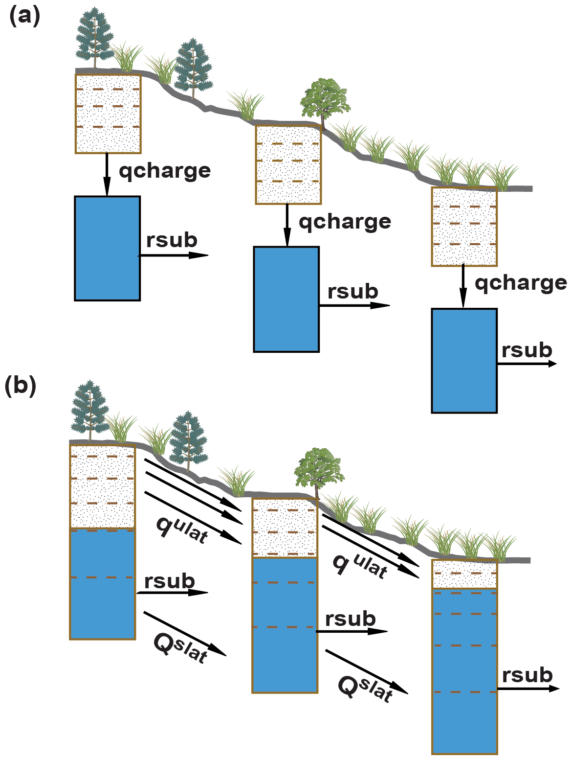
Figure 2Schematic illustration of the subsurface flow implementation in unsaturated and saturated zone from (a) ELMv2.0 to (b) ELMlat; qcharge is the conceptual recharge flux used to update the groundwater table, qulat is the lateral flux in unsaturated zone, qslat is the lateral flux in saturated zone, and rsub is the subsurface runoff.
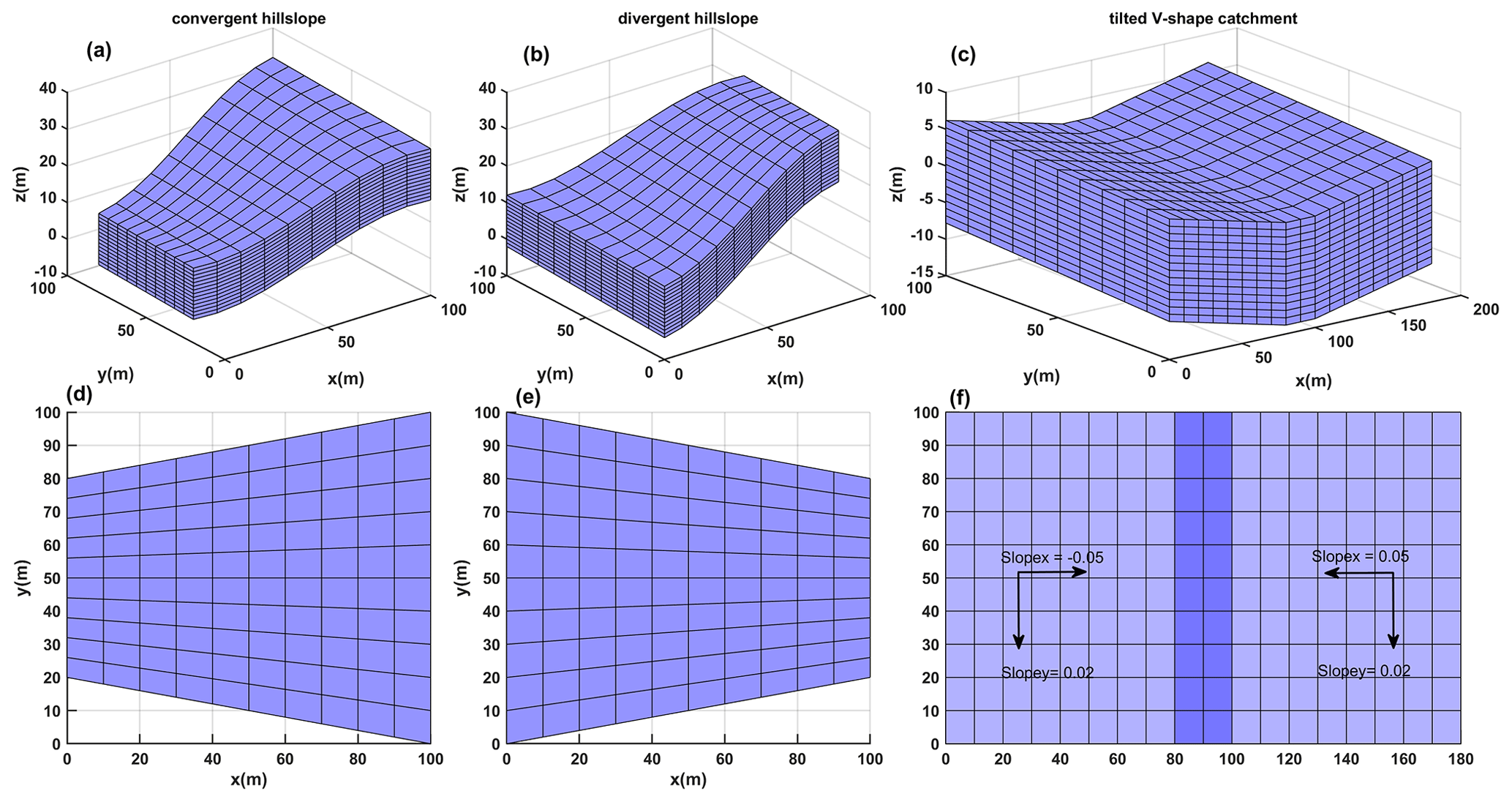
Figure 3Geometries of the three benchmark test problems. Panels (a), (b), and (c) are 3D views, and panels (d), (e), and (f) are x–y views of the three benchmark test problems, respectively. Sx and Sy are slopes along the x and y directions, respectively.
2.3.2 Model setup
By default, the soil columns of ELMv2.0 are vertically discretized into 15 soil layers of exponentially varying soil thicknesses reaching a depth of 42.1 m. Only the first 10 soil layers are hydrologically active and occupy the top 3.8 m of a soil column. For the model benchmarking, we modified the default model setup by allowing all 15 soil layers to be hydrological active and have a uniform soil thickness of 1 m to be consistent with the setup for PFLOTRAN simulations. The soil columns were horizontally discretized to a 10×10 mesh with a grid resolution of 10 m in the x direction and spatially changing resolution in the y direction for CH and DH. For VH, the soil columns were discretized horizontally with a uniform grid resolution of 10 m in both the x and y directions, which produced a mesh of 18×10. A homogeneous soil texture was used with a porosity of 0.467. The soil water retention properties in ELMv2.0 were described using the Clapp–Hornberger formula (Clapp and Hornberger, 1978), while in PFLOTRAN they were described using the Brooks–Corey formula (Brooks, 1965). We matched the soil water retention property parameters in PFLOTRAN with ELM. The translation of soil parameters between the two models is described in Appendix B. The anisotropic ratio for the horizontal to vertical hydraulic conductivity was set as 1.0 for the CH and DH cases () and 10.0 for the VH case (). We used a higher anisotropic ratio for the VH case to accelerate the lateral water movement for visualizing more evident soil moisture and groundwater dynamics. In order to evaluate the model sensitivity in response to the anisotropic ratio, we performed additional simulations using the anisotropic ratio of 10.0 for the CH and DH cases and 1.0 for the VH case. The same boundary and initial conditions were applied for the three benchmark problems. A no-flow boundary condition was applied on all sides of the domain. Hydrostatic pressure was used as the initial condition with the groundwater table depth (WTD) set at 7 m depth from the top surface. ELMlat and PFLOTRAN simulations were performed for 80 d for all three benchmark problems, and results were compared at the end of the simulation. The performance of soil moisture dynamics was evaluated using the mean absolute error (MAE) and root-mean-square error (RMSE) between ELMlat and PFLOTRAN, while the performance of groundwater was directly evaluated by the difference between ELMlat and PFLOTRAN simulations.
2.4 Model application
2.4.1 Study region
ELMlat is applied to study the role of lateral subsurface flow on terrestrial processes in the Little Washita Watershed (LWW), which is located in southwestern Oklahoma, USA (Fig. 4). The LWW has a drainage area of ≈611 km2 and is one of the seven selected experimental watersheds jointly administrated by the U.S. Department of Agriculture (USDA) and U.S. Environmental Protection Agency for a variety of hydrologic research projects. The LWW has a subhumid climate with annual precipitation of approximately 760 mm and annual temperature of approximately 16 ∘C. The elevation of LWW ranges from approximately 320 to 460 m, and the slope ranges from 0 to 3∘ (Fig. 4). Grassland is the dominant land cover of LWW, with small portions of land occupied with crops, shrubs, and deciduous trees. The mean annual leaf area index (LAI) is within the range of 0.5–3.0 m2 m−2. Soil textures of LWW are composed of sand, loam, and silty loam (Allen and Naney, 1991). LWW has a relatively high soil content of sand and organic matter in the northwestern part and southeastern part; several spots in the southern region have higher clay content (Fig. 4a–c).
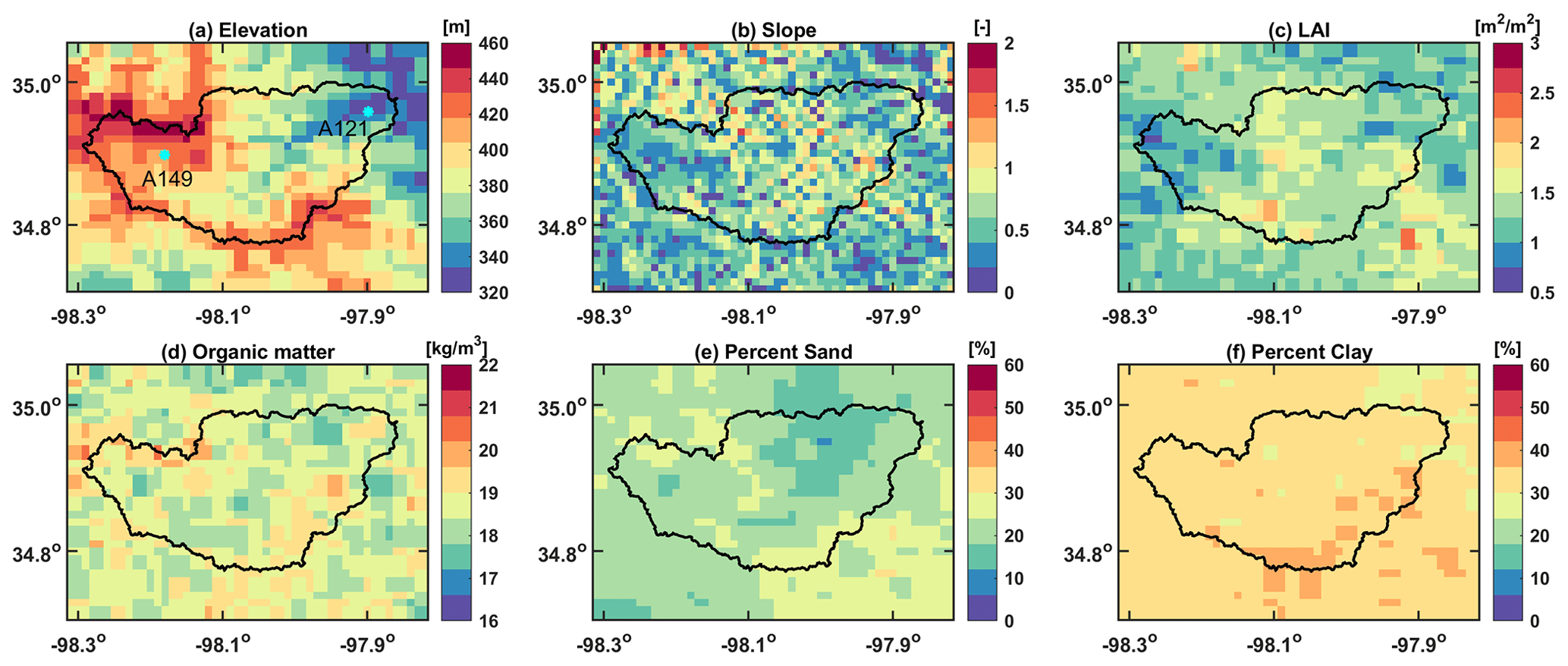
Figure 4Spatial distributions of (a) elevation, (b) slope, (c) mean monthly leaf area index, (d) organic matter density, and (e–f) percentages of sand and clay, respectively, over the study area at a resolution of 1 km.
2.4.2 Model configuration and data
The model domain covered a 35 km × 50 km area encompassing the LWW and was laterally discretized at 1 km × 1 km. All 15 soil layers were set as hydrologically active. Results from Fan et al. (2013) show the maximum WTD could reach up to 60 m deep in this region, which is deeper than the depth of ELM's 15-layer soil column. Therefore, we modified the soil thickness of the last two soil layers by adding 20 m each to their default values in ELMv2.0 while keeping the discretization of the other 13 soil layers unchanged. The total soil thickness could reach ≈82 m. The initial WTD was spatially uniformly set at 8 m deep below the top surface of the domain. The hourly NLDAS data (https://ldas.gsfc.nasa.gov/nldas/v2/forcing, last access: 5 December 2022) was used as the climate forcing which has a spatial resolution of 1/8∘ grid. We performed 100-year simulations with ELMlat and ELMv2.0 while cycling the atmospheric forcing data of 2008 to allow sufficient time for the model spin-up. The model results from the last year of the spin-up were used for analysis.
Friedl and Sulla-Menashe (2019)Myneni et al. (2021)Poggio et al. (2021)Poggio et al. (2021)Poggio et al. (2021)Jarvis et al. (2008)Table 1Specifications of high-resolution datasets used in this study.
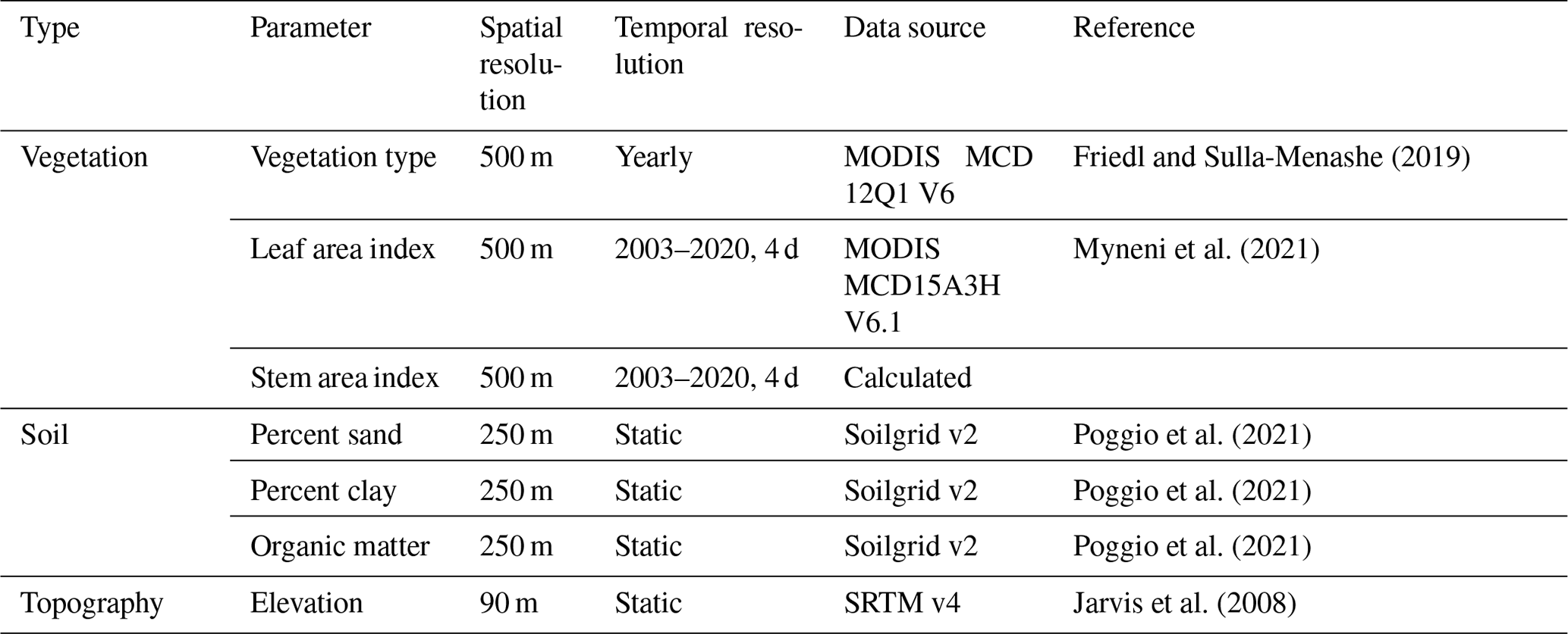
The recently developed 1 km surface data of Li et al. (2023) was used in this study, which was generated using multiple high-resolution, sub-kilometer datasets including vegetation-, soil-, and topography-related variables (Table 1). The soil, elevation, and LAI datasets were first aggregated to 1 km using the area-weighted average method, and the land cover data were aggregated to 1 km using the majority resampling method. Specifically, MODIS 500 m land cover was at year 2005 obtained from the Google Earth Engine (Gorelick et al., 2017, GEE). Following Ke et al. (2012), the LC_Type 5 class of MCD12Q1 v6 land cover product (Friedl and Sulla-Menashe, 2019) was used to determine the lake, urban, glacier, and vegetation plant functional types (PFTs). These PFTs were further classified into tropical, temperate, and boreal sub-types based on the rules presented in Bonan et al. (2002) and using meteorological data from WorldClim V1 (Hijmans et al., 2005). The monthly climatology LAI was derived from the 4 d MCD15A3H V6.1 (Myneni et al., 2021) over 2003–2020 using GEE. Then, based on the method in Zeng et al. (2002), we calculated the monthly climatology stem area index (SAI) from the LAI data. For the soil data, we used the Soilgrid v2 data with an original resolution of 250 m (Poggio et al., 2021). Soilgrid is generated based on machine learning using multiple data sources of soil profiles and remote sensing data (Hengl et al., 2017). The percent clay, percent sand, and soil organic matter at multiple depths were processed for ELM. The 90 m digital elevation from the Shuttle Radar Topography Mission (Jarvis et al., 2008) was used to derive topography-related parameters in ELM, including the standard deviation of elevation and slope. These 0.01∘ datasets were processed using GEE based on the original 90 m elevation.
The anisotropic ratio of the hydraulic conductivity has a close relationship with soil property because the platy mineral form and the low permeability of the clay content has a strong effect on the anisotropy (Fan et al., 2007). The anisotropic ratio is set as 10 () as used in Table 2 of Fan et al. (2007) based on the primary soil property of LWW. We used the WTD map (Fan et al., 2013), which is hereafter referred to as Fan2013, with a resolution of 30 arcsec (≈1 km) to validate the simulated WTD.
In ELMv2.0, the subsurface drainage flux (qd), which is calculated dependent on the water table depth (Niu et al., 2005), plays a role in regulating the long-term groundwater table:
where qd,max (kg m−2 s−1) is the maximum drainage flux that depends on the local slope of a grid cell and fd (m−1) is the subsurface drainage parameter. To improve the WTD simulations, the fd values were calibrated by performing an ensemble of simulations with fd values of 0.1, 0.5, 1.0, 2.5, 5.0, 10.0 m−1, respectively. A 100-year simulation was performed for each fd value, and the results from the last year of the simulation were employed for analysis. Following the approach of Bisht et al. (2018), a nonlinear functional relationship was established between the simulated WTD and fd values at each grid cell. The Fan2013 dataset was next employed to estimate an optimal fd based on the nonlinear WTD–fd relationship. The impacts of lateral flow on the model performance were assessed by comparing the soil moisture and energy fluxes including soil temperature and latent and sensible heat flux, with ELMv2.0 simulation. Site-level observations of soil moisture and soil temperature were collected from the ARS Micronetwork (https://ars.mesonet.org/, last access: 5 December 2022), which is operated and maintained by the USDA. The magnitude of unsaturated lateral flux against lateral flux was evaluated for both the idealized problems and the LWW. An experiment simulation on LWW was performed to evaluate the effects of unsaturated lateral flux on the energy fluxes by closing the unsaturated lateral flux while keeping the saturated lateral flux.
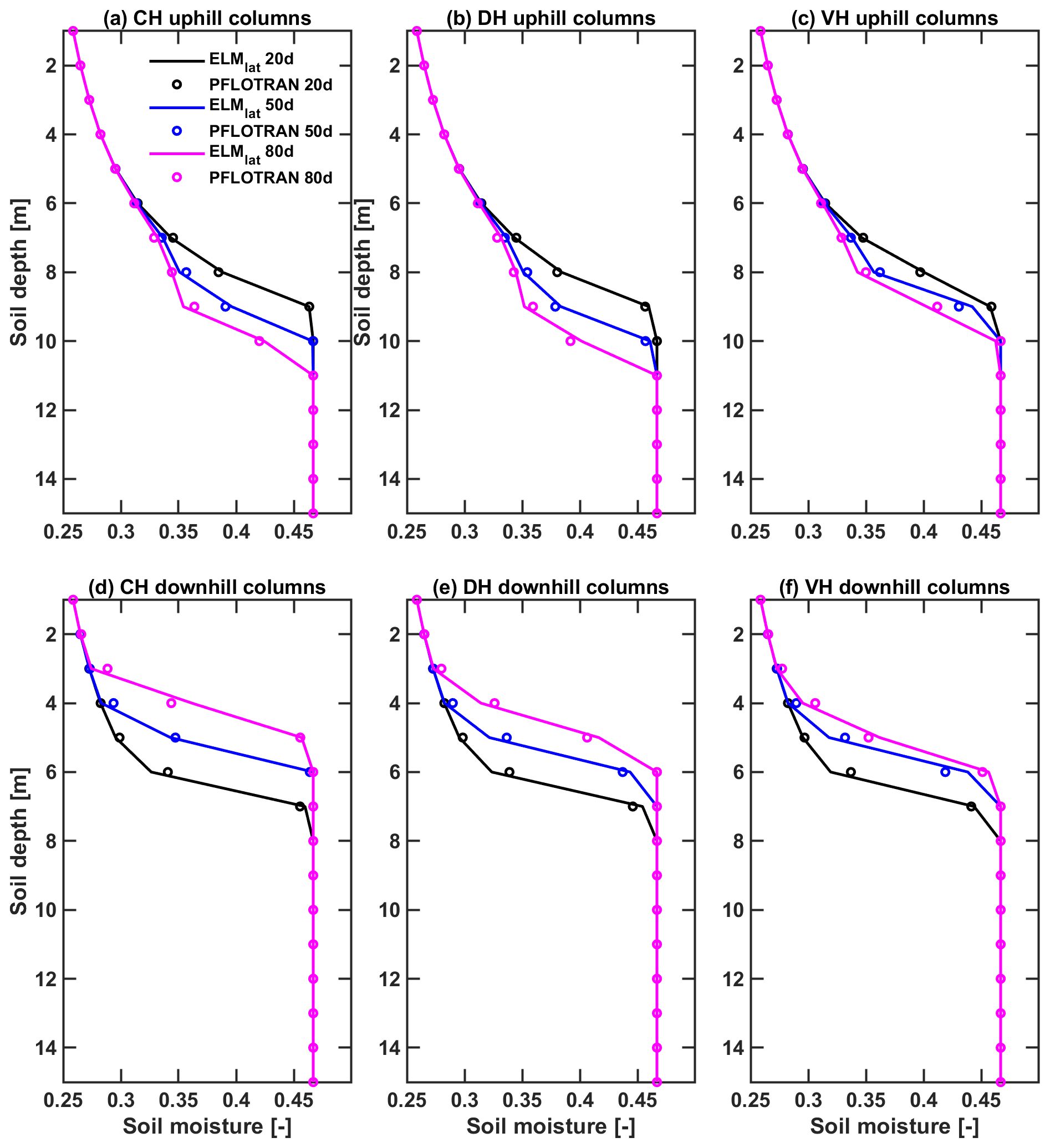
Figure 5The comparison of average soil moisture profile for the (a–c) uphill and (d–f) downhill columns by ELMlat (circles) and PFLOTRAN (lines) for the (a, d) convergent hillslope, (b, e) divergent hillslope, and (c, f) V-shaped hillslope. The results of the models are presented at the end of 20th, 50th, and 80th simulation day, respectively.
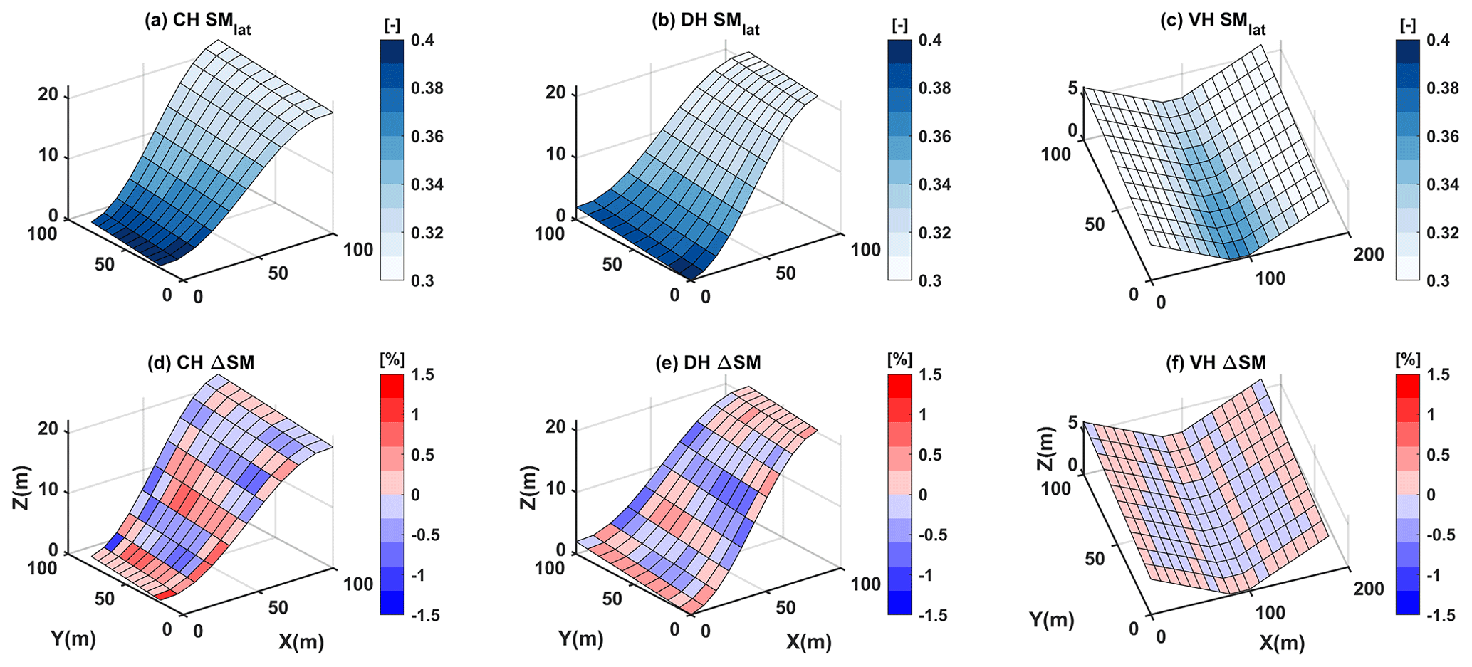
Figure 6ELMlat-simulated average soil moisture for the top 10 layers at the 80th simulation day for the (a) convergent hillslope, (b) divergent hillslope, and (c) V-shaped hillslope and the differences with PFLOTRAN for the (d) convergent hillslope, (e) divergent hillslope, and (f) V-shaped hillslope,.
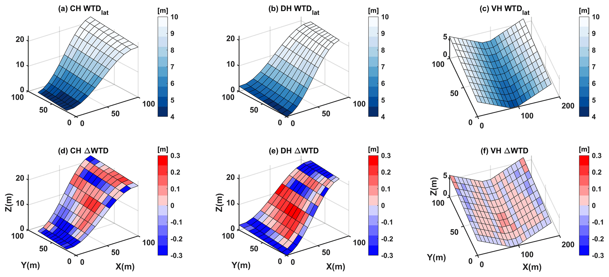
Figure 7ELMlat-simulated water table depth at the 80th simulation day for the (a) convergent hillslope, (b) divergent hillslope, and (c) V-shaped hillslope and the differences with PFLOTRAN for the (d) convergent hillslope, (e) divergent hillslope, and (f) V-shaped hillslope.
3.1 Evaluation of simulations for the benchmark problems
ELMlat can accurately reproduce the evolution of vertical soil moisture profile simulated by PFLOTRAN for all three benchmark problems (Fig. 5). The model correctly simulates the drying out of uphill soil columns (Fig. 5a–c) and the wetting up of downhill soil columns (Fig. 5d–f) for all the three hillslopes. In the VH case, the soil moisture shifted quickly during 20–50 d but slowed down during 50–80 d, whereas the rate of soil moisture change is nearly steady for the CH and DH cases during the two periods. During the period of 50–80 d, the VH case is much closer to a hydrostatic condition than the other two cases. The largest discrepancies in the simulated soil moisture are in soil layers that are closer to the water table, and these discrepancies could be explained by the differences in the model structure (Figs. A1 and A2). PFLOTRAN solves the variably saturated subsurface flow equation, which is applicable for both the unsaturated and saturated zones, while ELMlat has two separate flow models for the unsaturated and saturated zones. Thus, the difference between the two models is expected to be the largest near the unsaturated–saturated transition zone.
At the end of the simulation, the soil moisture was redistributed and transported following the surface topography via the lateral flow (Fig. 6a–c). The most downhill columns of CH and DH are approaching saturated, as shown in Fig. 6d–f. The difference between the two models was smaller than ±2 % for the top 10 layers on the 80th simulation day, which provides confidence in the ability of ELMlat to simulate lateral unsaturated soil moisture dynamics. During the simulation period, the MAEs in simulated ELMlat soil moisture for all cells in the top 10 soil layers remain within 1 %±3 % (Fig. A3a, c, e), and the RMSE for all three test problems remains within 0.04 (Fig. A3b, d, f).
At the end of the simulation, the simulated groundwater table evolves from the spatially uniform initial depth of 7 m below the top surface to a spatially varying depth that is inversely related to the surface elevation (Fig. 7a–c). In ELMlat, the lateral and vertical flow in unsaturated zone is carried out simultaneously in the same tridiagonal equation, while the saturated and unsaturated lateral flow is calculated sequentially. In PFLOTRAN, the saturated and unsaturated flow is simulated with a single variably saturated flow equation. Additionally, it should be noted that the prognostic variable in PFLOTRAN is the soil water pressure and the simulated WTD is diagnosed by linearly interpolating the vertical pressure profile for each soil column. Despite those differences, ELMlat-simulated WTD is comparable to that of PFLOTRAN with differences within ±0.2 m throughout the simulation period (Fig. A4).
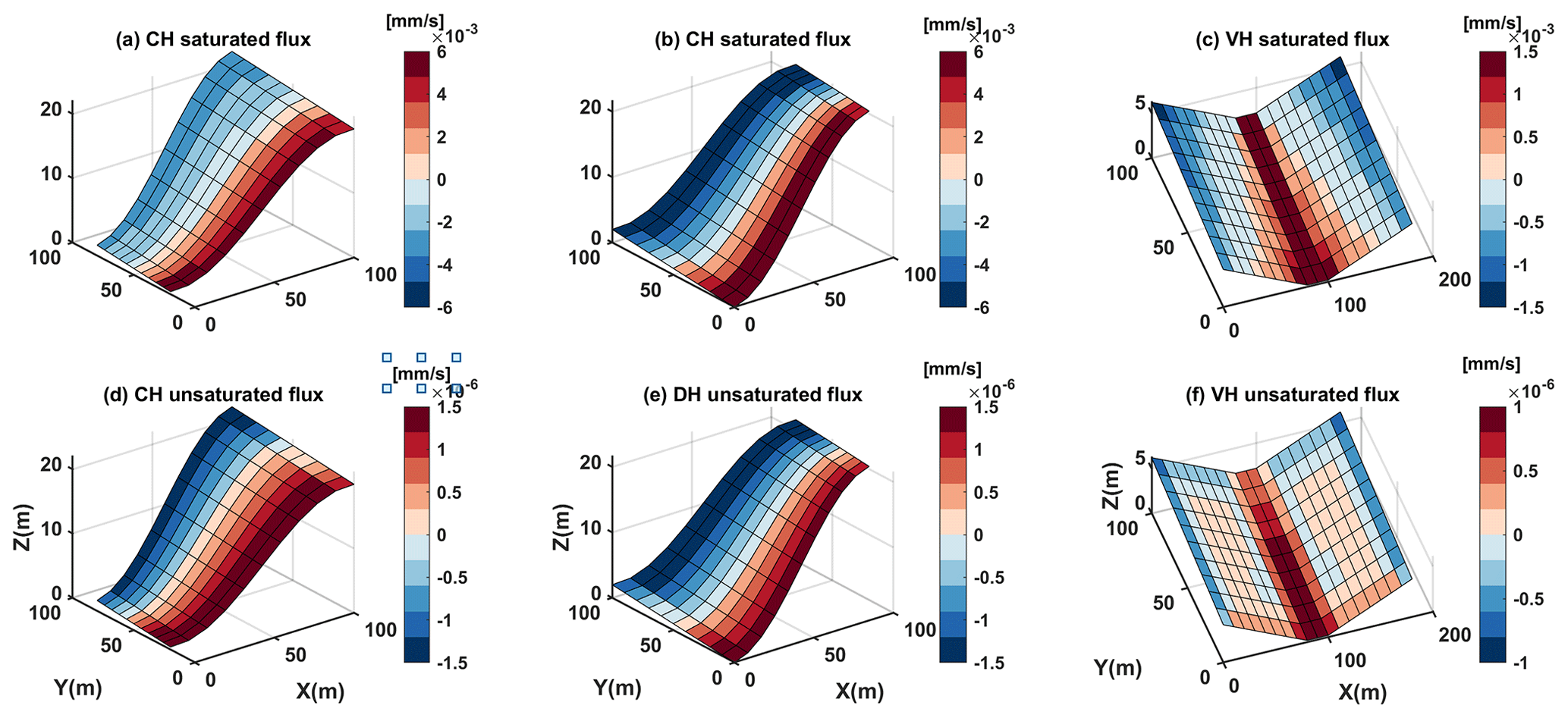
Figure 8The magnitude of saturated lateral flux vs. unsaturated lateral flux for the three idealized problems: panels (a), (b), (c) are the magnitude of saturated lateral fluxes for CH, DH, and VH problems, respectively, and panels (d), (e), (f) are the magnitude of unsaturated lateral flux for CH, DH, and VH problems, respectively.
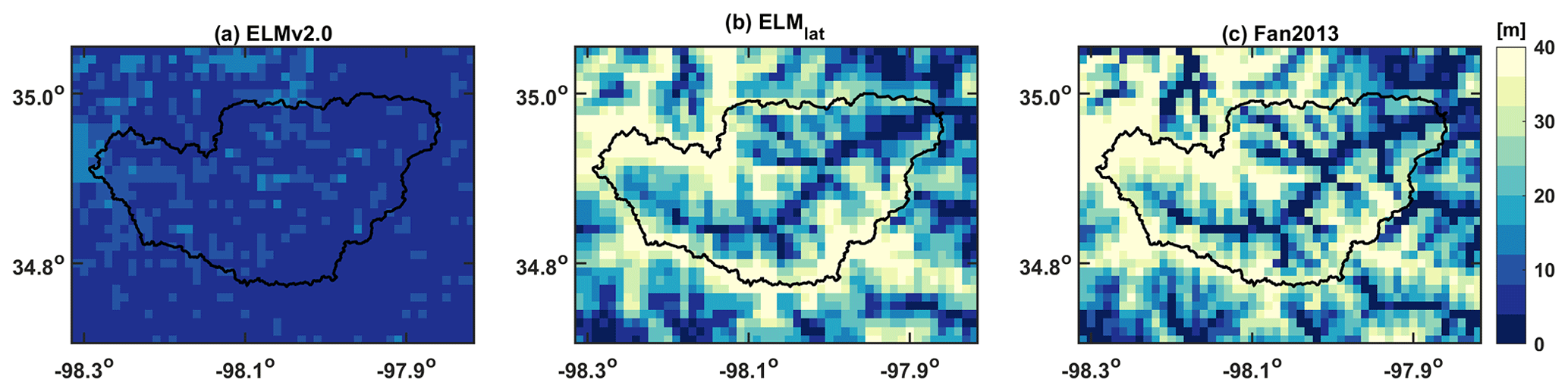
Figure 9Annual average groundwater table depth (WTD) simulated by (a) ELMv2.0, (b) ELMlat, and (c) the Fan2013 dataset.
For the CH and DH cases, which have a higher anisotropic ratio () and therefore larger lateral hydraulic conductivity and flow rate, the drying down on the up hills and wetting up on the down hills went much faster (Fig. A5a, b, d, e). The RMSE values of simulated soil moisture between ELMlat and PFLOTRAN for the top 10 soil layers for CH and DH are 0.016 and 0.017, respectively. These RMSE values are larger than the case with anisotropic ratio of 1.0, which were 0.011 and 0.0125 for CH and DH, respectively. For the VH cases with an anisotropic ratio of 1.0, water moves slowly since the average slope is low. The simulated results at the top 10 layers for the VH case are very close between the two models with RMSE value of 0.003, while the RMSE value for the higher anisotropic ratio is 0.010. Overall, the above evaluation results demonstrate that ELMlat can accurately represent vertical and lateral transport of soil moisture and groundwater.
Relative to lateral unsaturated groundwater flow, the lateral saturated groundwater flow is significantly larger. For all three benchmark cases, the magnitude of the unsaturated flow was mm s−1, while the magnitude of saturated flow is at mm s−1, as shown in Fig. 8. Hydraulic conductivity is nonlinearly dependent on soil saturation conditions and varies significantly with soil properties (Anderson et al., 2015). The scale difference in the hydraulic conductivity between unsaturated flow ( m s−1) and saturated flow ( m s−1) is the primary reason for the magnitude difference between unsaturated and saturated lateral flux.
3.2 Evaluation of simulations over LWW
Using the nonlinear relationship of WTD–fd, an optimized fd was obtained for 99 % of grid cells. Figure A6a shows an example of the WTD–fd relationship, and the spatial distribution of the calibrated fd value is shown in Fig. A6b. With optimized fd values, the simulated WTD dynamics in LWW simulated by ELMlat is significantly improved as compared to the ELMv2.0 results (Fig. 9). Simulated WTD by ELMlat showed a strong correlation (r2=0.85) with surface topography, which is consistent with the Fan2013 results (r2=0.87), while ELMv2.0-simulated WTD has no obvious spatial variations (Fig. 9).
Relative to ELMv2.0, including the lateral groundwater flow increased the baseflow of the runoff, as shown in Fig. A7. Redistributed WTD increased the subsurface runoff, while the timing of the peak runoff was not changed.
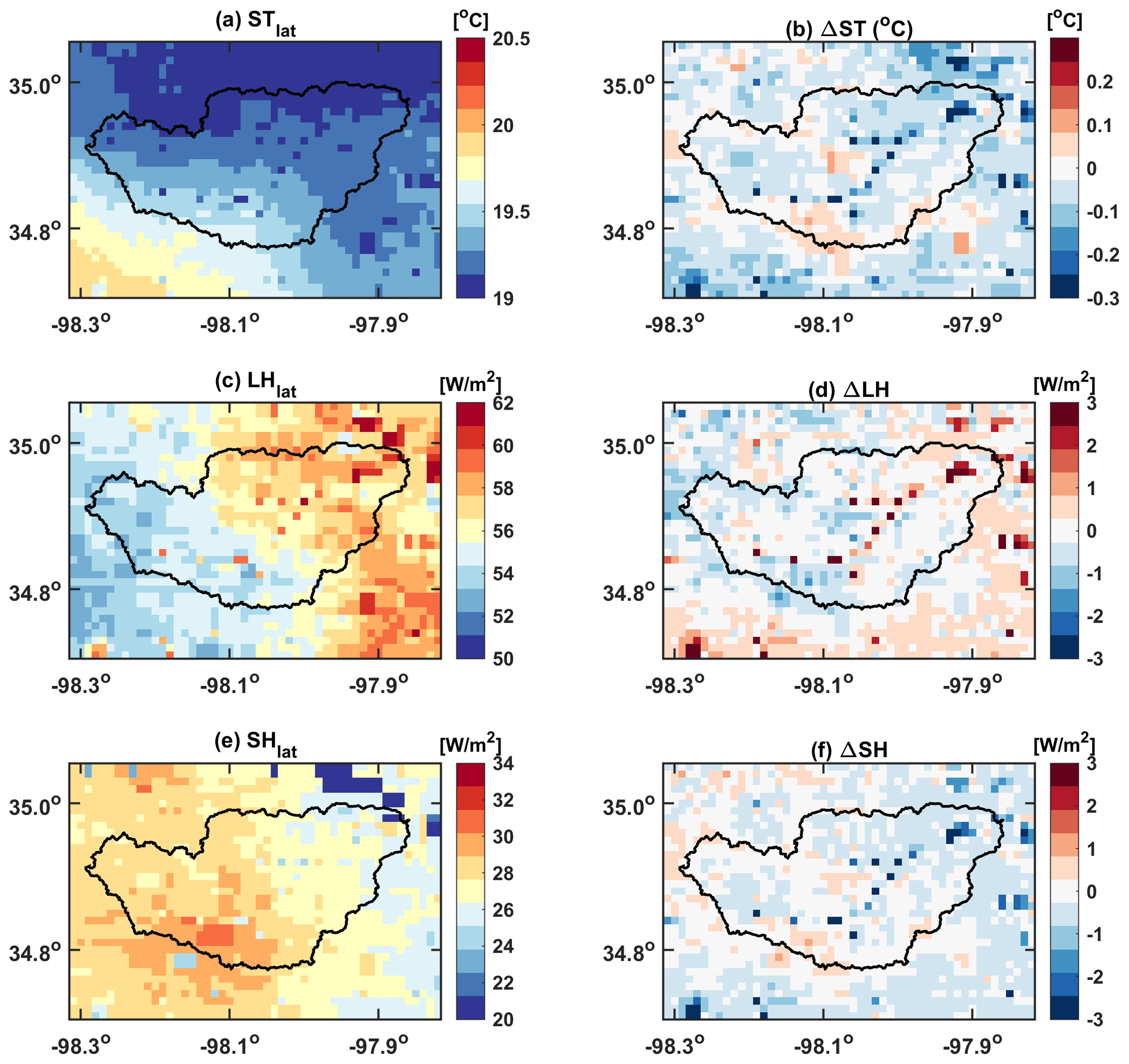
Figure 10ELMlat-simulated annual (a) top layer soil temperature (∘C), (c) latent heat flux (W m−2) and (e) sensible heat flux (W m−2). Panels (b), (d), and (f) are the differences between ELMlat and ELMv2.0 simulations for the three energy items, respectively.
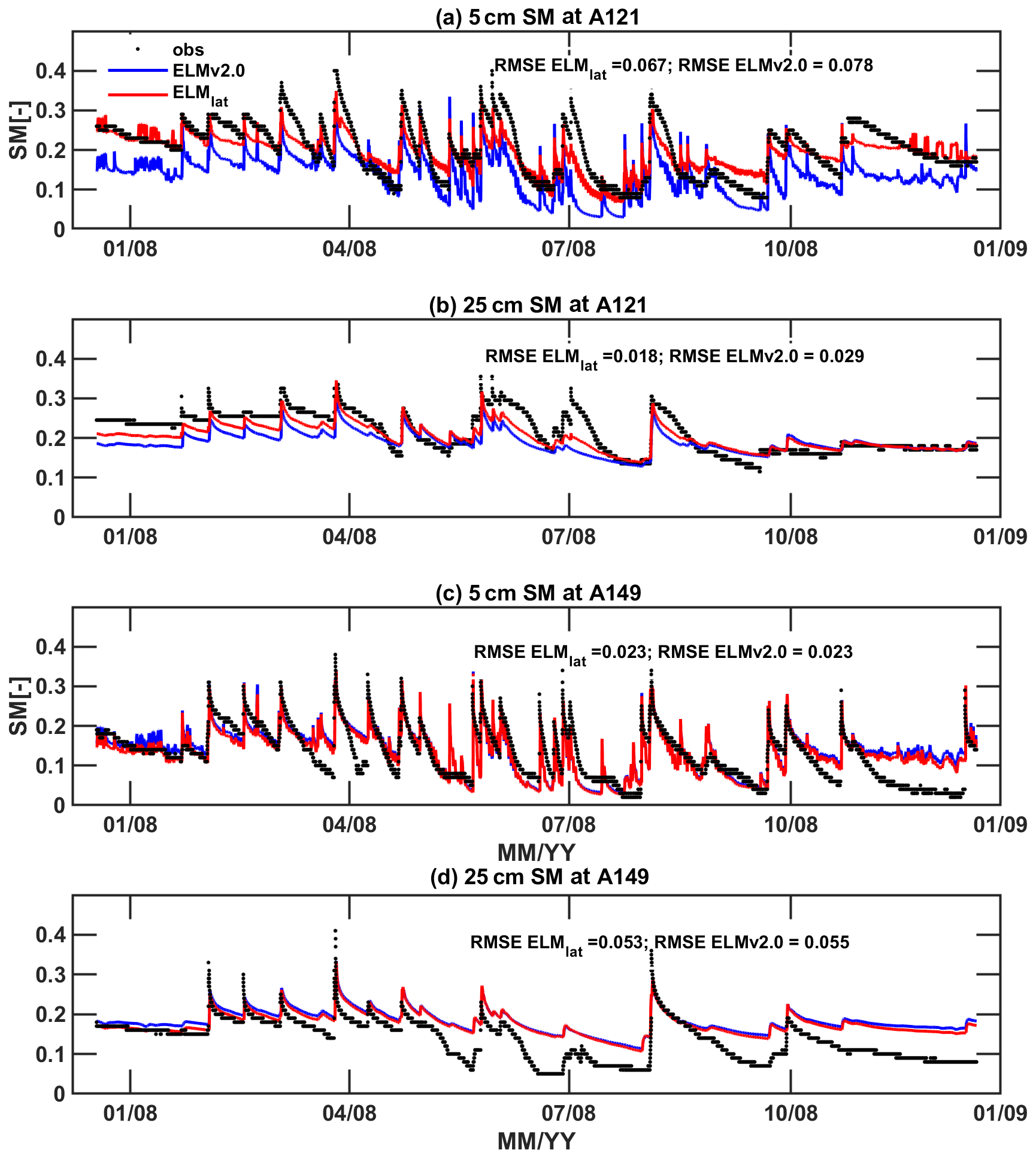
Figure 11Comparisons of simulated hourly soil moisture at depths of (a) 5 cm and (b) 25 cm of a lowland station (A121) and at depths of (c) 5 cm and (d) 25 cm of a high land station (A149) between ELMlat and ELMv2.0.
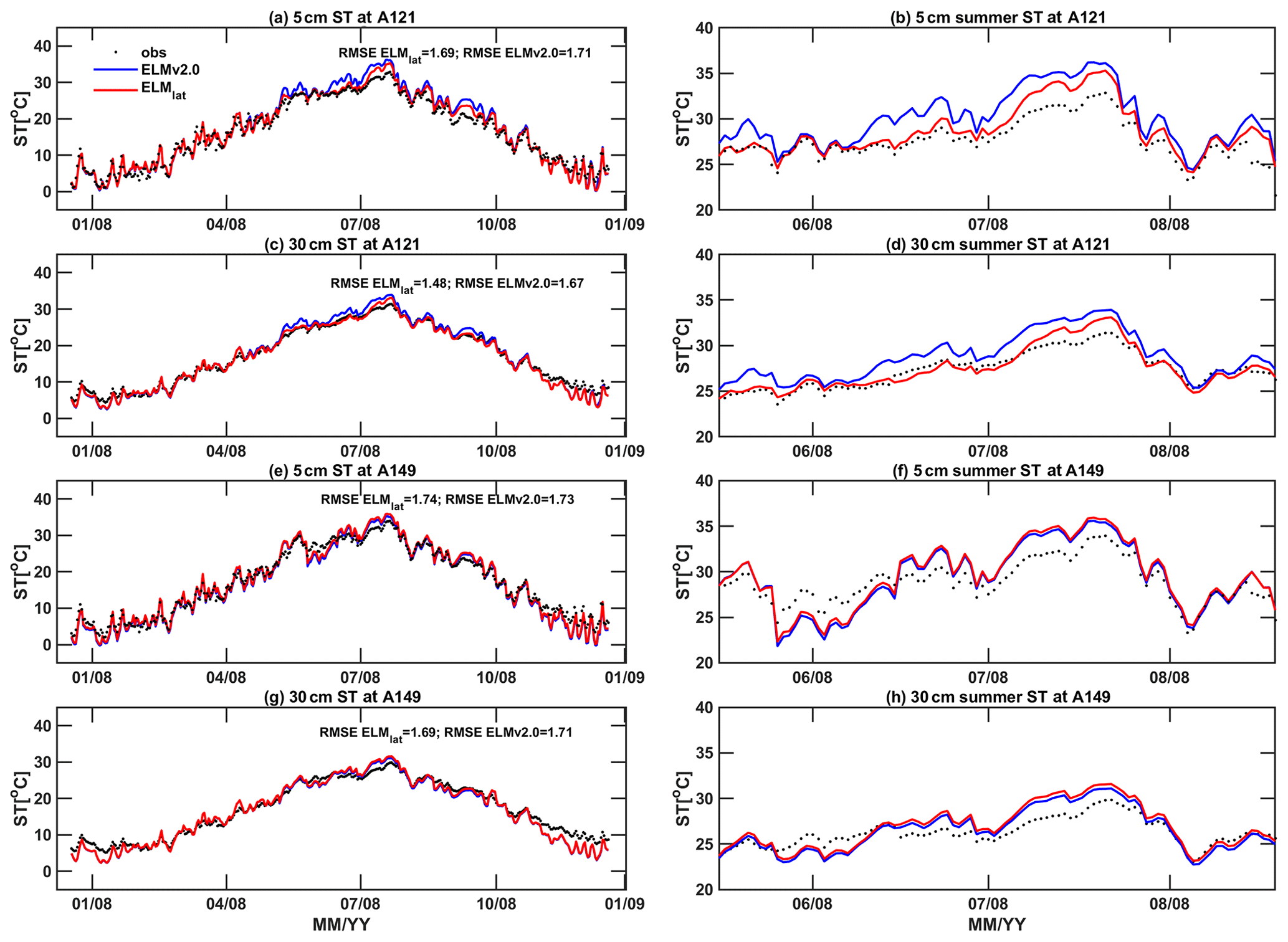
Figure 12Comparisons of simulated hourly annual and summer soil temperature at depths of 5 and 25 cm for a lowland station A121 and a highland station A149 between ELMlat and ELMv2.0: (a) 5 cm annual A121, (b) 5 cm summer A121, (c) 25 cm annual A121, (d) 25 cm summer A121, (e) 5 cm annual A149, (f) 5 cm summer A149, (g) 25 cm annual A149, and (h) 25 cm summer A149.
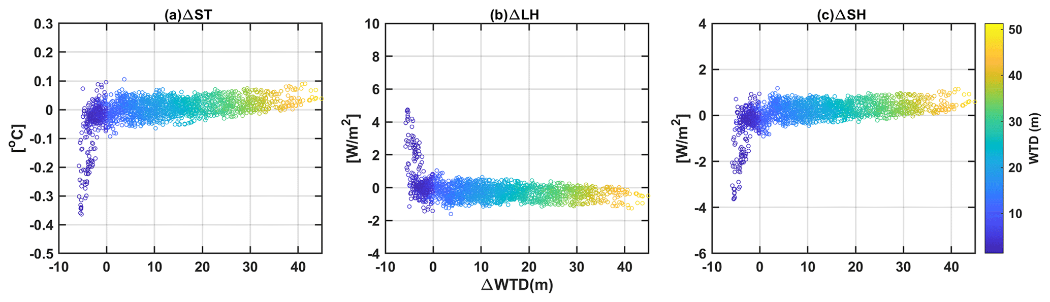
Figure 13Panels (a), (b), and (c) are the difference in annual average surface soil temperature, latent heat flux, and sensible heat flux between ELM-lat and ELMv2.0 vs. simulated groundwater depth differences between ELMlat and ELMv2.0. The color bar indicates the groundwater table depths simulated by ELMlat.
ELMlat simulated generally lower soil temperature (ST) and sensible heat flux (SH) but higher latent heat flux (LH) than ELMv2.0 for most of the grid cells (Fig. 10). The spatial annual ST showed a gradually increasing trend from north to south. The LH and SH showed the opposite spatial pattern, where LH is higher the SH is lower. The effects of WTD changes on the energy fluxes were more pronounced at low-elevation cells, especially at the stream and its surrounding cells. The delivery of the groundwater through the lateral flow to the valleys supported higher LH while reducing the SH compared with ELMv2.0 which has little spatial WTD variation.
Both ELMlat and ELMv2.0 were able to capture the major fluctuations and wetting–drying cycles of soil moisture (SM) by comparing observations at the two stations (Fig. 11). However, the dry-down rates of soil moisture results are not perfectly captured by both ELMlat and ELMv2.0. It should be noted that the simulated results represent the model behavior of the whole 1 km grid, while the measurements are taken at a single point. It is probable that the soil parameters for the 1 km grid could not accurately represent the soil property of the single point. Station A121 is located in the lowland area of this catchment with an elevation of 343 m while station A149 is located in the highland area with an elevation of 420 m (Fig. 4a). At station A121, ELMlat simulated higher soil moisture, with the annual mean 0.013 higher at 5 cm and 0.021 higher at 25 cm than ELMv2.0 results. At station A149, ELMlat simulated slightly lower soil moisture, with annual mean 0.007 lower at 5 cm and 0.009 lower than ELMv2.0 results.
For the soil temperature simulations, summer months show a larger change due to lateral subsurface flow; therefore, we focused our analysis on the summer temperature (Fig. 12). Relative to ELMv2.0, ELMlat simulated cooler summer temperature at both 5 (mean Δ ST ∘C) and 30 cm depths (mean Δ ST ∘C) at station A121. In contrast, at station A149, ELMlat simulated slightly higher summer temperatures at soil depths of 5 (mean Δ ST =0.017 ∘C) and 30 cm (mean Δ ST =0.019 ∘C). The differences in summer temperature between ELMlat and ELMv2.0 were consistent with the SH differences as discussed previously. The presence of higher soil moisture resulted in cooler summer soil temperature at station A121, whereas lower soil moisture resulted in increased summer soil temperature at station A149. However, both ELMlat and ELMv2.0 overestimated the temperature during July compared with observations, which may be due to the overestimation of incoming solar radiation or the discrepancies in the soil thermal properties between the model and reality at the sampled locations.
Lateral groundwater flow reshapes the groundwater table map and impacts the surface heat fluxes (Fig. 13). The most significant changes between ELMlat and ELMv2.0 in heat fluxes occur when ELMlat-simulated WTDs are less than 10 m, where ELMlat simulated generally shallower WTDs than ELMv2.0. As a result, ELMlat simulated lower surface soil temperature and lower SHs but higher LHs at shallower WTDs, which is consistent with previous discussions. The difference between surface soil temperature, LHs, and SHs are nearly linearly correlated with the WTD differences when the WTDs are less than 10 m. At deeper layers, the heat fluxes are not sensitive to changes in WTDs. The maximum differences in simulated surface soil temperature values could reach −0.3 to −0.4 ∘C, the LHs differences could reach 8–10 W m−2, and the SHs differences could reach −4 to −6 W m−2 at grids where ELMlat-simulated WTDs are less than 5 m. The depth at which groundwater can influence the vegetation functioning is dependent on the roots' penetration depths (Fan, 2015). However, since the land use type is quite simple in this watershed (e.g., mainly grass), it is difficult to differentiate the effects of WTD changes on the vegetation functions for different PFTs.
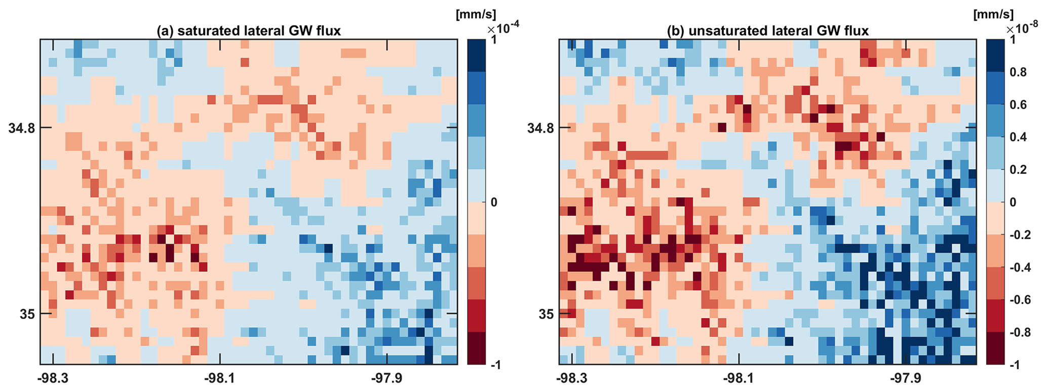
Figure 14The magnitude of (a) saturated lateral flux and (b) unsaturated lateral flux for Little Washita Watershed.
For the LWW case, the unsaturated groundwater flux is at a much lower magnitude relative to the saturated lateral flux (Fig. 14). The size of the unsaturated flow for LWW is at the magnitude of mm s−1, while the magnitude of saturated flow is at mm s−1. However, since unsaturated lateral flow is closer to the land surface relative to saturated flow, it still plays an important role in regulating the WTD and energy fluxes. Excluding unsaturated flow in ELMlat can result in the difference in simulated WTD in the range of ±0.04 m. The effect of unsaturated lateral flux on the energy fluxes is more pronounced right after a rainfall event (Fig. A8). Redistribution of soil moisture after the rainfall event significantly influenced the surface energy partitions. However, the redistributions are more confined in local areas, which indicates that it is not possible for the water to transport from upstream to downstream instantly after the rainfall through unsaturated flow. The energy flux change did not show a similar pattern for the land surface elevations of the whole watershed.
3.3 Caveats and future work
A homogeneous anisotropic ratio was assumed in the LWW study given the relatively uniform soil properties. Homogeneous aquifer depth or depth to bedrock (DTB) was also assumed in the LWW study. Brunke et al. (2016) evaluated the effects of using spatially heterogeneous soil thickness and sedimentary deposits (Pelletier et al., 2016) on the simulated hydrological and thermal fluxes in CLM4.5. Incorporating heterogeneous DTB in CLM4.5 has more impacts observed in locations with shallow bedrock than in deep bedrock on the water and energy fluxes reported by Brunke et al. (2016). Incorporation of variable DTB and evaluation of the heterogeneity of parameters will be performed in the future study.
This study is primarily oriented to validate the new features of the unsaturated and saturated lateral flow in ELM across grids and evaluate the connections between lateral groundwater flow and surface energy fluxes rather than rigidly close the water balance by calibrating all the water balance components against observations. Therefore, water balance and streamflow were not evaluated against observations in this study. A holistic evaluation of the impacts of the lateral groundwater flow on the water and energy balances, as well as the parameter sensitivities, will be tested and evaluated in a much larger domain in future work. In the present work, we have developed ELMlat that runs serially, and the model will be extended in the future to use high-performance computing to manage the high computational cost of global simulation. Research has found that the groundwater temperature can seasonally influence the surface water temperature and soil temperature (Hannah et al., 2004; Qiu et al., 2019). However, ELM assumes no heat flux boundary condition at the soil bottom, lacks lateral heat diffusion, and does not include advective heat transport. Uncertainties associated with the absence of these processes are to be explored in the future.
Additionally, some anthropogenic activities, e.g., groundwater pumping, irrigation, and two-way river–groundwater interactions are not incorporated into the current model structure. Extensive groundwater pumping reduced discharge to streams, with 10 %–23 % of watersheds reaching critical environmental flow thresholds, as revealed from large-scale groundwater modeling results (de Graaf et al., 2019). We envision a future road map with more holistic representations of hydrological functions building upon the lateral connections of the grid network, not exclusively the lateral groundwater flow, and more realized groundwater and surface water interactions in ELM.
Regarding the emerging highlights of lateral groundwater flow in the hyper-resolution large-scale Earth system modeling, we developed and validated an inter-grid-cell lateral groundwater flow model for both saturated and unsaturated zones in the E3SM Land Model framework.
By incorporating lateral groundwater flow in the ELMv2.0 and modifying the flux terms based on the non-horizontal terrain, the ELMlat could accurately simulate the soil moisture and WTD dynamics in three idealized hillslope problems validated against PFLOTRAN. During the simulation period, the MAE between the two models is within 1 %±3 %, and the RMSE is within 0.04. The simulated WTD differences are within ±0.2 m.
The developed model was further tested in a realistic watershed, i.e., Little Washita Watershed. The simulated WTD by ELMlat showed a strong correlation (r2=0.85) with surface topography, where higher land has a deeper groundwater table, which agreed well with the WTD pattern in Fan2013 of r2=0.87. The effects of lateral groundwater flow on the energy flux partitions were more pronounced at low-elevation areas with shallower groundwater tables (i.e., WTD <10 m). Lateral groundwater movement from highland area to the valleys cooled down the summer surface soil temperature at lowland areas; at highland areas, less water slightly increased the summer surface soil temperature. More water in the lowland area supported higher LH while reducing the SH compared with the ELMv2.0 simulation. In mountain areas with very deep WTDs (>10 m), the movement of lateral fluxes have relatively small effects on the surface energy fluxes relative to the effects at the lowland area. These results underscore the importance of including lateral groundwater flow in the LSMs, especially in the critical zone to holistically understand the role of groundwater system on the terrestrial water energy distribution and its feedback on climate change.
Following Fan et al. (2007), the transmissivity is calculated for two different cases: case 1 being the water table above 1.5 m depth, and case 2 being the water table below 1.5 m depth. The 1.5 m depth is chosen since the availability of reliable soil data is only to that depth.
For case 1 the following equations are used:
where m is soil layers number between the water table and the 1.5 m depth, Km (m s−1) denotes the hydraulic conductivity at layer m, and f (m) is the e-folding depth, the calculation of which will be explained later.
For case 2 the following equation is used:
where z (m) is the land surface elevation, h (m) is the water head, and (m) is the distance between the water table depth and the 1.5 m depth.
The calculation of the e-folding depth f is based on an empirical equation:
where a and b are constants and β is the terrain slope. In this study, a=120 m and b=150 m were used following the best fits estimated by Fan et al. (2007).
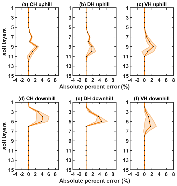
Figure A1Vertical absolute percent errors between ELMlat and PFLOTRAN at the most uphill column for (a) CH, (b) DH, and (c) VH and the most downhill column for (d) CH, (e) DH, and (f) VH for each layer at the 80th simulation day.
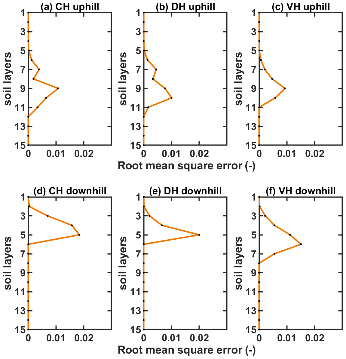
Figure A2Vertical root-mean-square errors between ELMlat and PFLOTRAN at the most uphill column for (a) CH, (b) DH, and (c) VH and the most downhill column for (d) CH, (e) DH, and (f) VH for each layer at the 80th simulation day.
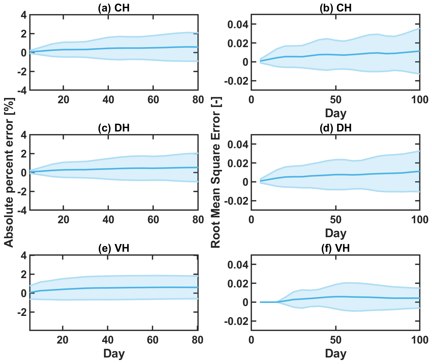
Figure A3The mean absolute error (a, c, e) and root-mean-square error (b, d, f) of simulated soil moisture between ELMlat and PFLOTRAN for the top 10 soil layers during the simulation period.
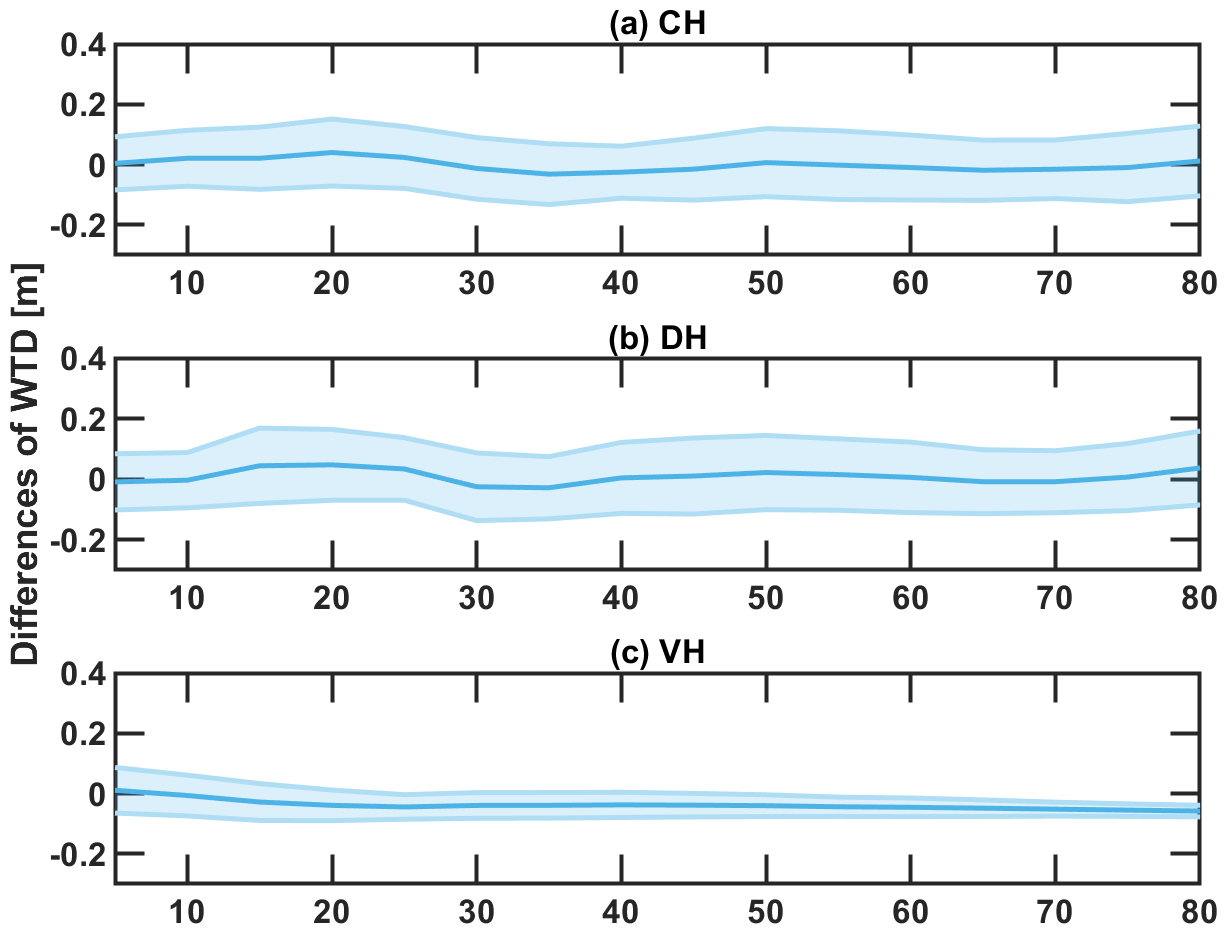
Figure A4The differences in simulated groundwater table depths between ELMlat and PFLOTRAN during the simulation period.
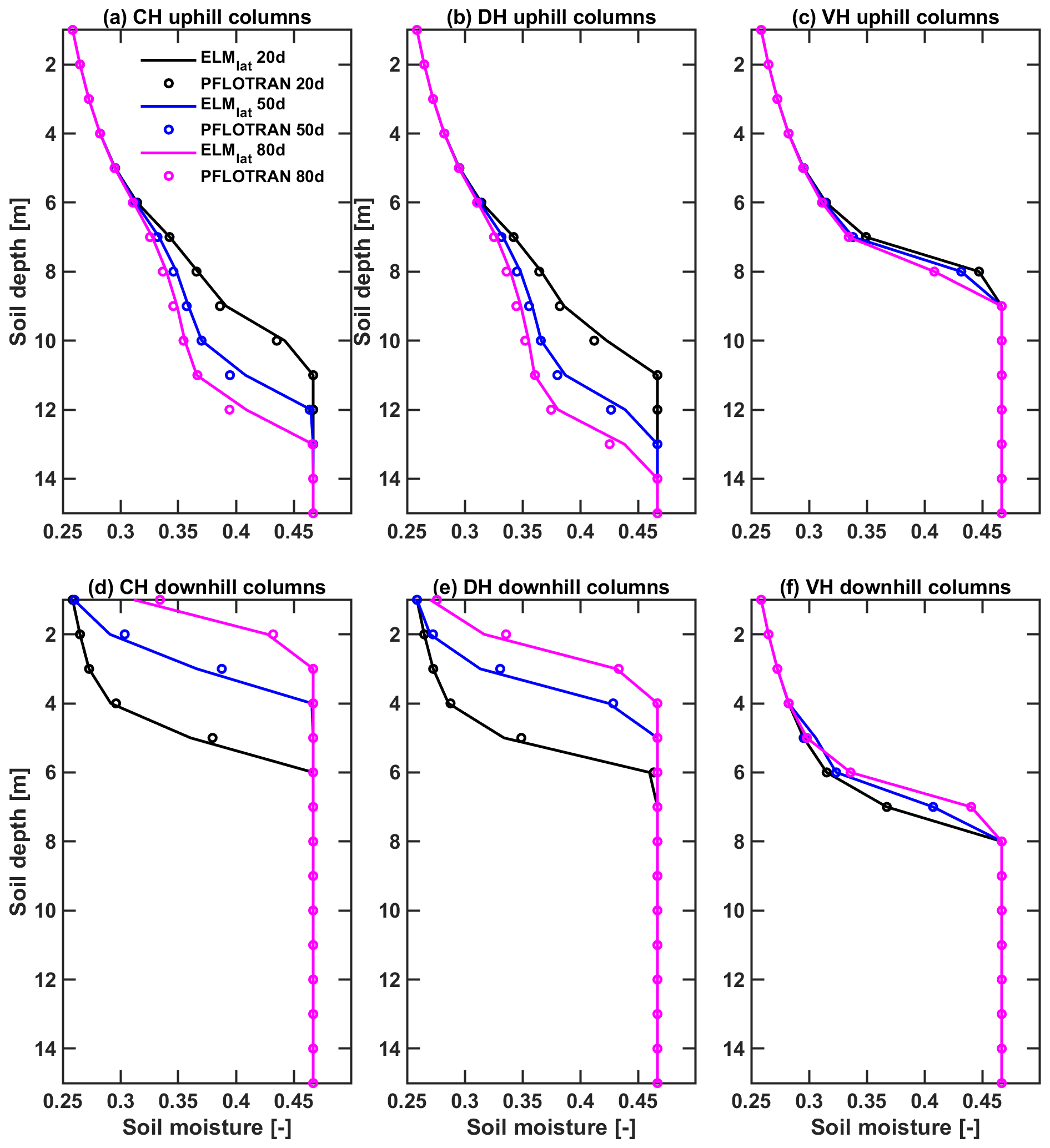
Figure A5ELMlat vs. PFLOTRAN simulated mean soil moisture profile for the 10 uphill columns of the (a) convergent hillslope (b) divergent hillslope, and (c) V-shaped hillslope and 10 downhill columns of the (d) convergent hillslope, (e) divergent hillslope, and (f) V-shaped hillslope at the 20th, 50th and 80th simulation day, respectively. For the convergent hillslope and the divergent hillslope, the anisotropic ratio is 10. For the V-shaped hillslope, the anisotropic ratio is 1.
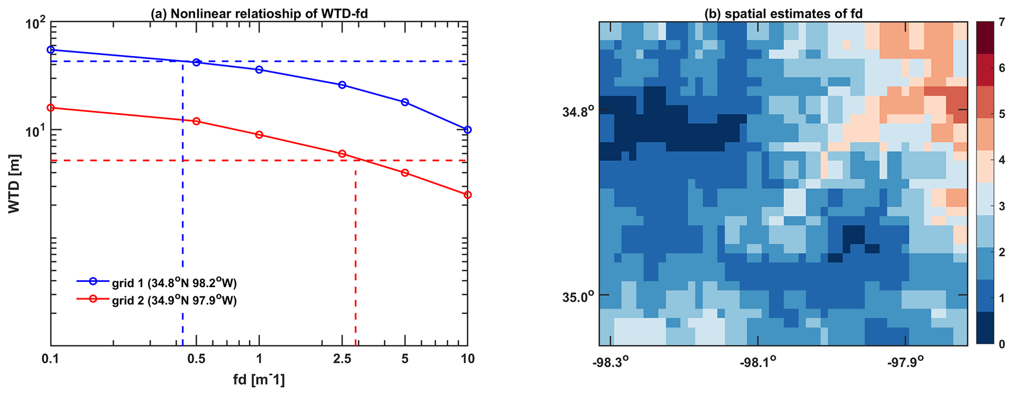
Figure A6(a) An example of establishing the nonlinear functional relationship of WTD-fd and (b) the spatial distribution of calibrated fd values.
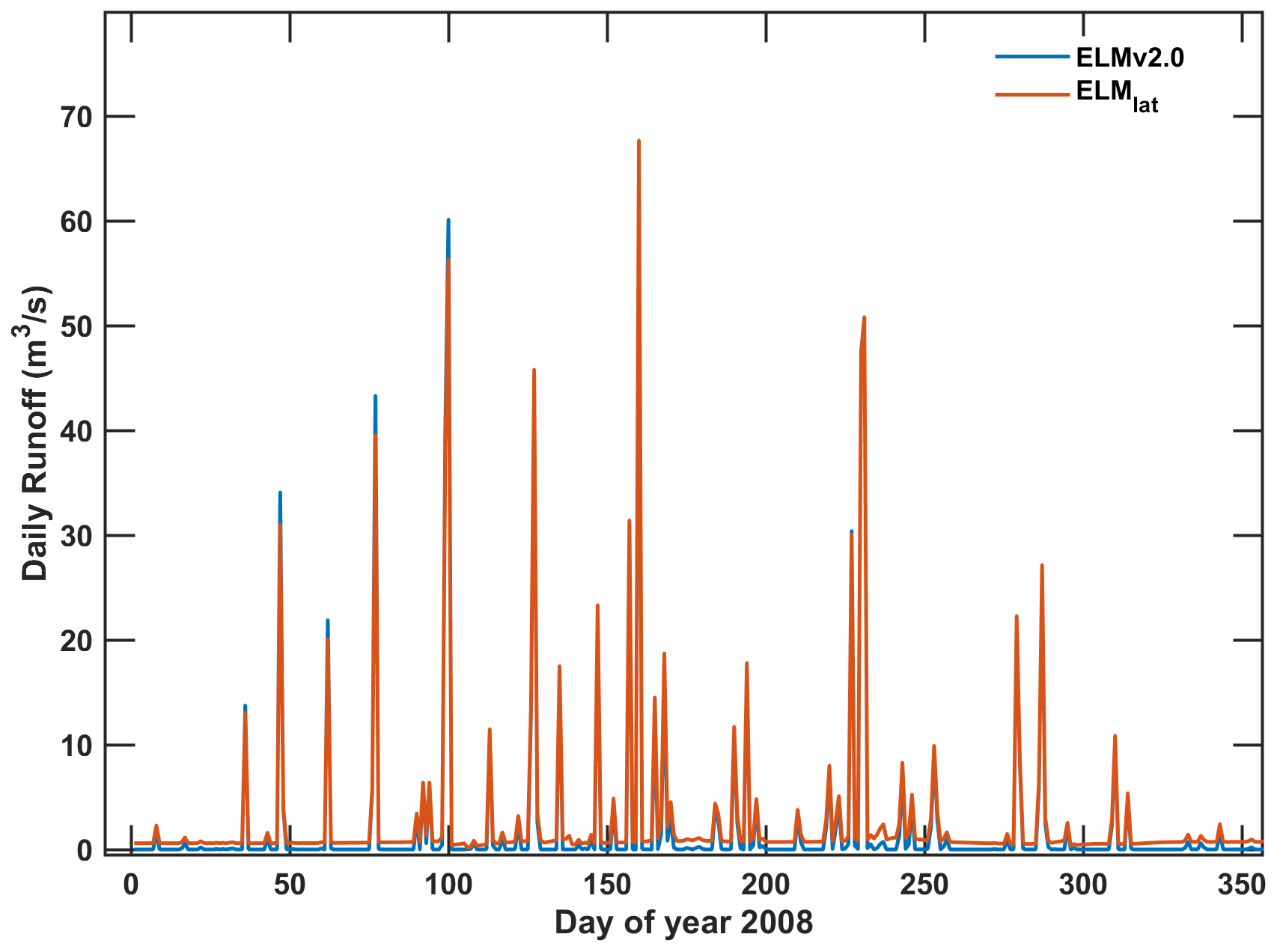
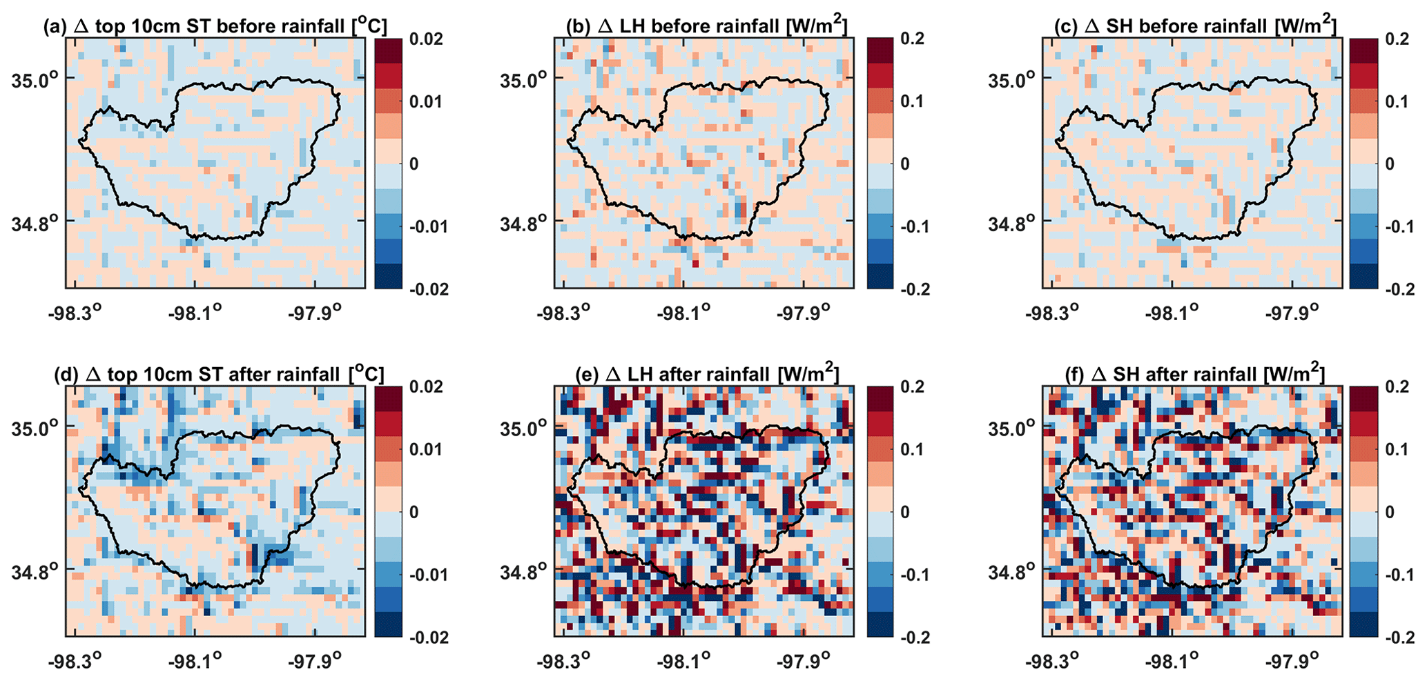
Figure A8The energy flux changes for the top 10 cm soil of Little Washita Watershed after excluding unsaturated later flux for the day before and after a rainfall event during 6–7 July: panels (a), (b), and (c) are the soil temperature, latent heat flux, and sensible heat flux changes the day before the rainfall event, respectively, while (d), (e), and (f) are the soil temperature, latent heat flux, and sensible heat flux changes the day after the rainfall event, respectively.
ELM uses the Clapp–Hornberger formula (Clapp and Hornberger, 1978) for parameterizing the soil water retention properties, as shown in Eq. (10), while PFLOTRAN uses the Brooks–Corey (Brooks, 1965) formula to parameterize the soil water retention properties. For the Burdine–Brooks–Corey water retention formula, the effective saturation, se (no unit), can be expressed as
where sw (no unit) is the soil saturation and sr (no unit) is the residual saturation; Pc (Pa) is the capillary pressure, Pa is the air entry pressure, and λ (no unit) is a parameter. In unsaturated conditions and assuming sr=0:
PFLOTRAN uses the relative permeability, kr, instead of hydraulic conductivity involved in the calculation of the Richards equation, where the relative permeability can be calculated as follows:
where λ is a parameter.
The transformation of the parameter between the two models can be expressed as follows:
By performing this transformation and assuming sr=0, the two water retention curves are very similar except for the difference when using terms of hydraulic conductivity against effective permeability.
Data files and running scripts for model simulations are available at https://doi.org/10.5281/zenodo.7659300 (Qiu et al., 2023a). The ELMlat model is available at https://doi.org/10.5281/zenodo.7686303 (Qiu et al., 2023b) for the idealized hillslope problems and at https://doi.org/10.5281/zenodo.7686381 (Qiu et al., 2023c) for the LWW application. E3SMv2.0 (including ELMv2.0) is supported by the Linux system.
The details for running E3SMv2.0 (including ELMv2.0) can be found at https://e3sm.org/model/running-e3sm/e3sm-quick-start/ (E3SM developer team, 2022). ELMlat adopts the same compilation and running approaches. PFLOTRAN can be installed and compiled on Linux, Mac, and Windows systems. The detailed instructions for PFLOTRAN installation and running are provided by the user's guide at https://www.pflotran.org/documentation/user_guide/user_guide.html (PFLOTRAN developer team, 2022).
HQ designed the study, developed the model, processed the data, and prepared the original manuscript. GB designed the study, discussed the results, and edited the paper LL, DH, and DX processed the data, contributed to subsequent analysis, and helped write and edit the manuscript.
The contact author has declared that none of the authors has any competing interests.
Publisher's note: Copernicus Publications remains neutral with regard to jurisdictional claims made in the text, published maps, institutional affiliations, or any other geographical representation in this paper. While Copernicus Publications makes every effort to include appropriate place names, the final responsibility lies with the authors.
The work reported in this paper was conducted at Pacific Northwest National Laboratory, which is operated for the U.S. Department of Energy by Battelle Memorial Institute under contract DE-AC05-76RL01830. The simulations for this research were performed on the CompyMcNodeFace, a computer system of the U.S. Department of Energy, Office of Biological and Environmental Research.
This research has been supported by the U.S. Department of Energy (grant no. DE-AC05-76RL01830).
This paper was edited by Taesam Lee and reviewed by Zhenghui Xie and two anonymous referees.
Allen, P. B. and Naney, J. W.: Hydrology of the Little Washita River Watershed, Oklahoma: data and analyses, Technical report, Agricultural Research Service, U.S. Dept. of Agriculture, Durant, Ohio, https://www.ars.usda.gov/plains-area/el-reno-ok/ocparc/agroclimate-and-hydraulics-research-unit/docs/docs-from-anrr/docs/hydrology-of-the-little-washita-river-watershed/ (last access: 20 December 2023), 1991. a
An, H., Ichikawa, Y., Tachikawa, Y., and Shiiba, M.: Three-dimensional finite difference saturated-unsaturated flow modeling with nonorthogonal grids using a coordinate transformation method, Water Resour. Res., 46, https://doi.org/10.1029/2009WR009024, 2010. a
Anderson, M. P., Woessner, W. W., and Hunt, R. J.: Applied groundwater modeling: simulation of flow and advective transport, Academic press, https://doi.org/10.1016/C2009-0-21563-7, 2015. a
Archfield, S.A., Clark, M., Arheimer, B., Hay, L.E., McMillan, H., Kiang, J.E., Seibert, J., Hakala, K., Bock, A., Wagener, T., Farmer, W.H., Andréassian, V., Attinger, S., Viglione, A., Knight, R., Markstrom, S., and Over, T.: Accelerating advances in continental domain hydrologic modeling, Water Resour. Res., 51, 10078–10091, 2015. a, b
Bierkens, M. F. P., Bell, V. A., Burek, P., Chaney, N., Condon, L. E., David, C. H., de Roo, A., Döll, P., Drost, N., Famiglietti, J. S., Flörke, M., Gochis, D. J., Houser, P., Hut, R., Keune, J., Kollet, S., Maxwell, R. M., Reager, J. T., Samaniego, L., Sudicky, E., Sutanudjaja, E. H., van de Giesen, N., Winsemius, H., and Wood, E. F.: Hyper-resolution global hydrological modelling: what is next? “Everywhere and locally relevant”, Hydrol. Process., 29, 310–320, 2015. a
Bisht, G., Huang, M., Zhou, T., Chen, X., Dai, H., Hammond, G. E., Riley, W. J., Downs, J. L., Liu, Y., and Zachara, J. M.: Coupling a three-dimensional subsurface flow and transport model with a land surface model to simulate stream–aquifer–land interactions (CP v1.0), Geosci. Model Dev., 10, 4539–4562, https://doi.org/10.5194/gmd-10-4539-2017, 2017. a
Bisht, G., Riley, W. J., Hammond, G. E., and Lorenzetti, D. M.: Development and evaluation of a variably saturated flow model in the global E3SM Land Model (ELM) version 1.0, Geosci. Model Dev., 11, 4085–4102, https://doi.org/10.5194/gmd-11-4085-2018, 2018. a
Bonan, G. B., Levis, S., Kergoat, L., and Oleson, K. W.: Landscapes as patches of plant functional types: An integrating concept for climate and ecosystem models, Global Biogeochem. Cy., 16, 5-1–5-23, https://doi.org/10.1029/2000GB001360, 2002. a
Brooks, R. H.: Hydraulic properties of porous media, Colorado State University, 1965. a, b
Brunke, M. A., Broxton, P., Pelletier, J., Gochis, D., Hazenberg, P., Lawrence, D. M., Leung, L. R., Niu, G.-Y., Troch, P. A., and Zeng, X.: Implementing and evaluating variable soil thickness in the Community Land Model, version 4.5 (CLM4.5), J. Climate, 29, 3441–3461, 2016. a, b
Celia, M. A., Bouloutas, E. T., and Zarba, R. L.: A general mass-conservative numerical solution for the unsaturated flow equation, Water Resour. Res., 26, 1483–1496, 1990. a
Chaney, N. W., Metcalfe, P., and Wood, E. F.: HydroBlocks: a field-scale resolving land surface model for application over continental extents, Hydrol. Process., 30, 3543–3559, 2016. a
Chaney, N. W., Torres-Rojas, L., Vergopolan, N., and Fisher, C. K.: HydroBlocks v0.2: enabling a field-scale two-way coupling between the land surface and river networks in Earth system models, Geosci. Model Dev., 14, 6813–6832, https://doi.org/10.5194/gmd-14-6813-2021, 2021. a
Childs, E.: Drainage of groundwater resting on a sloping bed, Water Resour. Res., 7, 1256–1263, 1971. a, b
Chui, T. F. M., Low, S. Y., and Liong, S.-Y.: An ecohydrological model for studying groundwater–vegetation interactions in wetlands, J. Hydrol., 409, 291–304, 2011. a
Clapp, R. B. and Hornberger, G. M.: Empirical equations for some soil hydraulic properties, Water Resour. Res., 14, 601–604, https://doi.org/10.1029/WR014i004p00601, 1978. a, b, c
Clark, M. P., Fan, Y., Lawrence, D. M., Adam, J. C., Bolster, D., Gochis, D. J., Hooper, R. P., Kumar, M., Leung, L. R., Mackay, D. S., Maxwell, R. M., Shen, C., Swenson, S. C., and Zeng, X.: Improving the representation of hydrologic processes in Earth System Models, Water Resour. Res., 51, 5929–5956, https://doi.org/10.1002/2015WR017096, 2015. a, b
Condon, L. E. and Maxwell, R. M.: Simulating the sensitivity of evapotranspiration and streamflow to large-scale groundwater depletion, Sci. Adv., 5, eaav4574, https://doi.org/10.1126/sciadv.aav4574, 2019. a, b
De Graaf, I., Van Beek, L., Wada, Y., and Bierkens, M.: Dynamic attribution of global water demand to surface water and groundwater resources: Effects of abstractions and return flows on river discharges, Adv. Water Resour., 64, 21–33, 2014. a
de Graaf, I. E., van Beek, R. L., Gleeson, T., Moosdorf, N., Schmitz, O., Sutanudjaja, E. H., and Bierkens, M. F.: A global-scale two-layer transient groundwater model: Development and application to groundwater depletion, Adv. Water Resour., 102, 53–67, 2017. a
de Graaf, I. E., Gleeson, T., Van Beek, L., Sutanudjaja, E. H., and Bierkens, M. F.: Environmental flow limits to global groundwater pumping, Nature, 574, 90–94, 2019. a
Döll, P., Hoffmann-Dobrev, H., Portmann, F. T., Siebert, S., Eicker, A., Rodell, M., Strassberg, G., and Scanlon, B.: Impact of water withdrawals from groundwater and surface water on continental water storage variations, J. Geodyn., 59, 143–156, 2012. a
E3SM developer team: E3SM quick start, https://e3sm.org/model/running-e3sm/e3sm-quick-start/, 2022. a
Eyring, V., Bony, S., Meehl, G. A., Senior, C. A., Stevens, B., Stouffer, R. J., and Taylor, K. E.: Overview of the Coupled Model Intercomparison Project Phase 6 (CMIP6) experimental design and organization, Geosci. Model Dev., 9, 1937–1958, https://doi.org/10.5194/gmd-9-1937-2016, 2016. a
Fan, Y.: Groundwater in the E arth's critical zone: Relevance to large-scale patterns and processes, Water Resour. Res., 51, 3052–3069, 2015. a, b, c
Fan, Y., Miguez-Macho, G., Weaver, C. P., Walko, R., and Robock, A.: Incorporating water table dynamics in climate modeling: 1. Water table observations and equilibrium water table simulations, J. Geophys. Res.-Atmos., 112, https://doi.org/10.1029/2006JD008111, 2007. a, b, c, d, e, f
Fan, Y., Li, H., and Miguez-Macho, G.: Global patterns of groundwater table depth, Science, 339, 940–943, 2013. a, b
Fan, Y., Clark, M., Lawrence, D. M., Swenson, S., Band, L. E., Brantley, S. L., Brooks, P. D., Dietrich, W. E., Flores, A., Grant, G., Kirchner, J. W., Mackay, D. S., McDonnell, J. J., Milly, P. C. D., Sullivan, P. L., Tague, C., Ajami, H., Chaney, N., Hartmann, A., Hazenberg, P., McNamara, J., Pelletier, J., Perket, J., Rouholahnejad-Freund, E., Wagener, T., Zeng, X., Beighley, E., Buzan, J., Huang, M., Livneh, B., Mohanty, B. P., Nijssen, B., Safeeq, M., Shen, C., van Verseveld, W., Volk, J., and Yamazaki, D.: Hillslope hydrology in global change research and earth system modeling, Water Resour. Res., 55, 1737–1772, https://doi.org/10.1029/2018WR023903, 2019. a
Fang, K., Shen, C., Fisher, J. B., and Niu, J.: Improving Budyko curve-based estimates of long-term water partitioning using hydrologic signatures from GRACE, Water Resour. Res., 52, 5537–5554, 2016. a
Fang, Y., Leung, L. R., Koven, C. D., Bisht, G., Detto, M., Cheng, Y., McDowell, N., Muller-Landau, H., Wright, S. J., and Chambers, J. Q.: Modeling the topographic influence on aboveground biomass using a coupled model of hillslope hydrology and ecosystem dynamics, Geosci. Model Dev., 15, 7879–7901, https://doi.org/10.5194/gmd-15-7879-2022, 2022. a
Felfelani, F., Lawrence, D. M., and Pokhrel, Y.: Representing intercell lateral groundwater flow and aquifer pumping in the community land model, Water Resour. Res., 57, e2020WR027531, https://doi.org/10.1029/2020WR027531, 2021. a
Friedl, M. A. and Sulla-Menashe, D.: MMCD12Q1 MODIS/Terra+Aqua Land Cover Type Yearly L3 Global 500m SIN Grid V006, Tech. rep., NASA EOSDIS Land Processes DAAC [data set], https://doi.org/10.5067/MODIS/MCD12Q1.006, 2019. a, b
Gleeson, T., Wada, Y., Bierkens, M. F., and Van Beek, L. P.: Water balance of global aquifers revealed by groundwater footprint, Nature, 488, 197–200, 2012. a, b
Gorelick, N., Hancher, M., Dixon, M., Ilyushchenko, S., Thau, D., and Moore, R.: Google Earth Engine: Planetary-scale geospatial analysis for everyone, Remote Sens. Environ., 202, 18–27, 2017. a
Hammond, G. E. and Lichtner, P. C.: Field-scale model for the natural attenuation of uranium at the Hanford 300 Area using high-performance computing, Water Resour. Res., 46, https://doi.org/10.1029/2009WR008819, 2010. a
Hannah, D. M., Malcolm, I. A., Soulsby, C., and Youngson, A. F.: Heat exchanges and temperatures within a salmon spawning stream in the Cairngorms, Scotland: seasonal and sub-seasonal dynamics, River Res. Appl., 20, 635–652, 2004. a
Hazenberg, P., Fang, Y., Broxton, P., Gochis, D., Niu, G.-Y., Pelletier, J., Troch, P., and Zeng, X.: A hybrid-3D hillslope hydrological model for use in E arth system models, Water Resour. Res., 51, 8218–8239, 2015. a, b
Henderson, F. and Wooding, R.: Overland flow and groundwater flow from a steady rainfall of finite duration, J. Geophys. Res., 69, 1531–1540, 1964. a
Hengl, T., Jesus, J. M. de, Heuvelink, G. B. M., Gonzalez, M. R., Kilibarda, M., Blagotić, A., Shangguan, W., Wright, M. N., Geng, X., Bauer-Marschallinger, B., Guevara, M. A., Vargas, R., MacMillan, R. A., Batjes, N. H., Leenaars, J. G. B., Ribeiro, E., Wheeler, I., Mantel, S., and Kempen, B.: SoilGrids250m: Global gridded soil information based on machine learning, PLoS one, 12, e0169748, https://doi.org/10.1371/journal.pone.01697, 2017. a
Hijmans, R. J., Cameron, S. E., Parra, J. L., Jones, P. G., and Jarvis, A.: Very high resolution interpolated climate surfaces for global land areas, Int. J. Climatol., 25, 1965–1978, 2005. a
Jarvis, A., Guevara, E. , Reuter, H. I., and Nelson, A. D.: Hole-filled SRTM for the globe Version 4, available from the CGIAR-CSI SRTM 90m Database, 15, 5, http://srtm.csi.cgiar.org (last access: 5 December 2022), 2008. a, b
Ke, Y., Leung, L. R., Huang, M., Coleman, A. M., Li, H., and Wigmosta, M. S.: Development of high resolution land surface parameters for the Community Land Model, Geosci. Model Dev., 5, 1341–1362, https://doi.org/10.5194/gmd-5-1341-2012, 2012. a
Kløve, B., Ala-Aho, P., Bertrand, G., Gurdak, J. J., Kupfersberger, H., Kværner, J., Muotka, T., Mykrä, H., Preda, E., Rossi, P., Uvo, C. B., Velasco, E., and Pulido-Velazquez, M.: Climate change impacts on groundwater and dependent ecosystems, J. Hydrol., 518, 250–266, 2014. a
Kollet, S. J. and Maxwell, R. M.: Integrated surface–groundwater flow modeling: A free-surface overland flow boundary condition in a parallel groundwater flow model, Adv. Water Resour., 29, 945–958, 2006. a
Kollet, S. J. and Maxwell, R. M.: Capturing the influence of groundwater dynamics on land surface processes using an integrated, distributed watershed model, Water Resour. Res., 44, https://doi.org/10.1029/2007WR006004, 2008. a, b
Krakauer, N. Y., Li, H., and Fan, Y.: Groundwater flow across spatial scales: importance for climate modeling, Environ. Res. Lett., 9, 034003, https://doi.org/10.1088/1748-9326/9/3/034003, 2014. a, b
Leung, L. R., Bader, D. C., Taylor, M. A., and McCoy, R. B.: An introduction to the E3SM special collection: Goals, science drivers, development, and analysis, J. Adv. Model. Earth Sy., 12, e2019MS001821, https://doi.org/10.1029/2019MS001821, 2020. a
Li, L., Bisht, G., Hao, D., and Leung, L.-Y. R.: Global 1km Land Surface Parameters for Kilometer-Scale Earth System Modeling, Earth Syst. Sci. Data Discuss. [preprint], https://doi.org/10.5194/essd-2023-242, in review, 2023. a
Maxwell, R. M.: A terrain-following grid transform and preconditioner for parallel, large-scale, integrated hydrologic modeling, Adv. Water Resour., 53, 109–117, 2013. a, b, c
Maxwell, R. M., Chow, F. K., and Kollet, S. J.: The groundwater–land-surface–atmosphere connection: Soil moisture effects on the atmospheric boundary layer in fully-coupled simulations, Adv. Water Resour., 30, 2447–2466, 2007. a
Maxwell, R. M., Putti, M., Meyerhoff, S., Delfs, J.-O., Ferguson, I. M., Ivanov, V., Kim, J., Kolditz, O., Kollet, S. J., Kumar, M., Lopez, S., Niu, J., Paniconi, C., Park, Y.-J., Phanikumar, M. S., Shen, C., Sudicky, E. A., and Sulis, M.: Surface-subsurface model intercomparison: A first set of benchmark results to diagnose integrated hydrology and feedbacks, Water Resour. Res., 50, 1531–1549, 2014. a
Miguez-Macho, G. and Fan, Y.: The role of groundwater in the Amazon water cycle: 1. Influence on seasonal streamflow, flooding and wetlands, J. Geophys. Res.-Atmos., 117, https://doi.org/10.1029/2012JD017540, 2012. a
Miguez-Macho, G., Fan, Y., Weaver, C. P., Walko, R., and Robock, A.: Incorporating water table dynamics in climate modeling: 2. Formulation, validation, and soil moisture simulation, J. Geophys. Res.-Atmos., 112, https://doi.org/10.1029/2006JD008112, 2007. a
Miura, Y. and Yoshimura, K.: Development and verification of a three-dimensional variably saturated flow model for assessment of future global water resources, J. Adv. Model. Earth Sy., 12, e2020MS002093, https://doi.org/10.1029/2022MS003017, 2020. a
Myneni, R., Yuri, K., and Park, T.: MODIS/Terra+Aqua Leaf Area Index/FPAR 4-Day L4 Global 500m SIN Grid V061, Tech. rep., NASA EOSDIS Land Processes DAAC [data set], https://doi.org/10.5067/MODIS/MCD15A3H.061, 2021. a, b
Niu, G.-Y., Yang, Z.-L., Dickinson, R. E., and Gulden, L. E.: A simple TOPMODEL-based runoff parameterization (SIMTOP) for use in global climate models, J. Geophys. Res.-Atmos., 110, https://doi.org/10.1029/2005JD006111, 2005. a
Niu, G.-Y., Yang, Z.-L., Dickinson, R. E., Gulden, L. E., and Su, H.: Development of a simple groundwater model for use in climate models and evaluation with Gravity Recovery and Climate Experiment data, J. Geophys. Res.-Atmos., 112, https://doi.org/10.1029/2006JD007522, 2007. a
Oleson, K. W., Lawrence, D., Bonan, G. B., Drewniak, B., Huang, M., Koven, C. D., Levis, S., Li, F., Riley, W. J., Subin, Z. M., Swenson, S. C., Thornton, P. E., Bozbiyik, A., Fisher, R., Kluzek, E., Lamarque, J.-F., Lawrence, P., Leung, L., Lipscomb, W., Muszala, S., Ricciuto, D., Sacks, W., Sun, Y., Tang, J., and Yang, Z.-L.: Technical Description of version 4.5 of the Community Land Model (CLM), Ncar Technical Note NCAR TN-503+STR, National Center for Atmospheric Research, Boulder, CO, https://doi.org/10.5065/D6RR1W7M, 2013. a, b, c, d, e, f, g
Paniconi, C., Troch, P. A., van Loon, E. E., and Hilberts, A. G.: Hillslope-storage Boussinesq model for subsurface flow and variable source areas along complex hillslopes: 2. Intercomparison with a three-dimensional Richards equation model, Water Resour. Res., 39, https://doi.org/10.1029/2002WR001730, 2003. a
Park, Y.-J., Sudicky, E. A., Panday, S., and Matanga, G.: Implicit Subtime Stepping for Solving Nonlinear Flow Equations in an Integrated Surface–Subsurface SystemAll rights reserved. No part of this periodical may be reproduced or transmitted in any form or by any means, electronic or mechanical, including photocopying, recording, or any information storage and retrieval system, without permission in writing from the publisher, Vadose Zone J., 8, 825–836, 2009. a
PFLOTRAN developer team: PFLOTRAN User's Guide, https://www.pflotran.org/documentation/user_guide/user_guide.html, 2022. a
Pelletier, J. D., Broxton, P. D., Hazenberg, P., Zeng, X., Troch, P. A., Niu, G.-Y., Williams, Z., Brunke, M. A., and Gochis, D.: A gridded global data set of soil, intact regolith, and sedimentary deposit thicknesses for regional and global land surface modeling, J. Adv. Model. Earth Sy., 8, 41–65, 2016. a
Poggio, L., De Sousa, L. M., Batjes, N. H., Heuvelink, G., Kempen, B., Ribeiro, E., and Rossiter, D.: SoilGrids 2.0: producing soil information for the globe with quantified spatial uncertainty, Soil, 7, 217–240, 2021. a, b, c, d
Pokhrel, Y. N., Koirala, S., Yeh, P. J.-F., Hanasaki, N., Longuevergne, L., Kanae, S., and Oki, T.: Incorporation of groundwater pumping in a global L and S urface M odel with the representation of human impacts, Water Resour. Res., 51, 78–96, 2015. a, b
Qiu, H., Blaen, P., Comer-Warner, S., Hannah, D. M., Krause, S., and Phanikumar, M. S.: Evaluating a coupled phenology-surface energy balance model to understand stream-subsurface temperature dynamics in a mixed-use farmland catchment, Water Resour. Res., 55, 1675–1697, 2019. a, b
Qiu, H., Hamilton, S. K., and Phanikumar, M. S.: Modeling the effects of vegetation on stream temperature dynamics in a large, mixed land cover watershed in the Great Lakes region, J. Hydrol., 581, 124283, https://doi.org/10.1016/j.jhydrol.2019.124283, 2020. a
Qiu, H., Bisht, G., Li, L., Hao, D., and Xu, D.: ELM Lateral Groundwater Flow model documents, Zenodo [data set], https://doi.org/10.5281/zenodo.7659300, 2023a. a
Qiu, H., Bisht, G., Li, L., Hao, D., and Xu, D.: ELM-lateral-gw-flow for idealized hillslopes, Software, Zenodo, https://doi.org/10.5281/zenodo.7659303, 2023b. a
Qiu, H., Bisht, G., Li, L., Hao, D., and Xu, D.: ELM lateral groundwater flow codes, Zenodo [software], https://doi.org/10.5281/zenodo.7686381, 2023c. a
Richards, L. A.: Capillary conduction of liquids through porous mediums, Physics, 1, 318–333, 1931. a
Shen, C. and Phanikumar, M. S.: A process-based, distributed hydrologic model based on a large-scale method for surface–subsurface coupling, Adv. Water Resour., 33, 1524–1541, 2010. a
Shen, C., Niu, J., and Phanikumar, M. S.: Evaluating controls on coupled hydrologic and vegetation dynamics in a humid continental climate watershed using a subsurface-land surface processes model, Water Resour. Res., 49, 2552–2572, 2013. a
Sulis, M., Paniconi, C., Rivard, C., Harvey, R., and Chaumont, D.: Assessment of climate change impacts at the catchment scale with a detailed hydrological model of surface-subsurface interactions and comparison with a land surface model, Water Resour. Res., 47, https://doi.org/10.1029/2010WR009167, 2011. a
Swenson, S. C., Lawrence, D. M., and Lee, H.: Improved simulation of the terrestrial hydrological cycle in permafrost regions by the Community Land Model, J. Adv. Model. Earth Sy., 4, https://doi.org/10.1029/2012MS000165, 2012. a
Swenson, S. C., Clark, M., Fan, Y., Lawrence, D. M., and Perket, J.: Representing intrahillslope lateral subsurface flow in the community land model, J. Adv. Model. Earth Sy., 11, 4044–4065, 2019. a, b
Troch, P. A., Paniconi, C., van Loon, E., and E: Hillslope-storage Boussinesq model for subsurface flow and variable source areas along complex hillslopes: 1. Formulation and characteristic response, Water Resour. Res., 39, https://doi.org/10.1029/2002WR001728, 2003. a, b
Vrettas, M. D. and Fung, I. Y.: Sensitivity of transpiration to subsurface properties: Exploration with a 1-D model, J. Adv. Model. Earth Sy., 9, 1030–1045, 2017. a
Wada, Y., Van Beek, L. P., Van Kempen, C. M., Reckman, J. W., Vasak, S., and Bierkens, M. F.: Global depletion of groundwater resources, Geophys. Res. Lett., 37, https://doi.org/10.1029/2010GL044571, 2010. a
Wada, Y., van Beek, L. P. H., and Bierkens, M. F. P.: Modelling global water stress of the recent past: on the relative importance of trends in water demand and climate variability, Hydrol. Earth Syst. Sci., 15, 3785–3808, https://doi.org/10.5194/hess-15-3785-2011, 2011. a
Wada, Y., van Beek, L. P., and Bierkens, M. F.: Nonsustainable groundwater sustaining irrigation: A global assessment, Water Resour. Res., 48, https://doi.org/10.1029/2011WR010562, 2012. a, b
Wang, D.: Evaluating interannual water storage changes at watersheds in Illinois based on long-term soil moisture and groundwater level data, Water Resour. Res., 48, https://doi.org/10.1029/2011WR010759, 2012. a
Wood, E. F., Roundy, J. K., Troy, T. J., van Beek, L. P. H., Bierkens, M. F. P., Blyth, E., de Roo, A., Döll, P., Ek, M., Famiglietti, J., Gochis, D., van de Giesen, N., Houser, P., Jaffé, P. R., Kollet, S., Lehner, B., Lettenmaier, D. P., Peters-Lidard, C., Sivapalan, M., Sheffield, J., Wade, A., and Whitehead, P.: Hyperresolution global land surface modeling: Meeting a grand challenge for monitoring Earth's terrestrial water, Water Resour. Res., 47, https://doi.org/10.1029/2010WR010090, 2011. a
Yu, Y., Xie, Z., and Zeng, X.: Impacts of modified Richards equation on RegCM4 regional climate modeling over East Asia, J. Geophys. Res.-Atmos., 119, 12–642, 2014. a
Zeng, X. and Decker, M.: Improving the Numerical Solution of Soil Moisture Based Richards Equation for Land Models with a Deep or Shallow Water Table, J. Hydrometeorol., 10, 308–319, https://doi.org/10.1175/2008JHM1011.1, 2009. a, b, c
Zeng, X., Shaikh, M., Dai, Y., Dickinson, R. E., and Myneni, R.: Coupling of the common land model to the NCAR community climate model, J. Climate, 15, 1832–1854, 2002. a
Zeng, Y., Xie, Z., Liu, S., Xie, J., Jia, B., Qin, P., and Gao, J.: Global land surface modeling including lateral groundwater flow, J. Adv. Model. Earth Sy., 10, 1882–1900, 2018. a
Zhang, J., Feng, Z., Niu, J., Melack, J. M., Zhang, J., Qiu, H., Hu, B. X., and Riley, W. J.: Spatiotemporal variations of evapotranspiration in Amazonia using the wavelet phase difference analysis, J. Geophys. Res.-Atmos., 127, e2021JD034959, https://doi.org/10.1029/2021JD034959, 2022. a