the Creative Commons Attribution 4.0 License.
the Creative Commons Attribution 4.0 License.
 | 31 Jan 2023
SHAFTS (v2022.3): a deep-learning-based Python package for simultaneous extraction of building height and footprint from sentinel imagery
Fuqiang Tian
Guang-Heng Ni
Building height and footprint are two fundamental urban morphological features required by urban climate modelling. Although some statistical methods have been proposed to estimate average building height and footprint from publicly available satellite imagery, they often involve tedious feature engineering which makes it hard to achieve efficient knowledge discovery in a changing urban environment with ever-increasing earth observations. In this work, we develop a deep-learning-based (DL) Python package – SHAFTS (Simultaneous building Height And FootprinT extraction from Sentinel imagery) to extract such information. Multi-task deep-learning (MTDL) models are proposed to automatically learn feature representation shared by building height and footprint prediction. Besides, we integrate digital elevation model (DEM) information into developed models to inform models of terrain-induced effects on the backscattering displayed by Sentinel-1 imagery. We set conventional machine-learning-based (ML) models and single-task deep-learning (STDL) models as benchmarks and select 46 cities worldwide to evaluate developed models’ patch-level prediction skills and city-level spatial transferability at four resolutions (100, 250, 500 and 1000 m). Patch-level results of 43 cities show that DL models successfully produce discriminative feature representation and improve the coefficient of determination (R2) of building height and footprint prediction more than ML models by 0.27–0.63 and 0.11–0.49, respectively. Moreover, stratified error assessment reveals that DL models effectively mitigate the severe systematic underestimation of ML models in the high-value domain: for the 100 m case, DL models reduce the root mean square error (RMSE) of building height higher than 40 m and building footprint larger than 0.25 by 31 m and 0.1, respectively, which demonstrates the superiority of DL models on refined 3D building information extraction in highly urbanized areas. For the evaluation of spatial transferability, when compared with an existing state-of-the-art product, DL models can achieve similar improvement on the overall performance and high-value prediction. Furthermore, within the DL family, comparison in building height prediction between STDL and MTDL models reveals that MTDL models achieve higher accuracy in all cases and smaller bias uncertainty for the prediction in the high-value domain at the refined scale, which proves the effectiveness of multi-task learning (MTL) on building height estimation.
- Article
(18135 KB) - Full-text XML
-
Supplement
(2802 KB) - BibTeX
- EndNote


Recent decades have witnessed a dramatic trend of global urbanization leading to significant transformation in the vertical structure and horizontal form of the Earth’s landscapes (Frolking et al., 2013). Disturbance of the environment poses a substantial challenge to sustainable development, mainly through changes in land use and cover, biogeochemical cycles, climate, hydrosystems, and biodiversity (Grimm et al., 2008; Soergel et al., 2021). To meet the challenges, the fundamental information on urban morphology – particularly building footprint and height – is urgently needed for numeric modelling (e.g. flood inundation Bruwier et al., 2020, surface energy balance Yu et al., 2021) and policy formulation (Zhu et al., 2019b).
However, such information is only available in a limited number of cities based on diverse retrieval methods such as lidar measurement (Yu et al., 2010) and conversion from the number of floors observed in the street view images (Zheng et al., 2017), which hinders addressing the above challenges at larger scales in a consistent way. In particular, the emerging global models and related initiatives underline the necessity to develop consistent methods for generating 3D urban information worldwide (Masson et al., 2020a; Sampson et al., 2015). Thus, a more consistent approach that can be applied at larger scales is highly desirable for extracting such information.
Thanks to the increasingly abundant and publicly available satellite imagery, 3D building information mapping from remote-sensing images has received significant attention and achieved considerable advances (Esch et al., 2022). Moreover, the boosting of machine-learning-based (ML) techniques has dramatically facilitated such mapping tasks (Li et al., 2020). According to target granularity, mapping tasks can be categorized into two classes:
-
The pixel-level tasks: target variables are predicted for each input pixel; such tasks often aim to seek a refined representation of individual buildings through very-high-resolution (VHR) images (Cao and Huang, 2021; Shi et al., 2020).
-
The scene-level tasks: target variables are estimated on predefined spatial processing units; they produce aggregated properties of building groups at the scale of interest (Frantz et al., 2021; Geiß et al., 2020).
While pixel-level mapping gains its popularity in cases such as 3D city visualization, it often requires VHR images that are less publicly accessible. By contrast, scene-level mapping only requires medium-resolution (i.e. 10–100 m) images and suffices the need of urban land surface modelling for building characteristics at the neighbourhood scale (∼500 m) (Mirzaei and Haghighat, 2010). Here, we focus on the scene-level extraction of 3D building information using a data-driven approach.
Being demonstrated great potentials in the scene-level extraction, the current data-driven approaches based on conventional ML models (random forest regression (RFR) Li et al., 2020, support vector regression (SVR) Frantz et al., 2021 and ensemble regression Geiß et al., 2020, etc.) have two major limitations:
-
There is an over-reliance on manual data representation (Bengio et al., 2013). Current ML pipelines often need a feature-engineering module that consists of carefully designed data preprocessing and transformation for feature calculation and selection (Frantz et al., 2021; Geiß et al., 2020). Although it provides an effective way for embedding a priori knowledge into statistical models, it may also require a considerable amount of engineering skills and domain-specific expertise (LeCun et al., 2015). Moreover, since a changing urban environment manifests complex spatial-temporal dynamics and emerging multi-modal data add more insights to these intricate structures, the fixed and manual representation lacks the flexibility to uncover valuable patterns and discriminative information from rich earth observations.
-
There is isolation in extraction tasks between building footprint and height. Although previous studies show that there exists no strong correlation between building height and footprint (Li et al., 2020), it has recently been found that the weak correlation may be attributed to the semantic gaps among buildings in various scenes (e.g. urban villages and peri-urban high-rise areas) (Guo et al., 2021) rather than the inherent nature of extraction tasks. In fact, the isolation in extraction tasks may confuse models by large intra-class differences of buildings and thus hinder them from learning good data representations.
To overcome the above limitations, we propose a new multi-task deep-learning (MTDL) approach to facilitate 3D building information extraction at a large scale with emphases on the following aspects:
-
To reduce the reliance of ML models on manual data representation, we employ convolutional neural networks (CNNs), a deep-learning-based (DL) model for its powerful representation learning ability in automatically and effectively extracting features from images via a composition of simple but nonlinear modules (LeCun et al., 2015).
-
To consolidate the extraction tasks between building footprint and height, we train the DL model in a multi-task way: both the building footprint and height are set as optimization targets, so the training can benefit from the enriched representations of multi-dimensional information of buildings (i.e. footprint and height) by disentangled underlying factors and can thus improve the representation learning ability of models (Bengio et al., 2013). Furthermore, the learned representations can be shared among tasks to formulate a more lightweight model with significantly fewer parameters.
Besides, we aim to thoroughly evaluate the performance of the proposed MTDL approach in the scene-level 3D building mapping. Although DL models have set new benchmarks on several remote-sensing image processing tasks (land use classification Zhong et al., 2020, building segmentation Shi et al., 2020, local climate zone classification Zhu et al., 2022, etc.), whether DL methods outperform ML ones on the scene-level 3D building mapping is yet to be examined.
Main procedures of the proposed workflow for 3D building information mapping include the following (Fig. 1):
-
Dataset preparation. Reference cadastral data are collected from public sources and then rasterized into building height and footprint maps by fishnet analysis. Target grids of the fishnet layer are filtered by some sample selection criteria and further retrieved as geocoded ground truth. According to target geolocation (xi,yi) and timestamp ti, Sentinel-1/2 imagery and Shuttle Radar Topography Mission (SRTM) data are selected from the Google Earth Engine (GEE) (Gorelick et al., 2017) and then compose multi-band patches as corresponding explanatory variables.
-
Model development. DL models utilize two input branches to directly ingest stacked band information from Sentinel-1/2 imagery and SRTM data. ML models including RFR, SVR and XGBoost regression (XGBoostR) are also developed as baselines for comparison with CNN. For ML models, a feature calculation module is designed to incorporate single-band statistics, multi-spectral indices, morphological characteristics and texture metrics to characterize the built environment (Frantz et al., 2021; Geiß et al., 2020).
-
Performance evaluation. Specifically, we examine the prediction skills and spatial transferability of developed models. In this work, prediction skills are evaluated by patch-level comparison in pattern statistics between reference and predictions, while spatial transferability is assessed by city-level comparison of 3D building structures mapped in test cities.
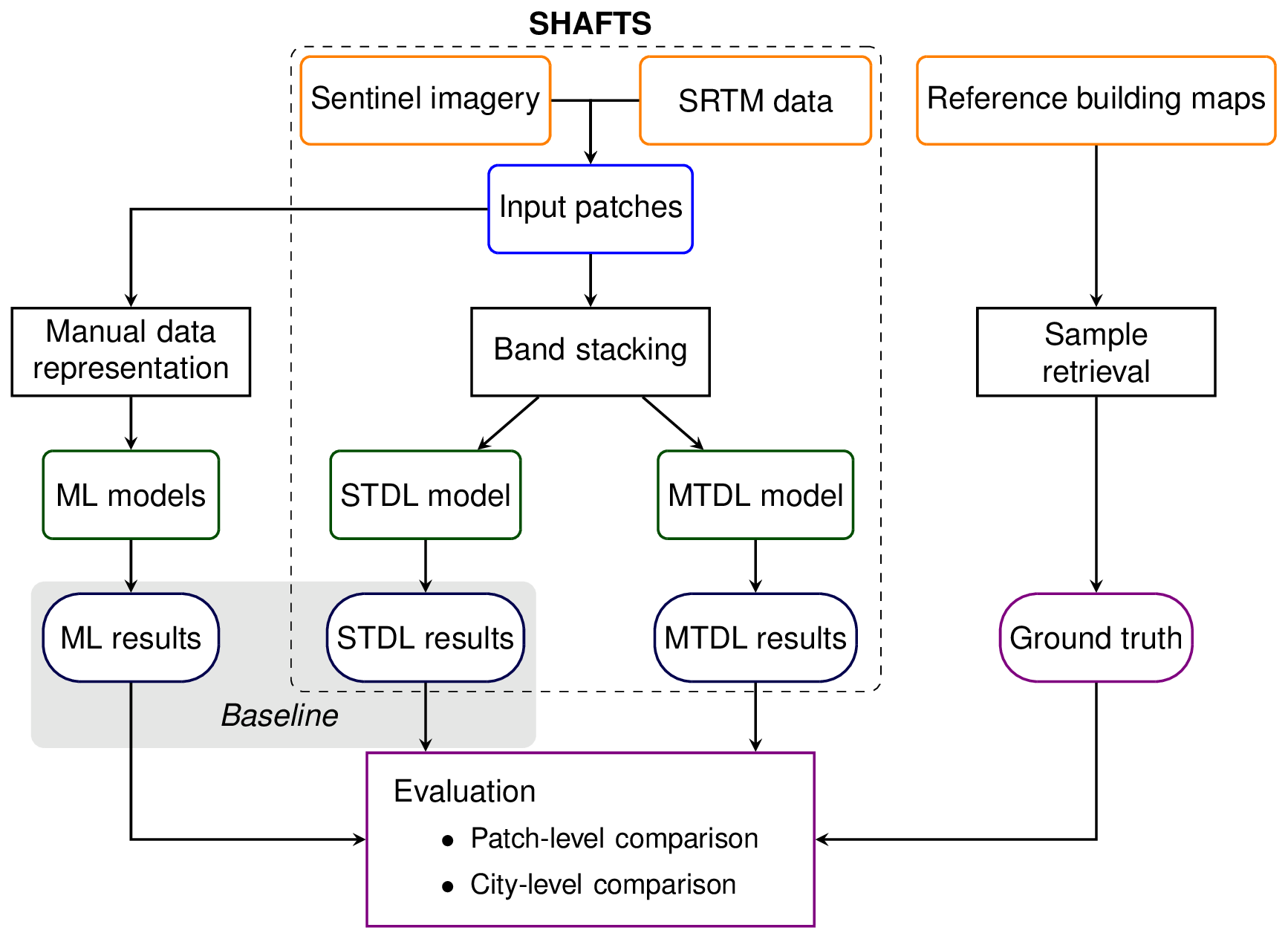
Figure 1Overview of workflows to estimate building height and building footprint using ML and DL approaches.
In the remainder of this paper, we first describe the proposed MTDL approaches for 3D building information extraction (Sect. 2) and then perform diagnostic evaluation of model performance in 46 cities worldwide at both patch and city levels (Sect. 3).
2.1 Theoretical background
For building footprint prediction, optical images are straightforward choices of inputs for most practices (Guo et al., 2021). Also, building height can be estimated from temporal patterns of building shadows which can be detected from time series of optical images (Frantz et al., 2021). However, the quality of optical images is strongly influenced by weather conditions, which leads to research concerning alternative data sources for 3D building information retrieval. Synthetic Aperture Radar (SAR) satellite is one such choice which is capable of all-weather day-and-night imaging (Moreira et al., 2013). SAR images are often displayed in the form of backscattering intensity which heavily depends on the material types, regional distribution and structural shapes of sensed objects (Koppel et al., 2017) and is therefore of great value to 3D building information retrieval. In general, building height estimation from SAR images can be formulated as a problem of inverse modelling: given the radar viewing geometry, underlying 3D building distribution is expected to be inferred from the observed backscattering results. Although radiometric analysis based on SAR models can help to estimate building height in a simulating and matching way (Brunner et al., 2010), complex backscattering mechanisms and unknown prior knowledge about objects such as roof properties and building location constrain the model-based analysis in a real urban context (Sun et al., 2022). Confronted with these challenges, this work proposes to use deep neural networks to learn the solution of the inverse problem in a data-driven fashion. Furthermore, considering that the aforementioned prior knowledge can be derived from optical images and building footprint prediction, this work makes synergistic use of both optical and SAR images and estimates building footprint and height simultaneously.
Additionally, it is worth noting that in order to generate backscattering images for downstream quantitative studies, SAR data processing often requires geometric and radiometric correction on raw images acquired by sensors using a digital elevation model (DEM) (Loew and Mauser, 2007). Thus, the information of DEM can be critical for building height retrieval based on SAR images, especially for areas with variable topography. Although some toolboxes – such as the Sentinel application platform (SNAP) – offer several processing functions to perform such corrections (Piantanida et al., 2021), this work proposes to include the information of DEM as an auxiliary explanatory variable in developed models to envelope terrain-induced effects on backscattering and compensate for possible limitations of existing algorithms.
2.2 Dataset preparation
2.2.1 Explanatory data
Based on the aforementioned theoretical analysis and review of previous practices (Li et al., 2020; Frantz et al., 2021), this work selects the following explanatory data for 3D building information mapping:
-
10 m VV and VH polarizations of Ground Range Detected (GRD) Level-1 products of Sentinel-1 imagery (Torres et al., 2012),
-
10 m red, green, blue and the near-infrared (NIR) band of Level-2A products of Sentinel-2 imagery (Drusch et al., 2012),
-
30 m DEM data from SRTM V3 product.
To construct a convenient engineering pipeline, this work implements functions to download satellite data from GEE through its Python interface, which includes the following steps:
-
Sentinel-1 GRD data acquired in Interferometric Wide-swath (IW) mode, Sentinel-2 Level-2A data with cloud coverage <20 % and SRTM data are retrieved from image collections stored in GEE.
-
All images are filtered by constraints defined by spatial extent and record year derived from corresponding reference data.
-
All bands are aggregated to annual medians for further model development.
It should be emphasized that unlike previous studies (Li et al., 2020; Esch et al., 2022), we do not prescribe urban boundaries as necessary inputs because we deem such information to be inherently encoded in the mapping results and can be extracted automatically by post-processing (Sect. 3.3.2).
2.2.2 Reference data
Based on previous research (Li et al., 2020; Cao and Huang, 2021) and additional searches to our best efforts, we constructed a dataset for 3D building information mapping which consists of 46 cities worldwide (See Sect. S1 in the Supplement for access details). Most reference data used in this work are collected from publicly available sources provided by local governments and the ArcGIS Hub (https://hub.arcgis.com/, last access: 1 November 2022) to allow open research (Nosek et al., 2015). However, considering the inherent noises in open-source datasets due to geo-coordinate offset, measurement error and misreporting (Burke et al., 2021), high-quality cadastral data of London and Glasgow prepared by Digimap (https://digimap.edina.ac.uk/, last access: 1 November 2022) are also included in this work. All reference data are saved as ESRI shapefiles so the building footprint can be calculated from the geometry area and height value can be queried from the attribute table, facilitating the subsequent multi-task learning (MTL) of building footprint and height. We note that although some reference datasets (e.g. Beijing, Chicago) have available information of building floor numbers, the building height is yet to be obtained via conversion with assumed storey heights (Ji and Tang, 2020; Li et al., 2020) that may inevitably introduce bias in building height. Thus, we exclude them from model development but will use them in the later model assessment (Sect. 3.3.1).
The urban surface features high heterogeneity and complex process interactions at various scales (Masson et al., 2020b; Salvadore et al., 2015), which requires researchers to spatially aggregate the per-pixel data at an appropriate scale regarding specific downstream applications (Zhu et al., 2019b). To reveal 3D building characteristics at different scales (100, 250, 500 and 1000 m), average building height Have and building footprint λp (also known as the plan area index) are calculated by fishnet analysis with corresponding target resolutions:
where ℐ is the index set of buildings intersecting with the grid, Ai is the intersection area of the ith building and the pixel, hi is the height of the ith building and r is the target resolution which is equal to the grid spacing of the fishnet layer.
2.2.3 Data preprocessing
For scene-level prediction tasks, input satellite images are partitioned into patches using a moving window centred on the target pixel of the reference data; this facilitates models to ingest the information of surrounding environment. The window moves with a stride equal to the target resolution. Each patch is assigned with corresponding building footprint and height value as prediction targets. Thus, raw dataset 𝒟 for building footprint and height prediction can be constructed as follows:
where s is the patch size (cf. Table 1), 7 is the number of bands used in this work and N is the number of samples.
Based on the preliminary analysis of data records from reference datasets as well as checking rasterized results after the fishnet analysis, we designed several filtering rules for excluding noisy samples from model development:
-
The average building height value should fall into a reasonable interval. According to existing records considering the geolocation of samples, this interval is predefined by the following: .
-
The average building footprint value should be greater than a threshold . Since the footprint value can be calculated based on the summarization of binary classification results at pixel-level, we set the lower bound of model prediction as the area ratio between one pixel and the sample patch, i.e. , with the assumption that deployed models have no access to the sub-grid information.
-
Grids with only few “sliver polygons” during fishnet analysis should be discarded for their inappropriate representation of building bulk properties (Lagacherie et al., 2010). According to Eq. (2), this case often gives rise to a sample patch with an extremely large building height but abnormally small footprint. In this work, we set the corresponding footprint threshold as and the height threshold as 20 m which is close to twice the median of the whole dataset.
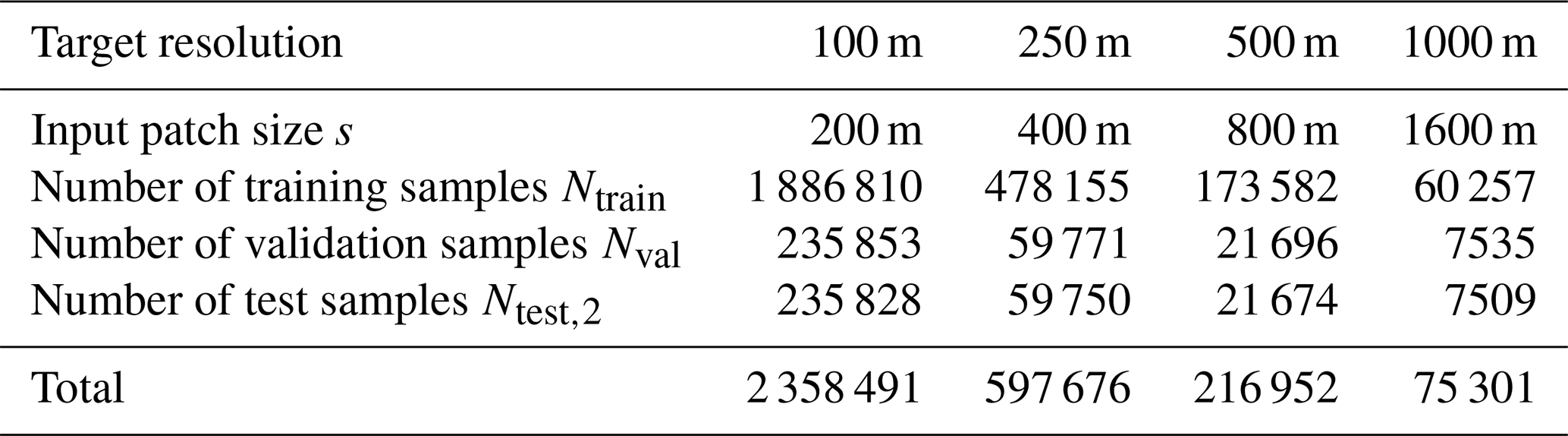
After sample selection, the whole dataset 𝒟 is split into a training set 𝒟train, a validation set 𝒟val and a test set 𝒟test using a two-step selection with different granularity. The first step is city-level selection. Three cities, Beijing, Chicago, Glasgow, are left out as the first part of the test set denoted as 𝒟test,1. The second step is patch-level selection. To be specific, patches from the remaining 43 cities are randomly collected into 𝒟train (80 %), 𝒟val (10 %) and the second part of the test set denoted as 𝒟test,2 (10 %) city by city. The patch-level sampling results under different target resolutions are summarized in Table 1.
Table 1Input sample patch size and number of samples under different target resolutions.
In this work, both 𝒟train and 𝒟val are designed for model training. With regard to performance evaluation, 𝒟test,1 is prepared for testing the spatial transferability of selected models because the surface information and satellite images of these cities are entirely unseen by models during training. The second part of the test set, 𝒟test,2, is designed to investigate the performance difference between ML models and DL models and inform of better models for spatial transferability testing on 𝒟test,1. We note that although a more rigorous procedure with 𝒟val for hyperparameter fine-tuning may further optimize model performance, no further selection of hyperparameters is carried out as this work is not aimed at establishing a new benchmark for certain datasets.
2.2.4 Dataset overview
The reference distributions of Have and λp of 46 cities in the reference dataset are shown in Fig. 2. According to reference distributions of Have and λp, the majority of selected urban patches have a building footprint value ranging from 0.0 to 0.3 and height value ranging from 3 to 40 m. Furthermore, the comparison of reference distributions under different target resolutions reveals negligible effects of spatial resolution on the typical distribution of Have but strong influence on λp: when the target resolution decreases from 100 to 1000 m, the median of λp decreases from 0.13 to 0.008 while the median of Have merely decreases from 8.7 to 8.1 m. Also, the inter-quartile range (IQR) of Have remains about 8.6 m under different resolutions while that of λp decreases from 0.17 to 0.08. Such an effect of spatial resolution indicates that surface heterogeneity is more vertically prominent: when spatial resolution comes close to the critical point satisfying homogeneous surface assumption with respect to λp, it would still be far from that of Have, so the distribution of Have remains nearly unchanged.

Figure 2Top: Sentinel's images of five representative cities where band values are shown in their annual medians and reference building layers are overlaid on the R/G/B bands of Sentinel-2's images. Bottom: reference distributions of Have and λp in 46 individual cities and overall dataset 𝒟 where each pair of vertical and horizontal lines are characterized by upper, lower bounds and middle points which represent the quartiles of the distributions of Have and λp, respectively.
We select five cities as representatives – Prince George (Canada), London (UK), San Francisco (USA), Chattanooga (USA) and Porirua (New Zealand) – that roughly lie on the boundary of urban clusters and present their Sentinel images in Fig. 2. They are located in different continents and exhibit various semantic categories: sparsely built middle risers in Porirua, open low risers in Prince George, open high risers in Chattanooga and compact low risers in London and San Francisco. Based on visual interpretation, although the limited resolution of Sentinel-2's images might hinder us from identifying buildings in over-bright or shadow regions with high confidence, most building footprints coincide well with corresponding polygons in reference building layers spatially, which demonstrates the reliability of reference datasets.
2.3 Model description
2.3.1 Architecture of the CNN model
The CNN models commonly consist of powerful backbones for hierarchical feature extraction and some heads for specific downstream tasks such as classification and regression. We adopt a residual neural network (ResNet) (He et al., 2016) integrated with Squeeze-and-Excitation (SE) blocks (Hu et al., 2018) as our backbone model denoted as SENet (Fig. 3). Compared with prior architectures such as VGG (Simonyan and Zisserman, 2015) and Inception (Szegedy et al., 2015), ResNet adopts the framework of residual learning and inserts shortcut connections into the plain neural networks; this eases the training of much deeper models without degradation of performance (He et al., 2016). After the proposal of ResNet, various strategies have been introduced to further improve its performance in computer vision tasks. One of the mainstream approaches is the visual attention mechanism which assigns adaptive importance weights to each channel or spatial position for higher emphasis on critical input elements (Qin et al., 2021; Zhu et al., 2019a). In this work, we use SE blocks within ResNet where channel-wise attention is calculated by two fully connected (FC) layers after the global average pooling (GAP) on the input feature maps. In each SE block, the GAP produces an embedding of global spatial information for individual channels and the subsequent FC layers capture interdependencies between channels based on the embedding so that per-channel modulation weights can be generated (Hu et al., 2018).
Furthermore, compared with standard practices in similar tasks using Sentinel imagery (Frantz et al., 2021; Geiß et al., 2020), we take the potential influence of local terrain relief on 3D building information mapping into consideration. Considering that DEM is a relatively static dataset when compared with Sentinel imagery, we design another input branch of SRTM to allow the potential capacity of our proposed CNN models in learning-distinct temporal dynamics of different characteristics separately. After feature extraction is performed by individual backbones, two branches are merged by concatenating feature information from both Sentinel imagery and SRTM. Preliminary experiments show much improvement brought by the introduction of DEM information in building height prediction, especially at refined scales such as 100 m. See Sect. S2 for access details.
For simplicity, we use two FC layers in head design. The choice of final activation function depends on the target variable where the sigmoid function is used for building footprint prediction and a rectified linear unit (ReLU) function is used for building height prediction.
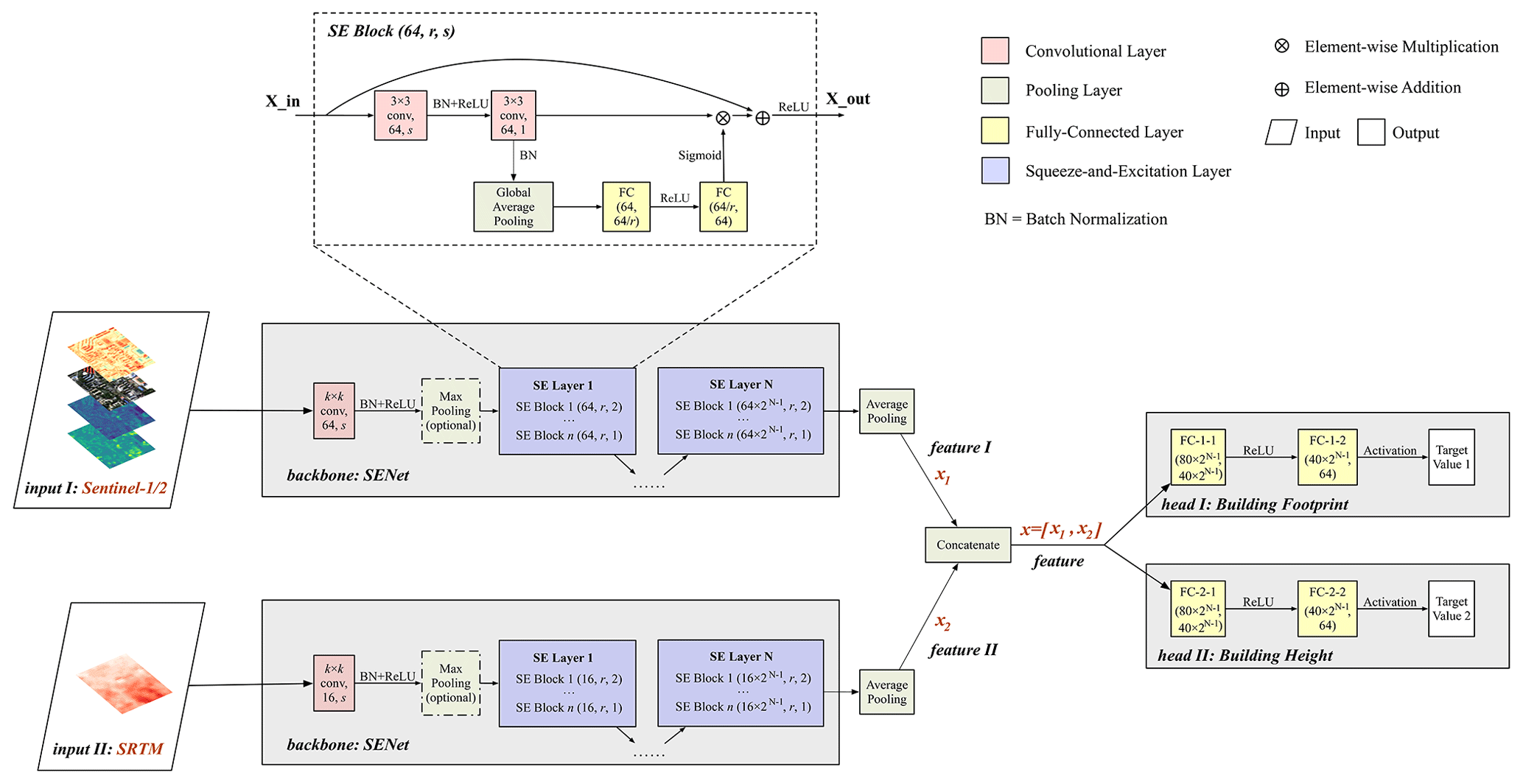
Figure 3The architecture of the CNN deployed in this work. The convolutional layer is parameterized by k×k conv, c, s, where k is the kernel size, c is the number of output channels and s is the stride. For initial convolution used in the backbone part, k=3, s=1 is chosen for the cases of 100 m and k=7, s=2 is chosen for the cases of 250, 500 and 1000 m. The max-pooling layer is only used for the cases of 500 and 1000 m. The fully connected layer is parameterized by Din, Dout, where Din is the input dimension and Dout is the output dimension. The SE block part is parameterized by Cin, r, s, where Cin is the number of input channels, r is a reduction ratio (Hu et al., 2018) for the fully connected layer (r=16 in this work) and s is the stride of convolution. The number of SE layers denoted by N is chosen as 4 for the case of 1000 m and 3 for other cases (for the case of 100 m, the stride of the first SE block in the first SE layer is chosen as 1). The number of SE blocks in each SE layer denoted by n is chosen as 1 for all cases.
2.3.2 Multi-task learning
Multi-task learning (MTL) aims to improve learning for one task using the information enveloped in the training signals of other related tasks (Caruana, 1997). Compared with single-task learning (STL), MTL features higher learning efficiency as well as less over-fitting risk since it guides models to reach more general feature representation preferred by multiple related tasks, which can be considered as an inductive bias for the regularization of deep neural networks (Ruder, 2017). One of the common practices of MTL is to carry out multiple tasks simultaneously through the minimization of a weighted sum of individual losses (Eigen and Fergus, 2015). According to Fig. 3, we formulate the MTL loss L as follows:
where and are the loss functions of footprint and height prediction tasks, respectively.
While loss weights w1 and w2 can be fixed as constants during the training, several dynamic weighting schemes have been proposed based on task uncertainty (Cipolla et al., 2018), gradient norm (Chen et al., 2018) or Pareto optimality (Sener and Koltun, 2018). In this work, we adopt two weighting schemes during model development:
-
Dynamic weight scheme is based on task uncertainty (Cipolla et al., 2018; Liebel et al., 2020) where the loss function for MTL is reformulated as
where and are uncertainty measures for corresponding tasks which can be treated as trainable parameters along with the parameters of CNN. In practice, instead of and , their log values, i.e. and , are optimized to improve numerical stability.
-
In the fixed weight scheme, the fixed weight ratio is chosen based on preliminary results of the dynamic weight scheme with w1=100 and w2=1. See Sect. S3 for access details.
To investigate the effects of MTL, we additionally train the CNN in the STL mode by using only one branch of the heads. For notational simplicity, we do not differentiate two weighting schemes hereafter and refer to CNNs trained by MTL with better overall performance on 𝒟val as MTDL models, CNNs trained by STL as STDL models.
2.3.3 Loss function
Mean squared error loss (MSELoss) has been commonly selected as the loss function for the task of regression, which is defined as follows:
where is the predicted value and y is the reference value.
However, MSE places much more emphasis on samples with large absolute residuals during the fitting process and may thus result in a far less robust estimator when applied to grossly mismeasured data (Hastie et al., 2009). Therefore, other metrics such as mean absolute error (MAE) and their combinations are adopted for model training on noisy data. In this work, we use the adaptive Huber loss (AHL) defined by (Huber, 1964):
where δ is a threshold that represents the estimated regression residual caused by potential outliers.
The AHL avoids some undesired optimization issues caused by the constant norm of the gradient of MAE and is also less sensitive to the outliers when compared with MSE. However, the choice of δ becomes another concern for its implementation. In this work, we initialize δ by the normalized median absolute deviation (NMAD) of the training dataset (Hastie et al., 2009) which is defined by
where j is traversed from 1 to Ntrain and q50 is the 50th percentile operator. Then δ is adjusted adaptively during the training process using the following equation:
where i is the number of finished epochs and q90 is the 90th percentile operator.
2.3.4 Data augmentation
Multiple factors including light scattering mechanisms, atmospheric scattering conditions and equipped device health can bring non-negligible uncertainty and noise to the acquired satellite imagery which presents a great challenge to the generalization ability of deep networks applied to a global scale (Zhu et al., 2017). While assembling adequate data can tackle this problem from its root, it might be a daunting task due to the collection difficulty and computational cost. Instead of inflating the dataset directly, data augmentation uses data warping or oversampling during the training process to help deep networks in efficiently learning certain translational invariances (Shorten and Khoshgoftaar, 2019). In this work, we employ the data-warping strategy that randomly transforms the sample patch by flipping, colour space shifting and noise injection while preserving the target value. To be specific, to mimic various noises during image acquisition, we add the Gaussian noise to Sentinel-1's VV, VH bands and Sentinel-2's NIR band; we then add the ISO noise, Gaussian noise and colour jittering to Sentinel-2's red, green and blue bands, where transformation probabilities for each operation are all set to 0.5. Finally, after stacking all bands including the DEM band, we randomly flip the multi-spectral sample patch with a probability of 0.5.
2.4 Technical implementation
The above-designed DL models are implemented using PyTorch (https://pytorch.org/, last access: 1 November 2022). To achieve faster convergence, we adopt the cosine annealing with warm restarts (Loshchilov and Hutter, 2017) as our learning rate scheduler. To be specific, we choose the initial learning rate lr(0) as 0.01 and then decrease it following a cosine curve:
where lr(i) denotes the learning rate at the ith epoch, Tcur,t the number of epochs since the tth restart and Tt the number of epochs between the tth and t+1th restart. In this work, we trained CNNs for 155 epoches with T0=5, T1=10, T2=20, T3=40 and T4=80.
For optimizer selection, we use the Stochastic gradient descent (SGD) optimizer for single-task learning and the Adam optimizer for multi-task learning. The momentum factor of SGD optimizer is set to 0.9.
Running averages of the gradient and its square of the Adam optimizer are set to 0.9 and 0.999, respectively.
The weight decay factor of both optimizers is set to 0.0001.
Batch sizes used for gradient estimation is set to 64 (256) when STL (MTL) is chosen.
Pre-trained parameters are saved into PyTorch state_dict objects which can be further loaded by the torch.nn.Module.load_state_dict function.
The implemented pipeline has been published as an open source Python package, SHAFTS (Simultaneous building Height And FootprinT extraction from Sentinel imagery), and its source code is available at https://github.com/LllC-mmd/3DBuildingInfoMap (last access: 1 November 2022).
SHAFTS includes the following key functions:
-
sentinel1_download_by_extent– download Sentinel-1's images from GEE according to the specified year, spatial extent and temporal aggregation, -
sentinel2_download_by_extent– download Sentinel-2's images from GEE according to the specified year, spatial extent and temporal aggregation, -
srtm_download_by_extent– download SRTM data from GEE according to the specified spatial extent, -
pred_height_from_tiff_DL_patch– predict building height and footprint using the STDL model, -
pred_height_from_tiff_DL_patch_MTL– predict building height and footprint using the MTDL model.
For detailed usage of these functions, refer to the home page of SHAFTS (https://github.com/LllC-mmd/3DBuildingInfoMap, last access: 1 November 2022).
3.1 Baseline models and evaluation metrics
Based on the review of related work (Li et al., 2020; Frantz et al., 2021), we select RFR, SVR and its bagging version (BaggingSVR), and XGBoostR (Chen and Guestrin, 2016) as ML baselines for comparison with DL models. See Appendix A for implementation details of ML approaches. Also, STDL models are developed as benchmarks to investigate the effects of MTL.
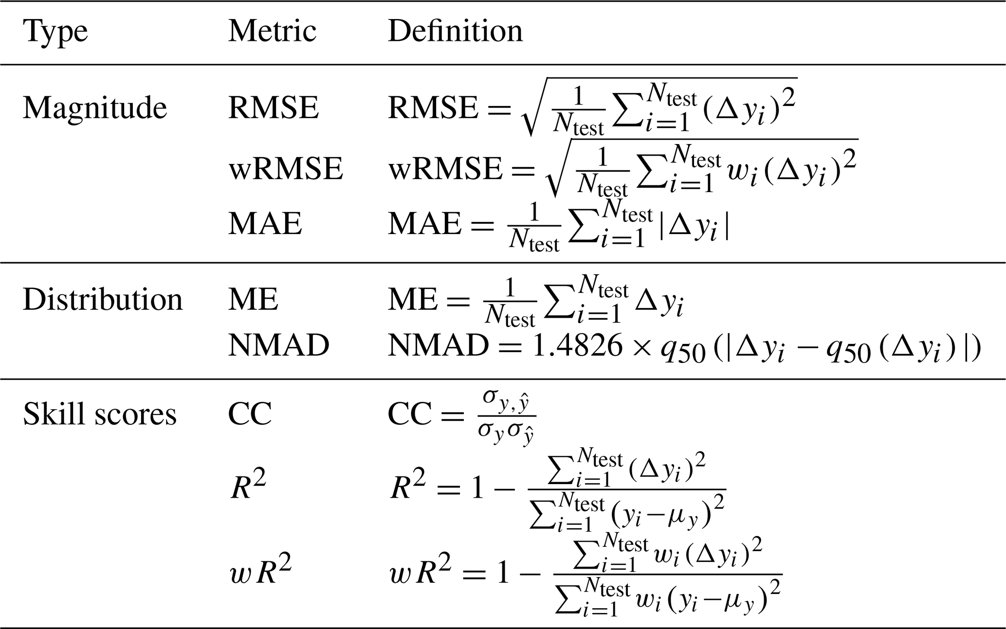
To give quantitative assessment to the performance of our developed models, experimental results are evaluated on 𝒟test using multiple metrics including RMSE and its weighted version (wRMSE), MAE, ME, NMAD, Pearson correlation coefficient (CC), coefficient of determination (R2) and its weighted version (wR2) defined in Table 2.
Table 2Summary of metrics used in this work: y and stand for reference value and predicted value, respectively; . μy is the sample mean of y; σy and are the sample standard deviations of y and , respectively; σy and is the sample covariance between y and , respectively; wi is the weight of regression residual determined by the frequency of corresponding target value which can be estimated using Gaussian kernel density estimation.
Before we embark on the specific results of model evaluation, it is worth reflecting on the incentives for the selection of these metrics.
For the magnitude of model error, RMSE and MAE are common measures using the L2 and L1 norm. Compared with MAE, RMSE can be sensitive to the performance degradation of models caused by outliers such as skyscrapers which may be scarce in the real urban environment. Thus, Frantz et al. (2021) proposed using RMSE weighted by the sample frequency (wRMSE) as a measure of the areal accuracy of models. Besides the magnitude, both centre location and dispersion are key aspects of error distribution, which can be described by ME and NMAD, respectively. The selection of NMAD instead of the sample standard deviation is because the former is considered to be a more robust estimator for the standard deviation than the latter (Carrera-Hernández, 2021).
Furthermore, since the distribution of the target dataset may vary significantly across scales, some dimensionless normalized metrics are preferred for the convenience of intercomparison in relative terms. The Pearson correlation coefficient (CC) is widely used as an overall skill score for assessing structural similarity (Li et al., 2020; Taylor, 2001). A higher CC suggests a more consistent tendency in variation between reference and prediction if any linear transformation is allowed. However, since linear transformation may discard the information about the centre location and amplitude of error distribution, R2 is further selected to provide the complementary information quantifying the overall model performance. Originally, R2 indicates the percentage of target variance explained by a linear regression model. It can be further extended to the nonlinear case to reflect the improvement over the benchmark model if the mean target value is thought to be an appropriate choice (Schaefli and Gupta, 2007). Thus, for representation of urban morphology, R2 can be interpreted as a skill metric which quantifies the performance improvement or degradation of models in capturing surface heterogeneity relative to homogeneous approximation using the sample mean.
3.2 Patch-level evaluation of prediction skill
3.2.1 Performance overview
For building height prediction, as shown in Fig. 4, ML models achieve RMSE ranging from 9.46 to 6.85 m and R2 varying from 0.173 to 0.455, while DL models achieve RMSE ranging from 5.26 to 3.95 m and R2 varying from 0.718 to 0.818. The performance gaps between ML models and DL models are narrowed if we use wRMSE and wR2 for the overall assessment. However, wRMSE measures are still reduced by 0.49 to 1.76 m when comparing DL models with ML models, which is equivalent to nearly 27 %–61 % reduction in the overall error of ML models. Thus, DL models show significant overall performance improvement over ML models. Furthermore, DL models give more robust estimations since they achieve much smaller error variance than ML models for all cases in terms of NMAD. Among ML models, RFR shows the poorest performance and is inclined to over-smoothing which overestimates low height value and underestimates high height value. Additionally, SVR exhibits the best capability of height prediction among the three ML models which agrees with the results of previous research (Frantz et al., 2021).
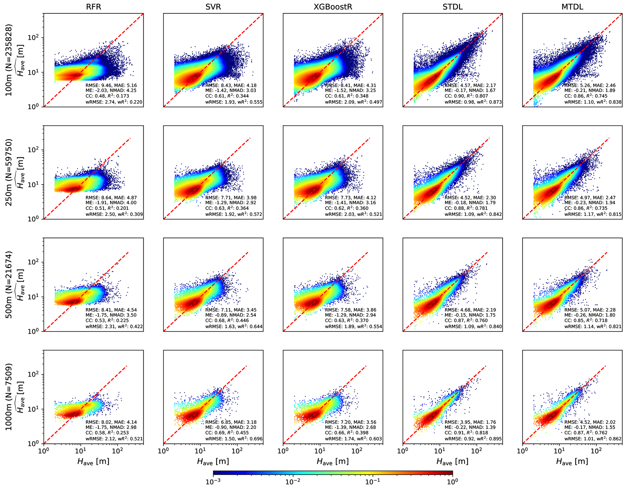
Figure 4Have predicted by ML models and DL models. The density of scatter points is normalized to [10−3, 1] and represented using shading colours. The presented evaluation metrics are calculated based on the reference values from 𝒟test,2 which consists of samples from 43 cities by patch-level sampling (See Sect. 2.2.3 for details).
For building footprint prediction, as shown in Fig. 5, ML models achieve R2 ranging from 0.377 to 0.846 and DL models achieve R2 varying from 0.834 to 0.972. Thus, when compared with building height prediction, overall performance gaps between ML models and DL models of building footprint prediction are much smaller. For most developed models, except for RFR, when the target resolution decreases, area with high density rotates gradually and results in a more symmetric and concentrated distribution on the left and right of the one-to-one line. This tendency of area with high density would make the slope closer to 1.0 when regressing the reference against the predicted values which indicates the improvement of performance measured by the quotient of CC divided by (Gupta et al., 2009).
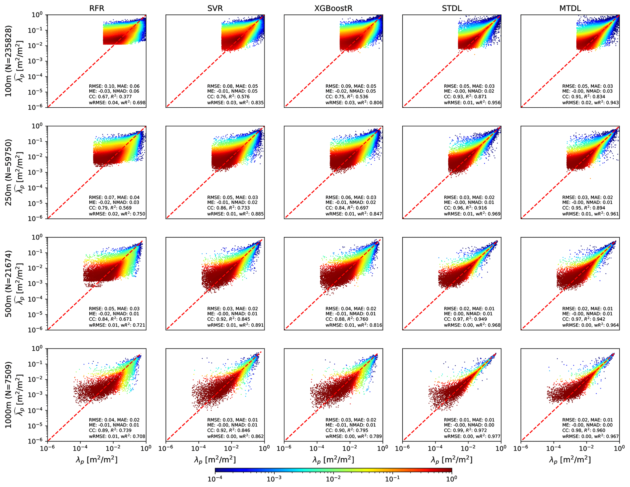
Figure 5λp predicted by ML models and DL models. The density of scatter points is normalized to [10−4, 1] and represented using shading colours. The presented evaluation metrics are calculated based on the reference values from 𝒟test,2 which consists of samples from 43 cities by patch-level sampling (See Sect. 2.2.3 for details).
3.2.2 Stratified error assessment
To further investigate the model performance in certain target domains, we conducted a stratified error assessment in two steps. We first split the original dataset 𝒟test,2 into combinations of different subsets of reference Have and λp. Then, we calculated RMSE, ME and NMAD over each sub-dataset. The summary of error metrics is presented in Figs. 6 and 7.

Figure 6Error metrics of building height prediction in different target domains. Only results from SVR are presented since it achieves the best performance among the three ML models.
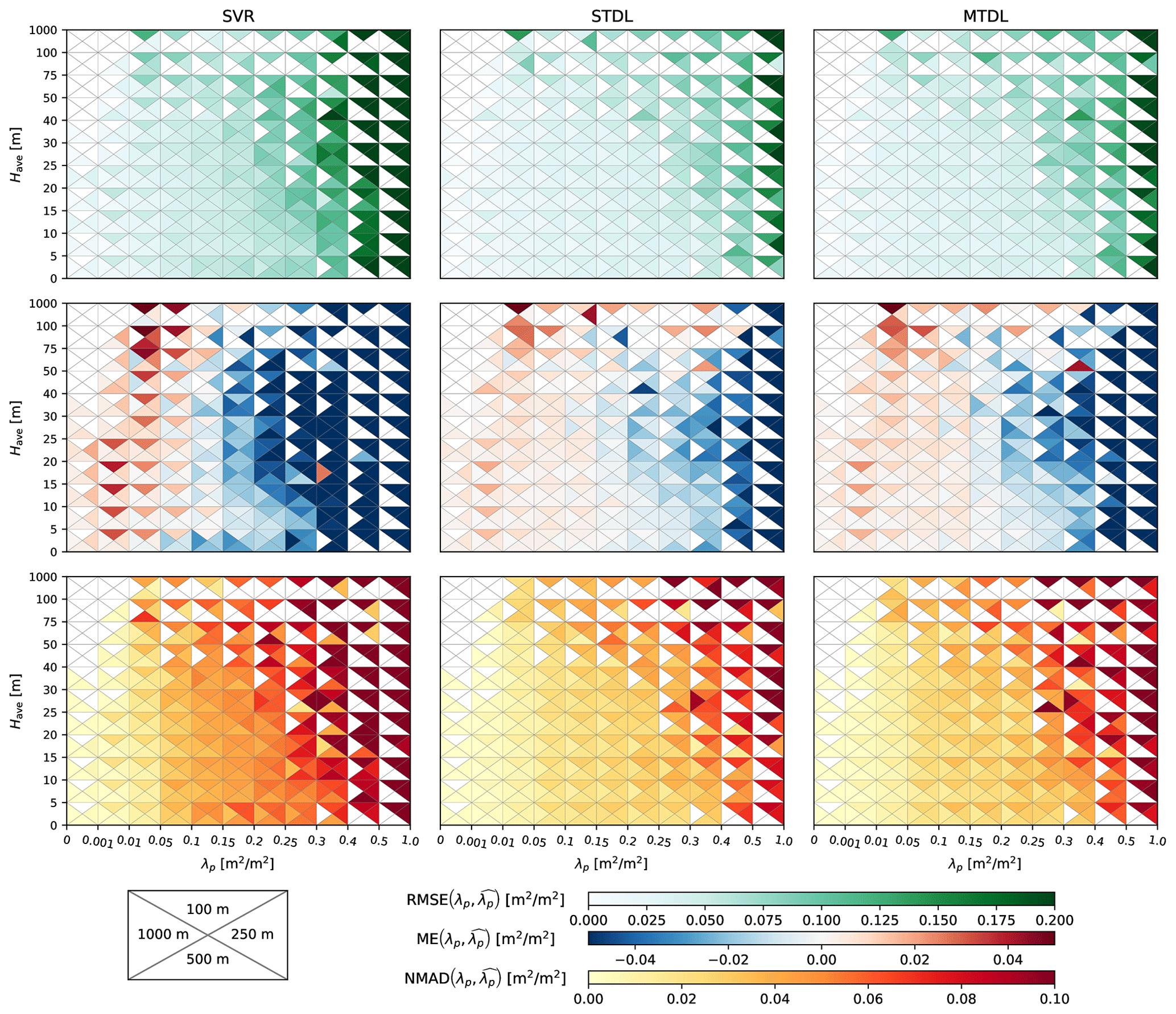
For building height prediction in different target domains, SVR shows large systematic underestimation for Have above 20 m in all cases, which is recognized as the saturation effect in previous research (Frantz et al., 2021; Koppel et al., 2017). In contrast to SVR, both STDL and MTDL models exhibit greatly mitigated saturation effects for the prediction of Have ranging from 20 to 40 m, indicating the suitability of DL models for the prediction of high risers. However, average systematic underestimation of Have above 40 m can still be −18.3 m for STDL models, −28.5 m for MTDL models in the case of 100 m, which might result from the scarcity of samples whose average building height is higher than 40 m (cf. Fig. 2). Besides improving high-riser prediction, when compared with SVR, DL models also reduce the average systematic overestimation of building height lower than 5 m by 42 %–70 % based on the statistics of all cases. A similar phenomenon of systematic underestimation exists when SVR makes predictions on target λp larger than 0.25 where DL models achieve 61 %–81 % reduction on ME. Also, both SVR and DL models tend to overestimate the target λp smaller than 0.05, especially in the case of 100 m. This might be largely attributed to the limited resolution of Sentinel's imagery where small buildings in a low-density built-up area can not be clearly resolved. The problem of systematic overestimation is mitigated when target resolution becomes coarser since more information from the surrounding environment can be utilized to infer building existence under a medium resolution of 10 m.
Based on the preliminary results of stratified analysis on ME, we further grouped target domains of Have and λp into three representative intervals separately. We also summarized the average error magnitude measured by RMSE and standard deviation of error measured by NMAD over these intervals in Fig. 8. See Sect. S4 for detailed quantification results of model performance. Both SVR and DL models show lower RMSE and NMAD for the low-value domain compared with other domains, which, however, should be interpreted with the consideration of data ranges of respective domains – relatively unfavourable model performance may be observed for the low-value domain if quantified with RMSE/NMAD normalized by domain-specific reference values (e.g. medians). When it comes to medium-value domain where the majority of samples lie (cf. Fig. 2), for building height prediction, DL models reduce RMSE and NMAD by 2–3 and 0.4–1.5 m, respectively, when compared with SVR. For building footprint prediction in the medium-value domain, performance improvement brought by DL models tends to increase with the coarsening of target resolution. Such a phenomenon indicates that building footprint prediction can benefit more from the growing size of input patches when compared with building height prediction. For the high-value domain, although both error magnitude and standard deviation of error become much larger, it can be naturally attributed to the increasing dynamic range of target values (Geiß et al., 2019). Furthermore, when compared with SVR in the high-value domain, DL models reduce RMSE by 31 %–50 % for building height prediction and 40 %–67 % for building footprint prediction, which demonstrates the superiority of DL models on the 3D building information prediction in target domains with high Have and λp.

Figure 8RMSE and NMAD of building height and footprint prediction over representative intervals where NMAD corresponds to half the length of error bars distributed symmetrically at the ends of boxes. For building height prediction, the low-value, medium-value and high-value domains are defined by Have<5 m, 5 m m, 40 m m, respectively. For building footprint prediction, the low-value, medium-value and high-value domains are defined by λp<0.05, , , respectively.
Furthermore, Fig. 7 reveals the dependence between error metrics of building footprint prediction and target building height: larger error magnitude and uncertainty of building footprint prediction can be noticed for domains with higher building height. It might be caused by the layover and shadow effect brought by high risers on surrounding environment which hinders models from capturing all existing building footprints precisely (Stilla et al., 2003).
3.2.3 Diagnosing performance gaps between DL and ML models
To further investigate why the DL models outperform the ML ones, we conducted a decomposition analysis of R2 (Fig. 9).
Intuitively, an appropriate prediction requires both magnitude and variability of the underlying distribution to be captured accurately. Following this insight, a causal link can be drawn among proposed error metrics to promote the model evaluation towards a more diagnostic sense. Using normalization, 1−R2 can be related with RMSE (Gupta et al., 2009) and then decomposed into the summation of the magnitude part measured by ME and the variability part measured by centred RMSE (Taylor, 2001):
where RMSE′ is the centred RMSE defined by
where is the sample mean of .
Basically, Eq. (11) indicates that variation in model performance measured by R2 (or RMSE) consists of systematic deviation from the centre quantified by ME and associated variability measured by RMSE′. Since systematic deviation represented by ME is easier to correct, more emphasis can be laid on the analysis of the variability error measured by RMSE′.
Taylor (2001) gives a decomposition of RMSE′ following the form of the law of cosines:
Equation (13) suggests that RMSE′ is influenced by variability consistency quantified by CC and variability magnitude quantified by . The similarity between this decomposition formula and the law of cosines facilitates the model comparison by a single intuitive image called the Taylor diagram (Taylor, 2001).
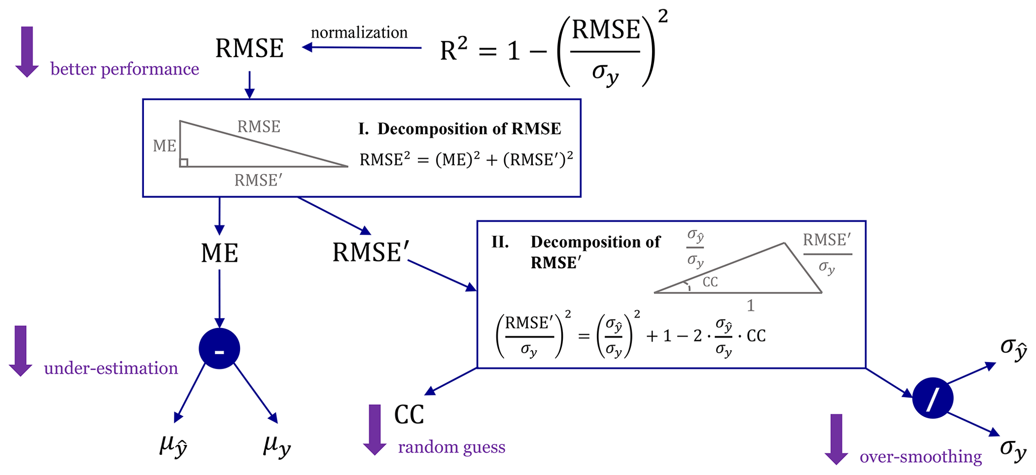
Figure 9Decomposition of RMSE and R2 where two boxes represent two steps of the decomposition analysis. Coloured arrows indicate the computation flow for error metrics and coloured circles represent the computation operators where “–” denotes and “/” denotes . See Table 2 for detailed definitions of symbols.
According to Fig. 9, we first decompose 1−R2 into the summation of a systematic bias MEn and a variability error . We then find that the variability error (i.e. ) dominates the variation of 1−R2 (Fig. 10) and is about 50 % smaller in DL models than in ML ones. Furthermore, of building height and footprint prediction mainly shows a decreasing trend when target resolution becomes coarser which indicates the improvement of model skills on capturing variability. For all cases, only accounts for a small fraction of 1−R2: it can be largely ignored in DL models but stays at a quasi-constant non-negligible level in ML ones, especially for building height prediction. Such decomposition suggests that, when compared with ML models, the significant improvement brought by DL models are mainly due to considerable reduction in variability errors. However, it is also remarkable that for ML models, owing to almost an invariant level of systematic bias, it can be expected to occupy a much larger percentage of total error when target resolution becomes coarser.

Since the variability error dominates the overall bias, we further attribute the variation of to the magnitude part measured by and the consistency part measured by CC (Fig. 11).
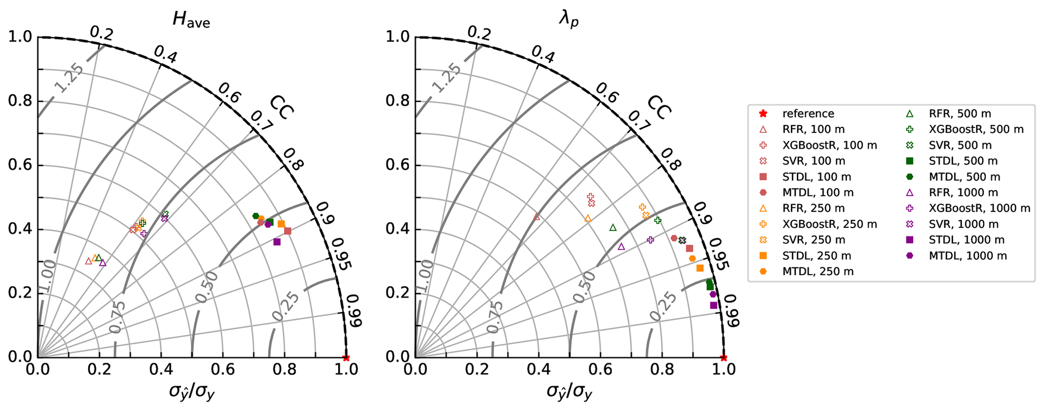
Figure 11Taylor plots of comparing model performance across different scales where contours represent different levels of .
For building height prediction, CC of ML models mainly vary between 0.48 and 0.69, which indicates the moderate correlation between reference and prediction. And DL models further improve the results of CC by 0.17 to 0.42. Besides, a larger magnitude (0.22–0.56) of difference in can be found between ML and DL models. Therefore, the better performance of DL models over ML ones can be mainly attributed to the improvement of variability magnitude.
However, for building footprint prediction, the variation of model performance seems to be more complicated. This phenomenon might result from the mixture effects of model and dataset. Reference height distribution shows minimal variability when the resolution changes from 100 to 1000 m (Fig. 2) and thus largely reduces the influence caused by distribution transformation. However, improvement brought by DL models in both CC and can still manifest (Fig. 11), though the magnitude of improvement becomes less remarkable when compared with building height prediction. The narrowed performance difference between DL and ML models also agrees with the comparison results with respect to overall performance on Have and λp (Sect. 3.2.1).
3.2.4 The effects of MTL
For patch-level evaluation, STDL models achieve better performance than MTDL ones (Figs. 10 and 11). However, the performance gap between STDL and MTDL models narrows when target resolution becomes coarser (Fig. 10). This is probably due to more contextual information gradually ingested by larger input patches. When target resolution decreases from 100 to 1000 m, input size increases from 200 to 1600 m and thus more contextual information about the surrounding environment – such as the spatial distribution of surface elevation, land cover and building shadows – can be utilized to extract features, which can benefit downstream inference tasks (Mottaghi et al., 2014). This can be further evidenced by t-SNE visualization (van der Maaten and Hinton, 2011) of features extracted by the backbone part of DL models (Fig. 12): for building height prediction, when compared with manually constructed features for ML models, automatically learned features of DL models gradually separate sample points with different magnitude of height values into several groups when target resolution decreases, indicating features with more discriminative power are learned by DL models.
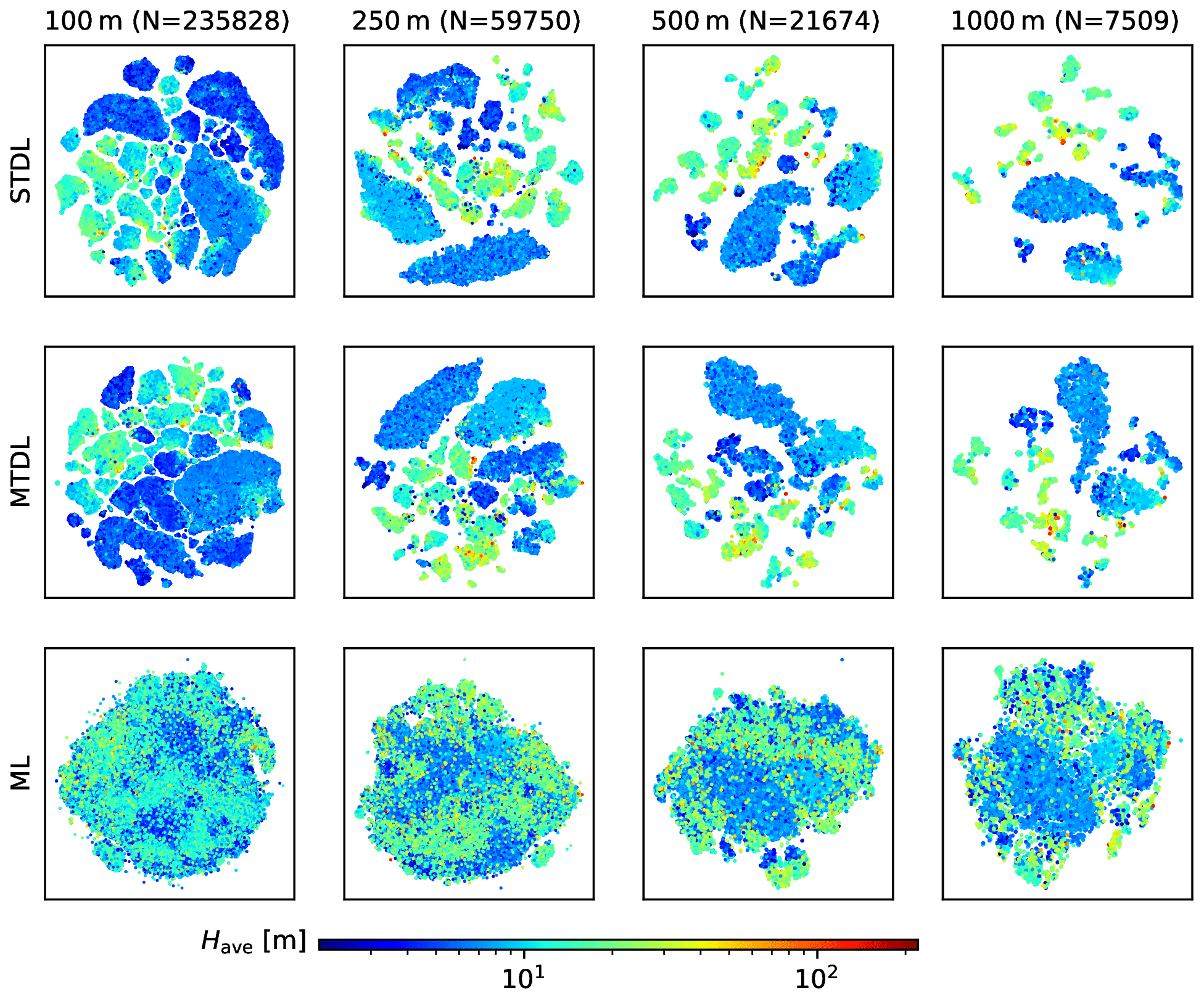
Figure 12Visualization of features for building height prediction in 𝒟test,2 using t-SNE. Features of STDL and MTDL models are defined as the output from the backbone part while features of ML models are extracted using techniques mentioned by Sect. A1.
Compared with STDL models, although MTDL models exhibit different learned feature patterns due to the fact that they are trained using two branches of the heads (See Sect. 2.3.2 for details), they can achieve comparable performance (consistent with a previous pixel-level result of Cao and Huang, 2021). Also, MTDL models are more efficient as evidenced by nearly halving the number of parameters compared to STDL ones (Table 3). This conclusion can be further confirmed by the t-SNE visualization of features for building footprint prediction (Fig. 13). Transformed distribution of features extracted by MTDL models remains the same for both cases whereas boundaries splitting different types of sample points are still maintained clearly. In contrast, features learned by STDL models exhibit a totally different and more mixed form of distribution compared with the case of building height prediction. Since both STDL and MTDL models learn the representation of the same dataset, much redundancy can be expected in the learning results of STDL models.
Table 3Summation of the number of parameters for simultaneous building height and footprint prediction using STDL and MTDL models under different target resolutions.
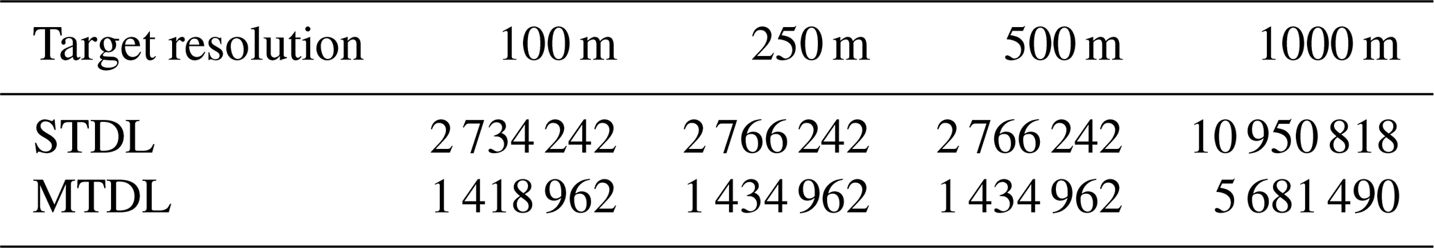
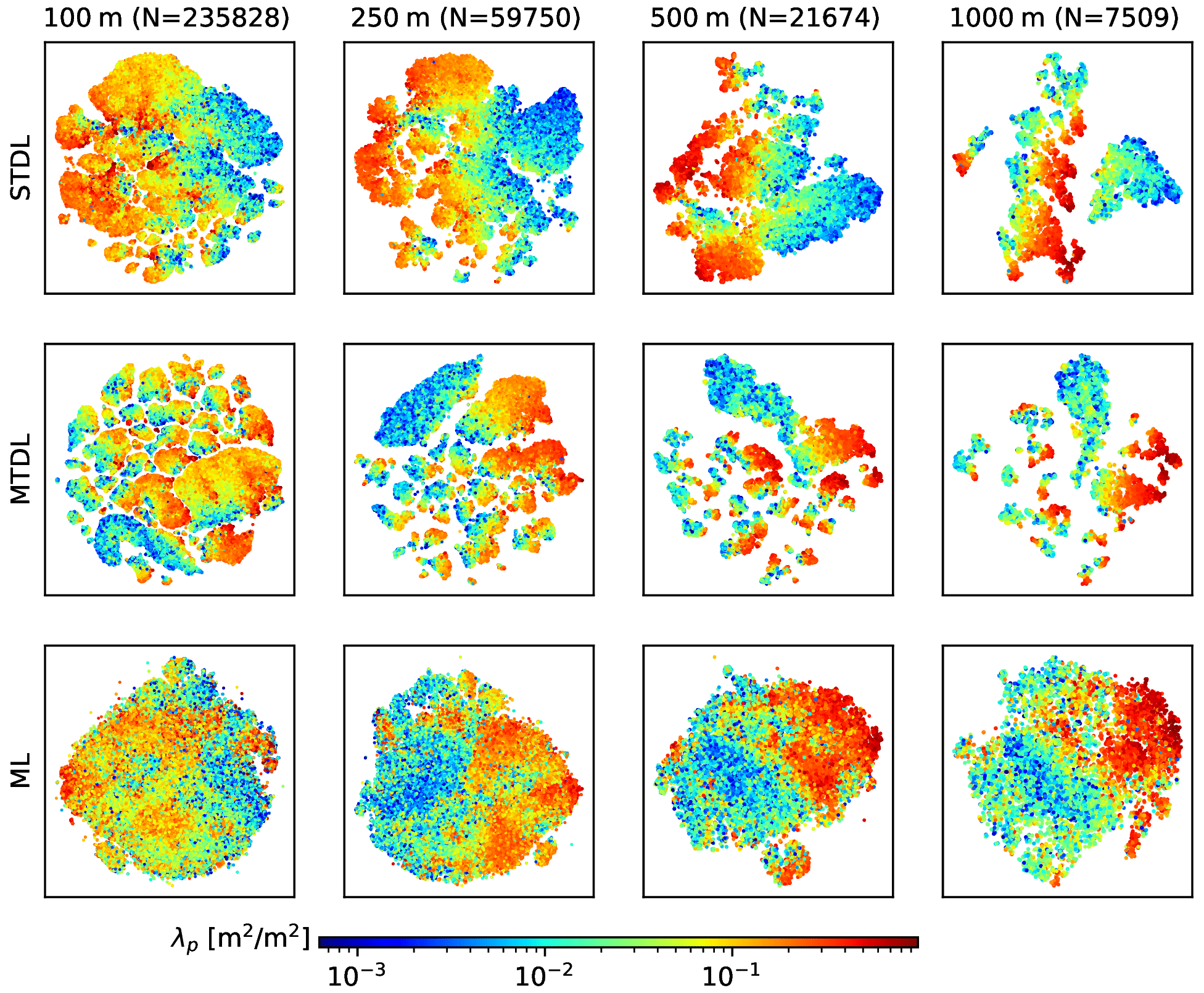
Figure 13Visualization of features for building footprint prediction in 𝒟test,2 using t-SNE.
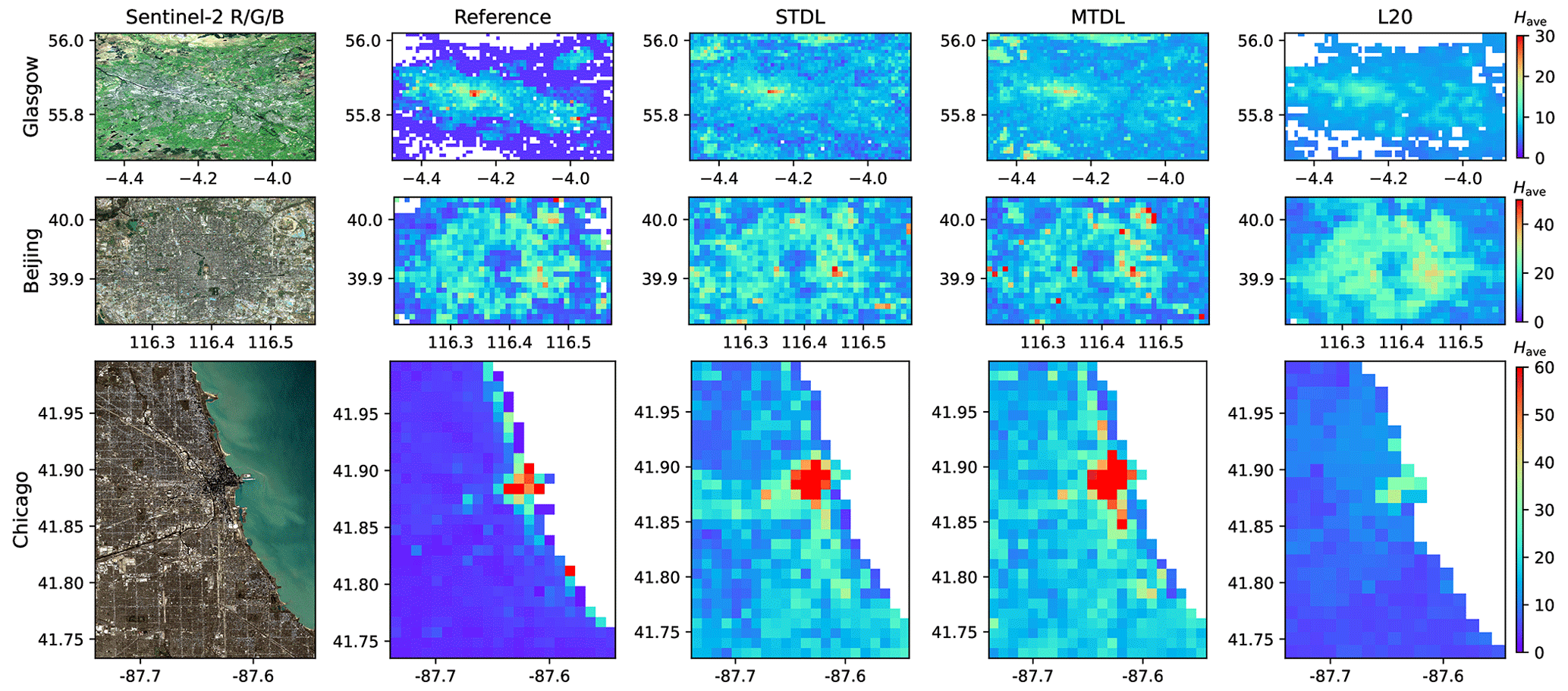
Figure 14Building height close-ups in Glasgow, Beijing and Chicago.
3.3 City-level evaluation of spatial transferability
3.3.1 Qualitative evaluation in Glasgow, Beijing and Chicago
To further investigate the spatial transferability of our developed DL models, we mapped 3D building structures at 1000 m resolution for three metropolitan areas from different continents, namely Glasgow, Beijing and Chicago (Figs. 14 and 15). As the height information of Beijing and Chicago is only available as floor numbers, it is converted into building height with an assumed storey height of 3 m following Cao and Huang (2021); Li et al. (2020). Also, we compare our results against a recent 3D mapping product based on RFR (Li et al., 2020; L20 hereinafter), which utilizes multi-source data including remote-sensing imagery and additional information including urban footprint mask and roads (Cao and Huang, 2021; Frantz et al., 2021).
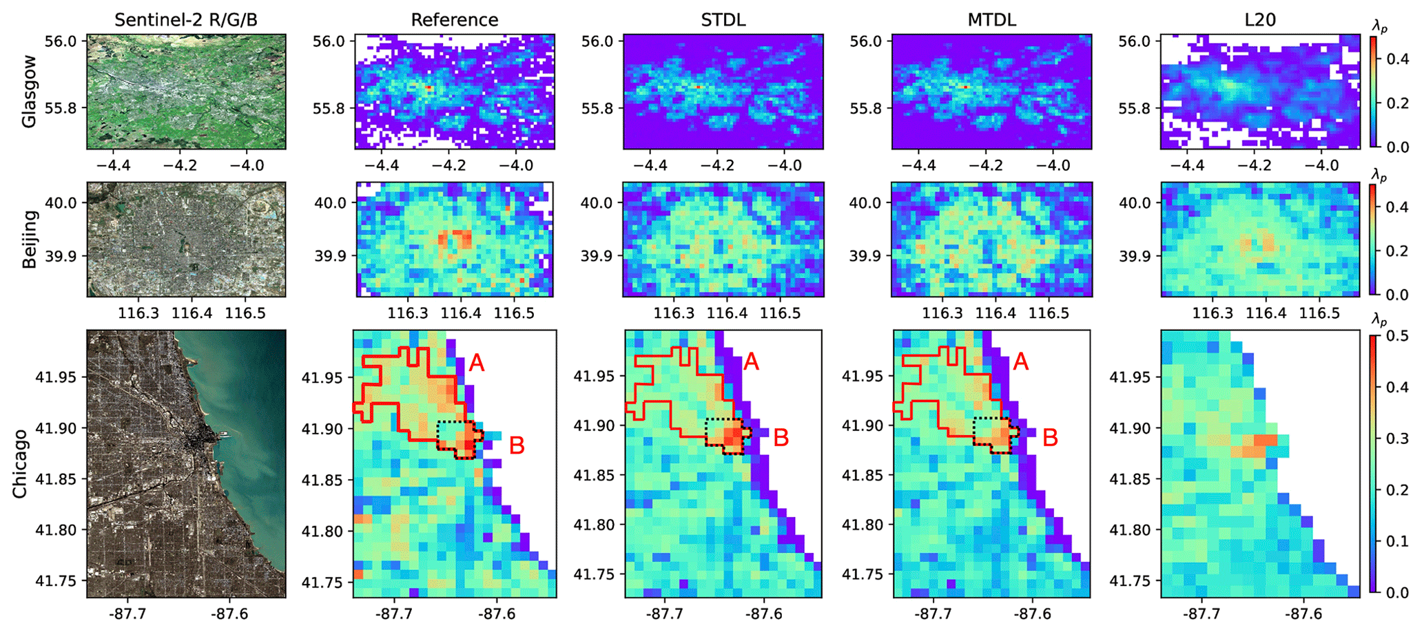
Figure 15Same as Fig. 14, but for building footprint. In Chicago, high-density built-up areas and surrounding areas of peak values are outlined by red lines and dotted black lines, respectively, where area A is determined based on the connected component analysis on the map of pixels with an average building footprint value higher than 0.3 and area B contains pixels with λp>0.5.
As mentioned before, publicly available reference data inevitably introduce noises and such noisy reference data pose a challenge to model performance evaluation, especially in terms of quantitative pixel-wise comparison (Burke et al., 2021). For example, after preliminary assessment of reference data quality in three cities, we found that for Chicago, although most building polygons exhibit satisfactory agreement with building footprints interpreted from aerial images, there are about 48 % of missing entries in the height field of building polygons, which may cause significant deviation between calculated reference and underlying truth. Thus, we only evaluate mapping results of Beijing and Chicago in a qualitative way.
For building height prediction, DL models can better capture peak values, especially for skyscrapers neighbouring Lake Michigan in Chicago (Fig. 14). However, overestimates are observed for a large area of Chicago and Beijing when compared with reference maps. While it agrees with the findings of overestimation in low-value domains based on a previous patch-level analysis (Fig. 6), it might also be caused by the bias in reference building height converted from the number of floors when compared with their actual values. Based on existing records of some iconic buildings and street view images given by the Baidu map (https://map.baidu.com/, last access: 1 November 2022) and Google Maps (https://www.google.com/maps/, last access: 1 November 2022), we find that deriving building height from the unit of floor numbers using a constant ratio of 3.0 may underestimate actual reference building height, especially for high risers. Take China Zun in Beijing for example, it has an actual height of 528 m but only 108 floors, which results in a 38.6 % underestimate if a height/floor ratio of 3.0 is used in the conversion. Thus, more advanced strategies would be desired if we aim to harmonize datasets from these two units for model development and evaluation.
Compared with building height, reference data of building footprint are expected to be more reliable based on the aforementioned data quality assessment. For building footprint prediction, all three models can give a relatively accurate estimation of the urban boundary and spatial distribution of building footprint. However, L20 tends to provide more blurred results such as the mapping for the south area of Beijing due to overestimation in building footprint. This over-smoothing phenomenon might be caused by the prediction strategy of RFR, where the final result was determined by a simple average of results from all trees (Hastie et al., 2009; Liu et al., 2021). Furthermore, all three models are likely to underestimate the peak values of high-density built-up areas, especially in Chicago. In the high-density built-up areas of Chicago (outlined by red lines in Fig. 15), STL and MTL models achieve comparable performance: the STL model exhibits better performance on the peak values but tends to overestimate the average built-up area in the corresponding surrounding region (outlined by dotted black lines in Fig. 15); while for the MTL model, it achieves a more satisfactory balance between the high and low values and gives slightly better predictions on these areas with respect to RMSE (0.061 for STL vs. 0.056 for MTL).
To investigate possible reasons why underestimation exists, we looked into the Sentinel-2's optical images of these areas: some buildings can hardly be identified precisely, even by human eyes, due to coarse resolution and misleading reflectance (not shown). Thus, besides Sentinel imagery, images with finer resolution or additional urban information such as multi-source datasets used in L20 may help to improve the building footprint prediction.
3.3.2 Quantitative evaluation in Glasgow
To perform quantitative evaluation under the challenge of noisy data, we focus our evaluation on urbanized areas with more reliable building morphological information. Thus, we implemented a post-processing algorithm for urban boundary extraction, the city clustering algorithm based on percolation theory (CCAP) (Cao et al., 2020), which utilizes the mapping results of building height and footprint to automatically determine an optimal threshold of the footprint value differentiating between urban and non-urban area (see Appendix B for details). In the following sections, we present Glasgow’s masked mappings and evaluation results after performing CCAP.
3D building structure mapping
The results of comparing our mappings and L20 with reference data are summarized in Table 4.
Table 4Building height and footprint prediction evaluated in Glasgow. Error metrics including RMSE, and CC are calculated using pixels from the intersection part of masked reference and predictions.
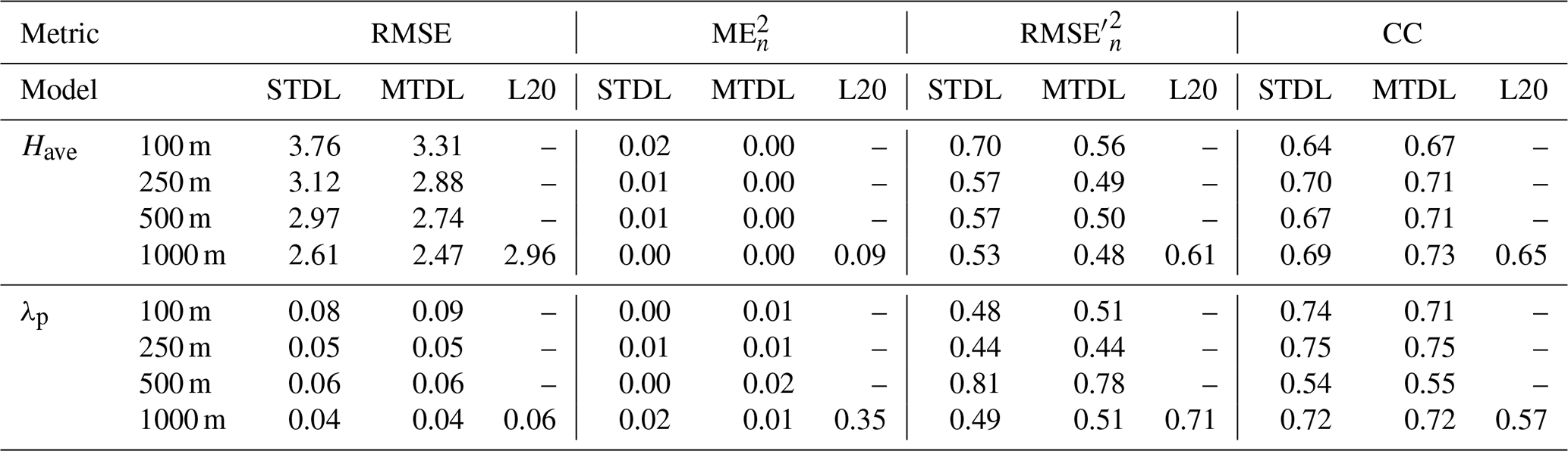
When compared with L20 that benefited from multi-source datasets, although our 1000 m mappings are merely based on Sentinel imagery, they still achieve 16.6 % and 33.3 % improvement on RMSE for building height and footprint estimation, respectively. For building height prediction, although L20 achieves a relatively close CC with DL models, it has much higher and than DL models and therefore suffers from overall performance degradation. A similar but much larger systematic bias can be observed for building footprint prediction when comparing L20 with the MTDL model. Thus, it can be concluded that systematic bias would greatly influence the performance of RFR at a relatively coarser resolution such as 1000 m, especially for building footprint mappings, which agrees with previous statistical results derived from the decomposition of 1−R2 (Sect. 3.2.3).
Moreover, we compare the performance with respect to STDL and MTDL models. For building height prediction, when compared with STDL models, MTDL models achieve better performance in all cases, especially for the case of 100 m where the MTDL model reduces the RMSE by 0.45 m. From the decomposition part of RMSE at the case of 100 m, this can mainly be attributed to the decrease of , which indicates that the MTDL model captures the variability of building height more correctly than the STDL model when target resolution becomes refined. This phenomenon seems contradictory to previous patch-level results and our intuitions that multi-task learning might hurt the performance as the size of input patches decreases because less information is available for correlating building height with footprint. Nevertheless, since multi-task learning necessitates a trade-off for a single model by joint optimization of two prediction tasks and further constrains the parameter space of desired models (Sener and Koltun, 2018), MTDL models can be expected to have better generalization ability and reduced risk of fitting noises. This might help us to understand why MTDL models can exhibit better performance of building height prediction in the spatial transferability testing at a refined scale such as 100 m. For building footprint prediction, STDL and MTDL models achieve almost the same performance in terms of both RMSE and its decomposed parts.
Since above error metrics assess model performance in an average sense, we further plotted the predicted spatial distribution of building height and footprint in Figs. 16 and 17, respectively, with medians of corresponding bias in different target domains. For both building height and footprint mappings, our models can clearly resolve central urban area and corresponding peak values. However, for all cases, urban area identified from predictions are larger than those derived from reference, especially for the 100 m case. It is mainly caused by the fact that a large number of external pixels lying outside the central area have small height values due to missing data so that they would always be identified as non-urban pixels during the process of CCAP. No significant difference can be found when we compare spatial distributions of Have and λp predicted by STDL and MTDL models. However, plots of medians of bias in Figs. 16 and 17 reveal that although STDL and MTDL models still exhibit relatively small performance gaps for all target domains of Have, they mainly differ in the domain where Have≥21 m, especially for cases of 100 and 1000 m. In that domain of the case of 100 m, the STDL model shows a much smaller absolute value of the median of bias. This phenomenon seems to disagree with previous results obtained by the comparison of RMSE. However, it should be noted that stratified bias analysis neglects sample frequency of target domains and therefore can lead to its disagreement with error metrics derived by averaging of overall samples.
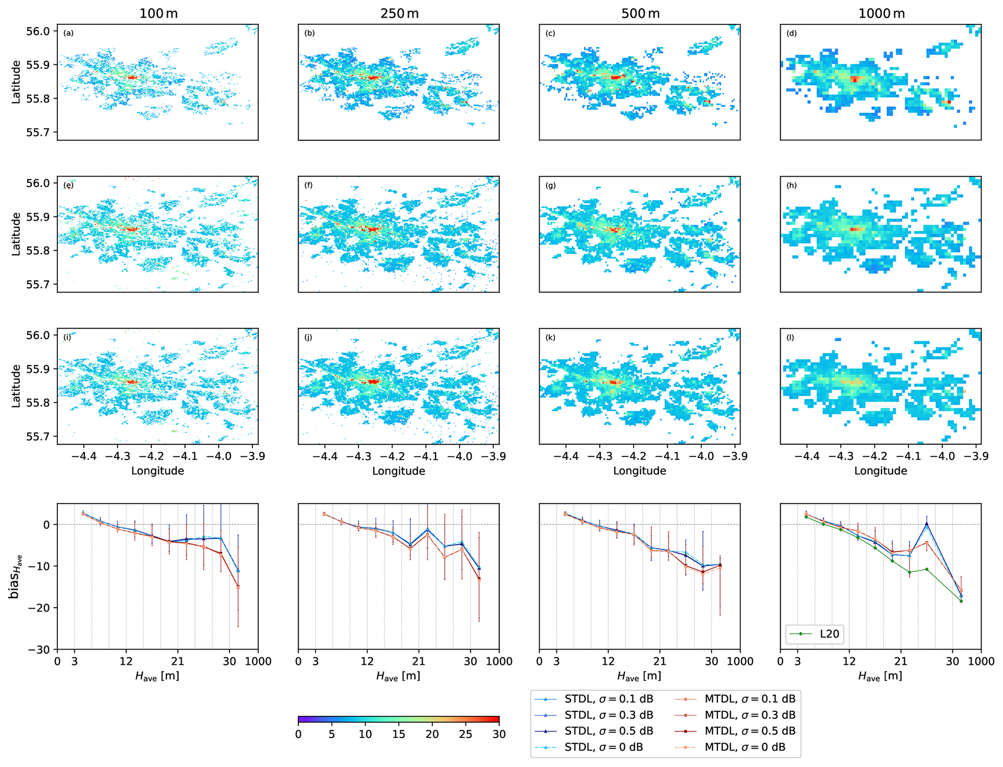
Figure 16Building height prediction in Glasgow with corresponding stratified bias distribution. (a–d) Reference building height maps. (e–h) Building height maps predicted by STDL models. (i–l) Building height maps predicted by MTDL models. The bias is equal to prediction minus reference. σ is the standard deviation of Gaussian noises injected into the Sentinel-1's VV and VH bands. σ=0 dB stands for the results using original Sentinel's images with no noise injected. Uncertainty in each target domain is expressed as a vertical line whose upper, lower bounds and middle points represent the quartiles of bias distribution. Target domains of building height are divided by 3, 6, 9, 12, 15, 18, 21, 24, 27 and 30 m. Domains without valid samples are omitted.
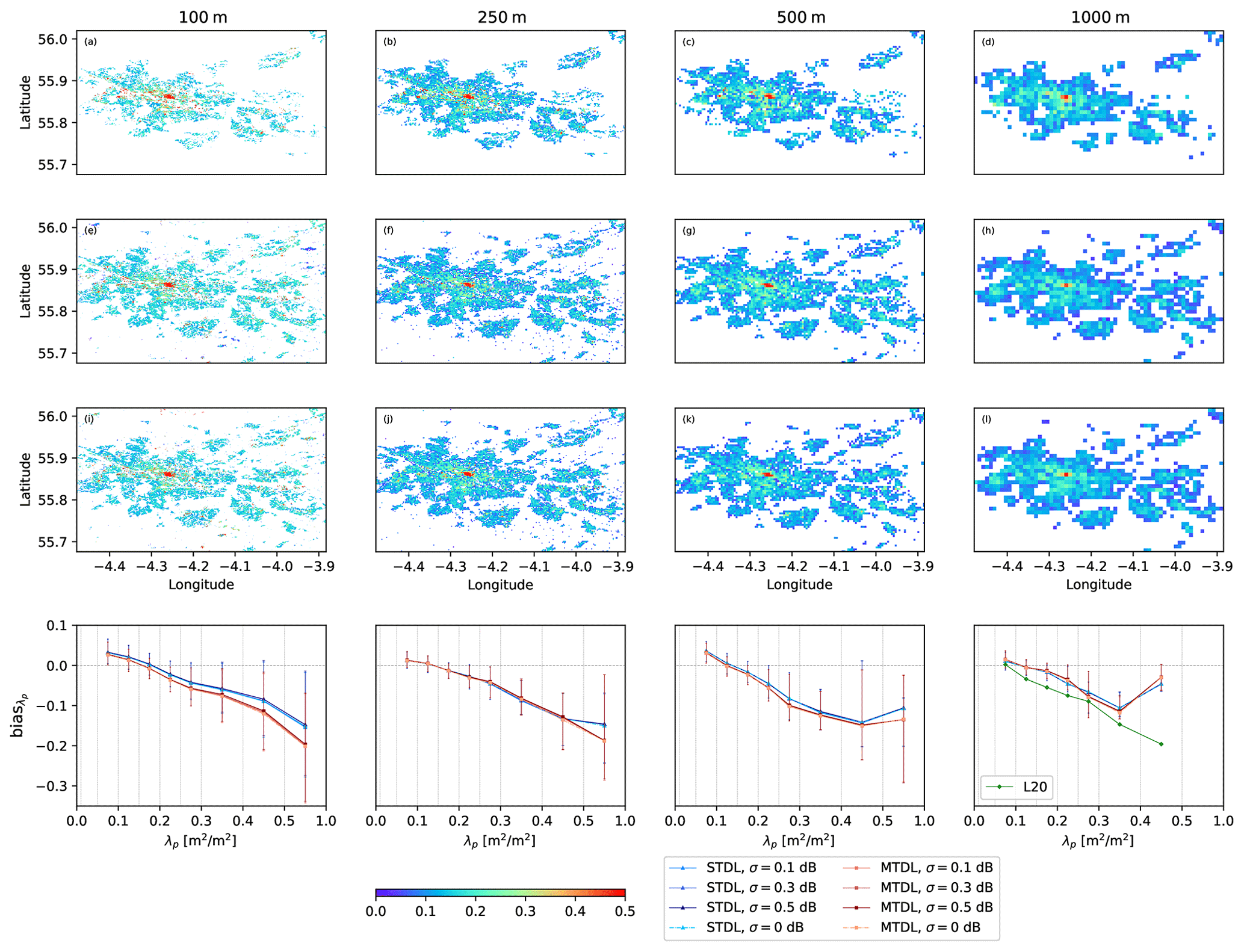
Figure 17Same as Fig. 16, but for building footprint and corresponding target domains are divided by 0.001, 0.01, 0.05, 0.1, 0.15, 0.20, 0.25, 0.3, 0.4 and 0.5.
Moreover, stratified bias analysis also gives new insights into the comparison between L20 and proposed DL models. For building height prediction, although L20 achieves a slightly smaller absolute value of the median of bias in the domain where Have<10 m, the performance gap between L20 and proposed DL models is reversed and then enlarged up to 10 m in the domain where . A similar performance gap up to 0.15 can also be observed for building footprint prediction ranging from 0.4 to 0.5. Thus, it can be concluded that multi-source information still fails to effectively compensate for the weakness of ML models in predicting high risers and high-density built-up areas and therefore, promoting advances in model architecture can be expected to bring more benefits.
Uncertainty analysis of input Sentinel-1's band
To further investigate potential effects caused by radiometric performance degradation of Sentinel-1's images on 3D building information mapping, we performed an uncertainty analysis on prediction results by injecting random noises to the input VV and VH bands. Specifically, according to absolute radiometric accuracy for the IW mode reported in the official Sentinel-1 annual performance report for 2020, we designed three levels of zero-mean Gaussian noises with standard deviation σ=0.1, 0.3, 0.5 dB. Moreover, for each level of noises and target resolution, we performed 50 random simulations by adding independent noises to original VV and VH bands. Figures 16 and 17 show quartiles of bias distribution over different target domains derived from random simulations. By comparing quartiles of stratified bias under different levels of radiometric noises, no significant variation can be observed when the noise level increases from 0.1 to 0.5 dB, which demonstrates the robustness of DL models with respect to internal noises with σ<0.5 dB. Furthermore, when comparing STDL with MTDL models, the approximate invariance of stratified bias distributions can lead to similar conclusions drawn from original uncorrupted images with respect to the median of bias. However, for building height prediction, relatively more minor uncertainty of bias measured by IQR is presented by MTDL models in the high-value domain, such as Have≥24 m in the case of 100 m. It can be naturally attributed to the aforementioned regularization effect merited from multi-task learning. Thus, MTDL models can be promising in reducing the uncertainty of peak value prediction as well as increasing overall accuracy (cf. Table 4) for the refined building height mapping.
In this work, we develop a MTDL Python package, SHAFTS, for the simultaneous extraction of both building height and footprint from Sentinel imagery in urban areas. Comparison with conventional ML and STDL models in 46 cities worldwide demonstrates the following:
-
DL models – both STDL and MTDL – avoid tedious feature engineering by automatic data representation and outperform their ML counterparts in building height and footprint prediction for 38 cities by 0.27–0.63 and 0.11–0.49 measured by R2, respectively. Particularly, DL models effectively mitigate the saturation effect of ML models in high-value domains: for building height prediction, RMSE is reduced by 31 m when target height is higher than 40 m; for building footprint prediction, RMSE is reduced by 0.1 when target footprint is larger than 0.25.
-
Within the DL family, MTDL models achieve higher efficiency than STDL models by halving the number of required parameters and exhibit better generalization ability (e.g. in Glasgow with an improvement of 0.45 m in building height prediction measured by RMSE as well as reduced uncertainty of bias for the prediction of building height higher than 24 m for the case of 100 m).
Furthermore, we establish a diagnostic evaluation framework based on a two-step decomposition analysis, which can better interpret the performance variation across different models and target resolutions. Using this framework, we find that DL models outperform ML models in both systematic bias control and variability error reduction. In addition, relatively large systematic bias may significantly deteriorate the performance of ML models at coarse resolutions (e.g. >1000 m) and high-value domains.
Being promising for 3D building mapping in a large scale, the MTDL models in SHAFTS have several limitations that need to be appreciated here. Overestimation on building height and underestimation on building footprint of the developed MTDL model is observed in some densely built-up areas, which could be caused by the limited spatial resolution of Sentinel imagery and caveats in the designed models. Also, the inherent noises in reference data may influence the accuracy in assessing model performance. Therefore, robustness of the MTDL model will be tested in more cities in our forthcoming work. Moreover, the fusion of multi-source input data and more advanced ensemble strategies between ML and DL models will be conducted to address these issues and improve the prediction of urban morphological features.
A1 Feature extraction and preprocessing
To prepare the inputs for ML models, following (Geiß et al., 2020), 396 features are manually designed and extracted from sample patches in three aspects (see Table A1 for summary):
-
single-band statistic – the mean, standard deviation, maximum, minimum, 25th percentile, 50th percentile and 75th percentile of SRTM DEM, Sentinel-1's VV, VH bands and Sentinel-2's red, green, blue and NIR bands;
-
multi-spectral information – six normalized difference spectral indices and a brightness measure (Zhang et al., 2017);
-
morphological and texture quantities – differential morphological profiles (DMP) and grey-level co-occurrence matrix (GLCM) calculated using a square-shaped structuring element with six ascending sizes . Based on DMP and GLCM, several morphological and texture features were derived using different aggregation functions.
Table A1Features extracted from Sentinel-1 and Sentinel-2 imagery as the inputs of ML models. More details on feature description and calculation methods can be found in Geiß et al. (2020); Haralick et al. (1973); and Pesaresi and Benediktsson (2001).
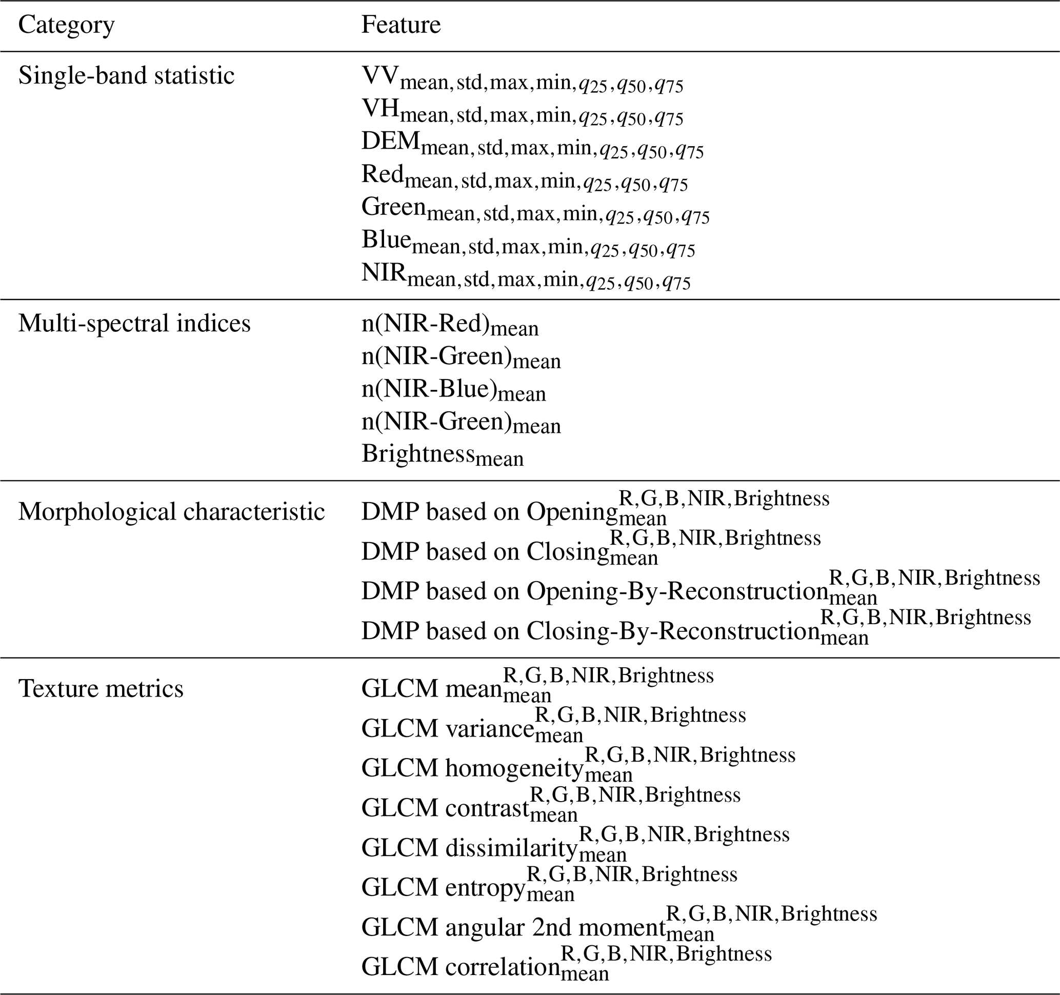
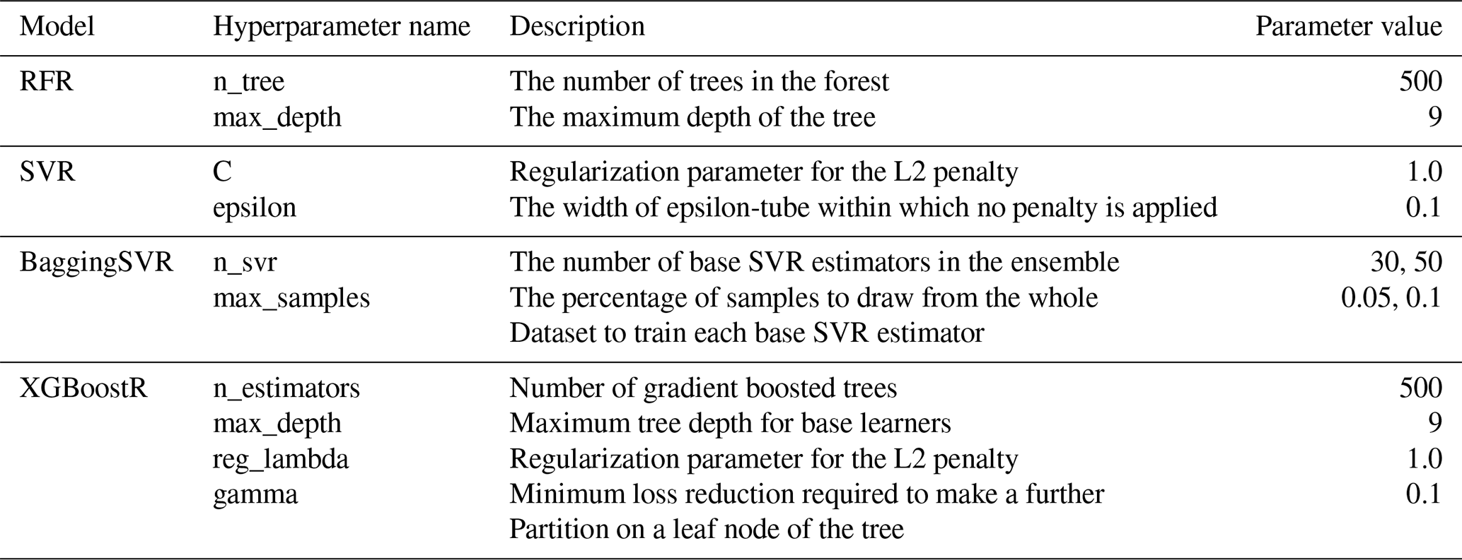
Table A2Hyperparameters optimization for ML models. For BaggingSVR, we choose n_svr=40 and max_samples=0.05 for the case of 100 m, n_svr=50 and max_samples=0.1 for the case of 250 m.
To reduce information redundancy and irrelevant noises in high-dimensional data, we preprocess features in the following steps:
-
Filtering – raw features with variance lower than 1e−6 are removed from the input feature set.
-
Normalization – remaining features are standardized by removing individual means and scaling to unit variance.
-
Transformation – principal component analysis is performed on normalized features to project them onto a lower dimensional space with a reduction ratio of 50 %.
A2 ML models
This work selects RFR, XGBoostR, SVR and its bagging version (BaggingSVR) as baseline models for comparison with DL models. It should be emphasized that while accuracy is our major concern for model selection, scalability is another crucial factor if the model would be applied to real-world situations for massive data mining. Compared with RFR and XGBoostR, most existing implementations of SVR with nonlinear kernels exhibits poorer scalability since it involves the solution of a quadratic optimization problem, which often requires well-designed decomposition algorithms (Joachims, 1998). Thus, when predicting about the dataset with the resolution of 100 and 250 m, the original SVR is replaced with a bagging regressor (Breiman, 1996), i.e. BaggingSVR, which trains SVR on random subsets of the original dataset as base estimators and then makes the final prediction with the aggregation of individual results. For notational simplicity, we denote both of them as SVR.
To guarantee the reliability of our research, we use widely used open-source Python packages for the implementation of ML models: scikit-learn (Varoquaux et al., 2015) for preprocessing pipelines, RFR, SVR and XGBoost (Chen and Guestrin, 2016) for XGBoostR (see key hyperparameter values in Table A2).
The procedure of CCAP can be summarized into the following steps:
-
Construct a potential building footprint threshold set with uniform spacings:
-
Determine an optimal footprint threshold based on percolation theory (Cao et al., 2020):
where Entropy(⋅) is the Shannon's entropy of the size distribution of the urban cluster system. Here a pixel is identified as an urban pixel if its building height and footprint value (λp,Have) satisfies and urban clusters are extracted by the Connected Component Analysis algorithm provided in the
OpenCVpackage (https://github.com/opencv/opencv, last access: 1 November 2022). -
Determine the threshold for final masking. Since different optimal thresholds can be calculated from the mapping results of various models (e.g. STDL and MTDL models), final masking can be derived by some simple fusion rules. In this work, we consider a pixel as an urban pixel if it is identified so in any mapping result.
The snapshot of source codes and reference datasets has been archived as a zipped file on Zenodo (https://doi.org/10.5281/zenodo.6587510, Li and Sun, 2022) to guarantee the reproducibility of our research. The up-to-date version of SHAFTS is available at: https://github.com/LllC-mmd/3DBuildingInfoMap (last access: 27 January 2023). SHAFTS is also accessible via the Python pip package manager.
The supplement related to this article is available online at: https://doi.org/10.5194/gmd-16-751-2023-supplement.
RL led the development of SHAFTS. RL and TS performed the formal analysis. TS, GN and FT contributed to the computing resources and supervision. RL wrote the original draft and all authors contributed to reviewing and editing of the paper.
The contact author has declared that none of the authors has any competing interests.
Publisher’s note: Copernicus Publications remains neutral with regard to jurisdictional claims in published maps and institutional affiliations.
This work was supported by the National Key Research and Development Program of China (2018YFA0606002), the Fund Program of State Key Laboratory of Hydroscience and Engineering (61010101221), Open Research Fund Program of State Key Laboratory of Hydroscience and Engineering (sklhse-2020-A06), NERC Independent Research Fellowship (NE/P018637/2).
This research has been supported by the National Key Research and Development Programme of China (grant no. 2018YFA0606002), the Fund Program of State Key Laboratory of Hydroscience and Engineering (61010101221), Open Research Fund Program of State Key Laboratory of Hydroscience and Engineering (sklhse-2020A06) and NERC Independent Research Fellowship (NE/P018637/2).
This paper was edited by Richard Mills and reviewed by two anonymous referees.
Bengio, Y., Courville, A., and Vincent, P.: Representation Learning: A Review and New Perspectives, IEEE T. Pattern Anal., 35, 1798–1828, https://doi.org/10.1109/tpami.2013.50, 2013. a, b
Breiman, L.: Bagging predictors, Mach. Learn., 24, 123–140, 1996. a
Brunner, D., Lemoine, G., Bruzzone, L., and Greidanus, H.: Building Height Retrieval From VHR SAR Imagery Based on an Iterative Simulation and Matching Technique, IEEE T. Geosci. Remote, 48, 1487–1504, https://doi.org/10.1109/tgrs.2009.2031910, 2010. a
Bruwier, M., Maravat, C., Mustafa, A., Teller, J., Pirotton, M., Erpicum, S., Archambeau, P., and Dewals, B.: Influence of urban forms on surface flow in urban pluvial flooding, J. Hydrol., 582, 124493, https://doi.org/10.1016/j.jhydrol.2019.124493, 2020. a
Burke, M., Driscoll, A., Lobell, D. B., and Ermon, S.: Using satellite imagery to understand and promote sustainable development, Science, 371, eabe8626, https://doi.org/10.1126/science.abe8628, 2021. a, b
Cao, W., Dong, L., Wu, L., and Liu, Y.: Quantifying urban areas with multi-source data based on percolation theory, Remote Sens. Environ., 241, 111730, https://doi.org/10.1016/j.rse.2020.111730, 2020. a, b
Cao, Y. and Huang, X.: A deep learning method for building height estimation using high-resolution multi-view imagery over urban areas: A case study of 42 Chinese cities, Remote Sens. Environ., 264, 112590, https://doi.org/10.1016/j.rse.2021.112590, 2021. a, b, c, d, e
Carrera-Hernández, J.: Not all DEMs are equal: An evaluation of six globally available 30 m resolution DEMs with geodetic benchmarks and LiDAR in Mexico, Remote Sens. Environ., 261, 112474, https://doi.org/10.1016/j.rse.2021.112474, 2021. a
Caruana, R.: Multitask learning, Mach. Learn., 28, 41–75, 1997. a
Chen, T. and Guestrin, C.: XGBoost, in: Proceedings of the 22nd ACM SIGKDD International Conference on Knowledge Discovery and Data Mining, KDD '16, ACM, New York, NY, USA, 13–17 August 2016, 785–794, https://doi.org/10.1145/2939672.2939785, 2016. a, b
Chen, Z., Badrinarayanan, V., Lee, C.-Y., and Rabinovich, A.: Gradnorm: Gradient normalization for adaptive loss balancing in deep multitask networks, in: International Conference on Machine Learning, Stockholm, Sweden, 10–15 July 2018, arXiv [preprint], https://doi.org/10.48550/arXiv.1711.02257, 794–803, PMLR, 2018. a
Cipolla, R., Gal, Y., and Kendall, A.: Multi-task Learning Using Uncertainty to Weigh Losses for Scene Geometry and Semantics, in: 2018 IEEE Conference on Computer Vision and Pattern Recognition, Salt Lake City, USA, 18–23 June 2018, 7482–7491, IEEE, https://doi.org/10.1109/cvpr.2018.00781, 2018. a, b
Drusch, M., Del Bello, U., Carlier, S., Colin, O., Fernandez, V., Gascon, F., Hoersch, B., Isola, C., Laberinti, P., Martimort, P., Meygret, A., Spoto, F., Sy, O., Marchese, F., and Bargellini, P.: Sentinel-2: Esa's Optical High-Resolution Mission for GMES Operational Services, Remote Sens. Environ., 120, 25–36, https://doi.org/10.1016/j.rse.2011.11.026, 2012. a
Eigen, D. and Fergus, R.: Predicting Depth, Surface Normals and Semantic Labels with a Common Multi-scale Convolutional Architecture, in: 2015 IEEE International Conference on Computer Vision, Santiago, Chile, 7–13 December 2015, 2650–2658, IEEE, https://doi.org/10.1109/iccv.2015.304, 2015. a
Esch, T., Brzoska, E., Dech, S., Leutner, B., Palacios-Lopez, D., Metz-Marconcini, A., Marconcini, M., Roth, A., and Zeidler, J.: World Settlement Footprint 3D – A first three-dimensional survey of the global building stock, Remote Sens. Environ., 270, 112877, https://doi.org/10.1016/j.rse.2021.112877, 2022. a, b
Frantz, D., Schug, F., Okujeni, A., Navacchi, C., Wagner, W., van der Linden, S., and Hostert, P.: National-scale mapping of building height using Sentinel-1 and Sentinel-2 time series, Remote Sens. Environ., 252, 112128, https://doi.org/10.1016/j.rse.2020.112128, 2021. a, b, c, d, e, f, g, h, i, j, k, l
Frolking, S., Milliman, T., Seto, K. C., and Friedl, M. A.: A global fingerprint of macro-scale changes in urban structure from 1999 to 2009, Environ. Res. Lett., 8, 024004, https://doi.org/10.1088/1748-9326/8/2/024004, 2013. a
Geiß, C., Leichtle, T., Wurm, M., Pelizari, P. A., Standfuß, I., Zhu, X. X., So, E., Siedentop, S., Esch, T., and Taubenböck, H.: Large-Area Characterization of Urban Morphology–Mapping of Built-Up Height and Density Using TanDEM-X and Sentinel-2 Data, IEEE J. Sel. Top. Appl., 12, 2912–2927, https://doi.org/10.1109/JSTARS.2019.2917755, 2019. a
Geiß, C., Schrade, H., Aravena Pelizari, P., and Taubenböck, H.: Multistrategy ensemble regression for mapping of built-up density and height with Sentinel-2 data, ISPRS J. Photogramm., 170, 57–71, https://doi.org/10.1016/j.isprsjprs.2020.10.004, 2020. a, b, c, d, e, f, g
Gorelick, N., Hancher, M., Dixon, M., Ilyushchenko, S., Thau, D., and Moore, R.: Google Earth Engine: Planetary-scale geospatial analysis for everyone, Remote Sens. Environ., 202, 18–27, https://doi.org/10.1016/j.rse.2017.06.031, 2017. a
Grimm, N. B., Faeth, S. H., Golubiewski, N. E., Redman, C. L., Wu, J., Bai, X., and Briggs, J. M.: Global Change and the Ecology of Cities, Science, 319, 756–760, https://doi.org/10.1126/science.1150195, 2008. a
Guo, H., Shi, Q., Du, B., Zhang, L., Wang, D., and Ding, H.: Scene-Driven Multitask Parallel Attention Network for Building Extraction in High-Resolution Remote Sensing Images, IEEE T. Geosci. Remote, 59, 4287–4306, https://doi.org/10.1109/tgrs.2020.3014312, 2021. a, b
Gupta, H. V., Kling, H., Yilmaz, K. K., and Martinez, G. F.: Decomposition of the mean squared error and NSE performance criteria: Implications for improving hydrological modelling, J. Hydrol., 377, 80–91, https://doi.org/10.1016/j.jhydrol.2009.08.003, 2009. a, b
Haralick, R. M., Shanmugam, K., and Dinstein, I.: Textural Features for Image Classification, IEEE T. Syst. Man Cyb., SMC-3, 610–621, https://doi.org/10.1109/tsmc.1973.4309314, 1973. a
Hastie, T., Tibshirani, R., and Friedman, J.: The Elements of Statistical Learning, Springer New York, https://doi.org/10.1007/978-0-387-84858-7, 2009. a, b, c
He, K., Zhang, X., Ren, S., and Sun, J.: Deep Residual Learning for Image Recognition, in: 2016 IEEE Conference on Computer Vision and Pattern Recognition, Las Vegas, USA, 27–30 June 2016, 770–778, IEEE, https://doi.org/10.1109/cvpr.2016.90, 2016. a, b
Hu, J., Shen, L., and Sun, G.: Squeeze-and-Excitation Networks, in: 2018 IEEE Conference on Computer Vision and Pattern Recognition, Salt Lake City, USA, 18–23 June 2018, 7132–7141, IEEE, https://doi.org/10.1109/cvpr.2018.00745, 2018. a, b, c
Huber, P. J.: Robust Estimation of a Location Parameter, Ann. Math. Stat., 35, 73–101, https://doi.org/10.1214/aoms/1177703732, 1964. a
Ji, C. and Tang, H.: Number of Building Stories Estimation from Monocular Satellite Image Using a Modified Mask R-CNN, Remote Sensing, 12, 3833, https://doi.org/10.3390/rs12223833, 2020. a
Joachims, T.: Making large-scale SVM learning practical, Technical report, http://hdl.handle.net/10419/77178 (last access date: 20 January 2023), 1998. a
Koppel, K., Zalite, K., Voormansik, K., and Jagdhuber, T.: Sensitivity of Sentinel-1 backscatter to characteristics of buildings, Int. J. Remote Sens., 38, 6298–6318, https://doi.org/10.1080/01431161.2017.1353160, 2017. a, b
Lagacherie, P., Rabotin, M., Colin, F., Moussa, R., and Voltz, M.: Geo-MHYDAS: A landscape discretization tool for distributed hydrological modeling of cultivated areas, Comput. Geosci., 36, 1021–1032, https://doi.org/10.1016/j.cageo.2009.12.005, 2010. a
LeCun, Y., Bengio, Y., and Hinton, G.: Deep learning, Nature, 521, 436–444, https://doi.org/10.1038/nature14539, 2015. a, b
Li, M., Koks, E., Taubenböck, H., and van Vliet, J.: Continental-scale mapping and analysis of 3D building structure, Remote Sens. Environ., 245, 111859, https://doi.org/10.1016/j.rse.2020.111859, 2020. a, b, c, d, e, f, g, h, i, j, k
Li, R. and Sun, T.: Reference Datasets for: SHAFTS (v2022.3): a deep-learning-based Python package for Simultaneous extraction of building Height And FootprinT from Sentinel Imagery, Zenodo [data set], https://doi.org/10.5281/zenodo.6587510, 2022. a
Liebel, L., Bittner, K., and Körner, M.: A generalized multi-task learning approach to stereo DSM filtering in urban areas, ISPRS J. Photogramm., 166, 213–227, https://doi.org/10.1016/j.isprsjprs.2020.03.005, 2020. a
Liu, Y., Bates, P. D., Neal, J. C., and Yamazaki, D.: Bare-Earth DEM Generation in Urban Areas for Flood Inundation Simulation Using Global Digital Elevation Models, Water Resour. Res., 57, e2020WR028516, https://doi.org/10.1029/2020wr028516, 2021. a
Loew, A. and Mauser, W.: Generation of geometrically and radiometrically terrain corrected SAR image products, Remote Sens. Environ., 106, 337–349, https://doi.org/10.1016/j.rse.2006.09.002, 2007. a
Loshchilov, I. and Hutter, F.: SGDR: Stochastic Gradient Descent with Warm Restarts, in: 5th International Conference on Learning Representations, OpenReview.net, Toulon, France, 24–26 April 2017, arXiv [preprint], https://doi.org/10.48550/arXiv.1608.03983, 2017. a
Masson, V., Heldens, W., Bocher, E., Bonhomme, M., Bucher, B., Burmeister, C., de Munck, C., Esch, T., Hidalgo, J., Kanani-Sühring, F., Kwok, Y.-T., Lemonsu, A., Lévy, J.-P., Maronga, B., Pavlik, D., Petit, G., See, L., Schoetter, R., Tornay, N., Votsis, A., and Zeidler, J.: City-descriptive input data for urban climate models: Model requirements, data sources and challenges, Urban Clim., 31, 100536, https://doi.org/10.1016/j.uclim.2019.100536, 2020a. a
Masson, V., Lemonsu, A., Hidalgo, J., and Voogt, J.: Urban Climates and Climate Change, Annu. Rev. Env. Resour., 45, 411–444, https://doi.org/10.1146/annurev-environ-012320-083623, 2020b. a
Mirzaei, P. A. and Haghighat, F.: Approaches to study Urban Heat Island – Abilities and limitations, Build. Environ., 45, 2192–2201, https://doi.org/10.1016/j.buildenv.2010.04.001, 2010. a
Moreira, A., Prats-Iraola, P., Younis, M., Krieger, G., Hajnsek, I., and Papathanassiou, K. P.: A tutorial on synthetic aperture radar, IEEE Geoscience and Remote Sensing Magazine, 1, 6–43, https://doi.org/10.1109/MGRS.2013.2248301, 2013. a
Mottaghi, R., Chen, X., Liu, X., Cho, N.-G., Lee, S.-W., Fidler, S., Urtasun, R., and Yuille, A.: The Role of Context for Object Detection and Semantic Segmentation in the Wild, in: 2014 IEEE Conference on Computer Vision and Pattern Recognition, Columbus, USA, 23–28 June 2014, 891–898, https://doi.org/10.1109/CVPR.2014.119, 2014. a
Nosek, B. A., Alter, G., Banks, G. C., Borsboom, D., Bowman, S. D., Breckler, S. J., Buck, S., Chambers, C. D., Chin, G., Christensen, G., Contestabile, M., Dafoe, A., Eich, E., Freese, J., Glennerster, R., Goroff, D., Green, D. P., Hesse, B., Humphreys, M., Ishiyama, J., Karlan, D., Kraut, A., Lupia, A., Mabry, P., Madon, T., Malhotra, N., Mayo-Wilson, E., McNutt, M., Miguel, E., Paluck, E. L., Simonsohn, U., Soderberg, C., Spellman, B. A., Turitto, J., VandenBos, G., Vazire, S., Wagenmakers, E. J., Wilson, R., and Yarkoni, T.: Promoting an open research culture, Science, 348, 1422–1425, https://doi.org/10.1126/science.aab2374, 2015. a
Pesaresi, M. and Benediktsson, J.: A new approach for the morphological segmentation of high-resolution satellite imagery, IEEE T. Geosci. Remote, 39, 309–320, https://doi.org/10.1109/36.905239, 2001. a
Piantanida, R., Hajduch, G., and Poullaouec, J.: Sentinel-1 Level 1 Detailed Algorithm Definition, ESA, techreport SEN-TN-52-7445, https://sentinels.copernicus.eu/web/sentinel/user-guides/sentinel-1-sar/document-library/-/asset_publisher/1dO7RF5fJMbd/content/id/2477988 (last access: 1 November 2022), 2021. a
Qin, Z., Zhang, P., Wu, F., and Li, X.: FcaNet: Frequency Channel Attention Networks, Montreal, Canada, 10–17 October 2021. 783–792, https://doi.org/10.1109/ICCV48922.2021.00082, 2021. a
Ruder, S.: An Overview of Multi-Task Learning in Deep Neural Networks, arXiv [preprint], https://doi.org/10.48550/arXiv.1706.05098, 15 June 2017. a
Salvadore, E., Bronders, J., and Batelaan, O.: Hydrological modelling of urbanized catchments: A review and future directions, J. Hydrol., 529, 62–81, https://doi.org/10.1016/j.jhydrol.2015.06.028, 2015. a
Sampson, C. C., Smith, A. M., Bates, P. D., Neal, J. C., Alfieri, L., and Freer, J. E.: A high-resolution global flood hazard model, Water Resour. Res., 51, 7358–7381, https://doi.org/10.1002/2015wr016954, 2015. a
Schaefli, B. and Gupta, H. V.: Do Nash values have value?, Hydrol. Process., 21, 2075–2080, https://doi.org/10.1002/hyp.6825, 2007. a
Sener, O. and Koltun, V.: Multi-task learning as multi-objective optimization, in: Proceedings of the 32nd International Conference on Neural Information Processing Systems, Montreal, Canada, 3–8 December 2018, arXiv [preprint], https://doi.org/10.48550/arXiv.1810.04650, 525–536, 2018. a, b
Shi, Y., Li, Q., and Zhu, X. X.: Building segmentation through a gated graph convolutional neural network with deep structured feature embedding, ISPRS J. Photogramm., 159, 184–197, https://doi.org/10.1016/j.isprsjprs.2019.11.004, 2020. a, b
Shorten, C. and Khoshgoftaar, T. M.: A survey on Image Data Augmentation for Deep Learning, Journal of Big Data, 6, 1–48, https://doi.org/10.1186/s40537-019-0197-0, 2019. a
Simonyan, K. and Zisserman, A.: Very Deep Convolutional Networks for Large-Scale Image Recognition, in: 3rd International Conference on Learning Representations, edited by: Bengio, Y. and LeCun, Y., San Diego, USA, 7–9 May 2015, arXiv [preprint], https://doi.org/10.48550/arXiv.1409.1556, 2015. a
Soergel, B., Kriegler, E., Weindl, I., Rauner, S., Dirnaichner, A., Ruhe, C., Hofmann, M., Bauer, N., Bertram, C., Bodirsky, B. L., Leimbach, M., Leininger, J., Levesque, A., Luderer, G., Pehl, M., Wingens, C., Baumstark, L., Beier, F., Dietrich, J. P., Humpenöder, F., von Jeetze, P., Klein, D., Koch, J., Pietzcker, R., Strefler, J., Lotze-Campen, H., and Popp, A.: A sustainable development pathway for climate action within the UN 2030 Agenda, Nat. Clim. Change, 11, 656–664, https://doi.org/10.1038/s41558-021-01098-3, 2021. a
Stilla, U., Soergel, U., and Thoennessen, U.: Potential and limits of InSAR data for building reconstruction in built-up areas, ISPRS J. Photogramm., 58, 113–123, https://doi.org/10.1016/s0924-2716(03)00021-2, 2003. a
Sun, Y., Mou, L., Wang, Y., Montazeri, S., and Zhu, X. X.: Large-scale building height retrieval from single SAR imagery based on bounding box regression networks, ISPRS J. Photogramm., 184, 79–95, https://doi.org/10.1016/j.isprsjprs.2021.11.024, 2022. a
Szegedy, C., Liu, W., Jia, Y., Sermanet, P., Reed, S. E., Anguelov, D., Erhan, D., Vanhoucke, V., and Rabinovich, A.: Going deeper with convolutions, in: 2015 IEEE Conference on Computer Vision and Pattern Recognition, Boston, USA, 7–12 June 2015, 1–9, IEEE, https://doi.org/10.1109/CVPR.2015.7298594, 2015. a
Taylor, K. E.: Summarizing multiple aspects of model performance in a single diagram, J. Geophys. Res.-Atmos., 106, 7183–7192, https://doi.org/10.1029/2000jd900719, 2001. a, b, c, d
Torres, R., Snoeij, P., Geudtner, D., Bibby, D., Davidson, M., Attema, E., Potin, P., Rommen, B., Floury, N., Brown, M., Traver, I. N., Deghaye, P., Duesmann, B., Rosich, B., Miranda, N., Bruno, C., L'Abbate, M., Croci, R., Pietropaolo, A., Huchler, M., and Rostan, F.: GMES Sentinel-1 mission, Remote Sens. Environ., 120, 9–24, https://doi.org/10.1016/j.rse.2011.05.028, 2012. a
van der Maaten, L. and Hinton, G.: Visualizing non-metric similarities in multiple maps, Mach. Learn., 87, 33–55, https://doi.org/10.1007/s10994-011-5273-4, 2011. a
Varoquaux, G., Buitinck, L., Louppe, G., Grisel, O., Pedregosa, F., and Mueller, A.: Scikit-learn, GetMobile: Mobile Computing and Communications, 19, 29–33, https://doi.org/10.1145/2786984.2786995, 2015. a
Yu, B., Liu, H., Wu, J., Hu, Y., and Zhang, L.: Automated derivation of urban building density information using airborne LiDAR data and object-based method, Landscape Urban Plan., 98, 210–219, https://doi.org/10.1016/j.landurbplan.2010.08.004, 2010. a
Yu, Z., Hu, L., Sun, T., Albertson, J., and Li, Q.: Impact of heat storage on remote-sensing based quantification of anthropogenic heat in urban environments, Remote Sens. Environ., 262, 112520, https://doi.org/10.1016/j.rse.2021.112520, 2021. a
Zhang, T., Huang, X., Wen, D., and Li, J.: Urban Building Density Estimation From High-Resolution Imagery Using Multiple Features and Support Vector Regression, IEEE J. Sel. Top. Appl., 10, 3265–3280, https://doi.org/10.1109/jstars.2017.2669217, 2017. a
Zheng, Z., Zhou, W., Wang, J., Hu, X., and Qian, Y.: Sixty-Year Changes in Residential Landscapes in Beijing: A Perspective from Both the Horizontal (2D) and Vertical (3D) Dimensions, Remote Sensing, 9, 992, https://doi.org/10.3390/rs9100992, 2017. a
Zhong, Y., Su, Y., Wu, S., Zheng, Z., Zhao, J., Ma, A., Zhu, Q., Ye, R., Li, X., Pellikka, P., and Zhang, L.: Open-source data-driven urban land-use mapping integrating point-line-polygon semantic objects: A case study of Chinese cities, Remote Sens. Environ., 247, 111838, https://doi.org/10.1016/j.rse.2020.111838, 2020. a
Zhu, X., Cheng, D., Zhang, Z., Lin, S., and Dai, J.: An Empirical Study of Spatial Attention Mechanisms in Deep Networks, in: 2019 IEEE International Conference on Computer Vision, Seoul, Korea, 27 October–2 November 2019, 6688–6697, IEEE, https://doi.org/10.1109/iccv.2019.00679, 2019a. a
Zhu, X. X., Tuia, D., Mou, L., Xia, G.-S., Zhang, L., Xu, F., and Fraundorfer, F.: Deep Learning in Remote Sensing: A Comprehensive Review and List of Resources, IEEE Geoscience and Remote Sensing Magazine, 5, 8–36, https://doi.org/10.1109/mgrs.2017.2762307, 2017. a
Zhu, X. X., Qiu, C., Hu, J., Shi, Y., Wang, Y., Schmitt, M., and Taubenböck, H.: The urban morphology on our planet – Global perspectives from space, Remote Sens. Environ., 269, 112794, https://doi.org/10.1016/j.rse.2021.112794, 2022. a
Zhu, Z., Zhou, Y., Seto, K. C., Stokes, E. C., Deng, C., Pickett, S. T., and Taubenböck, H.: Understanding an urbanizing planet: Strategic directions for remote sensing, Remote Sens. Environ., 228, 164–182, https://doi.org/10.1016/j.rse.2019.04.020, 2019b. a, b