Implementation and evaluation of updated photolysis rates in the EMEP MSC-W chemistry-transport model using Cloud-J v7.3e

The present work describes the implementation of the state of the art Cloud-J v7.3 photolysis rate calculation code in the EMEP MSC-W chemistry-transport model. Cloud-J calculates photolysis rates and accounts for cloud and aerosol optical properties at model run time, replacing the old system based on tabulated values. The performance of Cloud-J is evaluated against aerial photolysis rate observations made over the Pacific Ocean and against surface observations from three measurement sites in Europe. Numerical experiments are performed to investigate the sensitivity of the calculated photolysis rates to the spatial and temporal model resolution, input meteorology model, simulated ozone column, and cloud effect parameterization. These experiments indicate that the calculated photolysis rates are most sensitive to the choice of input meteorology model and cloud effect parameterization while also showing that surface ozone photolysis rates can vary by up to 20 % due to daily variations in total ozone column. Further analysis investigates the impact of Cloud-J on the oxidizing capacity of the troposphere, aerosol–photolysis interactions, and surface air quality predictions. Results find that the annual mean mass-weighted tropospheric hydroxyl concentration is increased by 26 %, while the photolytic impact of aerosols is mostly limited to large tropical biomass-burning regions. Overall, Cloud-J represents a major improvement over the tabulated system, leading to improved model performance for predicting carbon monoxide and daily maximum ozone surface concentrations.

1 Introduction

Atmospheric chemistry is driven by a combination of emissions, meteorology, and solar radiation, with the latter altering the composition and reactivity of the atmosphere through the photolysis of molecules upon absorption of sunlight (Prather et al., 2017). Photolysis reactions also play an important role in air quality, serving as major pathways for the production and loss of atmospheric pollutants such as O₃, NO_x (NO + NO₂), and volatile organic compounds (VOCs) (Mellouki et al., 2015; Sillman, 1999). In the troposphere, the main factors impacting the availability of radiation for photolysis are the solar zenith angle, surface reflectivity, ultraviolet absorption by stratospheric ozone, and scattering and absorption by air molecules, clouds, and aerosols (Real and Sartelet, 2011; Voulgarakis et al., 2009). The representation of these effects is therefore an essential part of any chemistry-transport model (CTM), which are typically used to simulate the abundance and temporal evolution of atmospheric pollutants.

The CTM developed at the Meteorological Synthesising Centre – West of the European Monitoring and Evaluation Programme (EMEP MSC-W, hereafter “EMEP model”) is a three-dimensional Eulerian model, as described in detail by Simpson et al. (2022, 2012) and others (e.g., Ge et al., 2022, 2021; Simpson et al., 2020; Jonson et al., 2018; Stadtler et al., 2018). While the main aim of the model is to provide air quality policy and scientific research support (Jonson et al., 2018; Simpson, 2013), it is also used for operational air quality forecasting (Pommier et al., 2020; Marécal et al., 2015). In its previous configurations, the EMEP model used pre-calculated clear-sky and cloudy-sky photolysis rates (J values), based upon the work of Jonson et al. (2001). The current work describes the implementation of the Cloud-J v7.3e photolysis rate calculation code, which is now the default scheme in the EMEP model. Cloud-J is a multi-scattering eight-stream radiative transfer model, incorporating aerosol, gas, and cloud radiative properties at model run time. Cloud-J builds upon the established and computationally efficient Fast-J code (Prather, 2015; Wild et al., 2000), which is used by a wide range of CTMs (e.g., Hall et al., 2018; Marelle et al., 2017; Telford et al., 2013; Søvde et al., 2012; Real and Sartelet, 2011). A key feature of Cloud-J is its flexible handling of cloud scattering effects, offering a choice of eight different approaches for averaging over overlapping, broken cloud fields.

In Sect. 2, an overview of the global EMEP model configuration is provided, including a description of the tabulated and Cloud-J photolysis rate schemes. The implementation and comparison of the two photolysis rate schemes within the standard EMEP EmChem19 chemical mechanism (Bergström et al., 2022) is also described, using the boxChem testing tool (Simpson et al., 2020). In Sect. 3, the simulated photolysis rates are compared against aerial observations over the Pacific Ocean made during the Atmospheric Tomography Mission flight campaign (ATom-1, Wofsy et al., 2021), while Sect. 4 includes comparisons against surface measurements from the Chemistry-Aerosol Mediterranean Experiment (ChArMEx 2013, Mallet et al., 2016), CYprus PHotochemical EXperiment (CYPHEX 2014, Meusel et al., 2016), and from Chilbolton, England. In the comparisons against aerial and surface observations, the sensitivity of the calculated photolysis rates to different model configuration is also investigated. These include the model resolution, choice of photolysis and cloud effect scheme, input meteorology model, and simulated O₃ column. In Sect. 5, the impact of the updated photolysis rates on the oxidizing capacity of the troposphere is investigated, along with the impact of the newly introduced aerosol–photolysis interactions. In this section, comparisons against surface observations of O₃, NO₂, and CO concentrations from the EBAS database (Tørseth et al., 2012) are also included. The results are summarized and concluded in Sect. 6.

2 Model description

2.1 Model configuration

Previous versions of the EMEP model made use of tabulated photolysis rate calculations. In this study, we use an updated version of the EMEP model, v4.47, which includes Cloud-J, and enables side-by-side comparisons of the two methods on a global scale. To this end, the model incorporates global meteorological fields from the ECMWF Integrated Forecasting System (IFS) cycle 40r1 model (ECMWF, 2014) on a 0.5^∘ × 0.5^∘ latitude–longitude grid. The model time step is grid-size dependent and is 20 min for the global simulations presented in the current work. The meteorological fields include specific humidity, horizontal and vertical winds, potential temperature, grid-fraction cloud cover, and cloud ice and cloud liquid specific water content. The EMEP model is run with 19 vertical hybrid pressure–sigma levels extending between the surface and 100 hPa, where the lowest layer is approximately 90 m thick. However, output surface concentrations are adjusted to an equivalent height of 3 m to account for gradients induced by dry deposition (cf. Simpson et al., 2012). Also as part of the model upgrade to v4.47, 3-hourly IFS ERA5 reanalysis (Hersbach et al., 2020) O₃ concentrations are now specified at the top boundary, and a fixed global mean background concentration of 500 ppb is used for H₂ gas. For CH₄ global mean background concentrations follow the yearly mean values reported as part of CMIP6 AR6 (Dentener et al., 2021), having a value of 1858 ppb for the simulation for the year 2018 discussed in Sect. 5.

A global annual emission inventory based on the ECLIPSEv6b (Evaluating the CLimate and Air Quality ImPacts of Short-livEd Pollutant version v6b) data set is used, which contains annual gridded emissions of SO₂, NO_x, NH₃, CO, CH₄, NMVOCs (non-methane VOC), primary fine particulate matter (PM_2.5), and primary coarse PM (PM_co), including the contributions of international shipping (IIASA, 2019). Forest fire emissions are specified using the FINNv2.5 (Fire INventory from NCAR version 2.5, Wiedinmyer et al., 2023) data set, which succeeds the FINNv1.5 data set described in Wiedinmyer et al. (2011). The FINN2.5 data set includes daily emissions for a number of species, including NO_x, SO₂, NMVOC, PM_2.5, and organic and black carbon aerosol, which in the model are distributed evenly within the model layers below 800 hPa.

2.2 Tabulated photolysis rates

The EMEP model version when driven by tabulated photolysis rates (hereafter “EMEP-TB”) uses seasonal look-up tables of clear-sky and cloudy-sky photolysis rates, following Jonson et al. (2001). These tables were calculated as a function of solar zenith angle (SZA; 0–90^∘) using the two-stream PHODIS routine described in Kylling et al. (1998, 1995), incorporating cross-sections and quantum yield data from DeMore et al. (1997). The clear-sky photolysis rates were calculated for an atmosphere without clouds, while the cloudy-sky photolysis rates were calculated for two predefined cloud fields at 55^∘ N. Namely, thin and light clouds have a water content of 0.3 g cm⁻³ and mean droplet radius of 6 µm, and thick and dense clouds have a water content of 0.7 g cm⁻³ and mean droplet radius of 10 µm. For overhead stratospheric O₃, results from the 2-D global model described in Stordal et al. (1985) were used, scaled by observed total O₃ column (TOC) observations from Dütsch (1974).

The cloudy-sky photolysis rates are tabulated as a function of SZA and altitude. The clear-sky photolysis rates are also tabulated as a function of latitude, between 30–90^∘ N in 10^∘ bins. Between 30^∘S and 30^∘ N photolysis rates from the 30–40^∘ N latitude bin are used, while between 30–90^∘S they mirror those from 30–90^∘ N. We note that the range of latitudes for the clear-sky photolysis rates reflects the geographical extent of the traditional EMEP domain. To calculate photolysis rates at model run time, the cloud cover type in each vertical column, or independent column atmosphere (ICA), is first determined by calculating the cloud thickness. If clouds are present, clouds less than 1.5 km between the cloud top and cloud base are classified as thin and light, while clouds with a greater vertical extent are classified as thick and dense. The maximum cloud cover fraction within the ICA is then used as a weighting term to linearly interpolate between the clear-sky and cloudy-sky photolysis rates. Aerosol scattering and absorption effects are not considered in the tabulated scheme.

2.3 Cloud-J v7.3e

The Cloud-J v7.3e code builds on version v7.3d described in Prather (2015), incorporating only a few minor numerical bug fixes. Cloud-J is based upon its Fast-J predecessors, which has a history of development and comparison to observation spanning over 2 decades (e.g., Hall et al., 2018; Sukhodolov et al., 2016; Barnard et al., 2004). Its highly optimized eight-stream radiative transfer scheme, solving the specific intensity of the radiation field at four upward and downward Gaussian quadrature points, employs 18 wavelength bins for wavelengths between 177 and 778 nm (Neu et al., 2007), spanning the wavelengths relevant to tropospheric and stratospheric chemistry. However, the use of 12 wavelength bins for wavelengths between 200–220 nm and > 290 nm provides equally accurate J values for tropospheric models, such as the EMEP model, while saving 33 % computation time (Prather, 2015). While Cloud-J solves the radiative transfer equations over a small number of wavelength bins, the accuracy of the calculated photolysis rates is nevertheless maintained within a few percentage points (Wild et al., 2000). The EMEP model running with Cloud-J is hereafter referred to as “EMEP-CJ”.

Cloud-J incorporates quantum-yield and cross-sectional data for each of the photolyzed species and for each of the wavelengths bins, based on the molecular data recommendations from Sander et al. (2011) and Atkinson et al. (2008) by default (as will be discussed in more detail in Sect. 2.4.1). These binned molecular data are used in the propagation of the top-of-atmosphere (TOA) solar irradiance spectrum (SSI) through each ICA, taking into account Rayleigh scattering and absorption by O₂ and O₃, aerosol and cloud radiative interactions, and surface reflections. The TOA SSI is based on irradiance measurements from the Solar Ultraviolet Spectral Irradiance Monitor (SUSIM) instrument on board the Upper Atmosphere Research Satellite (UARS), averaged between conditions representative of solar minimum and solar maximum. In EMEP, the surface albedo is calculated using a mosaic approach, where a grid-box-weighted average is calculated based on the different land types present within each surface grid box. For scattering and absorption by clouds, the liquid and ice cloud water content and the cloud cover fraction fields from the input meteorology are used. The cloud optical properties are calculated using the standard formulae provided with Cloud-J, which calculate the cloud liquid and ice effective particle radii as empirical functions of pressure and ice loading (g m⁻³), respectively. For the radiative impact of clouds, the G6/.33 MAX-COR model for cloud overlap with Averaged Quadrature Column Atmospheres (MAX-COR AvQCA) scheme is used by default, as recommended by Prather (2015). This scheme employs a cloud correlation factor of 0.33 with six maximally overlapping correlated (MAX-COR) groups, requiring on average 2.8 calls to the photolysis rate calculation scheme per ICA, depending on the ranges of optical depths present in the ICA grid cells. As an alternative, the Briegleb averaging method (Briegleb, 1992) is discussed in Sects. 3 and 5.3, requiring only a single call per ICA. The Briegleb scheme modifies the in-cloud optical depth by a factor of $f^{\mathrm{3}/\mathrm{2}}$, where f is the cloud cover fraction in each grid box (Briegleb, 1992), to calculate the grid-box average cloud optical depth.

2.3.1 Aerosol scattering and absorption

Aerosols impact photolysis rates through the scattering and absorption of solar radiation, typically leading to a decrease in photolysis rates near the surface (Gao et al., 2020; Xing et al., 2017; Gerasopoulos et al., 2012; Casasanta et al., 2011; Tie et al., 2005). The impact of aerosol–photolysis interactions is generally largest in the continental summertime lower troposphere, where a majority of the effect can be attributed to the presence of dust and biomass-burning aerosol (Bian et al., 2003). Biomass-burning aerosol can reduce surface photolysis rates by as much as a factor of 2 (Martin et al., 2003), affecting both regional O₃ and OH abundances. Over the oceans, the aerosol photolytic effect is dominated by sea salt aerosol (Murphy et al., 1998).

In EMEP-CJ, the aerosol photolytic effect is calculated using tabulated scattering phase function and single-scattering albedo values from the University of Michigan (UMich) data set, which is distributed along with the Cloud-J code. The UMich optical properties are used to calculate the radiative impact of sea salt, dust, and biomass-burning aerosol, using their instantaneous abundances as simulated by the EMEP model. The UMich optical properties are tabulated as a function of ambient relative humidity (RH), between 0 %–99 % in 5 % intervals, which in the EMEP model is calculated from the input meteorology. The mass of the fine- and coarse-mode log-normal distributions used by the EMEP model is distributed over the respective UMich radius bins using the log-normal mass-fraction formula (Seinfeld and Pandis, 2016).

Modeled sea salt is generated as a function of the surface wind speed, as discussed in detail in Tsyro et al. (2011). Since sea salt is highly hygroscopic (Zieger et al., 2017), the parameters of the log-normal distributions (mass median diameter and geometric standard deviation) are calculated as a function of RH using the empirical functions of Gerber (1985). For biomass burning, the aerosol optical properties depend on the black carbon mass fraction of the total biomass-burning aerosol (e.g., Bond and Bergstrom, 2006), which in the EMEP model is calculated from the instantaneous abundance of the forest fire species from the FINNv2.5 data set, as discussed in Sect. 2.1. Dust aerosol is generated as a function of land-cover type and wind speed (Simpson et al., 2012). The net impact of aerosol–photolysis interactions on the EMEP-CJ simulation results is discussed in more detail in Sect. 5.2.

2.3.2 Stratospheric O₃

The photolysis of O₃ yielding O(¹D), when followed by the reaction of O(¹D) with water vapor to form two hydroxyl molecules, is an important loss mechanism for tropospheric O₃ while also being the main source of tropospheric OH (Fuglestved et al., 1994). The photolysis of tropospheric O₃ is highly sensitive to the overhead O₃ column, which acts as an absorber of the relevant wavelengths (Casasanta et al., 2011). In EMEP-CJ, O₃ concentrations above 100 hPa are specified using global stratospheric measurements from the MErged GRIdded Dataset of Ozone Profiles (MEGRIDOP). As described in detail in Sofieva et al. (2021), the MEGRIDOP data set is based on merged observations from the GOMOS, MIPAS, OSIRIS, and SCIAMACHY limb-scanning satellites. These observations are combined to construct monthly mean gridded vertical profiles of the atmospheric temperature and mole concentration of O₃ in air, extending between the tropopause and stratopause (10–50 km altitude). The horizontal grid is spaced 10^∘ × 20^∘ in latitude–longitude, while the vertical resolution is 2–4 km. For the EMEP-CJ photolysis calculations, the MEGRIDOP data are interpolated to pressure coordinates extending from 100 hPa to 1 hPa and stacked on top of the simulated EMEP O₃ concentrations below 100 hPa. The resulting 16 additional MEGRIDOP pressure levels represent approximately a factor-of-2 sub-sampling of the native MEGRIDOP vertical grid, which is found to have a negligibly small impact on the simulated J values.

Using the uncertainty estimates on the retrieved O₃ profiles, the total measurement uncertainty is estimated to be less than 3 Dobson units for the stratospheric O₃ column, or less than 1 %–2 % of the total. The MEGRIDOP observations are available between the years 2002 and 2021, while a multi-year monthly mean climatology based on these years is used for other years, including future years. Diagnostic analyses in which the year-to-year data set is replaced by the monthly climatologies find that inter-annual variability in above-100 hPa O₃ leads to surface ozone variations of 0.5–1.0 ppb, predominantly during spring and early summer.

2.4 BoxChem

BoxChem is a zero-dimensional boundary layer chemistry box model, serving as a testing tool for chemical reaction mechanisms in the GenChem and EMEP modeling systems (Simpson et al., 2020). The aim of using boxChem in the current work is to implement and test the impact of the different photolysis rate schemes in the default EMEP EmChem19 chemical mechanism.

For the Cloud-J implementation, the stand-alone climatological Cloud-J reference program is used. In this configuration, Cloud-J reads in climatological background atmospheric chemical and meteorological fields and excludes aerosol effects. For the purpose of the boxChem simulations, only clear-sky conditions are used for both the Cloud-J and tabulated schemes.

Table 1 Overview of the primary photolysis reactions in EmChem19. Reactions (R17a–c) are newly introduced with Cloud-J and together replace R13.

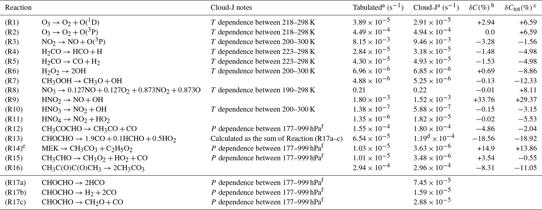
^a Surface clear-sky photolysis rates on DOY 182 at 12:00 LT at 45^∘ N and 15^∘ E. ^b Change in daily mean concentration (%) after 3 d of integration when only the reaction rate specific to each row is changed to Cloud-J. ^c Change in daily mean concentration (%) after 3 d of integration when Cloud-J photolysis rates are used for all photolysis reactions. ^d In EmChem19 the product of glyoxal (CHOCHO) photolysis is based on a fixed relative strength assumption of the R17a–c channels. Here the net photolysis rate from Cloud-J is taken as the sum of R17a–c. ^e Methyl ethyl ketone (MEK = CH₃C(O)CH₂CH₃) assumes α=0 for the CH₃ + C₂H₅CO photolysis product channel described in Zborowska et al. (2021). ^f This range in pressure is tied to a tropical lapse rate, thereby representing an interpolation both in pressure and temperature.

2.4.1 EmChem19

The default EmChem19 chemical mechanism of the EMEP model succeeds the EmChem16 (EMEP status report, 2017) and EmChem09 (Simpson et al., 2012) mechanisms. A key feature of EmChem19 is its aim to balance computational complexity with realism by using a simplified set of surrogate VOCs, as discussed in detail in Bergström et al. (2022). In the context of the current work, notable features of EmChem19 are its 16 primary photolysis reactions, here referring to those reactions which are specific to a certain reactant. Secondary reactions are taken to be those reactions where photolysis rates from one of the primary reactions are used as a (scaled) surrogate and are not discussed in further detail here. The first column of Table 1 gives an overview of the primary photolysis Reactions (R1)–(R16) in EmChem19. The second column gives additional information on the temperature and pressure dependence of the photolysis rates calculated by Cloud-J. While the focus in the current work is on the default EmChem19 mechanism, a brief overview of the Cloud-J implementation in the Common Representative Intermediates (CRI) Version 2 Reduced variant 5 (CRI v2-R5, Watson et al., 2008) chemical mechanism is included in Appendix A1.

The molecular data distributed along with the standard Cloud-J code are used for the photolysis rate calculations for Reactions (R1)–(R15), which is based on quantum-yield and cross-sectional data recommended by Sander et al. (2011) for Reactions (R1)–(R13). For Reactions (R14) and (R15), the molecular data are based on the recommendations of Atkinson et al. (2008). However, Cloud-J is used to extend EmChem19 by explicitly specifying the three glyoxal (CHOCHO) photolysis channels Reaction (R17a–c). In addition, the Cloud-J data are extended for the photolysis of biacetyl (Reaction R16). For this, cross-sectional data between 206 and 496 nm at 1 bar and 298 K from Horowitz et al. (2001) are used, along with an effective quantum yield of ϕ=0.158 between 290–470 nm Plum et al. (1983). The quantum yield is assumed to be zero for wavelengths outside of the 290–470 nm range, as > 99 % of the photodissociation occurs in the 340–470 nm absorption band (Plum et al., 1983).

To test the sensitivity of EmChem19 to the updated photolysis rates, boxChem simulations are run for the 1 July at 45^∘ N and 15^∘ E, corresponding roughly to summertime central Europe. Following the boxChem setup of Bergström et al. (2022, Table 3.1), background mixing ratios for CH4, CO, and H₂ are set to 1800, 120, and 400 ppb, respectively. The atmospheric temperature is set to 298.15 K, with a RH of 66.5 %. A mixing height of 1 km is assumed for the vertical dispersion of emissions. Anthropogenic NO_x and VOC emissions are kept constant at a rate of 18.3 and 15.4 $\mathrm{kg}{\mathrm{km}}^{-\mathrm{2}}{\mathrm{d}}^{-\mathrm{1}}$, respectively, similar to those used by Jenkin et al. (2017, 2008) and Watson et al. (2008). These emissions lead to a simulated daily averaged NO_x mixing ratio of approximately 2.5 ppb, broadly matching observed background surface concentrations over continental Europe. The model is run for a period of three days, after which time daily mean concentrations of the photolyzed species are calculated.

The third and fourth columns in Table 1 show the calculated tabulated and Cloud-J surface photolysis rates at 12:00 LT, respectively, as an indication of the photolysis strength. The fifth column (δC) shows the change in daily mean concentration of the photolyzed species when only the photolysis rate specific to the reaction in each row is changed to Cloud-J. The sixth column (δC_tot) shows the change in concentration when all photolysis rates are changed to those from Cloud-J. The difference between δC and δC_tot thus illustrates that, while the photolysis strength of a single reaction may be higher or lower in Cloud-J, the net impact of the Cloud-J rates may yield a different net change due to the interlinked chemistry. This is illustrated by Reaction (R6), where direct photolysis is reduced, whereas the net concentration change is negative.

Table 1 illustrates that the net change in the daily mean concentrations due to the photolysis rate update is generally on the order of ± 5 %–10 %. Exceptions occur for Reactions (R9) and (R13), which see a net change of 29.4 % and −18.9 %, respectively, owing largely to the changes in their direct photolysis. We note that the standard Cloud-J code treats the ratios of NO and NO₂ production by Reaction (R8) as 0.114 and 0.886, respectively, whereas this ratio is 0.127 and 0.873 in EmChem19. However, using boxChem the different ratios are found to impact simulated NO_x and O₃ concentrations by no more than 0.1 %, such that the default EmChem19 ratio is kept by default. In addition, Table 1 illustrates that the daily mean concentration for biacetyl (Reaction R16) is reduced by 8.31 %, even though the noontime Cloud-J rate is only 0.68 % greater than the tabulated value. However, further analysis finds that the diurnal cycle in Cloud-J is broader than in the tabulated scheme, with reaction rates being higher by 5.9 % on average over the course of the day.

Table 2 Photolysis and cloud field model configurations for the ATom-1 data comparison.

^a includes cloud fraction (CF) and cloud ice and liquid water path (WP). ^b approximates cloud optical depth (OD) in single-column atmosphere grid cell as OD(in-cell) = OD(in-cloud) × ${\mathrm{CF}}^{\mathrm{3}/\mathrm{2}}$ (Briegleb, 1992).

3 ATom-1 aircraft campaign

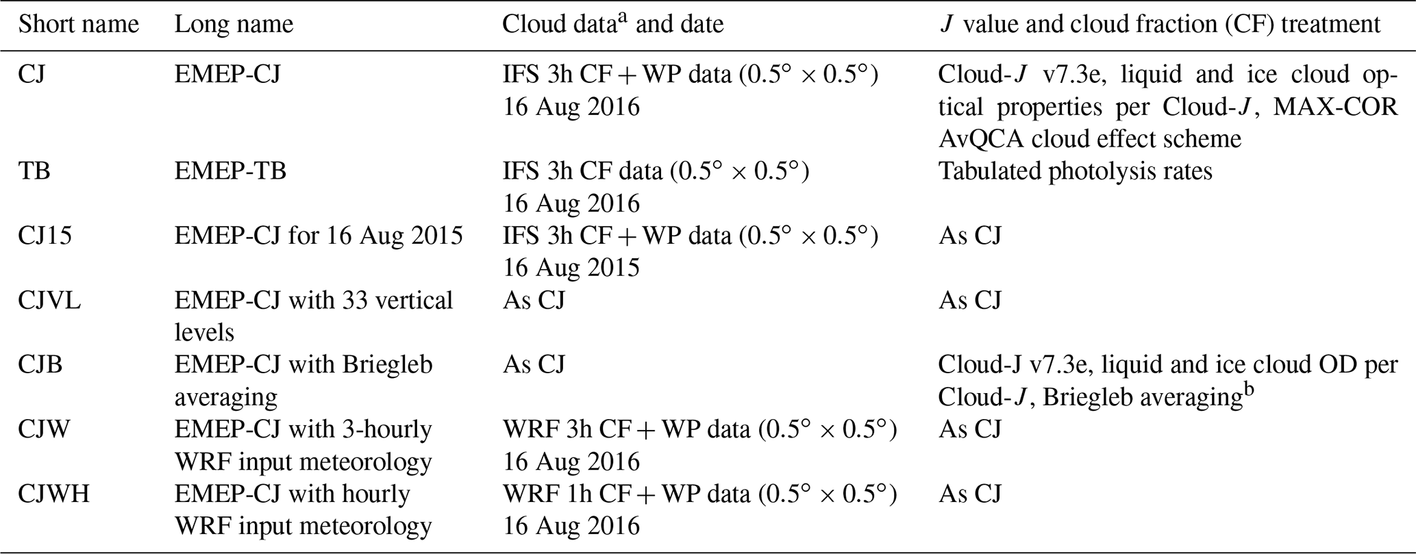
In this section, simulated photolysis rates are compared against observations from the first NASA Atmospheric Tomography (ATom-1) aircraft mission over the Pacific Ocean (Wofsy et al., 2021). During this mission, J-O(¹D) (Reaction R2) and J-NO₂ (Reaction R3) were calculated using the Charged-coupled Actinic Flux Spectroradiometer (CAFS) instrument on board the NASA DC-8 research aircraft (Travis et al., 2020). The CAFS instrument measured 4-π steradian actinic flux density spectra from 280 to 650 nm, with a sampling resolution of three seconds. The analysis discussed here follows that of Hall et al. (2018), who describe the observational data set in detail, along with the methodology to compare the data against photolysis rate calculations from global CTMs. In the current work, comparisons are made against seven diagnostic EMEP simulations, designed to test the sensitivity of the calculated photolysis rates to different model configurations. An overview of the diagnostic model configurations discussed in this section is given in Table 2.

The ATom-1 deployment consisted of 10 flights between the 29 July to the 23 August 2016, occurring mostly during daytime. As described in Hall et al. (2018), the flight data were used to construct a climatological statistic of the observed photolysis rates and cloud effect over the tropical (20^∘S–20^∘ N, 160–240^∘ E) and North (20–50^∘ N, 170–225^∘ E) Pacific blocks for cos (SZA)>0.8. Here the cloud effect refers to the general tendency of clouds to increase photolysis rates above the cloud layer due to scattering while diminishing them below the cloud layer due to shadowing. While the CAFS instrument measured all-sky (for an atmosphere that may contain both clouds and aerosols) photolysis rates during flight time, a conjugate artificially cleared data set of clear-sky photolysis rates was constructed using the Tropospheric Ultraviolet and Visible (TUV) radiative transfer model.

3.1 Vertical profiles

Following Hall et al. (2018), global simulations spanning 24 h on a day in mid-August are used to infer the statistical properties of the simulated J-O(¹D) and J-NO₂ values. To match the CAFS observations, only model data for where cos (SZA)>0.8 are used, for the geographical areas spanning the tropical and North Pacific blocks. Simulations are performed for both all-sky and clear-sky conditions, where the clear-sky simulations also exclude the effect of aerosols. However, consistent with the findings of Hall et al. (2018), diagnostic simulations find aerosols to have a negligibly small impact on the calculated photolysis rates over the Pacific Ocean. While Hall et al. (2018) compare CAFS against model data for simulations anywhere between 15–17 August and the years 2013 to 2017, the EMEP simulations center on the 16 August 2016.

The baseline EMEP-CJ simulation (CJ, in short) uses the model configuration outlined in the Sect. 2.1. The CJB experiment uses the Briegleb averaging rather than MAX-COR AvQCA cloud effect scheme, to investigate the impact of using a less numerically demanding cloud effect scheme (as discussed in Sect. 2.3). An EMEP-CJ simulation for the 16 August 2015 (CJ15) is included to investigate the impact of year-to-year meteorological variability on the constructed photolysis rate statistics. In the CJVL experiment, all IFS vertical levels above the lowest EMEP layer are used from the input meteorology, amounting to a 2-fold increase over the standard number levels, and a corresponding 2-fold increase in the vertical resolution of the cloud field. The EMEP-TB model is included (TB) to provide reference to the tabulated scheme. In addition, EMEP-CJ simulations using input meteorology from the Weather Research and Forecast model (WRF) version 4.4.2 are included (CJW), which has been used to drive the EMEP model in a number of studies (e.g., Ge et al., 2022; Langford et al., 2022; van der Swaluw et al., 2021). The CJW experiment employs the same grid and temporal resolution as those based on the IFS meteorology, whereas the CJWH experiment uses hourly WRF input files instead. The latter experiment investigates the impact of the temporal resolution, noting that hourly data are not available from the IFS input meteorology for the EMEP model. In the current work, the WRF winds and temperatures are nudged to ERA5 reanalysis fields (Hersbach et al., 2020). While the ERA5 model is itself an IFS-based system, the WRF model nevertheless outputs a broad range of other resolved parameters while also employing its own microphysics scheme (WRF-single-moment-microphysics class 5 (WSM5) with ice and supercooled water and snow melt, Hong et al., 2004). To isolate the impact on the photolysis rate calculations, all of the above diagnostic simulations are initialized starting from EMEP-CJ on the 15 August 2016.

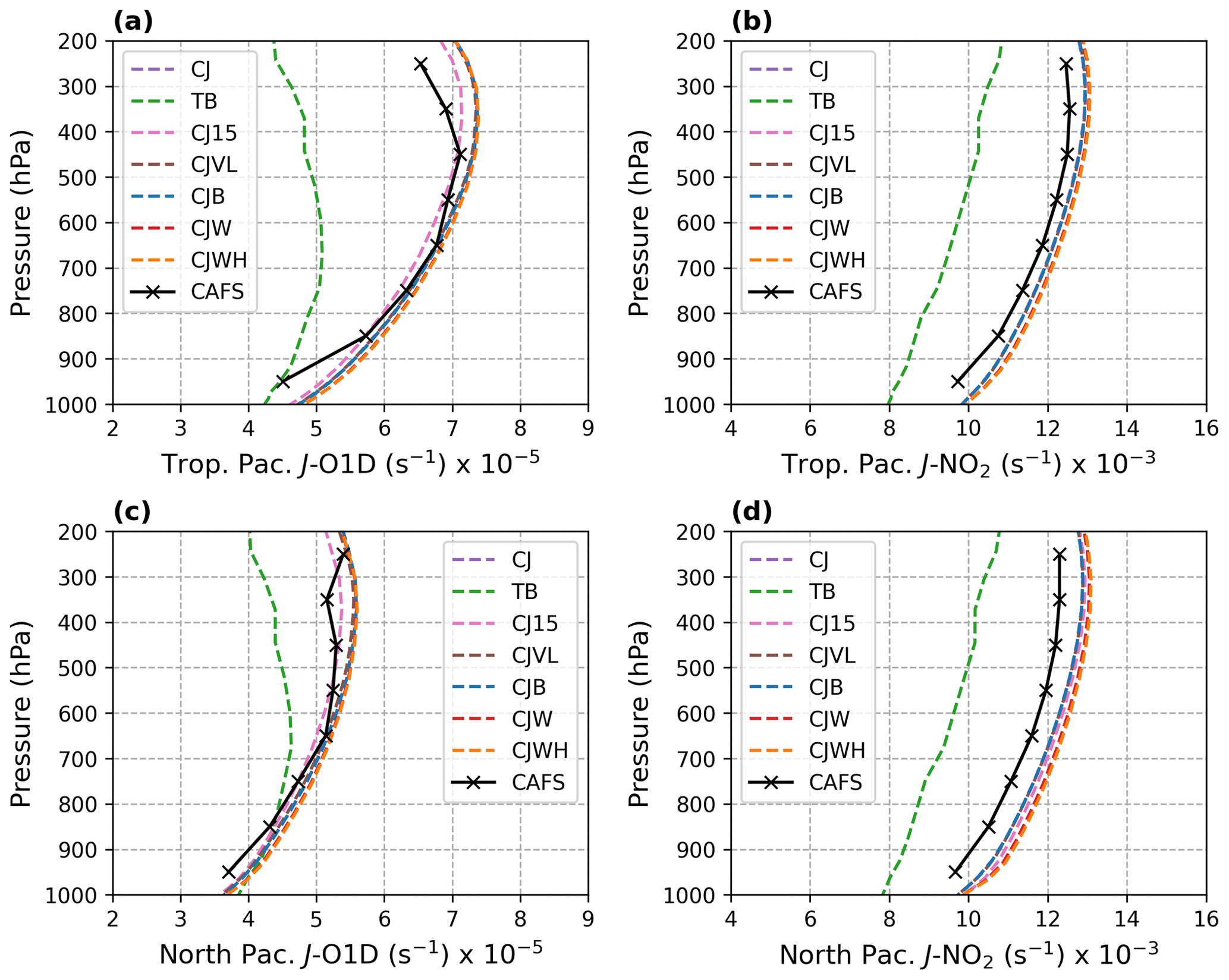
Figure 1 Vertical profiles of clear-sky J-O(¹D) and J-NO₂ over the tropical and North Pacific blocks. The CAFS values are directly measured in ATom-1, while the models are sampled over 24 h on a mid-August day for cos (SZA)>0.8. Legend labels are explained in the text. Note that the x axis does not start at zero.

Figure 1 shows the model and CAFS comparison for the clear-sky photolysis rates. Focusing first on the Cloud-J model configurations, both the simulated and observed photolysis rates maximize towards the upper troposphere, where incoming solar radiation is at its strongest. The calculated clear-sky rates are further nearly identical between the different Cloud-J model configurations, with the exception of the slight deviations present in the J-O(¹D) rates in the CJ15 experiment. All Cloud-J derived photolysis rates are nevertheless within 15 % of the CAFS observations at all altitudes. The TB simulation is markedly different, however, underestimating J-O(¹D) and J-NO₂ over both the tropical and North Pacific basins by as much as 30 %–35 % in the middle and upper troposphere, with the difference being greatest in the tropics.

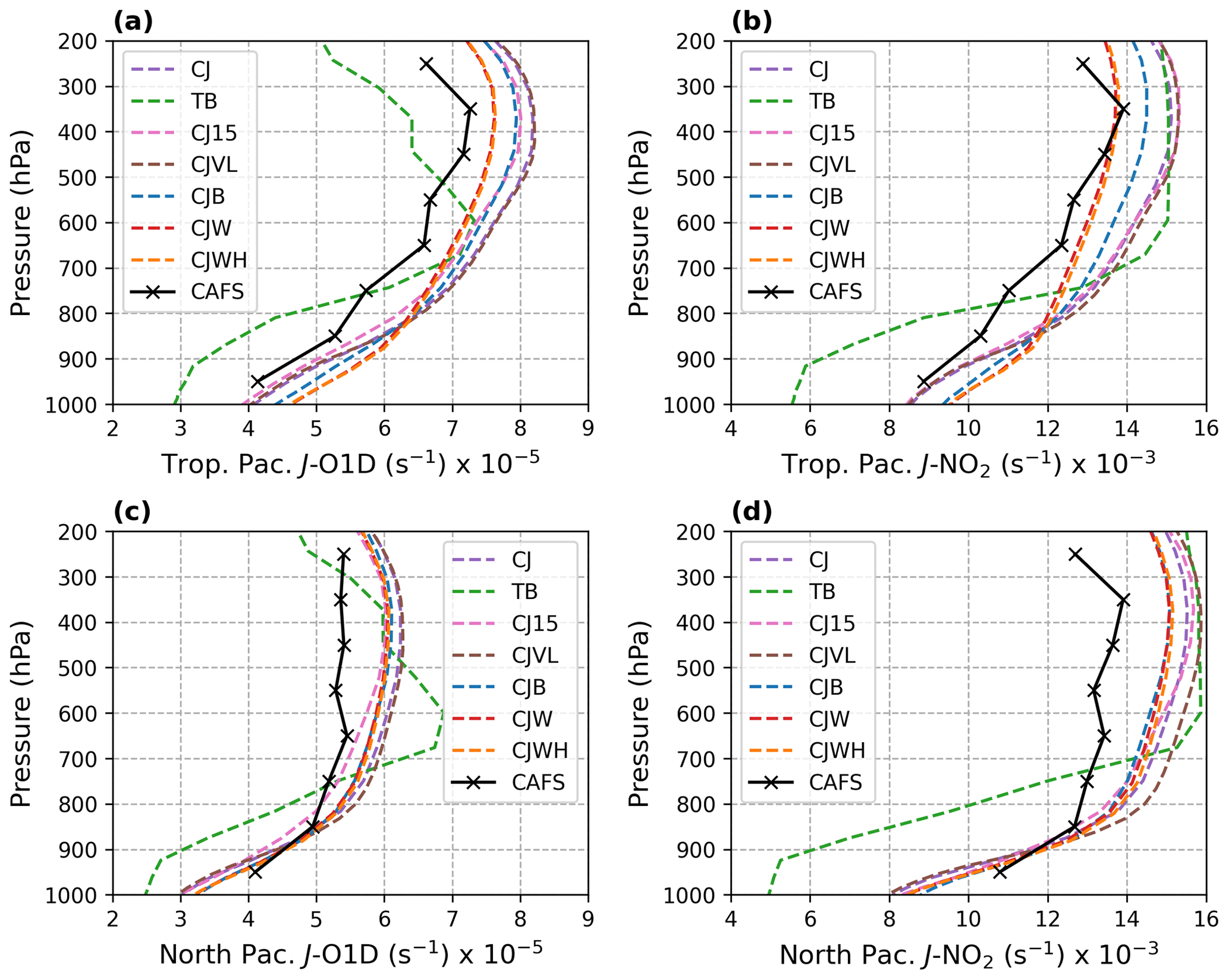
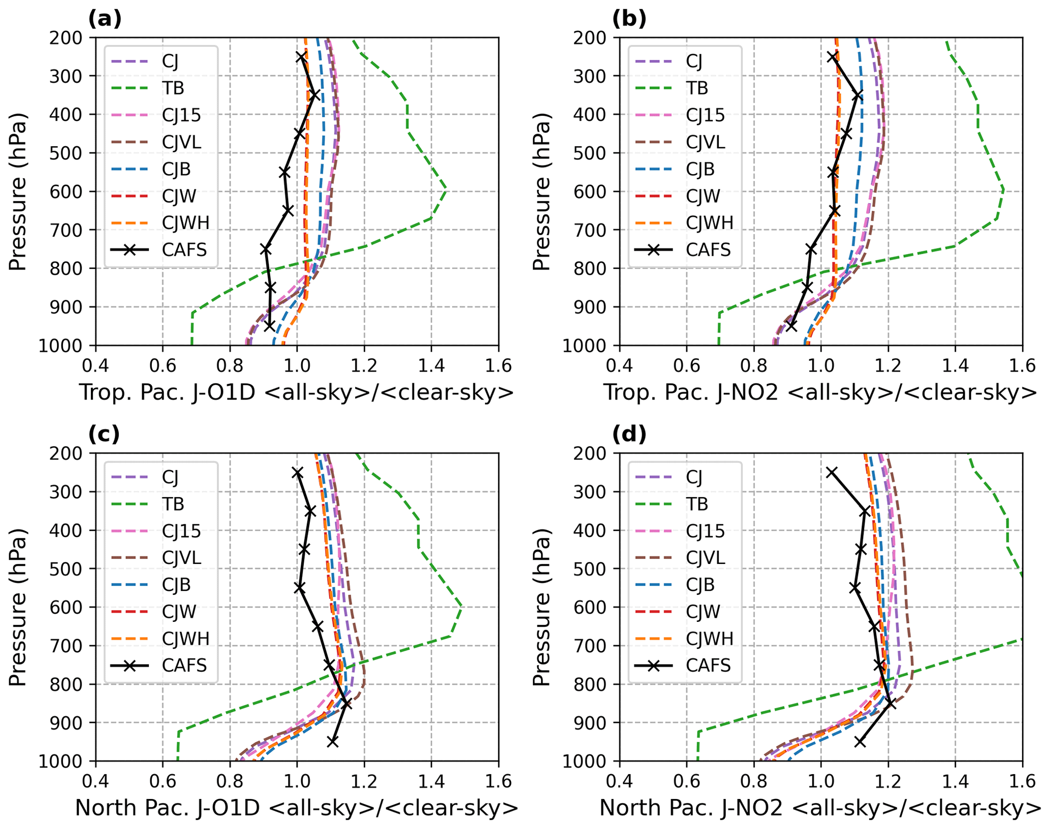
Figure 2 Vertical profiles of all-sky J-O(¹D) and J-NO₂ over the tropical and North Pacific blocks. The CAFS values are directly measured in ATom-1, while the models are sampled over 24 h on a mid-August day for cos (SZA)>0.8. Legend labels are explained in the text. Note that the x axis does not start at zero.

Figure 2 shows the CAFS all-sky photolysis rate comparisons. While the different IFS-based Cloud-J simulations show relatively little inter-model variations, the comparatively largest variations between these modeled J values occur for (1) CJB for J-NO₂ in the tropical Pacific block, (2) both CJB and CJVL for J-NO₂ in the North Pacific block, and (3) CJ15 for J-O(¹D) in both blocks. The largest difference between the Cloud-J simulations occurs for the WRF-based simulations, which generally show lower (higher) photolysis rates above (below) ∼ 800 hPa compared to the IFS-based results. The CJW and CJWH results are nearly identical, indicating that the temporal resolution makes a comparatively small impact. The largest contrast occurs for the TB simulation, whose J values below ∼ 800 hPa are considerably smaller than observation, and much greater than observation for J-O(¹D) in the North Pacific block between 500–700 hPa. For J-NO₂, the TB values are closer to those of the other models, but only for altitudes above 700 hPa. Furthermore, while the CJB results represent a comparatively large deviation from the more accurate CJ solution (given the IFS-based cloud distribution), the impact of using CJB on the EMEP simulation results will be discussed in more detail in Sect. 5.3.

Figure 3 Vertical profiles of the ratio of clear-sky to all-sky J-O(¹D) and J-NO₂ over the tropical and North Pacific blocks. The ratios are calculated based on the data shown in Figs. 1 and 2. Legend labels are explained in the text.

To highlight the impact of the cloud effect, Fig. 3 shows the ratio of the clear-sky to all-sky photolysis rates. In the EMEP-CJ configurations with IFS meteorology, clouds enhance J values by approximately 10 %–20 % above ∼ 800 hPa while diminishing them by 10 %–20 % closer to the surface. Their respective vertical profiles show general agreement with those derived from CAFS, with the exception of the above-cloud enhancement being stronger in the tropical Pacific. For the latter, the CAFS J values are reduced up to an altitude of 500–700 hPa, whereas the simulated rates are reduced only up to altitudes below ∼ 900 hPa. This is in line with the general result that the cloud effect is stronger in the IFS-based Cloud-J simulations than observation, with the CAFS ratios being closer to 1 throughout much the atmospheric column. One caveat is that the ATom-1 aircraft was unable to fly in the marine boundary layer under thick cloudy conditions due to flight safety restrictions, causing the CAFS measurements to have higher than average 950 hPa J values. The latter may in part explain why the sign of the cloud effect is opposite between the simulations and CAFS for the North Pacific below 900 hPa. However, since a below-cloud enhancement has no physical basis in the current models, the difference in sign can also hint at possibly missing modeled cloud field types (Hall et al., 2018).

The cloud effect in the TB simulation stands out as being much stronger than in CAFS or any of the other simulations, both for J-O(¹D) and J-NO₂.

3.2 Cloud effect statistics

Another point of view for the comparison of model and observation is to look at the properties of the distribution of the cloud effect. To this end, the statistics of how often and by how much clouds either increase or diminish the clear-sky J-O(¹D), and J-NO₂ values are calculated for three different vertical regions. The latter are chosen to be representative of the below-cloud, in-cloud, and above-cloud layers, spanning the surface to 900, 900–300, and 300–100 hPa, respectively. As the North Pacific is in general more cloudy than the tropical Pacific, only the results for the North Pacific are discussed in the following. These results are, however, also representative of the tropical Pacific, which is included for reference in Fig. S1 of the Supplement.

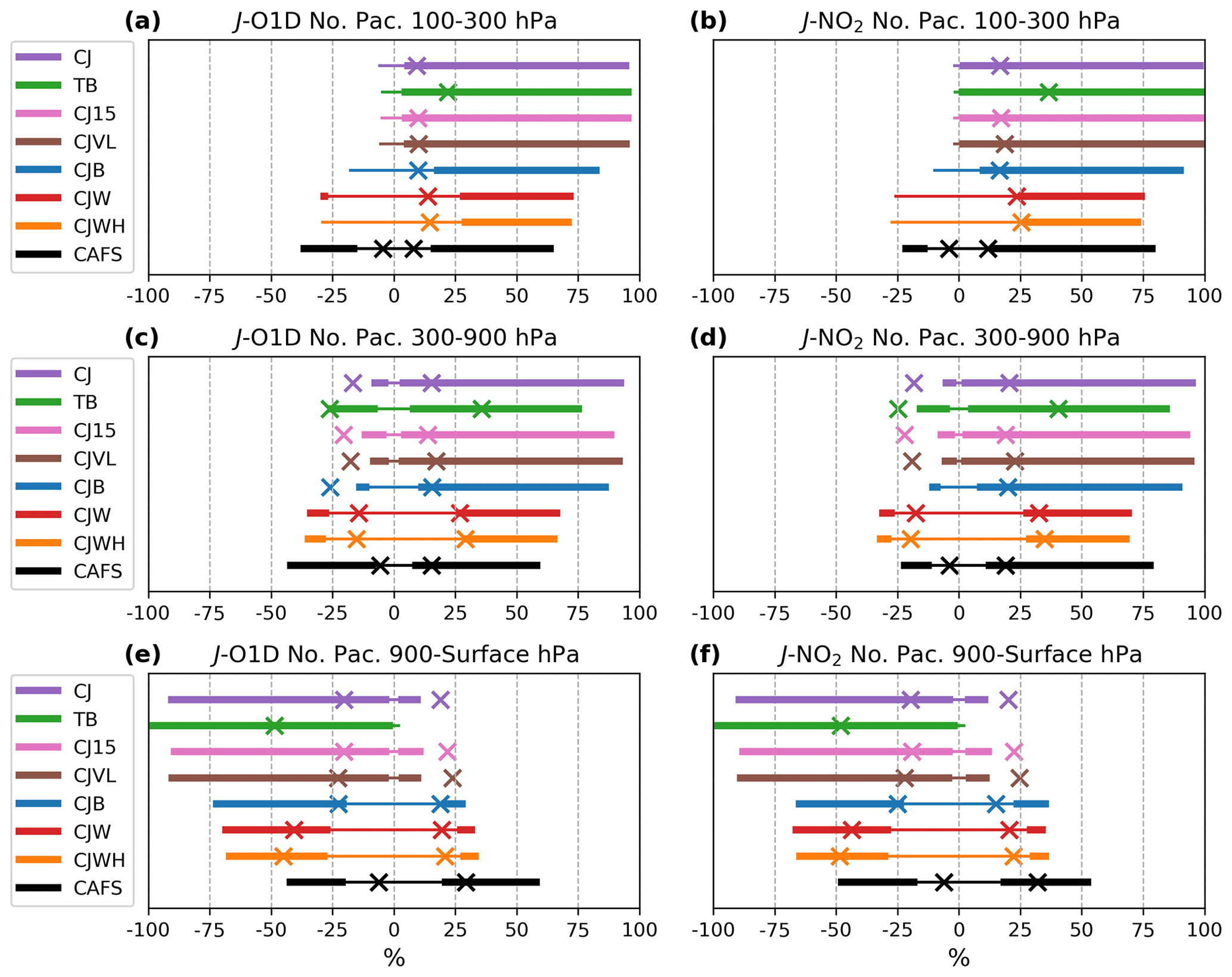
Figure 4 Frequency of occurrence and magnitude of the J-O(¹D) (a–c) and J-NO₂ (d–f) change due to clouds for the below-cloud, in-cloud, and above-cloud tropospheric regions over the North Pacific basin. The interpretation of the line segments and marker locations is explained in the text, as are the legend labels.

Following the approach of Fig. 5 from Hall et al. (2018), the cloud statistics are summarized in Fig. 4 for the CAFS observations and for the different model configurations. In this figure, each of the horizontal bars has a length of 100 %, while the length of the left-most thick segment marks the percentage of measurements for which photolysis rates are diminished by more than 2.5 % by clouds. Similarly, the length of the right-most thick line marks the number of percentage points for which clouds enhance the photolysis rates by more than 2.5 %. The length of the middle thin line segment marks the number of percentage points where photolysis rates are neither enhanced nor diminished by more than 2.5 %, with this segment always being centered on zero on the abscissa. The markers (crosses) denote the average decrease (increase) of the photolysis rates, for those times where the rates are decreased (increased) by more than 2.5 %. Crosses are only shown when at least 2 % of the photolysis rates are either enhanced or diminished by more than 2.5 %. For example, clouds decrease (increase) photolysis rates by more than 2.5 % roughly 20 % (50 %) of the time for the CAFS J-O(¹D) measurements between 100–300 hPa as shown in Fig. 4a, causing a decrease (increase) of around 5 % (8 %) on average.

Figure 4 confirms the picture that the IFS-based EMEP-CJ model configurations generally overpredict the occurrence of enhanced (diminished) photolysis rate in the above (below) cloud layer, although this effect is less pronounced for the CJB simulation. The average enhancement factors in the above-cloud layer nevertheless agree well with observation. In general, the WRF-based simulation shows less above-cloud enhancement and less below-cloud dimming than the IFS-based Cloud-J simulations, while its average enhancement and dimming are stronger. For the in-cloud statistics, all models overestimate the magnitude of the dimming while underestimating its occurrence, while the WRF-based simulations also overestimate the average magnitude of the enhancement. Also here, the CJW and CJWH simulations show nearly identical results. Overall, for the Cloud-J-based simulations, the impact of the vertical resolution and meteorological year is small, while the impact of using WRF meteorology over IFS is considerably larger. Furthermore, for the below-cloud layer the impact of using Briegleb averaging is similar to that of using WRF meteorology. We note that the over-occurrence of above-cloud enhancements is consistent with the tendency of the IFS model to overestimate high-cloud cover and ice water content (Bouniol et al., 2007).

The TB simulation stands out in that its cloud statistic greatly overestimates the occurrence and intensity of both above-cloud enhancements and below-cloud dimming. While the in-cloud frequency of occurrence for both dimming and enhancements provides a reasonable match with observation, the average intensity of these effects is much larger than observed.

Table 3 Diagnostic model configurations for the comparisons to surface observations.

4 Surface observations

In this section, photolysis rate simulations are compared against surface measurements from the Chemistry–Aerosol Mediterranean Experiment 2013 (ChArMEx) in Lampedusa, CYprus PHotochemical EXperiment 2014 (CYPHEX) in Cyprus, and the Chilbolton site in England. Notable differences between these data sets are that the ChArMEx and CYPHEX campaigns took place during near-clear-sky summertime conditions, whereas the Chilbolton measurements took place during cloudy wintertime conditions. A number of diagnostic model simulations are also included in this section, as listed in Table 3.

4.1 ChArMEx 2013

During the ChArMEx 2013 campaign, surface J-O(¹D) and J-NO₂ measurements were made at the ENEA Station for Climate Observations on the island of Lampedusa (35.5^∘ N, 12.6^∘ E). The Lampedusa site, situated on a cliff at about 45 m above sea level on the northeastern tip of the island, is considered a background site with relatively few sources of anthropogenic air pollution (Becagli et al., 2017; Calzolai et al., 2015; Casasanta et al., 2011). The measurements took place between DOY 157 (6 June) and DOY 186 (6 July) of 2013, with a detailed description of the campaign given by Mallet et al. (2016). Atmospheric conditions within the Mediterranean basin and adjacent regions were characterized by lower than average temperatures and limited biogenic and biomass-burning aerosol emissions during the campaign. Moderate aerosol mass concentrations were observed at the Lampedusa site, with PM₁₀ having an average value of 21 µg m⁻³ over the course of the campaign (Mallet et al., 2016). Diagnostic EMEP-CJ simulations find the impact of aerosols on the simulated photolysis rates to be small, showing an average noontime dimming of 1.5 %. Furthermore, monthly mean cloud cover values for June 2013 were below 40 % along the Mediterranean coast near Lampedusa, in agreement with the full time series of observed photolysis rates showing little evidence of cloud effects (Fig. S2).

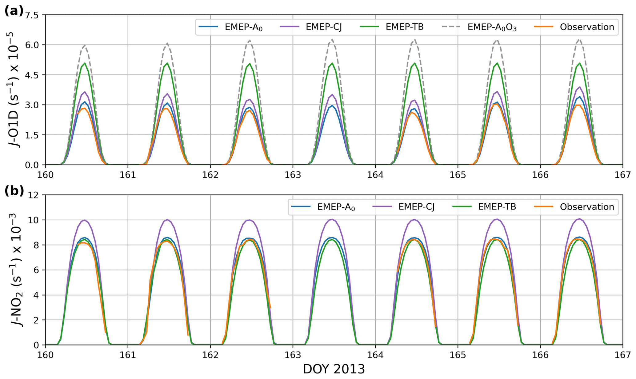
Figure 5 Hourly mean J-O1D (a) and J-NO₂ (b) photolysis rates observed at the Lampedusa site and simulated by EMEP-CJ and EMEP-TB model configurations between DOY 160 and 167 for the year 2013. The EMEP-A₀ simulation includes only the contribution from the downwelling surface actinic flux. In panel (a), EMEP-A₀O₃ represents an EMEP-A₀ simulation where the contribution of the below-100 hPa O₃ column is excluded in the photolysis rate calculations.

A detailed overview of the instrumentation used to measure J-O(¹D) and J-NO₂ is given by Casasanta et al. (2011). In brief, downwelling actinic flux measurements from a METCON diode array spectrometer (DAS, Edwards and Monks, 2003) were used to measure the photolysis rates at 0.5–5 s integration times for local times between sunrise and sunset. A 2-π input optics device was used to send incident photons to the spectroradiometer. The optics device was equipped with a matt-black shadow ring while also applying a stray-light correction. The 1σ uncertainty was less than 10 % for actinic fluxes below 300 nm and less than 3 %–4 % in the 300–340 nm range. The cross-section and quantum-yield data used to derive the J-O(¹D) and J-NO₂ values from the actinic flux measurements are described in Casasanta et al. (2011) and Mailler et al. (2016), respectively. For the measurement-to-model comparison, the observations are averaged in hourly bins matching the averaging periods of the model output. Model output is sampled at the grid box most closely representing the location of the measurement site. Further, since only photolysis by the downwelling actinic flux is measured, Cloud-J photolysis rate calculations where the surface albedo is set to zero (EMEP-A₀) are also included. It is worth noting that this does not consider the portion of the upwelling radiation redirected into the downwelling field from atmospheric scattering, although this contribution is likely of secondary importance. We also note that the surface albedo is set to zero only for the photolysis rate model output, whereas the photolysis rates used in the chemistry remain unchanged (i.e., non-zero albedo).

Figure 5 shows the comparison against observation for the EMEP-CJ, EMEP-TB, and EMEP-A₀ simulations between DOY 160 and 167. While this represents only a subset of the total measurement data, the results discussed in the following are largely independent of the choice of dates, owing to the generally stable meteorological conditions during the campaign. Nevertheless, a comparison of EMEP-A₀ against the full observational data set is given in Fig. S2 of the Supplement.

Figure 5a illustrates that the observed J-O(¹D) values show considerable variations in their daily maxima. For example, the observed daily maximum is 2.54 and 2.98 × 10⁻⁵ s⁻¹ on DOY 164 and 166, respectively, amounting to a 17.3 % variation. These variations are reproduced by EMEP-A₀, having values of 2.83 × 10⁻⁵ s⁻¹ and 3.39 × 10⁻⁵ on DOY 164 and 166, respectively, amounting to a 19.8 % variation. For all the hours shown in Fig. 5a, EMEP-A₀ overpredicts observation by 6.9 % on average. In the EMEP-CJ simulation, the upward actinic flux from the surface reflection increases surface J-O(¹D) rates by 40.9 % on average and by 14.8 % for the noontime values. The comparison between EMEP-TB and EMEP-CJ shows that the tabulated J-O(¹D) values are considerably larger, with noontime values being greater by 44.2 % on average. We note that, since the surface albedo effect cannot be excluded in the tabulated photolysis rate scheme, the EMEP-TB results are most directly comparable to EMEP-CJ.

Figure 5b compares the simulated and observed J-NO₂ values. Here both the EMEP-A₀ and EMEP-TB simulations closely follow the observed daily variations, which themselves show very little day-to-day variability. The EMEP-A₀ and EMEP-TB are both within 8 % of the observed values on average. However, since the EMEP-TB rates include both the upwelling and downwelling actinic flux components, photolysis from the downwelling flux is likely to be underestimated. The EMEP-CJ simulation produces, as expected, values larger than observations, which do not contain the upwelling component.

4.1.1 TOC impact

In Fig. 5a, EMEP-A₀ Cloud-J photolysis rate calculations where the contribution of the O₃ column below the EMEP 100 hPa model top is set to zero (EMEP-A₀O₃) are also included. The smaller day-to-day variability in this simulation indicates that the daily maximum J-O(¹D) variations in EMEP-A₀ are largely caused by daily variations in the below-100 hPa O₃ column. This is consistent with the variations in the observed and simulated TOC, as shown in Fig. 6. In this figure, TOC measurements made at the Lampedusa site by a Brewer spectrophotometer (Mailler et al., 2016; Meloni et al., 2005) during the ChArMEx campaign are compared against hourly modeled TOC. The orange dots highlight the noontime simulated TOC, showing that this value was highest on DOY 164, coincident with the highest observed TOC and lowest observed and simulated J-O1D values. Similarly, the observed and simulated TOC are at a low on DOY 166, coincident with high observed and simulated J-O1D values. The contribution of the above-100 hPa MEGRIDOP satellite O₃ measurements amounts to 247 DU throughout the time period shown in Fig. 6. The O₃ column below 100 hPa thereby contributes between 20 %–30 % of the TOC in the time period shown here, with the variations themselves likely caused by the variable contribution of lower stratospheric O₃. The much higher J-O(¹D) model values obtained in EMEP-A₀O₃ further highlight the role of total O₃ in modulating surface UV radiation around 310 nm.

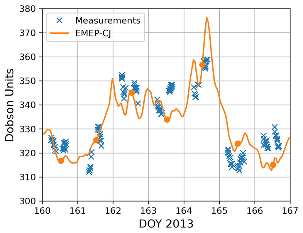
Figure 6 Total O₃ column (TOC) measurements (blue crosses) from the ChArMEx 2013 campaign. The orange line shows hourly total O₃ column values as simulated by the EMEP model appended with MEGRIDOP O₃ data above 100 hPa, with orange circles marking the noontime values.

4.2 CYPHEX 2014

The CYPHEX 2014 campaign took place between July and August 2014 in Ineia, Cyprus, at a measurement site located about 600 $\mathrm{m}\mathrm{a}.\mathrm{s}.\mathrm{l}.$ (35.0^∘ N, 32.4^∘ E). A detailed description of the CYPHEX campaign and measurement site is given by Mallik et al. (2018), Derstroff et al. (2017), and Meusel et al. (2016). In short, downward actinic flux measurements were made using a single monochromator spectral radiometer and 512-pixel CCD array as a detector (275–640 nm), having a total uncertainty of around 10 %. The detector unit was attached to a 2-π integrating hemispheric quartz dome, and photolysis rates for eight of the reactions listed in Table 1 were calculated using the molecular parameters recommended by the International Union of Pure and Applied Chemistry (IUPAC) and NASA evaluation panels (Sander et al., 2011; IUPAC, 2015). In the current work, 10 min measurement data were averaged into hourly bins matching the EMEP model output. Given the prevailing cloud-free conditions and low aerosol concentrations during the campaign (Derstroff et al., 2017), focus is placed on a few days of measurements. Nevertheless, a comparison of EMEP-A₀ against the full observational data set is given in Fig. S3 of the Supplement.

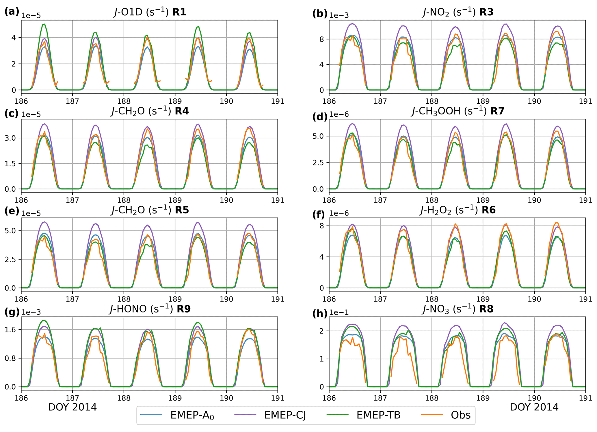
Figure 7 Hourly mean photolysis rates for eight photolysis reactions measured during the CYPHEX 2014 campaign (orange), and as simulated by EMEP-A₀ (blue), EMEP-CJ (purple), and EMEP-TB (green). Plot titles refer to the reactions listed in Table 1.

Figure 7 shows the comparison between observation and the EMEP-CJ, EMEP-A₀, and EMEP-TB simulations between DOY 186 and 191 (8 to 12 July), for the eight measured photolysis reaction rates present in EmChem19. Focusing on J-O(¹D) shown in Fig. 7a first, EMEP-A₀ shows the closest agreement with observation for DOY 186 and 187. For the other days, however, EMEP-CJ is closer to observation. The EMEP-TB values are higher than those simulated by EMEP-CJ and show moderate day-to-day variability attributable to light cloud cover variations in the input meteorology. The impact of the latter is much smaller in the Cloud-J simulations, however, with the calculated photolysis rates showing little day-to-day variability. The other Cloud-J photolysis rates show similarly little day-to-day variation, with the exception of J-NO₃. For the latter, the impact of any (light) cloud or aerosol presence is comparatively the largest both for model and observation, possibly owing to its almost exclusive dependence on wavelengths in the visible spectrum. While EMEP-A₀ provides the general best agreement with observation, EMEP-CJ consistently shows the closest agreement for J-H₂O₂ (Fig. 7f). On average, EMEP-A₀ underestimates J-H₂O₂ by 15.0 % for the time period under consideration.

4.3 Chilbolton

Photolysis rate measurements were made between the 17 December 2020 and 22 March 2023 at Chilbolton Observatory, situated at a rural background air quality monitoring station ∼ 100 km southwest of London (51.1^∘ N, 1.3^∘ W). A detailed description of the Chilbolton site and experimental setup is given in Walker et al. (2022). In short, spectral actinic flux was measured between 280–750 nm with a ∼ 1 nm resolution, using a CCD spectroradiometer coupled with a fiber-optic cable to a single 2-π quartz receiver optic. The station is located 78 $\mathrm{m}\mathrm{a}.\mathrm{s}.\mathrm{l}.$, with the measurement device mounted 6.5 m above ground level on a black-painted cabin roof railing. In addition to a dark signal correction, a stray-light correction was applied to account for any actinic flux originating from the surrounding grass and arable farmland. IUPAC-recommended values for absorption cross-sections and quantum yields were used to derive photolysis rates at a 1 min resolution, which were used to construct a time series of hourly values in the current work. The agreement between CCD spectroradiometer-derived photolysis rates and those measured by a double-monochromator reference instrument was found to be within ± 5 % (Bohn and Lohse, 2017). As before, only those measured photolysis rates that are present in EmChem19 are discussed.

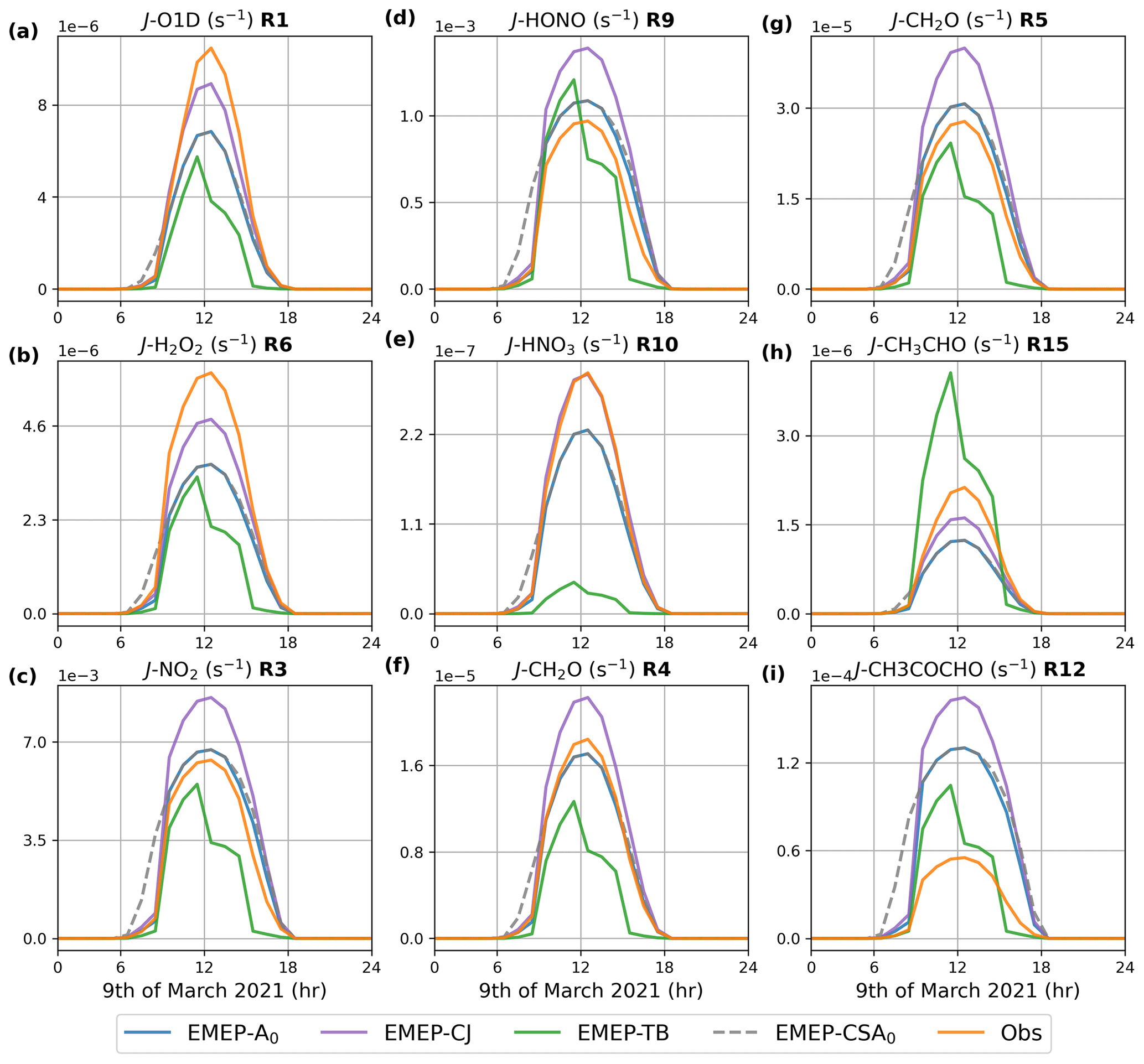
Figure 8 Hourly mean photolysis rates measured at the Chilbolton site (orange) and as simulated by the EMEP-A₀ (blue), EMEP-TB (green), EMEP-CJ (purple), and EMEP-CSA₀ (gray, dashed) model configurations for the 9 March 2021. Plot titles refer to the reactions listed in Table 1.

During the measurement period, 9 March was the day most representative of clear-sky conditions (Walker et al., 2022), with SZAs in the range of 50–60^∘. Figure 8 shows the comparison against EMEP-A₀, EMEP-CJ, and EMEP-TB for this day while also including a comparison against EMEP-A₀ with clear-sky photolysis rates (EMEP-CSA₀). This figure shows that EMEP-A₀ underestimates J-O(¹D), J-HNO₃, J-H₂O₂, and J-CH₃CHO by a considerable margin, with the difference being as large as a factor of 2. The commonality between these photolysis rates is the large influence of absorbance at wavelengths below 350 nm (Walker et al., 2022, Fig. 3), thus suggesting that the photolysis by UV radiation is underestimated. It is unclear whether this model underestimation is the result of, for example, an overestimation of the total ozone column or of overestimated scattering or absorbance in the overhead atmospheric column. The close agreement between EMEP-A₀ and EMEP-CSA₀ shows that cloud cover and aerosols have very little impact on the Cloud-J simulation results, except for the hours between 06:00–09:00 LT. However, the EMEP-TB photolysis rates decrease considerably after 12:00 LT, suggesting that the cloud effect is overestimated in the tabulated scheme.

Figure 8 also shows that EMEP-A₀ overpredicts J-CH₃COCHO (MGLY) by a factor of around 2. This overprediction is similar to the results obtained using the Tropospheric Ultraviolet and Visible radiation model version 5.3 (TUV v5.3) by Walker et al. (2022), finding an overprediction of MGLY by a factor of ∼ 1.5. Since both the EMEP and TUV models employ the same cross-sectional and quantum-yield data as the Chilbolton spectral radiometer, based on Meller et al. (1991) and Chen et al. (2000), respectively, the results for MGLY hint at a possible model shortcoming elsewhere.

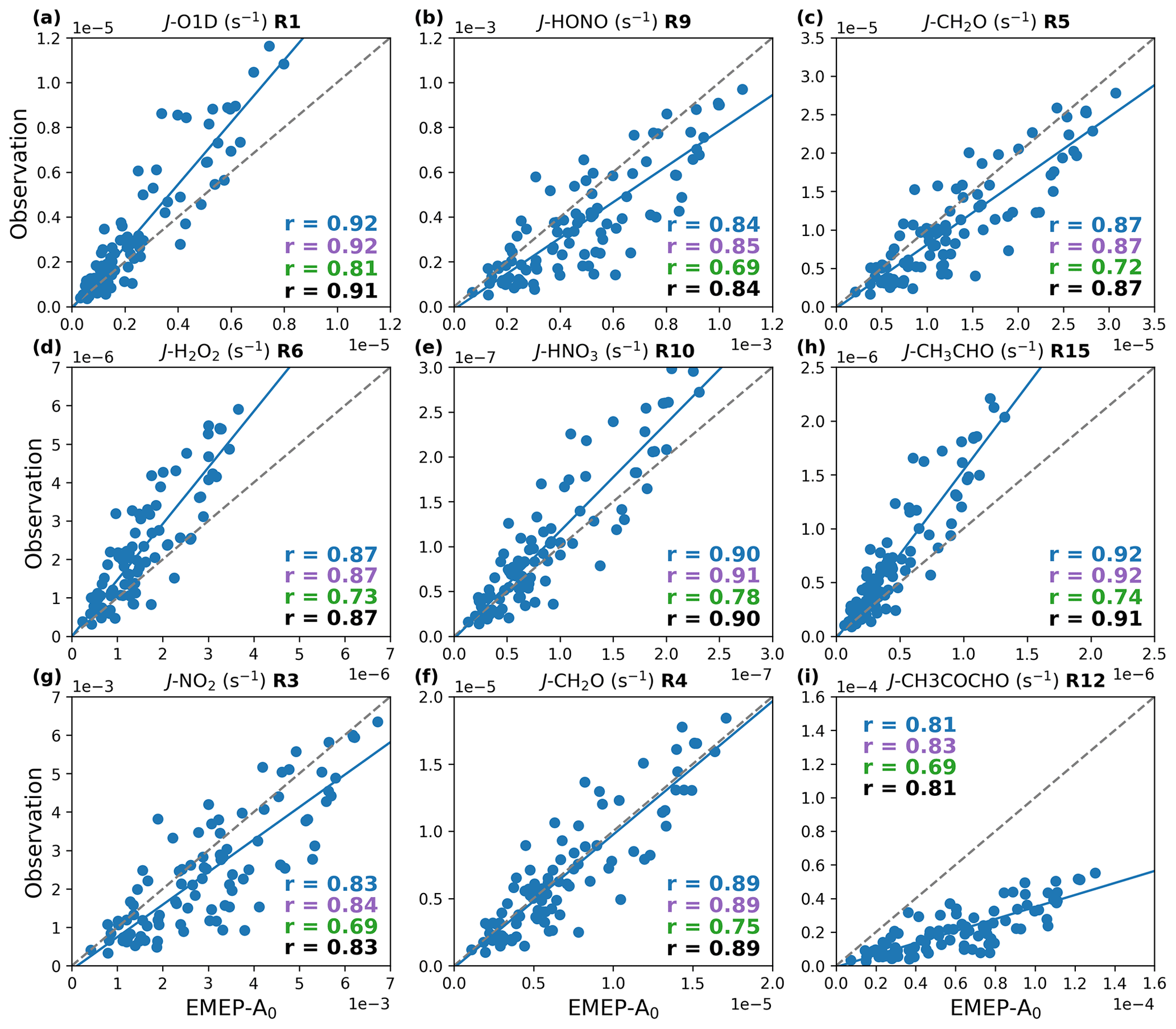
Figure 9 Noontime hourly mean photolysis rates measured at the Chilbolton site and as simulated by EMEP-A₀ (blue) between the 17 December and 22 March 2021. The correlation coefficient (r) for EMEP-A₀, EMEP-CJ (purple), EMEP-TB (green), and EMEP-A₀HR (black) are also shown. Plot titles refer to the reactions listed in Table 1.

As shown in Fig. 2 from Walker et al. (2022) and Fig. S4 of the Supplement, the full time series of observed and simulated photolysis rates display a large degree of day-to-day variability, superimposed on a seasonal variation. The observed day-to-day variations in peak photolysis rate values can largely be attributed to daily variations in local cloud cover and other factors determining cloud optical properties, such as cloud thickness, altitude, and temperature (Walker et al., 2022). In the following, the day-to-day variability is leveraged to investigate the representation of the simulated cloud effect. Figure 9 shows scatterplots of the observed and simulated EMEP-A₀ noontime photolysis rate values, along with their correlation coefficients (r) and linear regression curves, for the 95 d of available data. For reference, the correlation coefficients for the EMEP-CJ and EMEP-TB model configurations are also included. The day-to-day variability in peak photolysis rates is described well in EMEP-A₀, with correlation coefficients in the range of 0.81–0.92. Similar results hold for the EMEP-CJ simulation, while the range of correlation coefficients is considerably lower for EMEP-TB (0.69–0.81). For reference, Fig. S4 also shows the normalized mean bias (NMB, %) with respect to observation for the participating models, illustrating that the average values are considerably lower in EMEP-TB than in EMEP-CJ, with the exception for J-CH₃CHO.

Figure 9 and Fig. S4 also show the correlation coefficient and NMB statistics, respectively, for the diagnostic EMEP-A₀HR simulation. In this configuration, the EMEP-A₀ simulation is repeated on a higher regional 0.1^∘ × 0.1^∘ horizontal grid, leaving the other model parameters unchanged. Given the similarity between the EMEP-A₀ and EMEP-A₀HR results, the factor of 25 decrease in grid-box size is found to have little impact on the photolysis rate calculations. The values of the correlation coefficients differ by no more than 0.01, while the NMB values show differences only on the order of a few percent points. Similar diagnostic analysis finds that the horizontal grid resolution has a similarly small impact on the ChArMEx and CYPHEX measurement-to-model comparisons.

5 Model analysis

This section investigates the impact of the Cloud-J photolysis rates on the EMEP simulations results, using global simulations for the year 2018. To this end, the oxidizing capacity of the troposphere is examined, in addition to the impact of aerosol–photolysis interactions. Model results for EMEP-CJ and EMEP-TB are also compared against surface observations of O₃, CO, and NO₂ across Europe and against surface O₃ observations from four select hemispheric sites.

5.1 Oxidizing capacity of the troposphere

The tropospheric OH budget has historically been an important metric for the inter-comparison of global CTMs (Eastham et al., 2014). Most natural and anthropogenic atmospheric gases are removed through oxidation initiated by OH, with the OH abundance regulating the lifetime of key atmospheric species such as CH4, VOCs, and CO (Lelieveld et al., 2016; Crutzen and Zimmermann, 1991). Photolysis is the main driving mechanism for the production of OH, as the primary production pathway of OH depends on the photolysis of O₃ (Reaction R1, Table 1) and the subsequent reaction of O(¹D) with water vapor. Once produced, approximately 40 % of OH is lost to the reaction with CO (Murray et al., 2021).

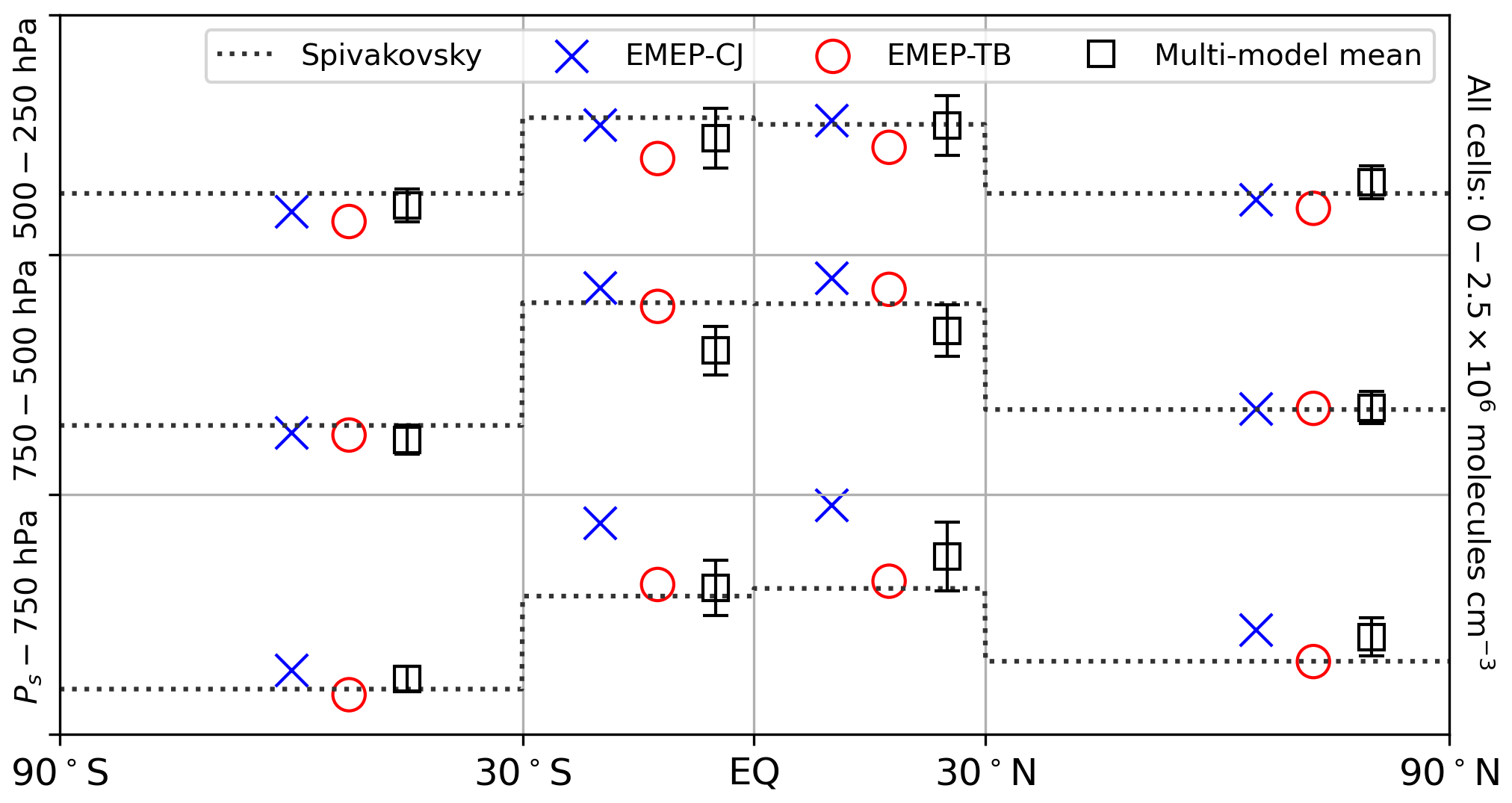
Figure 10 Mass-weighted regional mean annual mean OH concentration from EMEP-CJ (cross), EMEP-TB (circle), the 17 multi-model means and standard deviations from Naik et al. (2013) (square), and reference climatology from Spivakovsky et al. (2000) (dotted). The vertical range of each of the regions extends from 0 to 2.5 × 10⁶ $\mathrm{molec}.{\mathrm{cm}}^{-\mathrm{3}}$.

Following the approach recommended by Lawrence et al. (2001), Fig. 10 shows the air mass-weighted annual mean zonal mean OH budget across 12 tropospheric latitude–altitude sectors. Here, the results for EMEP-CJ and EMEP-TB are shown, along with the results for the 17 global models participating in the inter-comparison study of Naik et al. (2013) for the year 2000. In addition, the reference climatology from Spivakovsky et al. (2000) is included. While the EMEP results are shown for the year 2018, inter-annual variability of the yearly mean global OH abundance is on the order of 1 %–3 % (as inferred by Montzka et al., 2011), making the results representative also of other years of simulation. The numbers corresponding to the results shown in Fig. 10 are also included in Table S1.

Figure 10 shows that both EMEP-CJ and EMEP-TB simulate comparatively low OH concentrations in the mid- and high-latitude upper troposphere (> 500 hPa), having OH concentrations near or less than 1 standard deviation from the 17-model mean. In the tropical upper troposphere, both EMEP-CJ and EMEP-TB fall within 1 multi-model standard deviation, while EMEP-CJ shows the closest correspondence with the reference climatology. For the middle troposphere (750–500 hPa), both EMEP-CJ and EMEP-TB predict concentrations near the reference climatology, whereas the 17-model mean shows considerably lower concentrations in the tropics.

The Cloud-J photolysis rates considerably increase OH relative to EMEP-TB in the tropical lower troposphere (< 750 hPa), with mass-weighted concentrations substantially exceeding the 17-model mean and reference climatology. In contrast, the tropical lower atmosphere results for EMEP-TB are on the lower end of the 17-model results while being close to the reference climatology. This seemingly superior performance of the EMEP-TB model is, however, likely to be the result of its underestimated tropical J-O(¹D) values, as discussed in Sect. 3. EMEP-CJ nevertheless brings the global average mass-weighted OH concentrations (11.67 × 10⁵ $\mathrm{molec}.{\mathrm{cm}}^{-\mathrm{3}}$) close to that of the multi-model mean reported by Naik et al. (2013) (11.16 ± 1.6 × 10⁵ $\mathrm{molec}.{\mathrm{cm}}^{-\mathrm{3}}$), compared to the 9.27 × 10⁵ $\mathrm{molec}.{\mathrm{cm}}^{-\mathrm{3}}$ average from EMEP-TB. For the comparatively high lower tropical OH in EMEP-CJ, possible factors may be related to, for example, water vapor concentrations in the input meteorology, tropospheric ozone concentrations, or tropical CO concentrations (Travis et al., 2020). A detailed investigation is, however, beyond the scope of the current work.

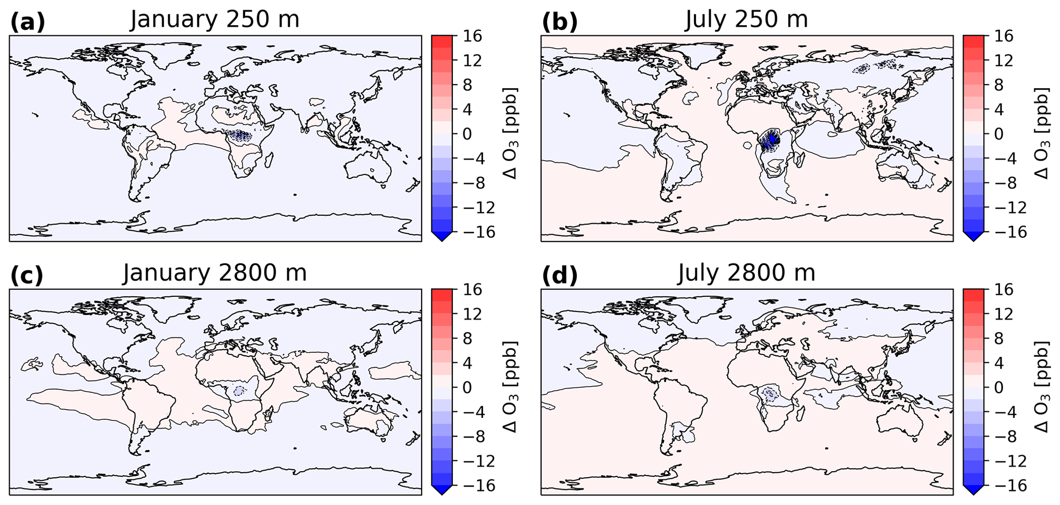
Figure 11 Perturbation to monthly mean O₃ concentrations at 250 and 2800 m altitude in January (a, b) and July (c, d) 2018 due to aerosol photolytic effects.

5.2 Aerosol photolytic effect

Following the approach of Bian et al. (2003), changes to tropospheric O₃ concentrations are used as a marker of the impact of aerosol radiative scattering and absorption on photolysis rates. To this end, monthly mean O₃ concentrations simulated by EMEP-CJ are compared against those simulated by a diagnostic simulation where Cloud-J aerosol radiative effects are turned off (control run). Figure 11 shows the difference between the two simulations at 250 and 2800 m altitude for January and July 2018, calculated as EMEP-CJ minus the control run.

Figure 11 shows that the O₃ perturbation caused by aerosols is largest over the tropical biomass-burning regions. In July, biomass-burning aerosol photolytic effects reduce O₃ concentrations by as much as 12–16 ppb over central Africa. While this impact is a factor of 2–3 stronger than the climatological findings of Bian et al. (2003), the EMEP-CJ region affected by biomass burning is also comparatively more geographically contained, possibly owing to the single year of simulation. In EMEP-CJ, both sea salt and dust impact O₃ by less than 1–2 ppb, which for dust represents a smaller effect than the 3–4 ppb O₃ decrease over the Middle East and parts of southern Europe reported by Bian et al. (2003) for July conditions. While the impact of dust in the EMEP-CJ configuration is smaller than that reported by Bian et al. (2003), the reason for this can be easily obscured by its dependence on the simulated aerosol concentrations, aerosol chemical properties, calculated aerosol optical properties, and radiative transfer scheme (Real and Sartelet, 2011; Kinne et al., 2003). Assessing the importance of the aforementioned effects within the EMEP-CJ model would therefore require a coordinated approach combining other models with a detailed comparison against observed aerosol properties.

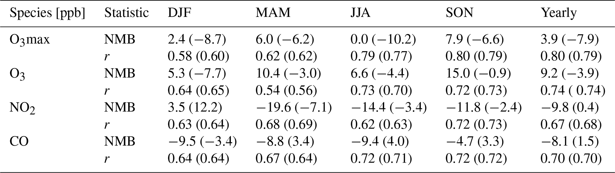
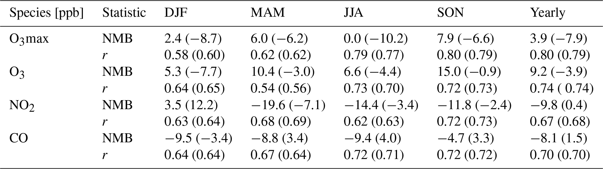
Table 4 NMB (%) and correlation coefficients for EMEP-CJ and EMEP-TB (brackets) against surface observations from the EBAS database in Europe. Statistics are based on daily values and are shown for the four seasons as well as for the yearly average.

5.3 Surface air pollution

In this section, the EMEP-CJ and EMEP-TB models are evaluated against O₃, NO₂, and CO surface observations from the EBAS database (Tørseth et al., 2012). The data used comprise hourly time series from 138 stations for O₃ and daily mean time series from 93 and 8 stations for NO₂ and CO, respectively. The measurement stations are spread across urban, suburban, and rural sites throughout Europe. In addition, the hourly O₃ time series are used to construct a time series of daily O₃max concentrations, being the maximum 1-hourly mean value over the course of a day, which is a commonly used indicator for air quality. Table 4 shows the normalized mean bias (NMB, %) and correlation coefficient between the models and observations for the winter (DJF), spring (MAM), summer (JJA), and fall (SON) seasons, as well as for the annual mean. Here all statistics are averaged over their respective time periods and across all stations, using the measured and modeled daily values. The time series of the data underlying statistics shown in Table 4 is included in Fig. S5 of the Supplement.

Table 4 highlights that O₃ and O₃max concentrations are generally increased in EMEP-CJ relative to EMEP-TB, while NO₂ and CO concentrations are decreased. The use of EMEP-CJ thereby has the clear consequence of partitioning more O_x (= O₃ + NO₂) into the O₃ component. The correlation coefficients are most strongly impacted during the spring and summer seasons, with the correlation coefficients for CO and O₃ seeing the largest increases of 0.03 in spring and summer, respectively. The positive bias in the daily mean O₃, together with the generally low bias for O₃max, indicates that the diurnal variations are underestimated in EMEP-CJ. However, the latter is also apparent in EMEP-TB, where the bias in daily mean O₃ is less negative than that for O₃max. For NO₂, the largest absolute NMB percentage changes occur in spring and summer, with EMEP-CJ considerably underestimating NO₂ concentrations. Note, however, that EMEP-TB also underestimates NO₂ in summer and that EMEP-TB overestimates NO₂ in winter. The NMB for CO is generally increased, even though its correlation coefficient is increased in spring and summer.

Figure 12 highlights the spatial variations in the yearly mean O₃max NMB changes between EMEP-CJ and EMEP-TB. In this figure, the difference between the absolute value of the annual mean NMB at the measurement sites is shown, with decreases (increases) in NMB marked by blue (red) dots. Overall, EMEP-CJ has annual mean O₃max values closer to observation across most of central and eastern Europe, while the performance is decreased in western Spain and the western and northern stations of the United Kingdom and Ireland. The latter are indicative of a possible overestimation of the influx of O₃ carried over the Atlantic Ocean by the surface westerlies, noting that the NMB in these regions is generally greater than zero.

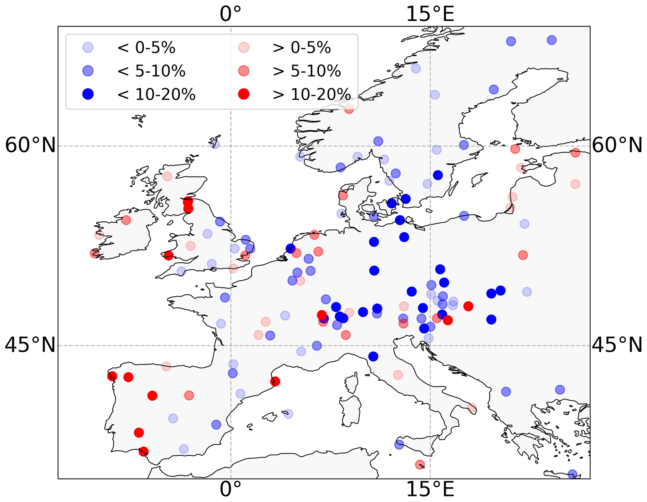
Figure 12 Difference in the absolute yearly mean O₃max NMB (%) between the EMEP-CJ and EMEP-TB simulations relative to surface observations from the EBAS database. Blue dots indicate that the average simulated value is closer to observation in EMEP-CJ than in EMEP-TB, and vice versa for the red dots.

We note that the results presented in this section are largely independent of using either the MAX-COR AvQCA or Briegleb averaging cloud schemes (as discussed in Sect. 2.1), in addition to updating the photolysis rates only once every model hour rather than model time step (EMEP-CJBh, Table 3). Employing model time-step calculations with the MAX-COR AvQCA scheme, the EMEP model run time is increased by roughly 150 % compared to EMEP-TB. Using an hourly update approach combined with Briegleb averaging, however, the run-time increase is only about 15 %. The correlation coefficients and the NMB shown in Table 4 are nevertheless nearly identical for EMEP-CJBh relative to EMEP-CJ, as shown in Table S2 in the Supplement. The correlation coefficients are changed by no more than 0.01, and only for O₃max in summer, while the NMB values are changed by no more than 0.8 % in absolute terms. For reference, the full time series of surface pollutants calculated using EMEP-CJBh is included in Fig. S5. We note that similar results for using either the MAX-COR AvQCA or hourly Briegleb approach also hold for the higher-resolution 0.1^∘ by 0.1^∘ EMEP grid.

5.3.1 Global sites

This section compares simulated daily maximum O₃ concentrations against observations from four Global Atmospheric Watch (GAW; Schultz et al., 2015) stations, from locations representative of four distinct hemispheric air masses. To that end, the Ryori site (39.0^∘ N, 141.8^∘ E) in Japan is chosen as being indicative of O₃ production downwind of mainland China, and the Tudor Hill site (32.3^∘ N, 64.9^∘ W) (Bermuda) is chosen as being indicative of O₃ production downwind from the United States. The seasonal variations at the Mace Head (53.3^∘ N, 9.9^∘ W) (Ireland) and Trinidad Head (41.1^∘ N, 124.2^∘ W) (west coast, USA) stations are taken to be broadly representative of background air masses carried over the North Atlantic and Pacific oceans, respectively (Parrish et al., 2009).

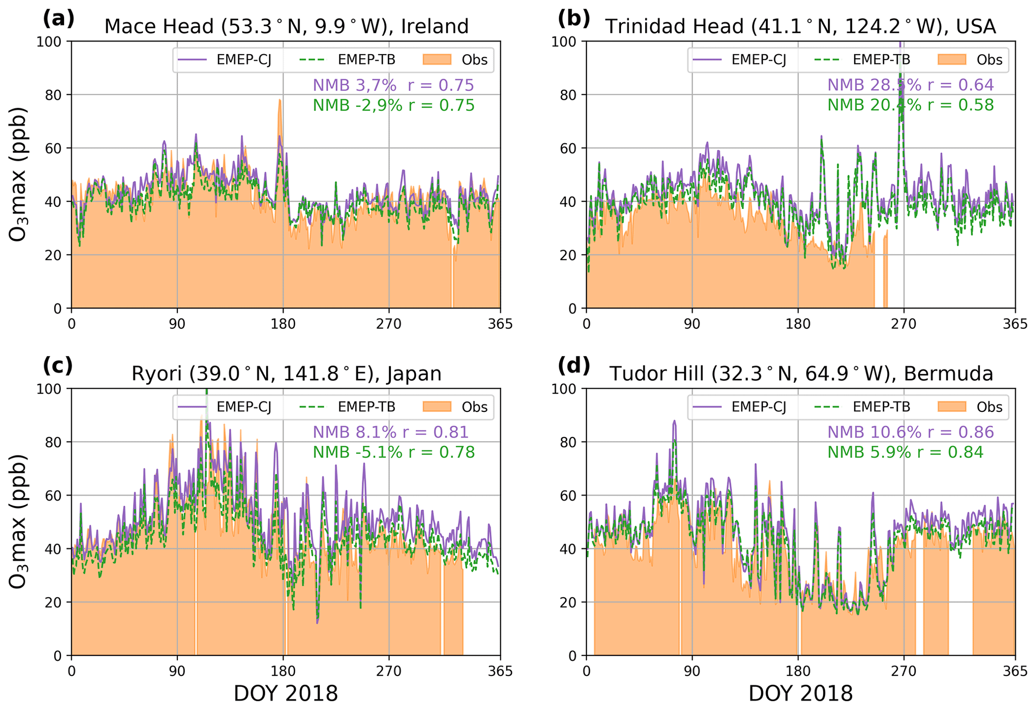
Figure 13 Time series of observed and simulated daily maximum O₃ concentrations at four Northern Hemisphere GAW sites. The shaded area refers to the observed surface station concentrations, whereas the dashed green line refers to EMEP-TB and the purple solid lines to EMEP-CJ. The model NMB (%) and correlation coefficients with respect to observation are shown in each of the panels.

Figure 13 shows the time series of observed and modeled daily maximum O₃ concentrations. The observed seasonal and daily variations are described well in both the EMEP-CJ and EMEP-TB model configurations, although the daily variations during summertime are overestimated at Trinidad Head in both model configurations. Consistent with the results from the previous section, surface O₃max concentrations are generally higher in EMEP-CJ than in EMEP-TB. For the stations upwind and downwind of the United States, this further increases the positive bias present in EMEP-TB. For the Mace Head and Ryori stations, the negative bias of EMEP-TB is replaced by a positive bias of a similar magnitude. EMEP-CJ increases the correlation coefficient by up to 0.06 compared to EMEP-TB, although it remains unchanged at the Mace Head station.

6 Conclusion

This study implemented and evaluated the Cloud-J v7.3 photolysis rate calculation code in the EMEP model. Cloud-J represents a major update with respect to the old tabulated photolysis rate system, offering an improved representation of the cloud radiative effect, in addition to providing a description of aerosol–photolysis interactions. The performance of Cloud-J is established through its favorable and robust comparison against measurements from the CAFS instrument on board the ATom-1 flight campaign over the Pacific Ocean and against surface measurements from the Lampedusa (ChArMEx 2013), Cyprus (CYPHEX 2014), and Chilbolton surface sites. The old tabulated scheme is found to greatly overestimate the cloud radiative effect while also underestimating clear-sky photolysis rates in the tropics. While the general performance of Cloud-J is encouraging, the Cloud-J-based simulations show a tendency to overpredict the frequency of occurrence and magnitude of above-cloud enhancements and below-cloud diminishments (Sect. 3) while also underestimating wintertime photolysis rates sensitive to wavelengths below 350 nm (Sect. 4.3).

Notable results from the sensitivity analysis are that the calculated Cloud-J photolysis rates are comparatively insensitive to the temporal, vertical, and horizontal model resolution. They are instead more strongly impacted by the difference in the cloud field representation between the IFS and WRF models and to a lesser extent by the choice of cloud effect scheme between the MAX-COR AvQCA and Briegleb averaging schemes. However, using the comparatively less computationally expensive Briegleb averaging scheme, together with hourly photolysis rate updates, is found to have a negligibly small impact on the EMEP simulation results while keeping the total model run-time increase below 15 %. In the comparison to the Lampedusa surface observations, diagnostic simulations further find that daily variations in the total O₃ column induce up to 17.3 % (19.8 %) variations in measured (modeled) day-to-day maximum surface J-O(¹D) values.

The model results with Cloud-J enabled show an improvement in the average correlation and NMB statistics with respect to observed surface daily maximum O₃ concentrations in Europe. The model bias for surface NO₂ is significantly worsened during spring, however, possibly hinting at model shortcomings elsewhere, given the improvement in J values. In addition, a negative bias for surface CO is introduced, even though its correlation coefficient increases during the spring and summer seasons. The comparison against four northern hemispheric background surface measurement sites confirms the finding that using Cloud-J leads to generally higher simulated surface O₃ concentrations across the Northern Hemisphere. On a global scale, Cloud-J increases the annual mass-weighted tropospheric OH budget from 9.27 × 10⁵ to 11.67 × 10⁵ $\mathrm{molec}.{\mathrm{cm}}^{-\mathrm{3}}$, bringing it in line with the 11.12 × 10⁵ $\mathrm{molec}.{\mathrm{cm}}^{-\mathrm{3}}$ 17-model mean reported by Naik et al. (2013). The OH budget of the tropical lower atmosphere is increased sharply, however, with the new values of OH likely to be overestimated. The simulated aerosol photolytic effect is found to mostly reduce O₃ concentrations over large biomass-burning regions in the tropics.

While the focus of the current work lies on the implementation of the Cloud-J code within the EMEP model, the demonstrated performance of Cloud-J also builds confidence in its use in the wider range of models currently employing it or one of its predecessor codes. The sensitivity analysis presented in this work also aids the interpretation of the large inter-model spread in photolysis rates reported by Hall et al. (2018). For future work, the analysis presented in this work can be extended to include the impact of Cloud-J on the EMEP model performance during isolated events, such as dust storms and ozone episodes. Future work can also include a description of the direct photolysis of secondary organic aerosol (SOA) particles, which has been shown to cause reductions of up to 50 % in biogenic SOA loading (Zawadowicz et al., 2020).

Appendix A: CRI v2-R5

The Cloud-J code has also been implemented in the EMEP model version running with the CRIv2R5 chemical mechanism. The CRIv2R5 mechanism is based on the CRI v2 reduced (lumped chemistry) scheme of intermediate complexity, which is traceable to the Master Chemical Mechanism (MCM) v3.1 (Utembe et al., 2011; Jenkin et al., 2008). CRIv2R5 was developed by systematically testing and lumping anthropogenic VOC emissions (Watson et al., 2008), with non-methane VOCs being represented by 22 compounds. For almost all photolysis reactions, Cloud-J cross-sectional data are publicly available from the GEOS-Chem v14.1.1 model (GEOS-Chem, 2023). However, the GEOS-Chem data are extended for the n-butanal and i-butyraldehyde species present in CRIv2R5. For this, cross-sectional and quantum yield data from Martinez et al. (1992) and Tadić et al. (2001) are used for n-butanal, and cross-sectional and quantum yield data from Martinez et al. (1992) and Chen et al. (2002) are used for i-butyraldehyde, respectively.